An appraisal of the value of simulated weather data for quantifying coastal flood hazard in the Netherlands

Estimates of the risk posed by rare and potentially catastrophic weather events are often derived from relatively short measurement records, which renders them highly uncertain. By replacing measurements with much larger sets of simulated weather data, the statistical error can in principle be made arbitrarily small. However, systematic errors in the meteorological model output can easily outweigh the gain in precision. We assess the value of simulated weather data for a particularly demanding task: the quantitative assessment of coastal flood hazard for the Netherlands. In particular, we analyse how (and by how much) the uncertainty in return values of wind stress and coastal water level for return periods of up to 10 million years can be reduced. Based on insights from physics and extreme value theory as well as evidence from data, we argue that simulated weather data are suitable for estimating the shape of the upper tail of the distribution function of stress, even if stress from present-day weather prediction models may be too high or too low. We extend this argument to simulated data of water level along the Dutch coast. As scale and location parameters can be estimated with sufficient precision from relatively short measurement records of water level, we estimate return values from a combination of measurements (for scale/location) and simulated data (for shape). We assess the reduction in uncertainty achieved and discuss strengths and limitations of the approach as well as prospects for further exploitation of simulated weather data to quantify flood hazard.

1 Introduction: scope and purpose

​​​​​​​​​​​​​​Mitigation of the risk of catastrophic weather events often requires knowledge of the frequencies of occurrence of rare conditions such as wind speed, rainfall depth, flood level, or precipitation deficit exceeding high values (e.g. Ward et al., 2020; Bousquet and Bernardara, 2021; Gründemann et al., 2023). These frequencies, or the corresponding return values (see the glossary in Appendix A), are usually estimated from relatively short records of measurements or reanalysis data which typically cover 50–150 years (e.g. Woodworth et al., 2016; Ramon et al., 2019; Xiang et al., 2021). As frequencies of interest may range from 0.02 yr⁻¹ (return period of 50 years) to 10⁻⁶ yr⁻¹ (return period of 1 million years), such estimates tend to be highly uncertain (e.g. Dillingh et al., 1993; Caires, 2009).

Several approaches have been proposed to reduce the uncertainty: spatial pooling of data or spatial smoothing of estimates (e.g. Hosking and Wallis, 1997; Bardet, 2011; Calafat and Marcos, 2020), the use of non-systematic historical records of floods (e.g. Reis and Stedinger, 2005; Parkes and Demeritt, 2016; Hamdi et al., 2015; Van Gelder, 1996; Baart, 2011), and the use of simulated weather data (e.g. van den Brink et al., 2004, 2005; van den Brink and Können, 2008, 2011; van den Brink and de Goederen, 2017; Kelder et al., 2020, 2022a, b; Ruff and Pfahl, 2024; Bevacqua et al., 2023). Each of these approaches may contribute to reduce the uncertainty, depending on the amount, spatial sampling density and/or quality of the available data. However, the use of simulated data for the statistical analysis of extreme weather events could be a real game changer, as the amount of data is in principle unlimited. Very large datasets of simulated weather representative of the climate of recent decades are already available.

An example is the SEAS5 ensemble seasonal forecast archive from ECMWF (ECMWF, 2018a, b); for a single site, SEAS5 offers more than 8000 years of simulated weather data. Use of these data as a replacement for measurement records covering up to 140 years can reduce the sampling error (see Appendix A) in return values by a factor of $\sqrt{\mathrm{8000}/\mathrm{140}}>\mathrm{7}$. However, weather data simulated by models may suffer from various forms of bias, due to limited knowledge or inaccurate representation of physical processes and limited accuracy of numerical approximations in these models. For simulated weather data, this is potentially a bigger issue than for (re)analyses of the weather of the past, which are tightly constrained by weather observations (e.g. Bauer et al., 2015; Hersbach et al., 2020). Therefore, as Kelder et al. (2022a) argue, simulations cannot be used without a thorough assessment addressing known model shortcomings that may invalidate the simulations, the physical credibility of simulations, or the compatibility of the simulations with observations.

Here, we assess the value of simulated weather data for a particularly demanding task: the quantitative assessment of coastal flood risk for the Netherlands. With most of the country formed as a delta of the Rhine, Meuse and Scheldt rivers, flooding due to high river discharge or storm surge poses an existential threat (e.g. Tessler et al., 2015; Ward et al., 2018). Its adjacency to the shallow North Sea renders the Netherlands particularly exposed to storm surge, compounded by severe wave conditions (Gerritsen, 2005). Because of the high population density and concentration of economic assets in coastal provinces, flooding following the breach of a seawall or dune strip or the failure of a storm surge barrier can be catastrophic. Therefore, current flood safety standards require that coastal flooding occurs less frequently than once in 5000 to 10⁶ years, depending on the location (Jonkman et al., 2016; Kok et al., 2018). This requires estimates of return values of coastal water level for return periods of at least 1 order of magnitude larger than 10⁶ years, because (a), due to the action of waves, flooding may also occur at relatively low water levels and (b) flood frequency needs to account for various uncertainties. Previous estimates of return values of coastal water level from up to 140 years of measurement data are highly uncertain. For example, Dillingh et al. (1993), which was used for many years as a standard for the design and testing of coastal flood protection, gives a 95 % confidence interval for the 10⁴-year return water level at Hoek van Holland (Hook of Holland) (tidal station 2 in Fig. 1) of 3.1–6.9 m relative to NAP (the national datum). At higher return periods, the uncertainty is even larger.

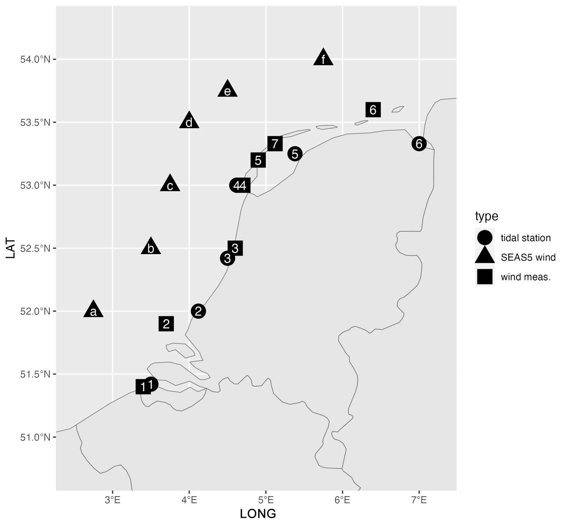
Figure 1 Locations of tidal stations (∘), SEAS5 output grid points (△) and weather stations (□). For numbering, refer to the main text.

High uncertainty has serious implications. Flood-protecting structures need to be over-designed, which is costly. Furthermore, over-designing requires that the uncertainty can be reliably quantified, but this is not the case for estimates from relatively short measurement records (see Sect. S1 in the Supplement). Hence, there is ample reason to look for ways to reduce the uncertainty in return values.

Besides coastal high water (HW, the peak water level reached during a high tide; see Appendix A), we will consider the wind shear stress (referred to as stress hereafter) in the atmospheric boundary layer over the coastal waters of the Netherlands. Stress generated by extratropical (ET) cyclones is the main driver of storm surge on the North Sea (e.g. Zweers et al., 2012). Hence, the reliability of estimates of return values of stress from simulation data is directly relevant to the reliability of return water level estimates from water level simulations forced by simulated stress data. Furthermore, stress also forces the sea surface waves which compound the impact of storm surge on the sea dikes, dunes and storm surge barriers (Van Nieuwkoop et al., 2015). Hence, it is the main link between atmospheric dynamics, surge and waves.

As stress is not routinely measured, it is often derived from wind speed measurements by an assumed drag relation, which is the subject of considerable disagreement and uncertainty (e.g. Van Nieuwkoop et al., 2015; Curcic, 2020; Richter et al., 2021). However, weather simulations provide data of stress near the surface. These data can be used to simulate nearshore wave spectra (e.g. Booij et al., 1999) and subsequently estimate return values of their height and period. Here, we focus instead on the stress itself to find out if return values of stress can be estimated reliably from simulated data. These return values can in fact be used together with tabulated nearshore wave model outputs to approximate return values for nearshore wave height and period (Groeneweg et al., 2010).

There is reason to be optimistic that simulated data for wind stress associated with ET cyclones may be useful for the estimation of return values. ET cyclones are relatively large-scale phenomena, and they are fairly well resolved by present-day global weather prediction models (Bauer et al., 2015). Starting from an atmosphere at rest, switching on the sun and rotating the earth at its known speed will soon result in realistic chaotic behaviour (Lorenz, 1969; Zhang et al., 2019): differential heating of the poles with respect to the Equator results in a temperature gradient driving the motions of air masses which (due to rotation) form jet streams, on which (due to barotropic and baroclinic instability) extratropical cyclones will develop. Even though these phenomena are complex and chaotic in appearance, they are governed by basic physics and are not particularly sensitive to poorly known or unresolved processes. For example, condensation and evaporation of water can have a considerable effect on the intensity of a particular storm, but the storms will be generated even without considering water in the atmosphere (Wernli and Gray, 2024).

On the other hand, biases in simulated large-scale forcing (e.g. the spatial distribution of solar irradiation), sea ice extent or varying large-scale circulation patterns may result in biases in the simulated jet stream strength and position as well as in storm frequency and intensity. In addition, errors in the representation of the aerodynamic drag of the sea surface (e.g. Makin et al., 1995) may cause biases in the simulated stress and hence in water levels simulated from that stress by a hydrodynamic model (e.g. Zweers et al., 2012).

In this article, we make the case that such biases do not necessarily preclude the use of simulated data for improving estimates of return values of stress and coastal HW. One reason is that an affine bias, i.e., a systematic error in the form of an added constant and/or multiplication by a positive constant, can be corrected effectively using relatively small datasets such as the measurement records of coastal water level spanning up to 140 years, as was confirmed in an earlier study (de Valk and van den Brink, 2023a). Stated differently: affine biases affect the location and scale parameters but not the shape. In contrast, estimation of the shape of the curve relating the frequency of exceedance μ(z) to the level z is notoriously difficult for high levels of z, and this is the main source of error in such estimates; see, for example, Chap. 4 of de Haan and Ferreira (2006) and de Valk and Cai (2018). This suggests that simulated data can and will be useful if these data make it possible to estimate the shape more accurately. Therefore, shape estimation is the main focus of our assessment.

In the next section, we describe the available datasets of measurements; reanalyses; and simulations of stress, near-surface wind, and water level. In Sect. 3, we introduce the concepts and methods from extreme value theory to be used for the estimation of frequencies of exceedance μ(z) (or return periods $T\left(z\right)=\mathrm{1}/\mathit{\mu }\left(z\right)$) of high levels of z and/or of the inverse relation expressing the return value as a function of its return period. In particular, we discuss different notions of shape in extreme value theory, as well as how they are connected.

In Sect. 4, we make the case that for stress over the North Sea, simulated data are suitable for shape estimation, and we argue in Sect. 5 that this extends to coastal water levels simulated from simulated stress and mean sea level pressure (mslp) fields. Furthermore, we propose a crude method for assessing the size of the residual unknown model-related bias in shape estimates and in estimates of return values, and we use this method to evaluate the reduction in uncertainty achieved by using simulated data for shape estimation (Sect. 6). Finally, we evaluate strengths and weaknesses of uncertainty reduction by shape estimation from simulated data, and we discuss the prospects for further improvements and generalization to other regions and/or variables (Sect. 7).

Note that labels for sections, figures, tables and equations containing “S” refer to the Supplement.

2 Data

SEAS5 stress and mslp. The primary source of simulated weather data for the present study is the archive of 6-hourly SEAS5 ensemble seasonal forecasts from the IFS cycle 43r1 model of ECMWF (ECMWF, 2018a, b) with nominal 35 km resolution. An ensemble of 25–50 seasonal forecasts over 7 months was started by ECMWF at the beginning of each month from 1981 onward. We use data of near-surface shear stress (vector), near-surface wind u₁₀ (vector) and mslp, discarding the first month of each run to ensure that the extremes of stress from different ensemble members are independent; for a verification, see Sect. S2. Stress and mslp are used to force tide-surge predictions (see below), and stress at the six points (shown by triangles in Fig. 1) is selected for statistical analysis. These points are at roughly 50 km from the shore to avoid any influence of land on surface roughness.

Stress and mslp from climate models and reanalyses. Data from climate model simulations used for checking of assumptions include a 16-member ensemble of EC-Earth3 runs for the present-day climate, as well as a dynamically downscaled version of these data produced using the RACMOv2.3 regional climate model (van Dorland et al., 2023). Furthermore, we use data from two reanalyses: ERA5, the most recent global reanalysis by ECMWF covering the years 1979–2019 (Hersbach et al., 2020), and KNW, a regional downscaling of ERA-Interim (Dee et al., 2011) (the predecessor of ERA5) for the North Sea over 1979–2019, produced by KNMI (Royal Netherlands Meteorological Institute) using the mesoscale model HARMONIE (Bengtsson et al., 2017). Validation of reanalysis wind against measurements is presented in Belmonte Rivas and Stoffelen (2019), Kalverla et al. (2019) and Wijnant et al. (2019) for ERA5 and in Stepek et al. (2015) and Wijnant et al. (2015, 2019) for KNW; see also further references in these articles. In particular, the empirical tail distributions of KNW wind speeds and of mast measurements are found to agree well (Stepek et al., 2015). These studies support the use of these two reanalyses for validation of statistics of stress from SEAS5.

Wind measurements. We use measurements of hourly mean wind from seven KNMI weather stations. Going along the coast from SW to NE, these are Cadzand (1), LEG (Lichteiland Goeree) (2), IJmuiden (3), Texelhors (4), Vlieland (5), West Terschelling (7) and Huibertgat (6), indicated by squares in Fig. 1.

Coastal tide gauge measurements. Time series of high water (HW) relative to the national NAP datum derived from measurements are available from Rijkswaterstaat. Here, we consider (from SW to NE) data from Vlissingen (1), Hoek van Holland (2), IJmuiden (3), Den Helder (4), Harlingen (5) and Delfzijl (6), indicated by circles in Fig. 1. Records begin around 1880–1890 (1, 2, 3, 6) or around 1932 (4, 5). Long-term trends were estimated by fitting smooth curves to the records of annual mean HW, and they are subsequently removed; see Sect. S3. The homogenized values are representative for the year 2019.

Coastal water levels simulated from SEAS5 data. Still water levels on the North Sea were simulated using the WAQUA DCSMv5 shelf-sea tide and surge prediction model with 8 km resolution (Ridder et al., 2018), forced by SEAS5 stress and mslp; see van den Brink (2020). This resulted in 10 min time series for over 300 locations along the Dutch coast, including the six tidal stations listed above. From these, records of high water (HW) were derived using the astronomical tide computed by running DCSMv5 without variation in meteorological forcing. We refer to these data as SEAS5/DCSMv5 data. Furthermore, the same simulation was performed with the stress forcing increased by 10 %.

Additional water level simulations were performed for 250 storms selected from the SEAS5 archive, downscaled using the regional mesoscale HARMONIE model (Bengtsson et al., 2017); see van den Brink (2020) for details. These simulations were performed with two models: DCSMv5 (see above) and DCSM-FM 100 m, which has a much higher resolution.

3 Methods

3.1 Background: return values and tail approximation

For statistical analysis, extreme weather events like storms are generally regarded as clusters of high values occurring at random times, approximated by a Poisson process (e.g. Leadbetter, 1982; Leadbetter et al., 1983) with seasonally varying intensity. This implies that the distribution of the maximum of a variable X over T entire years can be represented as

$$\begin{array}{}\text{(1)}& \mathbb{P}\left(\underset{t\in [\mathrm{0},T]}{max}{X}_t\le z\right)=e^{-\mathit{\mu }\left(z\right)T},\end{array}$$

with μ(z) being the frequency of exceedance (in clusters per year) of the level z, given by

$$\begin{array}{}\text{(2)}& \mathit{\mu }\left(z\right)=(\mathrm{1}-F(z\left)\right)\mathit{\alpha }/\mathrm{\Delta },\end{array}$$

where F is the average distribution function of X over the year; Δ is the time step of the data record; and α is the extremal index, which may be regarded as the reciprocal of the mean cluster length in time steps (so $\mathrm{\Delta }/\mathit{\alpha }$ is the mean cluster length in years).

To estimate low probabilities of exceedance 1−F(z) of high levels of z, one needs to assume a certain regularity of the upper tail of F, which allows for extrapolation of F from a high level of z to (much) higher levels. Non-regularity may occur, for example, in mixtures of distributions of subpopulations with different tails (e.g. frontal vs. convective sub-daily rainfall intensity) or due to a change in the physics of a process near some threshold (e.g. the limitation of sea surface wave growth by breaking on shallow water). We discuss two alternative regularity assumptions here in the context of smooth tails. These assumptions are conveniently expressed in terms of the “quantile function” q defined by

$$\begin{array}{}\text{(3)}& \mathrm{1}-F\left(q\right(y\left)\right)=e^{-y},y\ge \mathrm{0};\end{array}$$

q expresses any quantile of the distribution F in terms of the quantile of the exponential distribution for the same probability. Using Eq. (2), the return value R_T for a return period T can be written as

$$\begin{array}{}\text{(4)}& R_T=q\left(\log \right(T\mathit{\alpha }/\mathrm{\Delta }\left)\right).\end{array}$$

We define the function $\stackrel{\mathrm{̃}}{\mathit{\gamma }}$ by

$$\begin{array}{}\text{(5)}& \stackrel{\mathrm{̃}}{\mathit{\gamma }}\left(y\right):=q^{\prime \prime }\left(y\right)/q^{\prime }\left(y\right)=\left(\log q^{\prime }\right(y){)}^{\prime },\end{array}$$

with ^′ indicating the derivative. $\stackrel{\mathrm{̃}}{\mathit{\gamma }}$ can be regarded as a dimensionless curvature of the quantile function q. The most familiar regularity assumption is

$$\begin{array}{}\text{(6)}& \underset{y\to \mathrm{\infty }}{lim}\stackrel{\mathrm{̃}}{\mathit{\gamma }}\left(y\right)=\underset{y\to \mathrm{\infty }}{lim}\left(\log q^{\prime }\right(y){)}^{\prime }=\mathit{\gamma }\end{array}$$

for some real number γ (e.g. de Haan and Ferreira, 2006, Corollary 1.1.10). By integration, this implies

$$\begin{array}{}\text{(7)}& \underset{y\to \mathrm{\infty }}{lim}{\displaystyle \frac{q(y+x)-q\left(y\right)}{q^{\prime }\left(y\right)}}={\displaystyle \frac{e^{x\mathit{\gamma }}-\mathrm{1}}{\mathit{\gamma }}},x\in \mathbb{R}\end{array}$$

(to be read as x if γ=0). Equation (7) provides a recipe for approximating a higher quantile q(y+x) exceeded with probability $e^{-(y+x)}$ from a lower quantile q(y) exceeded with probability e^−y. It is one of the formulations of the generalized Pareto (GP) tail limit employed in classical peak-over-threshold analysis (Leadbetter, 1991; Coles, 2001; de Haan and Ferreira, 2006). The number γ is the GP tail shape parameter; by Eq. (6), we can regard the function $\stackrel{\mathrm{̃}}{\mathit{\gamma }}$ as a pre-asymptotic GP shape.

The GP tail limit (Eq. 7) is equivalent to the assumption that the distribution of the appropriately scaled and shifted maximum of a random sample $X_{\mathrm{1}},\mathrm{\dots },X_n$ tends to a non-constant limit as n→∞ (de Haan and Ferreira, 2006), known as a GEV (generalized extreme value) distribution. It has the same shape parameter γ as the GP tail limit. Furthermore, clustering of high values only affects the scale and location parameters of the GEV (Leadbetter, 1982; Leadbetter et al., 1983).

There is ample evidence that the assumption γ=0 is appropriate for the square of wind speed (e.g. Cook, 1982; Harris, 2005; van den Brink and Können, 2008). By extension, the same must hold for stress and surge level: these quantities are nearly proportional to the square of wind speed; therefore, their tails must also have γ≈0.

Another regularity assumption, particularly useful as a refinement of Eq. (6) if γ=0, replaces the derivatives to y in Eq. (6) by derivatives to log y:

$$\begin{array}{}\text{(8)}& \underset{y\to \mathrm{\infty }}{lim}y{\left(\log \left(y{q}^{\prime }\right(y\left)\right)\right)}^{\prime }=\underset{y\to \mathrm{\infty }}{lim}y\stackrel{\mathrm{̃}}{\mathit{\gamma }}\left(y\right)+\mathrm{1}=\mathit{\beta }\in \mathbb{R}.\end{array}$$

This leads to the generalized Weibull (GW) limit (de Valk, 2016):

$$\begin{array}{}\text{(9)}& \underset{y\to \mathrm{\infty }}{lim}{\displaystyle \frac{q\left(y\mathit{\lambda }\right)-q\left(y\right)}{y{q}^{\prime }\left(y\right)}}={\displaystyle \frac{{\mathit{\lambda }}^{\mathit{\beta }}-\mathrm{1}}{\mathit{\beta }}},\mathit{\lambda }>\mathrm{0},\end{array}$$

providing an alternative recipe for estimating high quantiles. In the case of β>0, tail approximations based on Eq. (9) take the form of a three-parameter (translated) Weibull distribution: $\log P(X>x)=-\left(\right(x-b)/a{)}^{\mathrm{1}/\mathit{\beta }}$ for some b∈ℝ and a>0. This helps with interpreting the GW tail shape parameter β (e.g. β=1 gives a shifted exponential tail, β=0.5 a shifted Rayleigh tail). Unlike Eq. (7), Eq. (9) approximates q over a probability range which increases rapidly with y. For estimating return values with very large return periods, this makes the GW tail preferable over the GP tail if both tail limits hold.

The simple relation between the pre-asymptotic GP shape $\stackrel{\mathrm{̃}}{\mathit{\gamma }}\left(y\right)$ and the pre-asymptotic GW shape $y\stackrel{\mathrm{̃}}{\mathit{\gamma }}\left(y\right)+\mathrm{1}$ shows that for comparing shapes (e.g. of tails of data from different sources), we can use either.

3.2 Estimation

Estimates of tails and tail statistics like the extremal index are derived from the values in the data record above a chosen threshold. We choose and report the fraction p of the sample above the threshold, which is more informative than the threshold itself.

Given the sample fraction p and corresponding $y=\log (\mathrm{1}/p)$, the location parameter q(y) of the GP and GW tails (Eqs. 7 and 9) are estimated by the ⌈pn⌉th largest value in the sample, with ⌈⋅⌉ indicating rounding upwards. The scale parameter q^′(y) and shape parameter γ of the GP tail (Eq. 7) are estimated from the ⌈pn⌉th largest values by the maximum likelihood estimator (de Haan and Ferreira, 2006). For the GW tail Eq. (9), the scale parameter yq^′(y) and shape parameter β are estimated from the ⌈pn⌉th largest values by an adaptation of the method of de Valk and Cai (2018); see Sect. S6 for details. These estimators can be applied with fixed values of the shape parameter; this makes it easy to combine the shape estimate from one dataset with scale and location estimation from another dataset.

When combining scale and location estimation from one dataset with a shape estimate from another dataset, the same method and the same sample fraction p are used.

Plots of the GW shape estimates against the sample fraction p (the latter on a logarithmic scale) provide information about the pre-asymptotic shape $y\stackrel{\mathrm{̃}}{\mathit{\gamma }}\left(y\right)+\mathrm{1}$ at y near $\log (\mathrm{1}/p)$ (see Eq. 8). In fact, the estimator has been constructed to estimate this pre-asymptotic shape (see de Valk and Cai, 2018). Such a plot is usually made to check a regularity assumption (in this case, convergence of $y\stackrel{\mathrm{̃}}{\mathit{\gamma }}\left(y\right)+\mathrm{1}$ to a limiting value β). However, whether or not regularity assumptions apply, it is very useful for comparing the shapes of tails of data from different sources. For this purpose, the pre-asymptotic GW tail shape $y\stackrel{\mathrm{̃}}{\mathit{\gamma }}\left(y\right)+\mathrm{1}$ is more informative than the pre-asymptotic GP shape γ(y): with increasing y (decreasing sample fraction p), shape variations are magnified.

For the comparison of shape estimates from very large datasets of thousands of years of model-generated weather data at many grid points, these methods are not practical, as the data from all time steps are required for the estimates. Instead, we fit for each grid point a GEV distribution to the annual maxima by the maximum likelihood method (e.g. Dombry, 2015), which provides an estimate of $\stackrel{\mathrm{̃}}{\mathit{\gamma }}\left(y\right)$ at $y\approx \log (\mathit{\alpha }/\mathrm{\Delta })$ corresponding to a 1 yr⁻¹ event. In practice, this tends to result in somewhat higher estimates of γ than a GP tail estimate from all data above a threshold, but that is no problem for comparing estimates from different datasets.

The extremal index α (see Eq. 2) is chosen based on estimates of α from data for the months December, January and February (DJF) only, in order to minimize bias due to seasonality. We apply the method of Ferro and Segers (2003) using various thresholds in order to check the dependence on the fraction p of the sample above the threshold.

3.3 Estimation error

Different methods are used to estimate the sampling error (Appendix A) of estimates of return values and tail parameters.

For GW and GP tail parameter and return value estimates, a bootstrap method (e.g. Litvinova and Silvapulle, 2018, 2020; de Haan and Zhou, 2022) is used. More specifically, we use the block bootstrap (Künsch, 1989) to estimate variances, which is applicable to serially dependent time series. In the block bootstrap, the analysed time series are divided into blocks longer than the typical decorrelation time, and new synthetic time series of the same length as the original series are constructed by randomly drawing blocks with replacement and placing one after the other. The entire data analysis is performed on 100 synthetic time series, and the variance of the statistic of interest is estimated by the empirical variance of its values calculated from these series.

For the measurement data, blocks of 1 year are used to preserve the seasonality in the data. For SEAS5 seasonal forecasts of stress and for HW simulated from SEAS5 data (see Sect. 2), blocks consisting of 6-month-long forecast runs were used. In principle, the selection of 6-month blocks introduces a spurious inflation of the variance due to the seasonality (e.g., there may be too many or too few winter months in the resampled dataset), but this effect was shown to be negligible, due to the large size of the dataset.

For estimates derived from seasonal forecasts, this bootstrap method requires independence of the members of a forecast ensemble. For stress, this has been verified; see Sect. S2.

For estimates of γ from GEV fits to annual maxima (see Sect. 3.2), independence of annual maxima is assumed, and the asymptotic approximation of the variance is used (e.g. Dombry, 2015).

Confidence intervals are derived from estimated variances using the normal approximation.

4 Can we trust the tail shape of stress over the North Sea derived from simulated data?

4.1 Overview

In this section, we argue that (a) large-scale metrics of storm intensity such as mslp have regular tails; (b) climate models of sufficient resolution show high skill at simulating extratropical cyclones and agree about the tail shapes of mslp distributions; (c) stress in the boundary layer is closely linked with overall storm intensity; and (d) the tail of the stress distribution is also regular, and its shape can be estimated reliably from climate model simulations. We will use the term climate model for any model run for a considerable time without data assimilation, which includes the selected SEAS data used in this study (Sect. 2).

4.2 Large-scale metrics of storm intensity are expected to have regular tails

Coastal flood risk in the Netherlands is determined by extratropical cyclones in the winter storm season. Extratropical cyclones are a well-defined phenomenon; variations in their development constitute a continuum (Graf et al., 2017; Seiler, 2019). Therefore, tail anomalies due to mixing subpopulations with distinctly different tails are not an issue. Furthermore, the growth of extratropical cyclones does not appear to involve sharp transitions or limits at a certain intensity level which could give rise to a tail anomaly.

Common metrics of overall storm intensity are, for example, the spatio-temporal minimum of mslp or maximum of relative vorticity at 850 hPa. Because the density of storm tracks varies smoothly, we may expect that the values at a fixed location also have smooth tails. This is illustrated by Fig. 2 in Sterl et al. (2009) or Fig. 2 here, showing the empirical return values of daily-averaged mslp from 147 years of measurements at Thyboron (8.2° E, 56.7° N) on the west coast of Denmark, from the RACMOv2.3 and EC-Earth3bis climate model simulations (see Sect. 2), as well as from SEAS5. A low mslp at this site indicates the presence of a low-pressure area nearby, resulting in a north-westerly wind over the North Sea and a positive surge at the Dutch coast. The modelled tails are indeed smooth (very long series); the measurement record is much shorter; hence, the empirical distribution of the annual minima is more noisy but agrees reasonably well with the modelled tails.

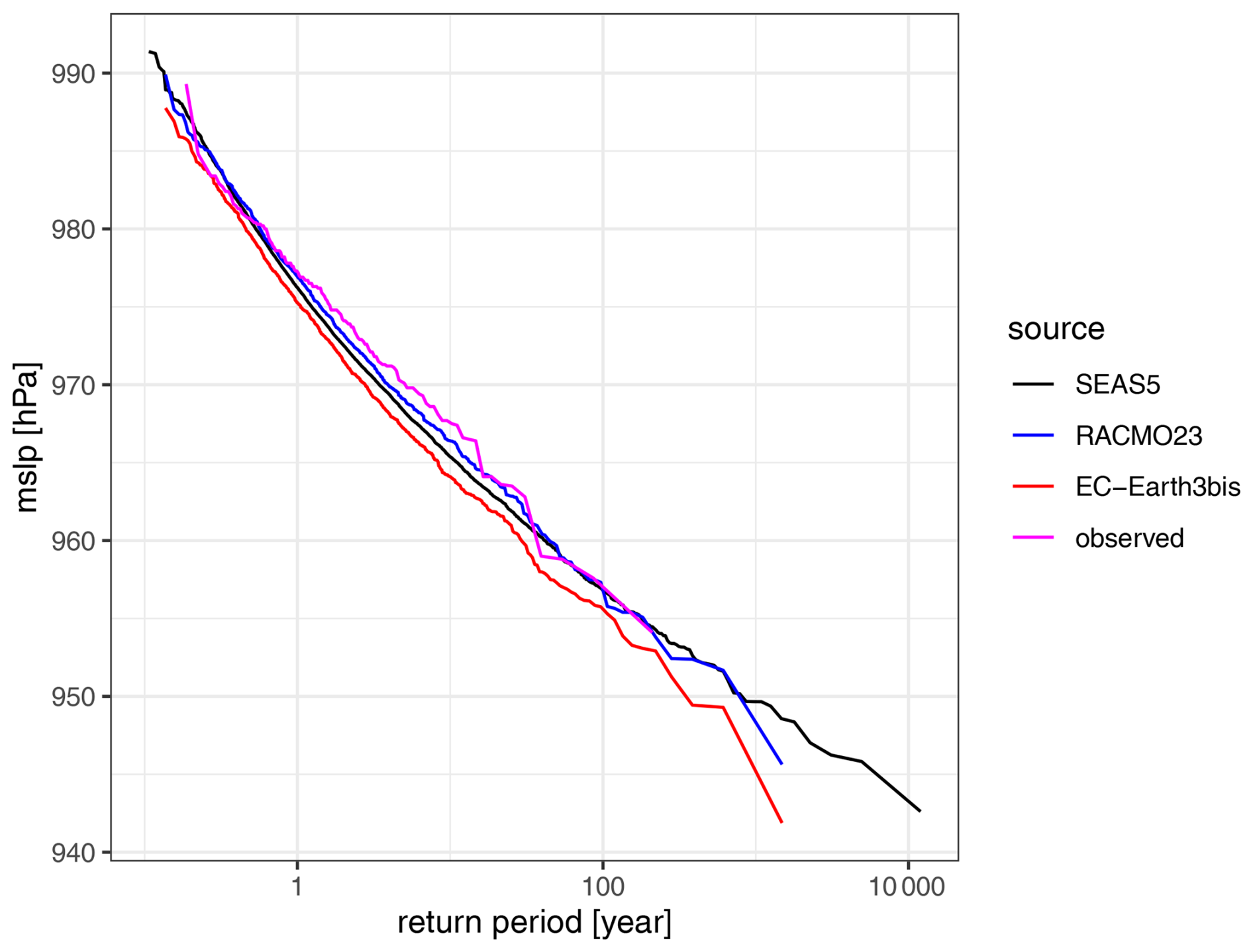
Figure 2 Empirical return values from annual maxima of daily-mean mslp near 8.2° E, 56.7° N from SEAS5 (black), RACMOv2.3 (blue) and EC-Earth3bis (red) as well as from measurements at Thyboron (Denmark) over 1874–2020 (magenta).

4.3 Climate models of sufficient resolution show high skill at simulating extratropical cyclones and agree about the tail shapes of mslp distributions

More than a decade ago, climate models already produced skilful simulations of extratropical cyclones when comparing the intensity, tracks and storm structure to reanalysis data (Catto et al., 2010; Bengtsson et al., 2009; Jung et al., 2012). Then and now, a sufficiently high resolution (25–50 km) is a requirement (Priestley and Catto, 2022), but a further increase in resolution offers limited benefit (Jung et al., 2012). Remaining limitations appear to mainly concern the flow in the upper atmosphere (250 hPa). The resolution of SEAS5 of about of 0.25° should thus be sufficient for the simulation of coastal surges and waves requiring a long fetch and duration to develop. Indeed, van den Brink (2020) shows that the limited resolution of SEAS5 only gives a 1.5 % reduction in surge and a further 3.5 % reduction due to 6-hourly sampling of the SEAS5 output, in comparison with the hourly sampled 2.5 km resolution HARMONIE model output (Sect. 2).

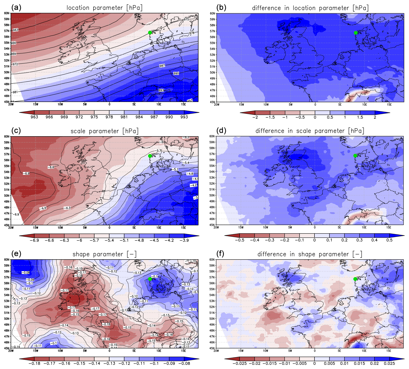
Figure 3 Spatial patterns of estimates of location, scale and shape (γ) (see Sect. 3.1) of the GEV distribution fitted to the annual minimum mslp. (a, c, e) From RACMOv2.3 (colours) and from EC-Earth3bis (contours). (b, d, f) Differences (RACMOv2.3 minus EC-Earth3bis); the green dot indicates Thyboron.

The high skill is particularly evident in the tail shapes of storm intensity metrics. In Fig. 2, the shapes and scales of distributions of annual minima of daily-mean mslp from RACMOv2.3, EC-Earth3bis and SEAS5 show remarkable agreement: the main differences are small (but significant) shifts in pressure and even smaller differences in scale. All agree closely with the empirical tail from the observations and are capable of generating deeper depressions than observed at this location. Figure 3 displays estimates of the GEV parameters from the annual maxima of daily-averaged mslp over the North Sea from effectively 1040 years of EC-Earth3bis and its downscaling with the regional RACMOv2.3, as well as their difference. It shows excellent spatial agreement between these models. The standard error of the estimates of the shape parameter γ is about 0.02, implying that the cluttered difference in shape is insignificant at all grid points. This confirms that the considerable differences in resolution and boundary layer parameterization of these models leave the shape of the mslp tail virtually unaffected. This is remarkable, as these simulated storms and their climatologies are generated completely by the models, unlike numerical weather forecasts.

4.4 Stress in the boundary layer is closely linked with overall storm intensity

Stress in the boundary layer over sea depends on the wind aloft, stability, and the interaction with the sea surface, which are all different in different sectors of the storm. In turn, the stress affects the evolution of the storm by barotropic (e.g. Ekman pumping) and baroclinic potential vorticity generation in the boundary layer. In a modelling study of dry extratropical cyclone formation, Beare (2007) found that the spatial maximum of surface stress at every instant scales in a simple way with the initial strength of the jet stream. Furthermore, if the boundary layer parameterization is changed, changes in the minimum pressure correspond closely to changes in the surface stress averaged over the cyclone. Beare (2007) concludes that this demonstrates the important role of the synoptic-scale flow in organizing the boundary layer structure. Boutle et al. (2015) complete this picture by detailing how barotropic and baroclinic potential vorticity generation act together to reduce cyclone growth. Furthermore, Boutle et al. (2010) discuss the roles of moisture transport and convection; they show that the spin-down due to surface friction is of similar magnitude in a moist cyclone as in a dry cyclone.

4.5 The tail of the stress distribution is also regular, and its shape can be estimated reliably from climate model simulations

Section 4.2 and 4.4 imply that the tail of the distribution function of stress is also highly regular; possible saturation of the drag coefficient over sea at high wind speeds (Curcic, 2020; Richter et al., 2021) is not likely to change this; see Sect. S4. Climate model simulations indicate that this is indeed so: Fig. 4 shows the distributions of annual maxima of stress from 3-hourly RACMOv2.3 and 6-hourly SEAS5 data. These two tails clearly differ in scale (likely as a result of differences in boundary layer parameterization, as the scale is lower for stress from the high-resolution RACMOv2.3 model). However, the shapes agree closely; both are nearly exponential.

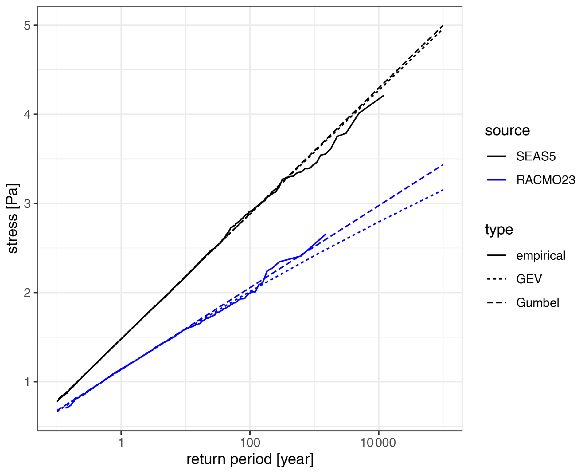
Figure 4 Empirical return values of stress from annual maxima at 3.5° E, 54° N from 3-hourly RACMOv2.3 (blue) and 6-hourly SEAS5 (black) data, with return values from GEV fits (dotted) and from Gumbel fits (dashed).

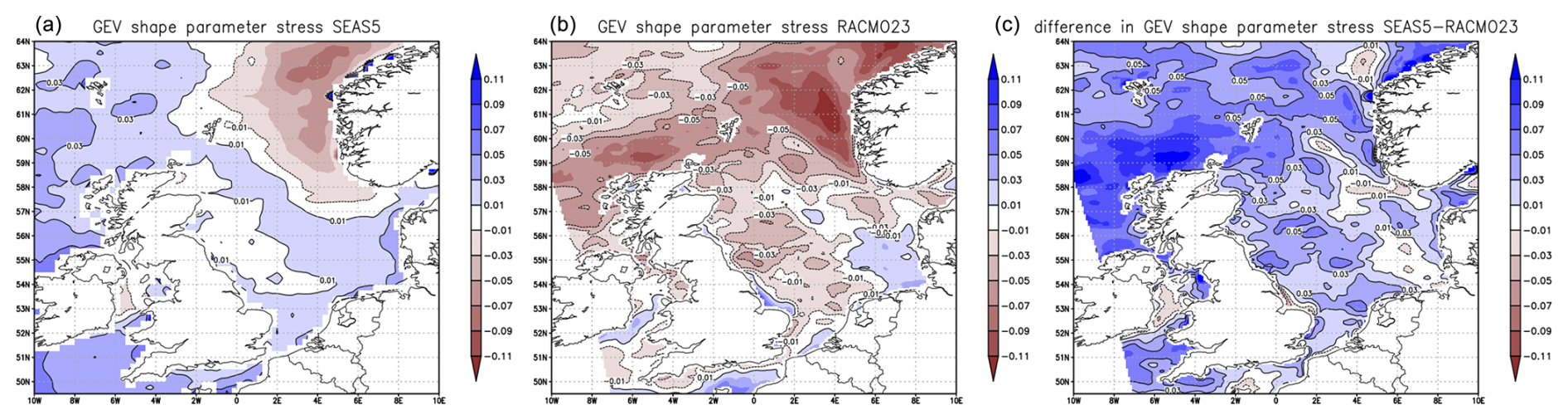
Figure 5 Estimates of the tail shape γ (see Sect. 3.1) from annual stress maxima from SEAS5 (a) and from RACMOv2.3 downscaling of EC-Earth3bis runs (b), as well as their differences (c).

Both models have different resolutions and output frequencies, and the boundary layer parameterizations are quite different, but this appears to have little impact on the shape of the stress tail. This is also evident from Fig. 5, showing estimates of the GEV shape γ from annual stress maxima over the North Sea. On average, the estimates from SEAS5 are slightly lower than the estimates from RACMOv2.3, differing on average over the central and southern North Sea by 0.026, which is not much. The close agreement in the tail shape of stress from these models indicates that the shape is determined by other factors than resolution, output frequency or boundary layer parameterization, such as jet stream climatology (Sect. 4.4).

Another relevant check is to compare estimates of the shape of the tail of stress from SEAS5 with those from the reanalyses ERA5 and KNW for the same position of 3° E, 55° N in the central North Sea, far from the influence of land; see Sect. 2. Plotted as functions of sample fraction $p=k/n$, estimates of the GW shape parameter β (see Eqs. 8, 9) can be regarded as estimates of the dimensionless shape function $y\left(\log \right(y{q}^{\prime }\left(y\right)){)}^{\prime }$, with $y=-\log p$. Figure 6 shows for SEAS5 only a slight increase in these estimates with decreasing p from about 1.2 to 1.35, which indicates a regular tail which is slightly heavier than the exponential tail. Furthermore, the estimates match the much-less-precise estimates from the two reanalysis datasets which, unlike the SEAS5 forecasts (with lead times exceeding 1 month), are constrained by weather observations and employ significantly different resolutions and different approaches to boundary layer momentum exchange. This provides further confirmation that current climate models are capable of simulating the shape of the stress tail.

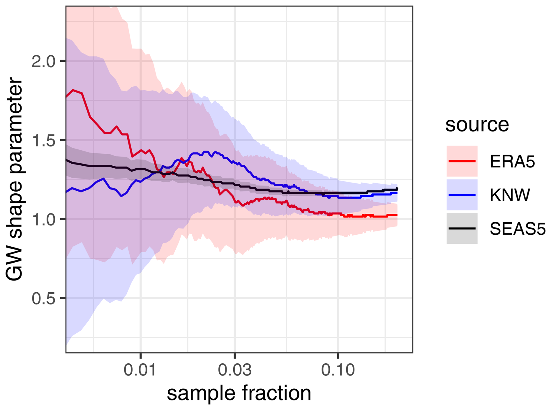
Figure 6 Estimates of the GW shape parameter β (see Sect. 3.1) of stress from SEAS5 with 95 % confidence intervals (black) and from the KNW reanalysis (blue) and the ERA5 reanalysis (red), along with their confidence intervals at 3° E, 55° N (central North Sea). The horizontal axis indicates the sample fraction $k/n$ used for the estimation (see text).

As a consequence, systematic errors in extreme stress from these models should take the form of scale/location errors. This agrees broadly with the analysis in Larsén (2012) of the effect of limited resolution on extreme wind speeds over Danish and German coastal waters from mesoscale models; for a Gaussian process as approximation of wind fluctuations, they argue that the correction should have the form of a scale adjustment. Although Larsén (2012) do not consider the effects of differences in boundary layer parameterization of the mesoscale models used for downscaling of global low-resolution analyses, their corrected estimates of mean annual maximum wind speed from these models are mutually compatible and in line with wind measurements. In climate model simulations and in SEAS5 (for forecast ranges exceeding 1 month), storms are generated by the model without assimilation of measurements, which offers much additional freedom to deviate from observed climatology. Our findings indicate that even in this case the shape of the stress tail generated by such models is reliable over a wide range of return periods.

5 How reliable are the shapes of the tails of HW along the Dutch coast derived from simulated data?

Since stress provides the main forcing of a storm surge, it can be expected that the tails of the surge and HW along the Dutch coast are also regular. They should in fact be similar to the tail of stress, as storm surge is roughly proportional to the stress if we ignore the effects of wind directionality, fetch and duration limitations, and along-shore flow. Whether their shapes can be reliably estimated from hydrodynamic model simulations forced by model-generated stress depends on the size and nature of the bias in these models.

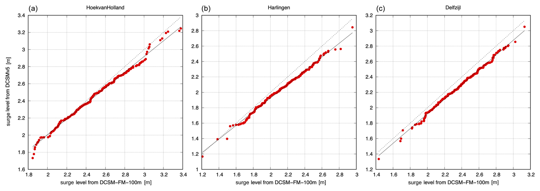
Figure 7 Sorted peak values of skew surge [m] of 250 storms from DSCMv5 versus DCSM-FM-100 m (Q-Q plot) for Hoek van Holland (a), Harlingen (b) and Delfzijl (c) with fitted affine relation (full line).

Systematic differences between skew surge from different models appear to be affine (“linear plus constant”; see Appendix A). As an example, Fig. 7 shows for two sites the relationship between skew surge predictions from the low-resolution DCSMv5 model and the high-resolution DCSM-FM 100 m model. These were determined from water level simulations for 250 downscaled severe storms from the SEAS5 archive (Sect. 2). Affine relations are also found at all other sites (not shown). This indicates that the resolution of the surge-tide model does not affect the shape parameter of the tail of skew surge (and therefore does not affect the shape of the HW tail either).

Validation of the DCSM-FM 100 m model against measurements in Zijl et al. (2022) and Zijl and Laan (2021) shows that predicted skew surge at tidal stations on the Wadden Sea (with labels 4–6 in Fig. 1) has a negative bias for surge above a threshold close to the 99 % quantile; the magnitude of this bias increases approximately linearly in the excess of surge above this threshold; see Fig. S7 (Sect. S7). A similar bias pattern was already reported in Ridder et al. (2018) for the DCSMv5 model. This suggests either an issue with the representation of hydrodynamic processes in the shallow Wadden Sea estuary under severe storm conditions (e.g. wave–current interaction or changes of the seabed and its roughness) or insufficient resolution of mesoscale variations of stress, which would affect the shallow Wadden Sea more than the adjacent North Sea. Modelling experiments with varying forcing and resolution seem to point to the former explanation (van den Brink, 2020), but the issue has not been resolved yet.

Figure 8 Estimates of the GW shape parameter β (see Sect. 3.1) of HW vs. sample fraction with 95 % confidence interval from measurements (blue) and from SEAS5/DCSMv5 simulations (black) for 6 tide gauge stations (see Fig. 1).

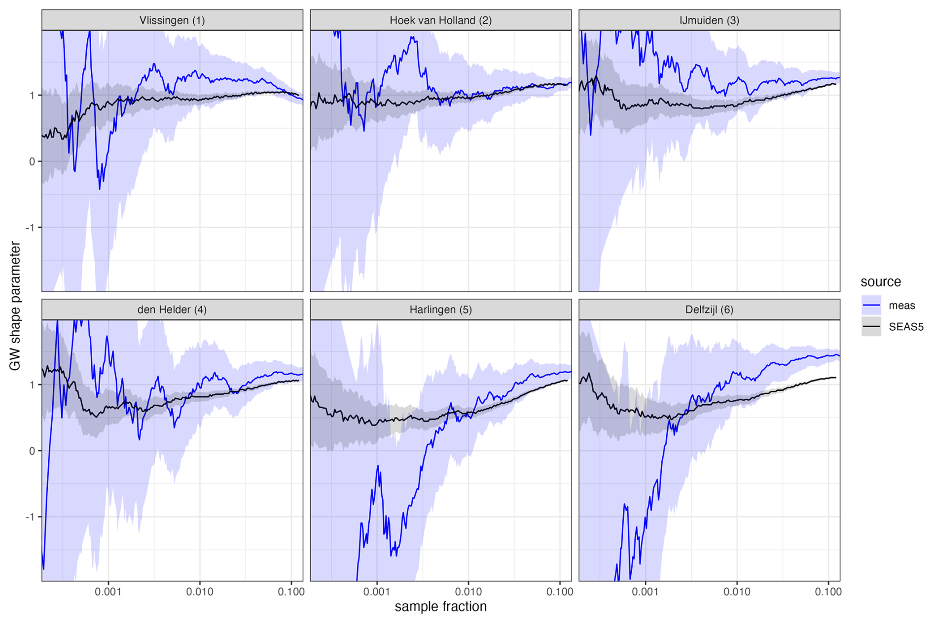
The apparently linear bias in the excess of skew surge (Appendix A) above a threshold suggests that the shapes of surge and HW tails estimated from the model simulations may still be accurate above this threshold. To check this, GW tail shape estimates from tide gauge data and simulations are compared in Fig. 8. Indeed, the estimates from the SEAS5/DCSMv5 data are compatible with the estimates from tide gauge data for five of the six tide gauge stations. The exception is Delfzijl (6) on the small Eems-Dollard estuary (Fig. 1). The poor match at high sample fractions above say 0.01 for Delfzijl may be related to the change in bias in model predictions of skew surge from negligible to negative at roughly the 99 % quantile found in Zijl and Laan (2021) (see Fig. S7 in Sect. S7), which will distort shape estimates at mentioned sample fractions. This is confirmed by Fig. S8 (Sect. S7), showing the effect of such a bias on shape estimates.

Note that the shape estimates from the measurements at Harlingen (5) and Delfzijl (6) are highly irregular at sample fractions below 0.005, which is not plausible in view of the regularity of the estimates at other stations nearby and the considerable spatial coherence in storm surge on the North Sea. The wide confidence intervals of these estimates indicate that they are not reliable. This suggests that the use of SEAS5/DCSMv5 data for shape estimation has the additional benefit of ensuring that spatial variations in tail shape are plausible.

6 Estimation of return values of stress and coastal water level using simulated data and measurements

6.1 Introduction

The previous sections presented evidence in support of estimation of the shapes of the tails of stress and HW from simulated data. Here, we discuss how this can be put into practice and assess the uncertainty of the resulting estimates, which includes the sampling error (see Appendix A) and the unknown residual model-related bias in estimates from simulated data.

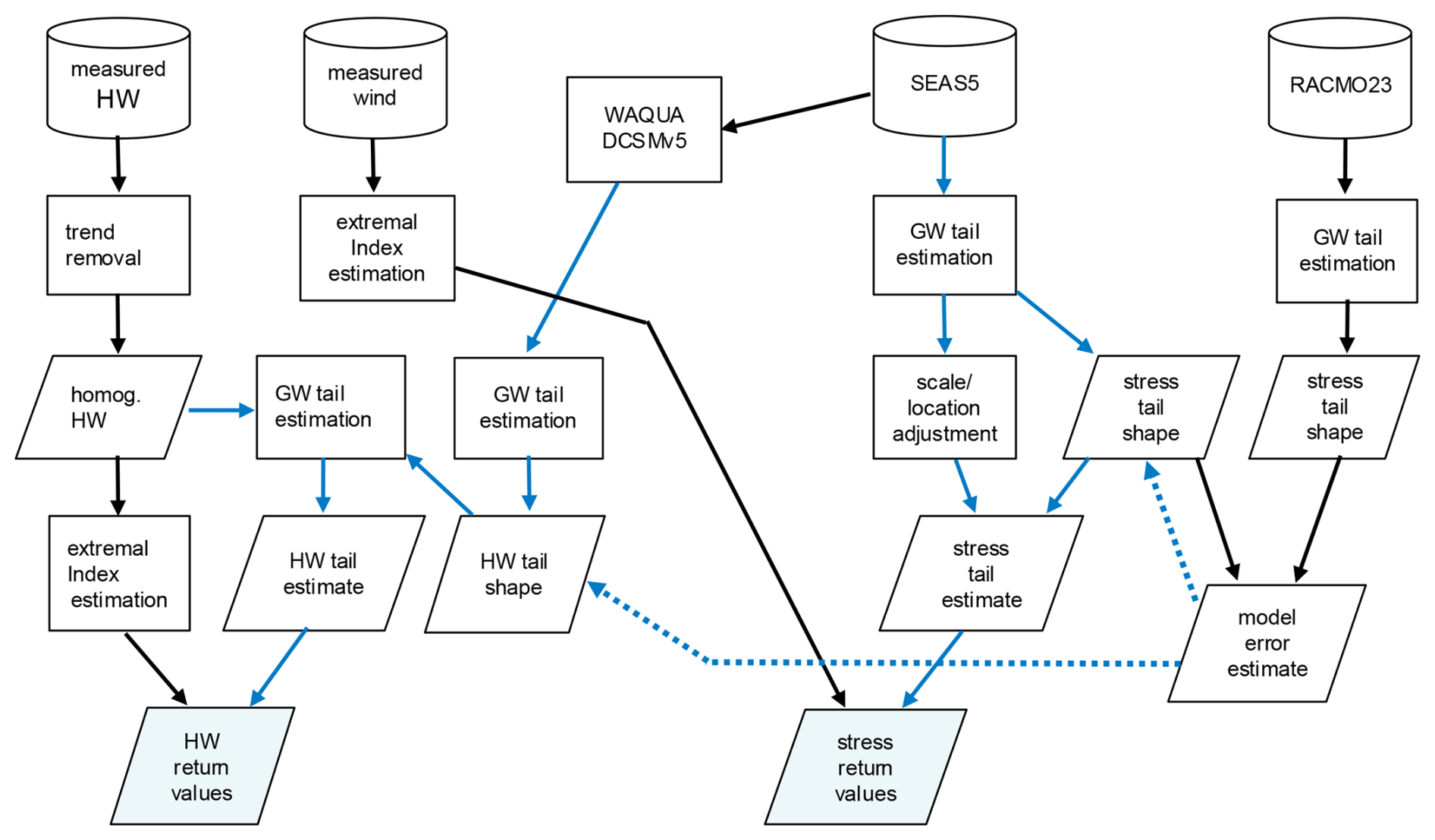
Figure 9 Overview of the proposed method for estimating return values of stress and coastal high water (HW). Cylinder: archive (see Sect. 2). Rectangle: processing. Parallelogram: data. Blue arrow: data flow with propagation of uncertainty. Dotted blue arrow: propagation of uncertainty only.

The procedures applied for stress and for HW are somewhat different, as we have water level measurements but no measurements of stress. A diagram summarizing the data and processing steps is shown in Fig. 9.

For tail estimation, we use the GW tail approximation Eq. (9). This choice is based on the results of an earlier study (de Valk and van den Brink, 2023a), employing Monte Carlo simulation based on estimates of distribution functions for wind speed, skew surge and HW from the long archive of SEAS5/DCSMv5 data (Sect. 2) using a refined method, which allows for the estimation of deviations from limiting GP and GW tail shapes. This study found that if the tail shape of HW is estimated from a record similar in size to a measurement record, the GW tail produces considerably more accurate estimates than the GP tail. However, this difference largely disappears if a record of the size of the local SEAS5 data is used for shape estimation. For wind speed, the GW tail was found to perform considerably better than the GP tail, also when very long records are used for shape estimation (de Valk and van den Brink, 2023a, Appendix C).

For the estimation (see Sect. 3.2), thresholds exceeded by a sample fraction p=0.012 are used, based on the same simulation study. This choice is verified using threshold plots like Figs. 6 and 8.

Return values are estimated using Eq. (2) with values of the extremal index α to be discussed below.

6.2 Stress

GW tails of stress are estimated from 6-hourly SEAS5 stress data at the grid points marked by triangles in Fig. 1. Note that 1−F in Eq. (2) represents a fraction of time, which has the same meaning regardless of sampling interval. Therefore, the sparse temporal sampling of the SEAS5 data is not expected to affect the estimation of F or its quantile function q. However, it is a problem for estimation of the extremal index α.

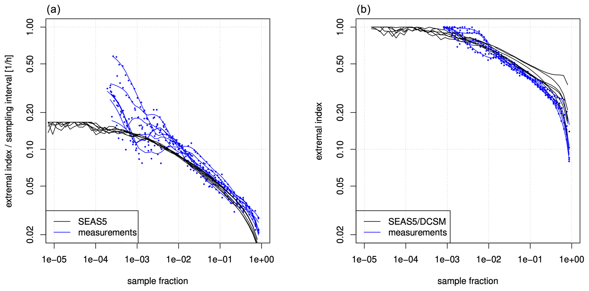
Figure 10 (a) Estimates of the extremal index divided by time step for SEAS5 stress (black lines) and measured wind speed (blue dots) in the months DJF. (b) Estimates of the extremal index for HW in DJF from SEAS5/DCSMv5 data (black lines) and measurements (blue dots). Blue lines are smoothed estimates from measurements. Each line corresponds to a grid point or station.

Figure 10 (left) shows estimates of the ratio of α to the sampling interval derived from SEAS5 stress and from hourly measurements of wind speed u₁₀ at all sites (see Fig. 1); this ratio is the quantity that matters for the computation of return values by Eq. (4). The extremal indices for stress and for wind speed u₁₀ should be the same, since the extremal index is not affected by a monotonic transformation. The estimates from the SEAS5 data tend to the maximum possible value of $\mathrm{1}/\mathrm{6}$ h⁻¹ with decreasing sample fraction, but the estimates from the wind speed measurements keep increasing. Such a continued increase is typical for a Gaussian process (e.g. Leadbetter et al., 1983), which has been used as a model for wind speed fluctuations before (Larsén, 2012). In this case, all one can do is choose a value which is consistent with the estimates and is suitable for the application. Since for flood risk assessment (a) wind stress is only used to determine hydraulic loads on the coastal structure and since (b) these tend to vary more slowly than the hourly wind speed or wind stress, we somewhat arbitrarily adopt 0.5 h⁻¹, corresponding to a mean cluster length of 2 h. This choice is close to the highest estimates in Fig. 10 (left).

Finally, the scale and location parameters are increased by a factor of 1.1 (giving a uniform increase of all return values by the same factor), based on an earlier analysis of the effects of atmospheric model resolution on skew surge in van den Brink (2020). We refer to the diagram of Fig. 9 for an overview.

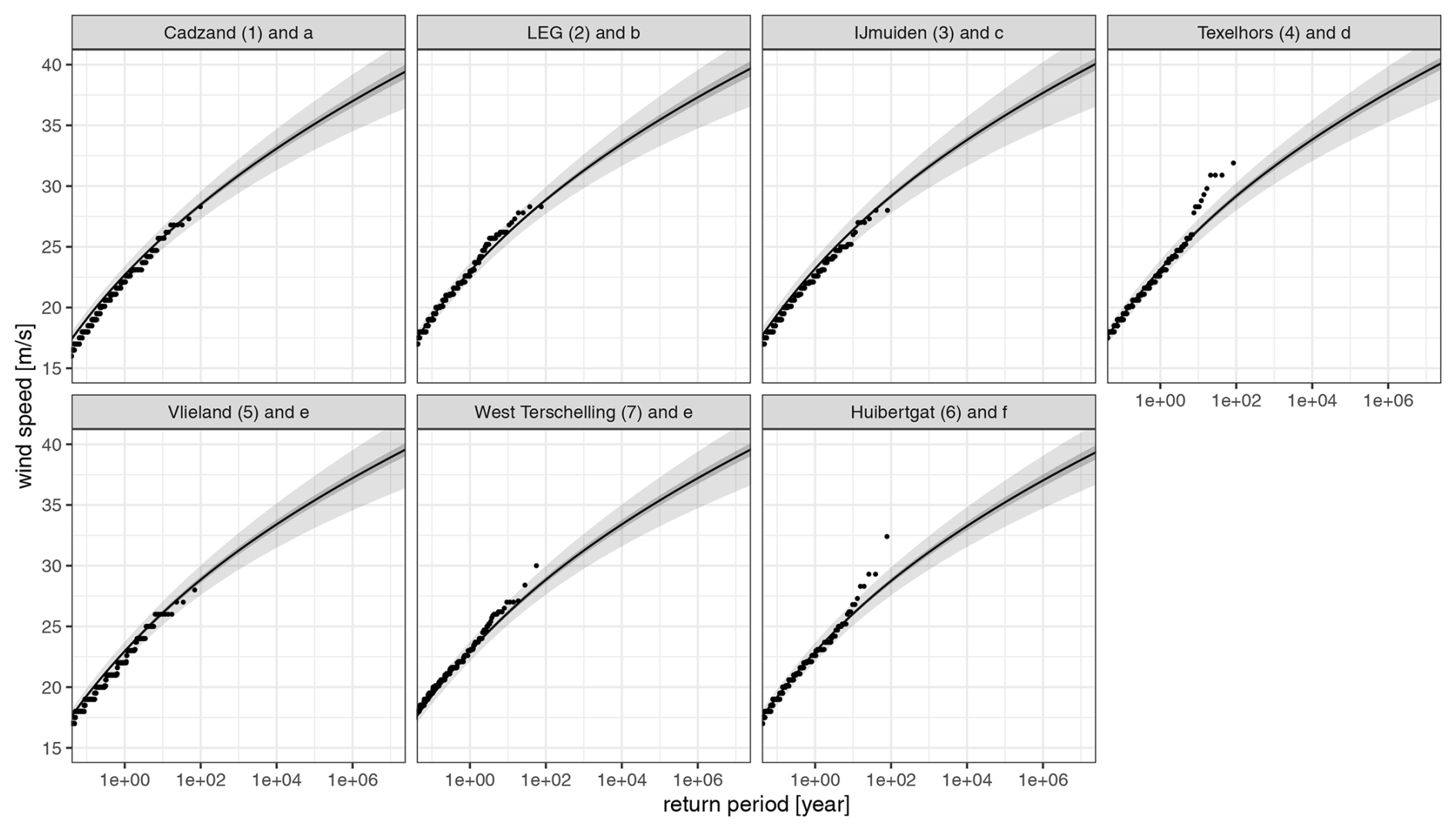
Figure 11 Empirical return values of wind speed u₁₀ restricted to wind directions from W to N from measurements at seven stations (dots; see headers) and corresponding provisional estimates derived from the corrected SEAS5 stress by the Charnock (0.025) relation, with sampling error (95 % confidence intervals, dark grey) and assessment of total uncertainty (95 % confidence intervals, light grey). Numbers and letters in the headers refer to the sites marked by squares and triangles in Fig. 1.

The estimates of the tails of stress (see Sect. S5) cannot be validated directly. As a sanity check, we compare the tail distributions of wind speed u₁₀ at a height of 10 m obtained from stress using an approximation formula to empirical distributions from measurement data. For the approximation, we use a logarithmic wind profile with roughness length z₀ determined from the Charnock relationship with a constant of 0.025, which agrees well with the corrected estimates from laboratory and field measurements in Curcic (2020) over the relevant wind speed range. The return values of wind speed associated with wind directions in the sector from W to N (which are not disturbed much by land) are compared with the empirical return values determined from hourly wind observations at nearby measurement stations; see Fig. 11. Here, the return period of the kth highest observation (circle) is determined as $L/\left(k\mathit{\alpha }\right)$, with L being the record length in years and $\mathit{\alpha }=\mathrm{1}/\mathrm{2}$ as above (this makes the comparison independent of the choice of the extremal index).

With the chosen Charnock constant, the overall agreement is surprisingly good. Had we chosen a lower Charnock constant, then we would have obtained return values for u₁₀ that markedly exceed the empirical values. For context, the value of 0.0185 as in Wu (1982) is commonly used in sea surface wave prediction models such as SWAN (Booij et al., 1999) to derive nearshore wave conditions from u₁₀. This indicates that the correction factor of 1.1 applied to the SEAS5 stress is not too low for simulating nearshore wave height and period for the purpose of estimating their return values (see Sect. 1).

The return values of wind speed u₁₀ for return periods above 100 years in Fig. 11 are not reliable, because they depend sensitively on the assumed Charnock relation; they are only shown to indicate the uncertainties in terms of wind speed.

The estimates of stress tails (Sect. S5) and of westerly to northerly wind speed tails in Fig. 11 show little variation along the coast, yet they appear to be consistent with measurement data. In fact, the most outlying observations in Fig. 11 are not particularly extreme and are each limited to a single site. Therefore, the large spatial variation in return values found in earlier analyses of wind measurements (Caires, 2009; Wieringa and Rijkoord, 1983) is likely due to sampling variability and possibly site-specific conditions such as spatial differences in roughness and topography.

6.3 High water

For high water (HW) at the six tide gauge stations (see Fig. 1), almost the same method is used as for stress, with one important difference: the scale yq^′(y) and location q(y) parameters of the GW tail Eq. (9) are estimated from the detrended measurement records, using a fixed shape parameter estimated from simulated HW data from the DCSMv5 model forced by SEAS5 stress and pressure gradient fields (see Sect. 2). This choice is based on the simulation study of de Valk and van den Brink (2023a), showing that scale and location can be estimated from relatively short records similar in size to the HW measurement records, if the shape is estimated from a record of the size of the local SEAS5 data.

Based on the estimates in Fig. 10 (right), the value of 1 was chosen for the extremal index: clustering of consecutive values of HW effectively vanishes with increasing threshold (decreasing sample fraction). We refer to Fig. 9 for an overview.

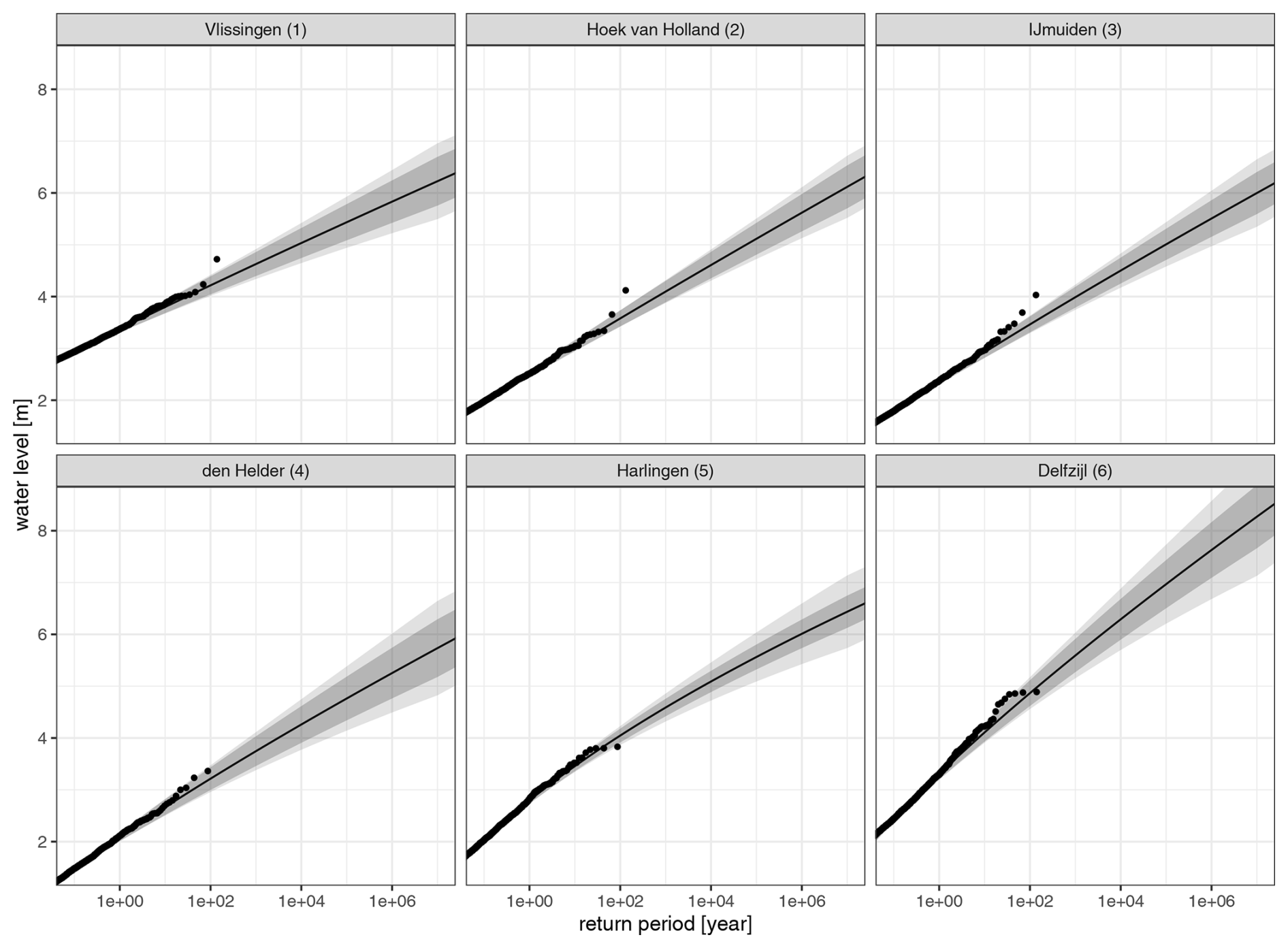
Figure 12 Estimated return values of water level at six tide gauge stations (see Fig. 1) with sampling error (95 % confidence intervals, dark grey) and assessment of total uncertainty (95 % confidence intervals, light grey), with empirical return values from tide gauge data (dots).

The estimated return values of HW are shown in Fig. 12 together with the empirical return values. The high values in Vlissingen (1), Hoek van Holland (2) and IJmuiden (3) reached during the severe 1953 flood stand out. For Hoek van Holland, this value has an estimated frequency of exceedance μ of 0.0011 yr⁻¹, so the probability that an annual maximum exceeds it in 132 years (the record length) is $\mathrm{1}-\exp (-\mathrm{132}\mathit{\mu })=\mathrm{0.14}$. Therefore, the 1953 water level is no outlier. Earlier estimates of the frequencies of exceedance from only measurements as in Dillingh et al. (1993) were higher, as the shape estimates were influenced by the high HW observed during the 1953 storm. By estimating the shape from simulated data, the present analysis avoids an overly large influence of single events.

As a further check, we compute for every station the ratio of the scale parameter estimated from tide gauge measurements and the scale parameter estimated from SEAS5/DCSMv5 data; see Table 1. If a bias in the tail of HW from SEAS5/DCSMv5 is only due to bias in the SEAS5 stress, then this ratio indicates the factor by which the SEAS5 stress should be corrected. The outlying value for Vlissingen can be explained by spatial mismatch: the DCSMv5 model has only a few output points in the small Western Scheldt (Westerschelde) estuary. The scale ratios for Hoek van Holland and IJmuiden along the west coast are close to the correction factor of 1.1 applied to the return values of stress, indicating that the ratios for these sites are to a large extent explained by bias in the SEAS5 stress. In fact, running the DCSMv5 model with SEAS5 stress fields inflated by a factor of 1.1 and repeating the analysis gives scale ratios which are 0.09 lower, which shows that the increase of the scale parameter of the tail of HW from the DCSMv5 model is almost proportional to the stress increase.

Table 1 Scale ratios (ratios of scale parameters of the tails of HW estimated with and without using measurement data for location and scale) for HW data simulated from SEAS5 stress and simulated from SEAS5 stress inflated by a factor of 1.1.

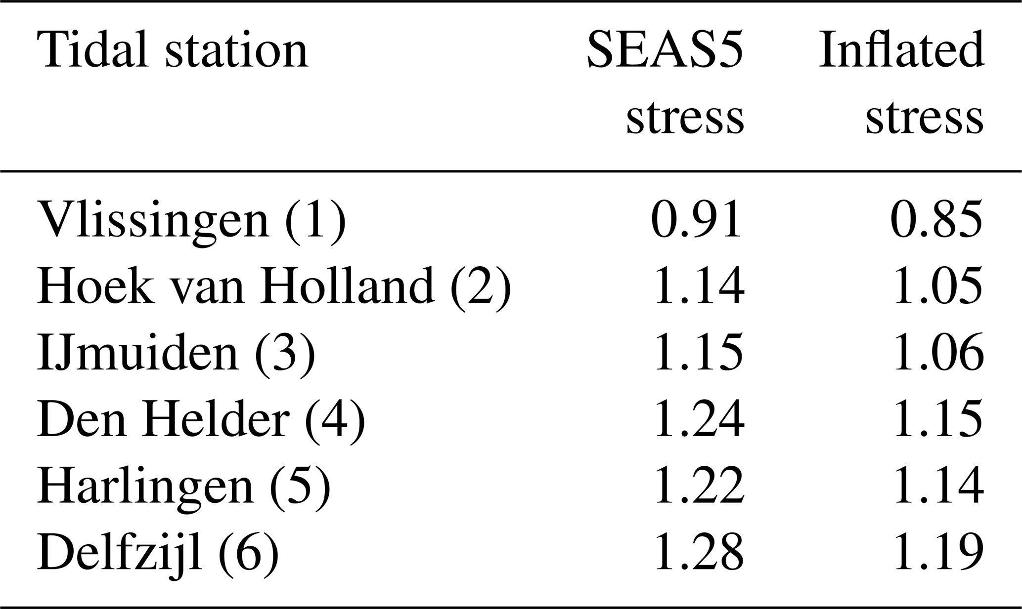
For the stations Den Helder (4), Harlingen (5) and Delfzijl (6) on the Wadden Sea estuary (Fig. 1), larger ratios are found. This could be due to errors in the stress forcing of the DCSMv5 model in this area (e.g. due to the limited resolution of SEAS5) or due to a bias in the DCSMv5 model when it is applied to this shallow estuary with complex bathymetry. A study of the effects of dynamic downscaling of the atmospheric forcing and of hydrodynamic model resolution (van den Brink, 2020) found no large systematic impact of resolution (see also Sect. 5). The current working hypothesis is therefore that under severe storm conditions certain process(es) in the shallow Wadden Sea are not adequately represented in current shallow-water flow models; investigating this further is beyond the scope of the present study.

6.4 Uncertainty of the estimates

We distinguish several sources of uncertainty. The sampling uncertainty, which is determined by the choice of the statistical model and the length of the dataset, is very small for stress and derived wind speed, as the stress tails are estimated from more than 8000 years of SEAS5 data. These uncertainties are shown in Fig. S6 (Sect. S5) for stress and in Fig. 11 for the speed of westerly to northerly wind u₁₀. For HW (Fig. 12), the uncertainties are larger than for stress and wind, as scale and location are estimated from relatively short records of tide gauge measurements, which widens the uncertainty ranges.

In addition, the error analysis should address model-related uncertainty: unknown systematic errors in the estimated tail distributions of wind shear stress and HW from simulated data resulting from limitations of the models such as limited resolution and parameterizations of processes which cannot be modelled based on first principles. We represent the model-related uncertainty in the GW tail distribution as a normally distributed error in the shape parameter. The reason for this choice is that errors in estimates of return values for large return periods are primarily determined by errors in the shape parameter. Furthermore, for HW, scale and location parameters are estimated from measurement data.

For shear stress from SEAS5, we assume that the model-related error in the shape parameter of the GW tail is normally distributed with mean of 0 and standard deviation of 0.1 (likely within ±0.1, very likely within ±0.2). The standard deviation is a crude estimate based on a comparison of estimates of the shape parameter γ (see Sect. 3.1) from annual maxima of SEAS5 stress and of the RACMOv2.3 downscaling of EC-Earth3 runs for the same area around the Netherlands (see Sect. 2), which differ considerably in resolution and drag relation; see Fig. 5. The mean difference over the southern and central North Sea is 0.026, from which we estimate the standard deviation by $\sqrt{(n-\mathrm{1}{)}^{-\mathrm{1}}{\sum }_{i=\mathrm{1}}^n(X_i-\widehat{\mathit{\mu }}{)}^{\mathrm{2}}}$ with n=2 as $\sqrt{{\mathrm{0.013}}^{\mathrm{2}}\times \mathrm{2}}=\mathrm{0.018}$. Using Eq. (8), this results in 0.12 (rounded to 0.1) for the standard deviation of the GW shape parameter of stress.

For HW, we employ the simplification that HW is roughly an affine function of stress (for small sample fractions, both in the hydrodynamic model and in reality; see Sect. 5), so the errors in the GW shape parameter of stress and HW are roughly equal. The model-related uncertainty is included as a random disturbance to the shape parameter estimates in the bootstrap procedure.

Confidence intervals of the resulting total error are shown as light grey bands in Fig. S6 (Sect. S5) for stress, in Fig. 11 for the speed of W to N wind u₁₀ provisionally derived from stress and in Fig. 12 for HW. The dark grey bands are the intervals based on sampling errors only. In particular for stress and derived wind, the model-related error broadens the intervals considerably.

For HW, we can evaluate the effect of the use of simulated data on the total uncertainty of return value estimates for a return period of 10⁷ years. Table 2 (first column) shows for each station the ratio of the standard deviation of the estimate from measurements to the standard deviation of the estimate partially based on simulated data. The estimates are both based on GW tail fits (Sect. 3) using thresholds exceeded by the same sample fraction of 0.012, so the factors represent only the reduction in total uncertainty due to the use of simulated data for shape estimation. The average reduction is by a factor of 2.4. The second column shows the reduction factor relative to the standard deviation of GP tail fits to measurements only. These numbers are considerably higher: on average 5.1. This shows that both the use of simulated data to estimate shape and the choice for a GW tail instead of the more conventional GP tail can contribute substantially to the reduction of the uncertainty in return value estimates. This is qualitatively in line with simulation results in de Valk and van den Brink (2023a).

Table 2 Reduction factors in total uncertainty (standard deviation, including mode-related uncertainty) achieved by using the new 10⁷-year return value estimates for HW instead of GW tail fits to measurement data only (left) or GP tail fits to measurement data only (right).

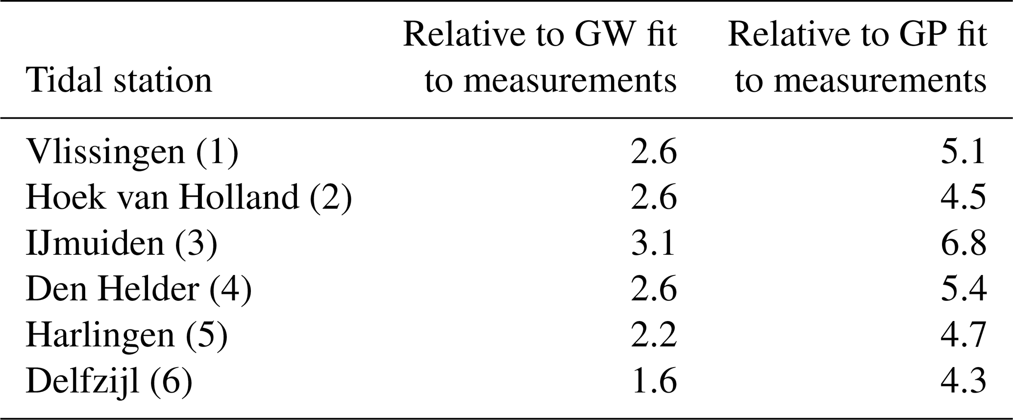
The reduction factors in Table 2 are not accurate: it is difficult to assess the uncertainty of return value estimates from measurements reliably (see Sect. S1), and our assessment of the model-related error in shape estimates from simulated data is crude.

7 Conclusions and outlook

Even a measurement record of about 140 years (considered long in meteorology) is not enough to reasonably constrain return values for large return periods of 10 000 years or higher. This case study demonstrates that the uncertainty in the statistical modelling of extreme coastal water level can be reduced considerably by the cautious use of large archives of weather data simulated by state-of-the-art models and water levels simulated from these data (Sects. 4–6).

The uncertainty in the 10⁷-year water level is reduced by a factor of 2.4 on average (Table 2). This is achieved by estimating the tail shapes from about 8000 years of simulated data. We substantiate that these shape estimates are reliable (Sects. 4–5); for stress, they show very little dependence on model resolution and drag formulation, and shape estimates are generally compatible with estimates from measurements or reanalysis data. Our uncertainty assessment includes the model-related error (Sect. 6.4).

The reduction in uncertainty is modest compared to the potential reduction of typically $\sqrt{\mathrm{8000}/\mathrm{140}}=\mathrm{7.6}$ for a measurement record of 140 years. Further reduction toward this limit is possible if it can be shown that the model-related error in tail shape is smaller than our current estimate and/or if models improve so much that the scale and location parameters can be reliably estimated from simulated data. Furthermore, if the biases in location and scale estimates derived from simulated data are spatially smooth, this smoothness may be exploited to reduce the estimation error further (e.g. Wood et al., 2016; Wood, 2020; Calafat and Marcos, 2020). Table 1 indicates that this is a reasonable assumption, except for Vlissingen on the narrow Western Scheldt (Westerschelde) estuary where model resolution is insufficient.

The choice of the type of tail distribution to be fitted to the data also matters. We use the generalized Weibull (GW) tail (Sect. 3). When we compare the uncertainty of our estimates of the 10⁷-year water level to the uncertainty of estimates obtained by the conventional method of fitting a generalized Pareto (GP) tail to measurements only, we find an average reduction by a factor of 5.1 (Table 2). This shows that both the use of simulated data to estimate shape and the choice for a GW tail instead of the more conventional GP tail can contribute substantially to the reduction of the uncertainty in return value estimates.

Furthermore, the use of simulated weather data makes it possible to estimate return values of stress, which is not measured. This is important for flood risk assessment, as stress constitutes the main link between atmospheric dynamics, storm surge and sea surface waves. Return values of stress from the simulated data are corrected by a factor of 1.1, in reasonable agreement with the HW scale parameter corrections for tidal stations on the west coast in Table 1, as well as with wind measurements when assuming a Charnock constant of 0.025 (see Fig. 11).

A side effect of the use of very large simulated datasets in this study is that return value estimates are spatially smooth and insensitive to individual events such as the 1953 storm. Dependencies between variables in the extreme ranges of stress and HW such as wind-direction-dependent return values and dependence between stress and HW are not discussed here. Elsewhere in de Valk and van den Brink (2023b), it is shown how simulated data can be used to improve the estimation of dependencies.

The present method, developed for the Dutch coast, may be applicable to other coastlines along the North Sea and possibly to other regions with similar climates and to other variables. However, careful review and checking of the assumptions and their consequences for the application is essential. A potential advantage of very large archives of simulated weather is good coverage of the phase space, but this will only materialize if all relevant phenomena (e.g. storm types) are faithfully represented in the simulated data.

In the present study, estimates of return values of HW from simulated data are corrected based on a tail fit from measurement data which uses the shape estimate from the simulated data. As only the scale and location parameters are adjusted, this correction is affine. If the tail shape remains the same in a changing climate, then the same affine correction may be applied to correct the bias in return values from simulations based on different scenarios of future climate forcing. However, the assumption of a constant shape may not be valid, e.g. under scenarios in which new extreme populations emerge such as post-tropical cyclones (e.g. Baatsen, 2015; Sainsbury et al., 2020). This requires that (changes in) the shapes of tails associated with relevant populations are examined separately, which is a topic for future research.

Appendix A: Glossary

High water (abbrev. HW)	the maximum height reached during a rising tide (including the meteorologically forced contribution) relative to a fixed datum (Hicks, 1989) (also hoogwaterstand (Dutch), Hochwasserstand (German))
Skew surge	the difference between the high water and the astronomical high water predicted for the same cycle
Return value	the value exceeded with a given frequency $\mathit{\mu }=\mathrm{1}/T$, with T being the return period in years
Sampling error	the uncertainty in an estimate from a data sample due to unexplained variation in the values within the sample
Affine	an affine transformation is a transformation consisting of a linear transformation and a translation