Evaluation of machine learning approaches for large-scale agricultural drought forecasts to improve monitoring and preparedness in Brazil

​​​​​​​Drought events have increased in frequency and severity in recent years and result in significant economic losses. Although the Brazilian semi-arid Northeast has been historically associated with the impacts of drought, drought is of national concern. From 2011–2019, drought events were recorded in all Brazilian territories. Droughts can have major consequences for agricultural production, which is of particular concern given the importance of soybeans for socio-economic development. Due to its regional heterogeneity, it is important to develop accurate drought forecast and assessment tools for Brazil. We explore machine learning as a method to forecast the vegetation health index (VHI), for large-scale monthly drought monitoring across agricultural land in Brazil. Furthermore, we also determine spatio-temporal drivers of the VHI across the wide variation in climates and evaluate machine learning performance for El Niño–Southern Oscillation variation and forecasting of the onset of drought stress. We show that machine learning methods such as gradient boosting methods are able to more easily forecast vegetation health in north and northeast Brazil than in south Brazil, and they perform better during La Niña events than El Niño events. Drought stress which reduces the VHI below the commonly used 40 % threshold can be forecast across Brazil with similar model performance. The standardized precipitation evapotranspiration index is shown to be a useful indicator of drought stress, with 3-month accumulation periods preferred over 1- and 2-month periods. Results aim to inform future developments in operational drought monitoring at the National Centre for Monitoring and Early Warning of Natural Disasters in Brazil (CEMADEN). Future work should build upon methods discussed here to improve drought forecasts for agricultural drought response and disaster risk reduction.

1 Introduction

Drought events have increased in frequency and severity in recent years and can result in significant economic losses (Cunha et al., 2019; Herweijer and Seager, 2008; Marengo et al., 2017; Brito et al., 2018). According to a 2020 United Nations report, drought caused at least USD 124 billion in economic losses and affected more than 1.5 billion people from 1998 to 2017. Furthermore, 5 billion people will live in water-scarce areas by 2050 (Brodribb et al., 2020; Wei et al., 2024). Meteorological droughts are defined as an extended period in which a water deficit occurs, usually because precipitation is less than average, resulting in water scarcity (Cunha et al., 2019). Droughts can have significant consequences for sectors, including drinking water supply, waterborne transportation, electricity production, and agriculture (Van Loon, 2015). Agricultural drought is defined as the point at which drought conditions result in adverse plant responses such as crop failure (NOAA, 2024).

Agricultural drought can have significant socio-economic impacts because they impact food security. For example, droughts reduced European cereal yields by 9 % on average between 1961 and 2018 (Brás et al., 2021). Sensitivity to drought effects can depend on management factors such as crop selection, irrigation, and tillage practice, as well as climate variability (Wilhelmi and Wilhite, 2002). Agricultural drought has been effectively detected using the vegetation health index (VHI), a proxy for the estimation of vegetation health (Kogan, 2002; Wu et al., 2020). This is because the VHI, from AVHRR (Advanced Very High Resolution Radiometer) data, responds cumulatively and quickly to changes in vegetation greenness. Therefore, the effect of drought can be measured much earlier than that derived from weather data or other drought monitoring tools, which allows for faster adaptation responses (Kogan, 2002). Drought monitoring using vegetation indices such as the VHI, the NDVI (normalized difference vegetation index), or the VCI (vegetation condition index) has been developed in several locations using satellite imagery from products such as MODIS and NOAA STAR (Sadiq et al., 2023; Kloos et al., 2021). The VHI is defined as the weighted average of two subindices: the VCI and the temperature condition index (TCI). A full definition of the VHI is found in Sect. 2.2.1. Although partly based on the NDVI, the VHI is reported to improve upon using the NDVI for drought monitoring as it provides a measure of vegetation condition relative to long-term change (West et al., 2019). Although monitoring past events is useful, a forecasting method would be highly beneficial to provide timely warnings of drought intensification to government officials and other stakeholders.

Machine learning has been shown to outperform and hold many advantages over traditional statistical and time-series-based prediction methods; in particular machine learning can more easily capture non-linear relationships and does not assume a certain shape of the response function (Leng and Hall, 2020). Machine learning has been used to forecast vegetation indices at timescales including daily, 5 d, and 7 d intervals (Kartal et al., 2024; Kladny et al., 2024; Reddy and Prasad, 2018); monthly intervals (Lees et al., 2022); weekly timescales (Barrett et al., 2020); and average vegetation condition values aggregated over 1–3 months (Adede et al., 2019). Models used to predict the VHI range from neural networks (Adede et al., 2019; Kladny et al., 2024; Lees et al., 2022; Reddy and Prasad, 2018) to ensemble tree methods such as random forest and gradient boosting methods (Nay et al., 2018; Tanguy et al., 2023), with some studies using other methods such as Gaussian process modelling (Barrett et al., 2020). Results from many such studies show the potential of machine learning and remote sensing indices to effectively forecast agricultural drought. For example, Nay et al. (2018) used gradient boosting methods to forecast the enhanced vegetation index (EVI) and demonstrated correlations in agricultural areas between the modelled and the observed EVI above 0.75. Furthermore, Lees et al. (2022) evaluated forecasts of the VCI in Kenya made with neural networks and deep learning LSTM (long short-term memory) methods and found excellent performance. This work showed that forecasting the VCI 1 month in advance with an LSTM model can achieve an R² value of up to 0.83. Other work has also shown impressive results, suggesting great potential for machine learning methods to forecast drought impacts on the VHI at a large scale.

In Brazil, drought accounts for approximately half of natural-disaster-related impacts in terms of the number of people affected (Sena et al., 2014). Droughts are of particular concern in the northeast semi-arid region, one of the most densely populated semi-arid regions in the world, which also has the most people living in poverty in Brazil. Nearly 80 % of agricultural labour in the northeast is smallholder farmers, and rainfed agriculture accounts for 95 % of farmed land (Cunha et al., 2019; Marengo et al., 2022). Much work has focused on drought trends in Brazil, with particular focus on the northeast semi-arid region (Cunha et al., 2019; Marengo et al., 2017, 2022; Rossato et al., 2017; Zeri et al., 2018). However, in recent years, drought impacts have affected all regions in Brazil (Cunha et al., 2019; Tomasella et al., 2023). For example, in 2020 drought in Rio Grande do Sul was estimated to have cost BRL 36 billion (∼ USD 6.22 billion) in losses, representing 7.36 % of the state's GDP (CNA, 2020). Drought has also been linked to inflation, reportedly causing an increase in food prices of 8.03 % in 2014 (Agência Brasil, 2015). Due to its regional heterogeneity, it is important to develop accurate drought forecast and assessment tools for all of Brazil (Cunha et al., 2019). Drought monitoring and dissemination of drought warnings and intensification in Brazil is undertaken by the National Centre for Monitoring and Early Warning of Natural Disasters (CEMADEN). CEMADEN uses several drought indices including the standardized precipitation index (SPI), root zone soil moisture (RZSM) from remote sensing, and vegetation indices based on remote sensing such as the vegetation health index (VHI). These variables are part of an integrated drought index (IDI), which takes into account classified versions of these products, harmonized to a common spatial resolution and domain. The publicly available IDI is then used to make the diagnostic of current drought conditions over all regions of the country but is not used to forecast drought metrics. This helps to inform stakeholders of ongoing drought events across the country. In this study, we aim to build on the drought monitoring work at CEMADEN by assessing the potential of machine-learning-based operational drought impact forecasting at monthly timescales using satellite-based VHI observations and drought indices at a large scale across Brazil.

In summary, the objectives of this study are the following:

1. to determine the effectiveness of machine learning methods for VHI forecasts at monthly timescales across agricultural areas of Brazil

2. to determine which input variables are most useful for drought forecasting models when used across Brazil

3. to determine the effectiveness of machine learning methods for forecasting the onset of VHI drought

4. to determine how El Niño–Southern Oscillation (ENSO) modes of variation affect VHI forecast performance.

2 Methods and data

2.1 Study area

Brazil contains a wide variety of climate conditions and geographic features which present a challenge for prediction when training and evaluating model performance across such a wide area. Spatial variation in climate is particularly significant in Brazil. The climate of Brazil is made up of  nine different Köppen–Geiger climate zones from semi-arid in the northeast to tropical savanna and tropical rainforest in the northwest, with some areas of marine climate in the south (Peel et al., 2007; Beck et al., 2018). In addition to climate zones, a wide variety of different biomes are found across the country. Biomes in Brazil have been defined as Amazon, Atlantic Forest, Caatinga, Cerrado, Pampa, and Pantanal (Lopes Ribeiro et al., 2021). The Amazon biome is mainly characterized by rainforest areas and has an equatorial climate with torrential rains distributed throughout the year (Overbeck et al., 2015; Lopes Ribeiro et al., 2021). Atlantic Forest is characterized by heavy rainfall due to the proximity to the ocean and winds blowing inward over the continent (Lopes Ribeiro et al., 2021). The Caatinga biome experiences high temperatures and potential evapotranspiration rates that exceed 2500 mm yr⁻¹. This leads to the characterization of the Caatinga as being of low water availability and having limited storage capacity of rivers (Lopes Ribeiro et al., 2021). The Cerrado is characterized by large savannahs with a warm tropical subhumid climate and two distinct seasons: wet summers with torrential rains and dry winters (Overbeck et al., 2015; Lopes Ribeiro et al., 2021). The Pampa biome, located in the south, has a wet subtropical climate and is rainy throughout the year with hot summers and cold winters. Pantanal is made up of poorly drained lowlands which experience flooding from summer to autumn months. Precipitation varies from 1000 to 1400 mm yr⁻¹ (Ioris et al., 2014; Lopes Ribeiro et al., 2021). All input and output data were filtered using harvested areas from the crop grid dataset (Tang et al., 2023). The crop grid (Tang et al., 2023) dataset was chosen because it is the newest dataset found with estimates of the crop-specific growing area for maize and soybeans in Brazil. The data were filtered to only contain grid cells which are above the 75th percentile of harvested area across the distribution of the maize and soybean harvested area in Brazil. This is to ensure that the grid cells used for training and evaluation are most likely to be indicative of cropland for two major crops grown in Brazil: soybean and maize. Choosing maize and soybean growing areas provides a large spread across different climatic zones of Brazil and ensures representation of two crops with economic and food security value. As an additional test, models were also trained using maize and soybean growing areas separately. The results of this test are found in Appendix D. Figure 1 shows the spatial distribution of soybean (Fig. 1a) and maize (Fig. 1b) growing areas.

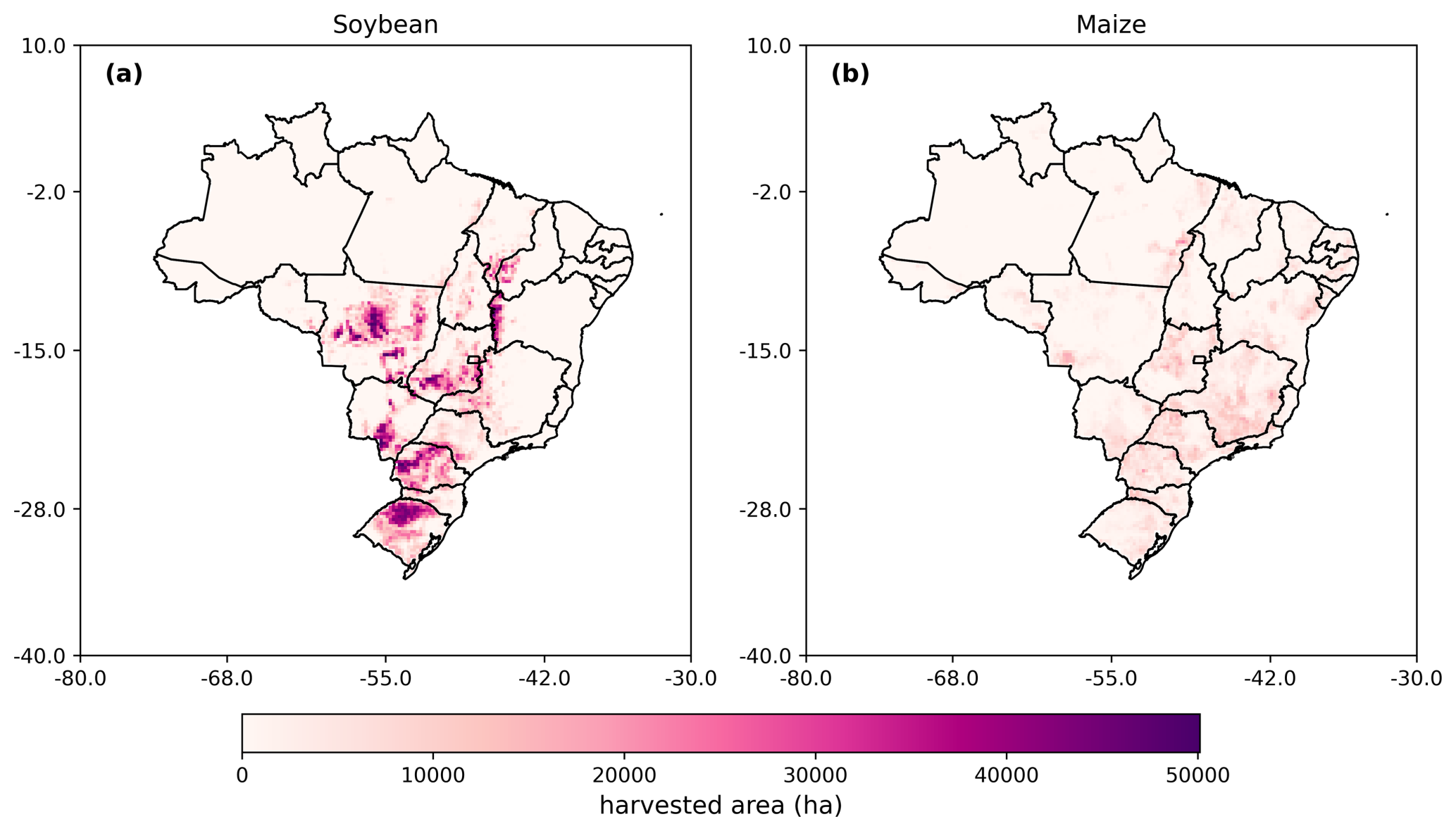
Figure 1 Maps of harvested areas (circa 2020) across Brazil taken from the crop grid database. Panel (a) shows the soybean harvested area. Panel (b) shows the maize harvested area.

Using the approach here to select for regions, the cropland area was obtained for a range of locations across Brazil. Much of the most intensely farmed soybean area is in the state of Mato Grosso in central Brazil, Rio Grande do Sul and Paraná in the south, and some locations in Bahia in the northeast. Maize is farmed much less intensively than soybeans, but it is equally widespread throughout the country. More maize is grown in Minas Gerais than soybean and is more widespread in the northeast of the country.

The large spatial scale of this work makes model training particularly challenging. Agricultural land in Brazil is made up of multiple biomes with different soil moisture, rainfall, and temperature characteristics (Cunha et al., 2019; Lopes Ribeiro et al., 2021). Meteorological events such as ENSO also affect different parts of the country in different ways. Typically, during El Niño events, there is a reduction in precipitation in the north and northeast regions, while the south experiences a higher frequency of heavier rains. In La Niña events, the situation is reversed, with the north and northeast experiencing greater-than-average rainfall and the south being subjected to more severe droughts (Cirino et al., 2015).

2.2 Input variables and drought indices

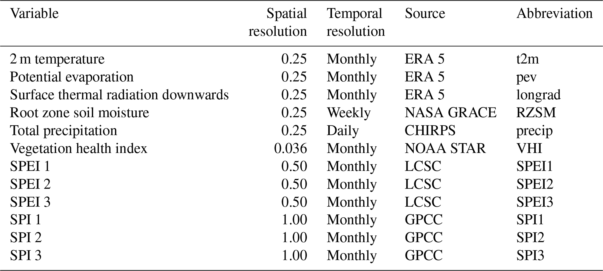
Drought indices were taken from a range of sources, resampled to ensure consistent spatial and temporal resolution (see Sect. 2.3), and then assimilated to create a combined dataset to describe drought conditions across Brazil at 0.25° spatial resolution for each month. To obtain consistent dates across data sources, the dataset ranges from 2003 to 2022. These years also account for seasonal variability and cyclical climate processes, including ENSO, which is addressed in this study.

2.2.1 Vegetation health index (VHI)

The vegetation health index is a proxy for estimating overall vegetation health and is expressed in percentage. VHI values below 40 % indicate stress conditions. The VHI is a composite index which is comprised of the vegetation condition index (VCI) and the TCI. These three variables are determined by the following formulae:

$$\begin{array}{}\text{(1)}& {\displaystyle }\mathrm{VCI}={\displaystyle \frac{\mathrm{100}(\mathrm{NDVI}-{\mathrm{NDVI}}_{min})}{{\mathrm{NDVI}}_{max}-{\mathrm{NDVI}}_{min}}}\text{(2)}& {\displaystyle }\mathrm{TCI}={\displaystyle \frac{\mathrm{100}({\mathrm{BT}}_{max}-\mathrm{BT})}{{\mathrm{BT}}_{max}-{\mathrm{BT}}_{min}}}\end{array}$$

$$\begin{array}{}\text{(3)}& \mathrm{VHI}=\mathit{\alpha }\mathrm{VCI}+(\mathrm{1}-\mathit{\alpha })\mathrm{TCI},\end{array}$$

where BT is the brightness temperature recorded from a thermal sensor, min/max represents minimum and maximum values of a variable over the study period, and α is a coefficient used to determine the relative contribution of the TCI and the VCI to the VHI. The vegetation health index data were obtained from the NOAA STAR satellite-based vegetation health system. The NOAA STAR system uses data and products from GOES (Geostationary Operational Environmental Satellite), METEOSAT, MTSAT, and DMSP. Satellite observations are primarily based on radiance measurements taken by the Advance Very High Resolution Radiometer (AVHRR) found on NOAA polar-orbiting satellites. The visible and infrared observations are used to determine the NDVI as well as the TCI, the VCI, and the vegetation health index (VHI) (Kogan, 1997). VHI data were obtained at the resolution of 0.036° (4 km) but then were upscaled to 0.25° to bring them to the common spatial resolution of the majority of the input data.

2.2.2 Soil moisture

Soil moisture is essential to measure the propagation of meteorological drought into agricultural drought and water stress in plants (Zeri et al., 2018, 2022). In this work, soil moisture was obtained from the NASA GRACE satellite (Li et al., 2019). The NASA GRACE satellite data are based on two satellites which record changes in the earth's gravity field caused by the redistribution of water. Root zone soil moisture was obtained from GRACE for the 0.25° grid scale and a weekly timescale. Temporal resolution was reduced to monthly by averaging soil moisture percentage across 4-week intervals.

2.2.3 Standardized precipitation index (SPI)

The standardized precipitation index (SPI) is a drought index with wide comparability for different locations due to spatially consistent standardization. This makes the SPI a useful index for constructing a model of drought propagation across such a wide spatial domain as agricultural land in Brazil. The SPI was first proposed by McKee et al. (1993) to quantify the probability of occurrence of a precipitation deficit at a particular monthly timescale. To determine the SPI, precipitation data are fitted to a probability distribution function (usually either gamma or Pearson), before the inverse normal distribution function is used to rescale probability values, leading to SPI values with a mean of zero and standard deviation of 1 (Cunha et al., 2019). The SPI is calculated over different monthly timescales. Here, we use 1-, 2- and 3-month SPIs. Various studies have shown that SPI3 has the strongest correlation with vegetation response (Sepulcre-Canto et al., 2012); however, we also assess 1- and 2-month accumulation periods, which may also be useful for dry environments (Tanguy et al., 2023). SPI indicators with longer accumulation periods are not part of the main model results for reasons provided in Appendix E. The SPI is a widely used index recommended by the World Meteorological Organization (WMO). It is also used for operational drought monitoring at CEMADEN (Cunha et al., 2019).

SPI data were taken from the NOAA–NIDIS Global Precipitation Climatology Centre (GPCC) (Ziese et al., 2011). We selected SPI data fit to a gamma distribution. Data were obtained at a 1° resolution and then upsampled using a k-nearest neighbours algorithm to obtain a consistent spatial resolution with the rest of the dataset at 0.25°.

2.2.4 Standardized precipitation evapotranspiration index (SPEI)

The SPEI (standardized precipitation evapotranspiration index) was first proposed by Vicente-Serrano et al. (2010) as an improved drought index which considers the effect of reference evapotranspiration on drought severity. The SPEI is based on the calculation of the SPI; however, the SPEI is determined by computing a climatic water balance (precipitation minus atmospheric evaporative demand) and then using this metric to determine the probability of a water balance deficit for a given period of time (Beguería et al., 2014). Similar to the SPI, a statistical distribution is then used to fit the data, and the data are standardized to produce a mean of zero and standard deviation of 1 (Beguería et al., 2010).

SPEI data were taken from the global SPEI database (SPEIbase), which was originally at a 0.5° spatial resolution (Beguería et al., 2010). Beguería et al. (2010) use a log-logistic distribution to fit the SPEI. The SPEI is an advancement on the SPI (standardized precipitation index) because the incorporation of evapotranspiration effects accounts for temperature effects on drought, which have been shown to significantly affect drought conditions (Rebetez et al., 2006). SPEI values are determined for a number of months, termed accumulation periods. Different accumulation periods could be more useful for specific representations (e.g. longer accumulation periods could be more correlated with longer-term storage effects such as groundwater). Here, we assess 1–3-month accumulation periods for consistency with SPI accumulation periods and relevance to crop growth periods.

2.2.5 ERA5 reanalysis input variables

Further data were obtained from the monthly averaged ERA5 database (Hersbach et al., 2023). ERA5 is a reanalysis database which combines models and observations using data assimilation to provide better estimates of meteorological variables at the grid scale (Hersbach et al., 2023). Although ERA5 has an hourly global coverage, we use monthly averaged estimates to allow for consistency with the rest of the data used for this study.

From this resource, 2 m temperature, potential evaporation, and surface thermal (longwave) radiation downward were obtained. Temperature variables are important to capture drought effects brought on by high temperatures rather than solely a deficit in rainfall. This can be especially important for flash drought events, which are typically caused by the compounding effects of rainfall deficits and high temperatures, which increase evaporative stress (Christian et al., 2021).

2.2.6 Total monthly precipitation

Precipitation data were obtained from the Climate Hazards Group InfraRed Precipitation with Station data (CHIRPS) database (Funk et al., 2015). CHIRPS is a quasi-global database (ranging from 50° N–50° S) which is available at multiple spatial resolutions including 0.25°. The CHIRPS dataset combines satellite data with in situ measurements to provide a gridded dataset of appropriate spatial extent for this study. CHIRPS has been validated against other datasets and in situ observations and has been used for similar studies in other regions (Lees et al., 2022). Total monthly precipitation is included as a variable to provide a benchmark comparison to precipitation indices when analysing variable importance.

2.3 Data processing and sampling methods

Data were originally obtained at a range of different spatial and temporal resolutions. Table 1 shows the original resolution of each of the indices used. Where spatial resolution has been decreased (spatial down sampling), this is done through averaging. Where spatial resolution has increased (spatial up sampling), this is calculated using a k-nearest neighbours algorithm (where k is the five nearest neighbours). All data were spatially corrected to a 0.25° spatial resolution. Some data were obtained at weekly or daily timescales; in this case, data were averaged per month for each grid cell location to obtain average monthly estimates of each variable.

Table 1 Variables considered for use in this study with original spatial (degrees) and temporal resolutions, sources, and abbreviations used in this paper. LCSC – Climatology and Climate Services Laboratory.

2.4 Forecasting methods

We evaluate a range of machine learning methods for the forecasting of the vegetation health index 1 month in advance before using the best model to assess the performance of further forecasts aimed at predicting the vegetation health index 2 and 3 months in advance and more closely analysing spatio-temporal model performance. Methods compared here are random forest (Breiman, 2001), gradient boosting (Friedman, 2001), artificial neural networks (LeCun et al., 2015), k-nearest neighbours regression (KNR), ridge regression, and a multiple linear regression for comparison.

Random forest and gradient boosting are tree-based methods which construct an ensemble of decision trees. Decision trees partition data into subsets based on conditions at each leaf node of the tree. Tree depth and complexity can be specified by the user. Random forest constructs a specified number of trees and then averages the result of each individual tree. Different trees are trained on different randomized subsamples of the dataset, a method known as bootstrapping. Gradient boosting methods differ from random forest in that decision trees are trained sequentially rather than simultaneously, with residual error from previous decision trees used to improve each subsequent model (Friedman, 2001; Breiman, 2001; Marsland, 2011).

Artificial neural networks are layered networks of inter-connected units which each contains a set of weights. Weights are optimized against an error term and the training data using a separate optimization algorithm. Deep neural networks are those which contain many subsequent processing layers (LeCun et al., 2015). Neural networks are flexible architectures, with many adaptations being constructed for different tasks. Here, we compare a fully connected neural network. Fully connected neural networks are named as such because each node in the preceding layer is connected to each node in the subsequent layer.

The k-nearest neighbours regression is a semi-supervised learning method which uses a user-defined k value to learn the k-nearest data based on a distance calculation. Most commonly this method uses the Euclidean distance metric for this approach; however, other distance metrics may be used (Chomboon et al., 2015). Multiple linear regression and ridge regression are used as linear comparisons to more complex methods used here to assess the appropriate level of complexity for the model required.

A comparison is also made between each of the above-described models and a seasonal average model (denoted SEA AV). The seasonal average model is simply the average value of the VHI for a particular location and month. The purpose of this model is to provide a low benchmark comparison to assess model performance relative to that which would be achieved by simply using the seasonality of the VHI alone.

2.5 Cross-validation and training procedure

We cross-validated models across a large span of years to provide a general picture of model performance regardless of evaluation period. Evaluation was split by year to avoid the influence of spatial autocorrelation on data leakage between training, validation, and testing splits. Model evaluation metrics were obtained by training 10 separate models with the same set of hyperparameters each tested using a randomized hold-out test year. Results for each model are then aggregated to produce metrics across the 10-year aggregation period. Furthermore, we also evaluated optimal hyperparameter values, the results of which can be found in Appendix A. To optimize hyperparameters, the data were again split by year to avoid any shared information between splits; however, data were also split three times into training, validation, and testing. For this method, we used a hold-out evaluation dataset of 5 random years. These years were chosen as 2006, 2011, 2015, 2016, and 2019. The rest of the data are split between two randomized folds based on year. The best set of hyperparameters across both folds is used to train each model before subsequent testing on the evaluation dataset. The decision was made to train and evaluate on as much data as possible here with suboptimal parameters to provide the best indication of general model performance across a wider range of evaluation years. This allows us to better look into effects of ENSO on model performance and inter-annual variability regardless of specific hyperparameter optimization. Although hyperparameter optimization did change the results of individual models slightly, the best model was the same across both training and evaluation procedures. Furthermore, it was found that the best model results were achieved by simply training on more data, rather than a specific set of hyperparameters.

2.6 Model evaluation methods

Model performance is evaluated using complementary mean absolute error and coefficient of determination metrics (R²). Coefficient of determination is used to determine the performance of the model against a wide degree of variability, with a high coefficient of determination indicating that the model captures both extremes at the low and high end of the distribution.

2.6.1 Drought onset forecasting evaluation

Furthermore, prediction of the onset of drought impact is evaluated in Sect. 3.4. Here, we use precision and recall as metrics for evaluating whether the model correctly predicts when the VHI decreases below 40 %. The 40 % threshold is chosen because it is used in many drought monitoring systems as the critical threshold at which warnings are issued (Kogan, 1997; Kogan et al., 2013; Gidey et al., 2018). Recall and precision are defined by the four classification metrics used to determine classification performance: true positives (TPs), true negatives (TNs), false positives (FPs), and false negatives (FNs). A true positive is determined when the observed value of the VHI falls below 40 %, and the model correctly forecasts a value of the VHI below 40 % for that month. Conversely, if the observed value of the VHI falls below 40 % but the model forecasts a value above 40 %, this is a false negative. Likewise, if the model forecasts a value below 40 %, which was not observed, this is classed as a false positive. Finally, if both the observed and predicted values fall above the 40 % threshold, a true negative is determined. Table 2 defines each of the classification values.

Table 2 Definitions of classification metrics used to determine model performance for accurately predicting the onset of drought impacts on the VHI.

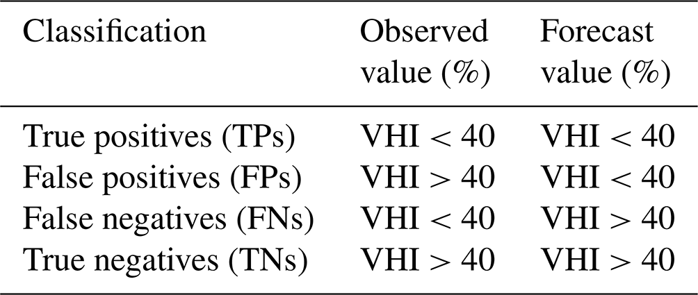
Recall and precision are defined using the classification determined in Table 2. Recall is a measure of the number of true positives as a ratio of the number of true positives plus the number of false negatives. Formally, recall is defined as

$$\begin{array}{}\text{(4)}& \mathrm{recall}={\displaystyle \frac{\mathrm{TP}}{\mathrm{TP}+\mathrm{FN}}}.\end{array}$$

In this manner, recall can be thought of as the performance of the model in proportion to the bias towards predicting the negative class (values above 40 %). Precision is similarly defined as

$$\begin{array}{}\text{(5)}& \mathrm{precision}={\displaystyle \frac{\mathrm{TP}}{\mathrm{TP}+\mathrm{FP}}}.\end{array}$$

Precision is therefore defined as the number of true positives as a ratio of the number of true positives plus the number of false positives. It can therefore be thought of as the performance of the model in proportion to the bias towards predicting the positive class (values below 40 %).

3 Results

The results of this paper aim to present a first look at the potential of machine learning to produce monthly VHI forecasts and the impacts of drought on the VHI across Brazil. Model performance indicates great benefit can be obtained from forecasting subseasonal vegetation health 1 month in advance. Forecasts further in advance, for 2 and 3 months, may also be achievable but show much greater model uncertainty with methods tested.

3.1 Drivers of VHI variability

Figure 2 shows the correlations between the SPI and the SPEI with the vegetation health index of the following month. Longer accumulation periods lead to greater correlations with the VHI. SPEI values are more strongly correlated with VHI values in some regions than the SPI. Regions where this occurs include northern Mato Grosso in central Brazil and the south. Neither the SPEI nor the SPI has a very strong correlation with next month's VHI in these regions, but the SPEI typically has correlations which are less weak.

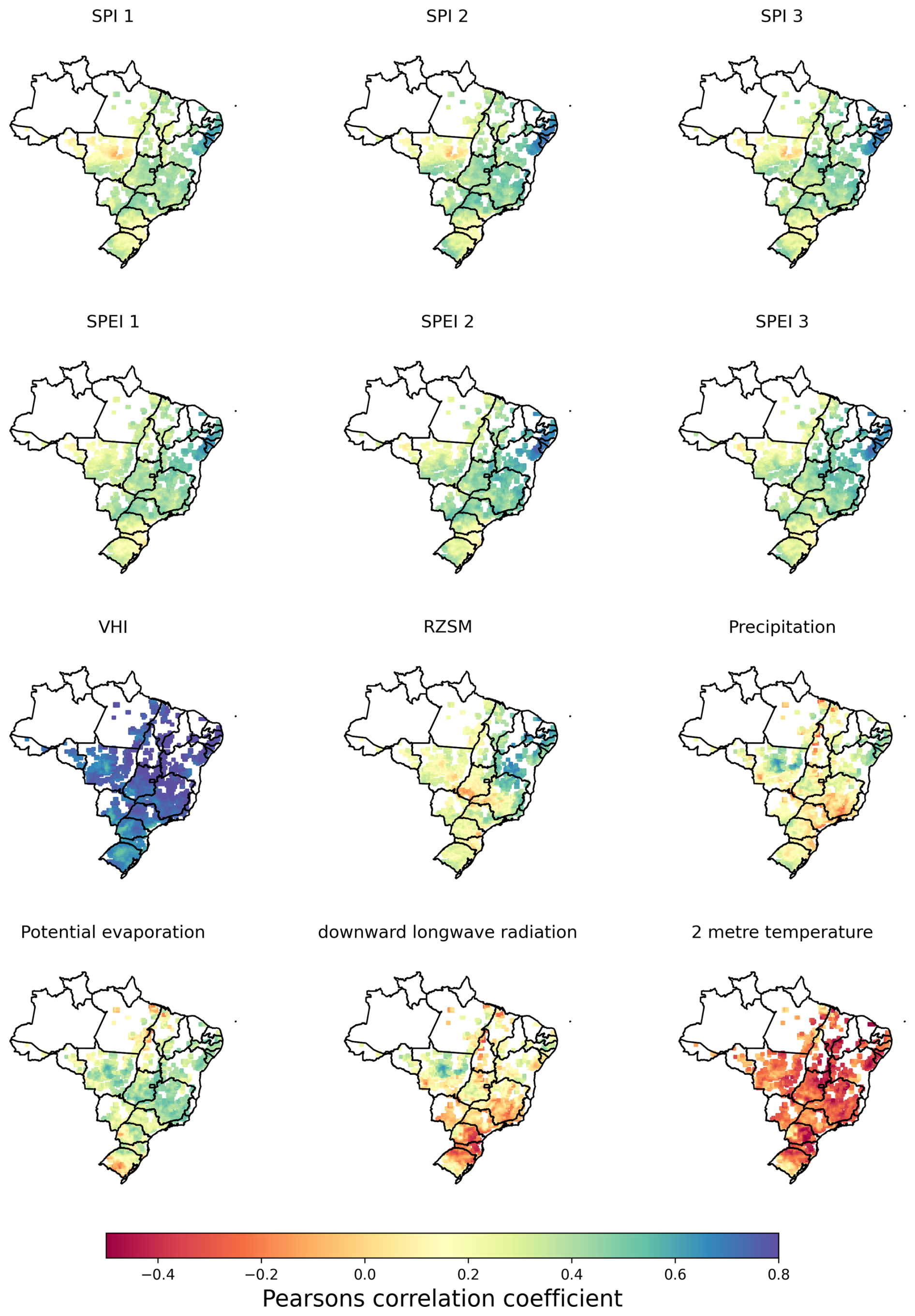
Figure 2 Correlation coefficient between the vegetation health index and input variables used in this study.​​​​​​​

Other variables included in the modelling process may also be significant drivers of the VHI. Figure 2 shows the correlations between next month's VHI and root zone soil moisture (RZSM), precipitation, potential evaporation, downward longwave radiation, 2 m temperature, and the VHI of the present month. As expected, the highest correlations are between the present and subsequent months' VHI. RZSM has high correlations in the northeast but very weak correlations around central Brazil. The 2 m temperature generally has greater correlations with next month's VHI than downward longwave radiation.

The correlations in Fig. 2 were used to inform 1-month forecasts of the VHI using a variety of machine learning methods presented in the subsequent section.

3.2 VHI forecasts

The initial selection of models described in Sect. 2.4 is compared here in Fig. 3. The gradient boosting model (GBM) was able to achieve greater performance across randomized test years than the other models. For this reason, the GBM was then chosen for further analysis including testing against later years. Variable importance is described in Sect. 3.5. SEA AV denotes a “seasonal average” benchmark, which is simply a model which predicts each month at each location as the historical average for the month, for the location to be predicted. All models outperform this low benchmark. This allows for the conclusion that all models obtain performance greater than that which can be inferred entirely from seasonal variability in the VHI.

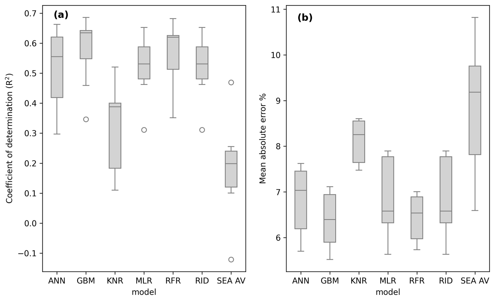
Figure 3 VHI forecasting model performance ((a) coefficient of determination, (b) mean absolute error) across a range of initially selected models. SEA AV refers to the monthly average model.

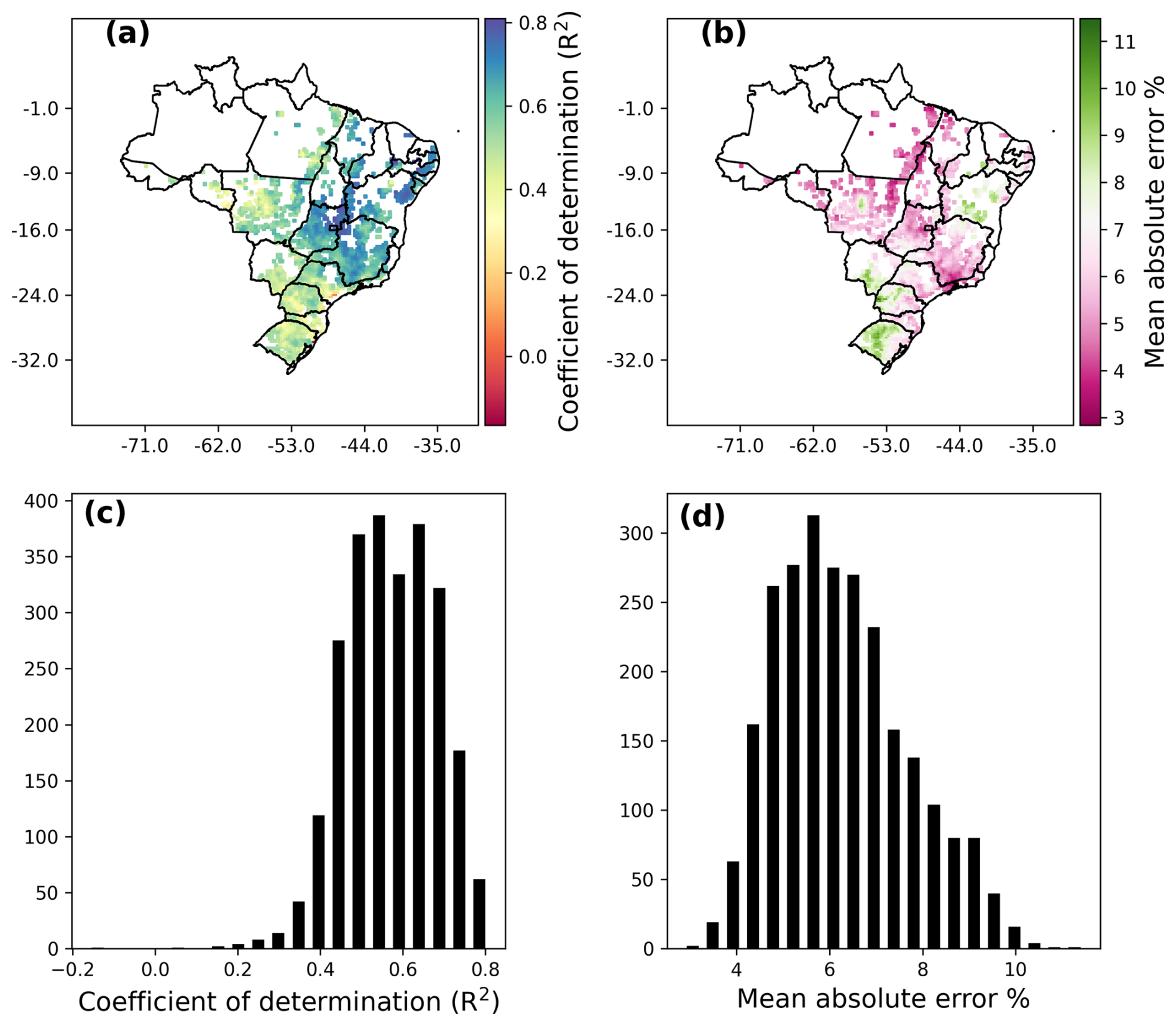
Figure 4 VHI forecasting model performance for the best model (GBM) across the spatial domain in Brazil, showing the R² score and mean absolute error for each grid cell location. Panels (a) and (b) show the spatial distribution of model performance for the two metrics; panels (c) and (d) show histograms of model performance metrics.

The best model from the initial comparison (GBM model) was taken and further assessed across the spatial domain (Fig. 4) and for the mode of the Southern Oscillation Index (SOI) (Fig. 5). Model performance in terms of R² is greatest in the east; some of the weakest correlations are in the west of the country and in the south and central regions. Figure 4c shows that generally R² values are between 0.6 and 0.75 for the gradient boosting machine learning method across grid cells. The distribution of mean absolute error values is less skewed, with most falling between 5 %–6 %.

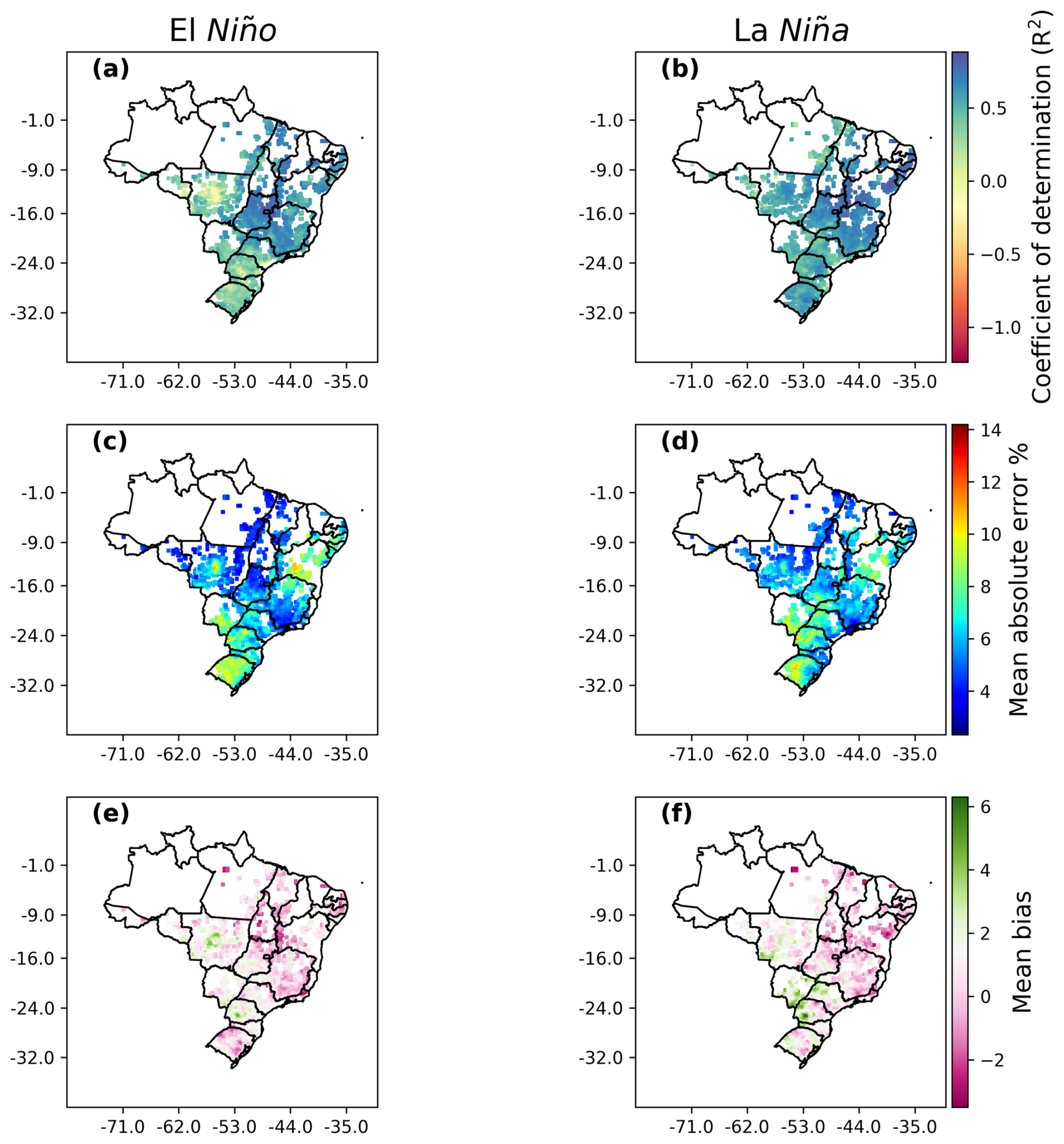
Figure 5 VHI forecasting model performance against positive and negative modes of the Southern Oscillation Index: negative SOI is associated with El Niño, and positive SOI is associated with La Niña weather events. Metrics are the coefficient of determination (a, b), mean absolute error (c, d), and mean bias (e, f).

3.3 Effects of the Southern Oscillation Index

Here, model performance metrics are split into El Niño and La Niña evaluation periods. Figure 5 shows how spatial trends in model performance can be affected by ENSO. For El Niño periods, model R² significantly reduces for central Mato Grosso, and there is a broader trend of decreases in model R² values across the south. This trend is also shown for mean absolute error. Generally, La Niña periods are forecast better than El Niño periods.

Figure 5 also shows how the effects of ENSO can lead to either under- or overprediction of the VHI depending on the location and ENSO mode. Of note is the overprediction of the VHI in central Mato Grosso in El Niño periods and underprediction in the south. Generally, model performance is less affected by La Niña than El Niño.

3.4 Predicting onset of drought impacts on the VHI

It is also important for models to be able to forecast when drought impact may reduce the VHI below the alert threshold of 40 %. The metrics described in Sect. 2.6 are used here to determine the performance of the best model for forecasting if the VHI falls below 40 % in the following month. Typically, model precision is greater than recall, meaning that there is a bias towards overprediction of values above 40 % rather than overprediction of values below 40 %. This is to be expected, given the distribution of VHI values results in more values above 40 %.

Figure 6 shows overall recall and precision (Fig. 6a) and when separated by El Niño (Fig. 6a) and La Niña (Fig. 6b) weather events. El Niño affects model performance by increasing the range of precision and recall values, increasing the number of those values at the low end of the distribution.

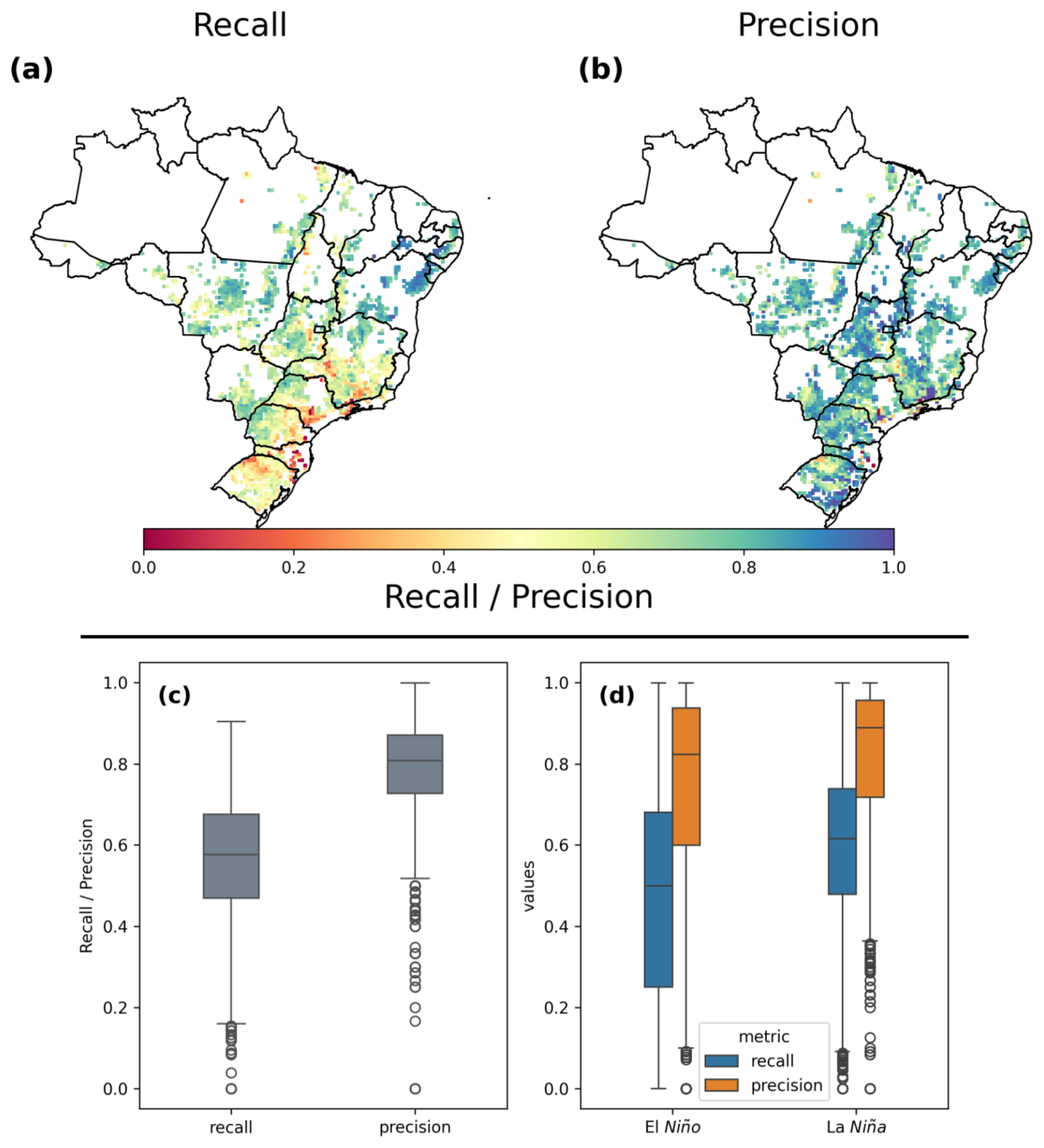
Figure 6 Recall and precision metrics shown both spatially (a, b) and as box plots (c, d). Panel (d) also shows the effects of ENSO on recall and precision.

Figure 6 also shows the spatial pattern of recall and precision (Fig. 6a and b​​​​​​​). Generally, recall is lower than precision, although there is no clear spatial trend in which regions may have higher or lower recall or precision. Lowest recall tends to be in coastal areas.

3.5 Variable importance

Correlations are measured between the strength of correlation between input and output variables and their correlation with model performance. This is shown for the SPI and the SPEI in Fig. 7 and for temperature and the VHI in Fig. 8. Here, we show the relationship between the strength of correlation between input variables and observed VHI and model performance measured by the coefficient of determination.

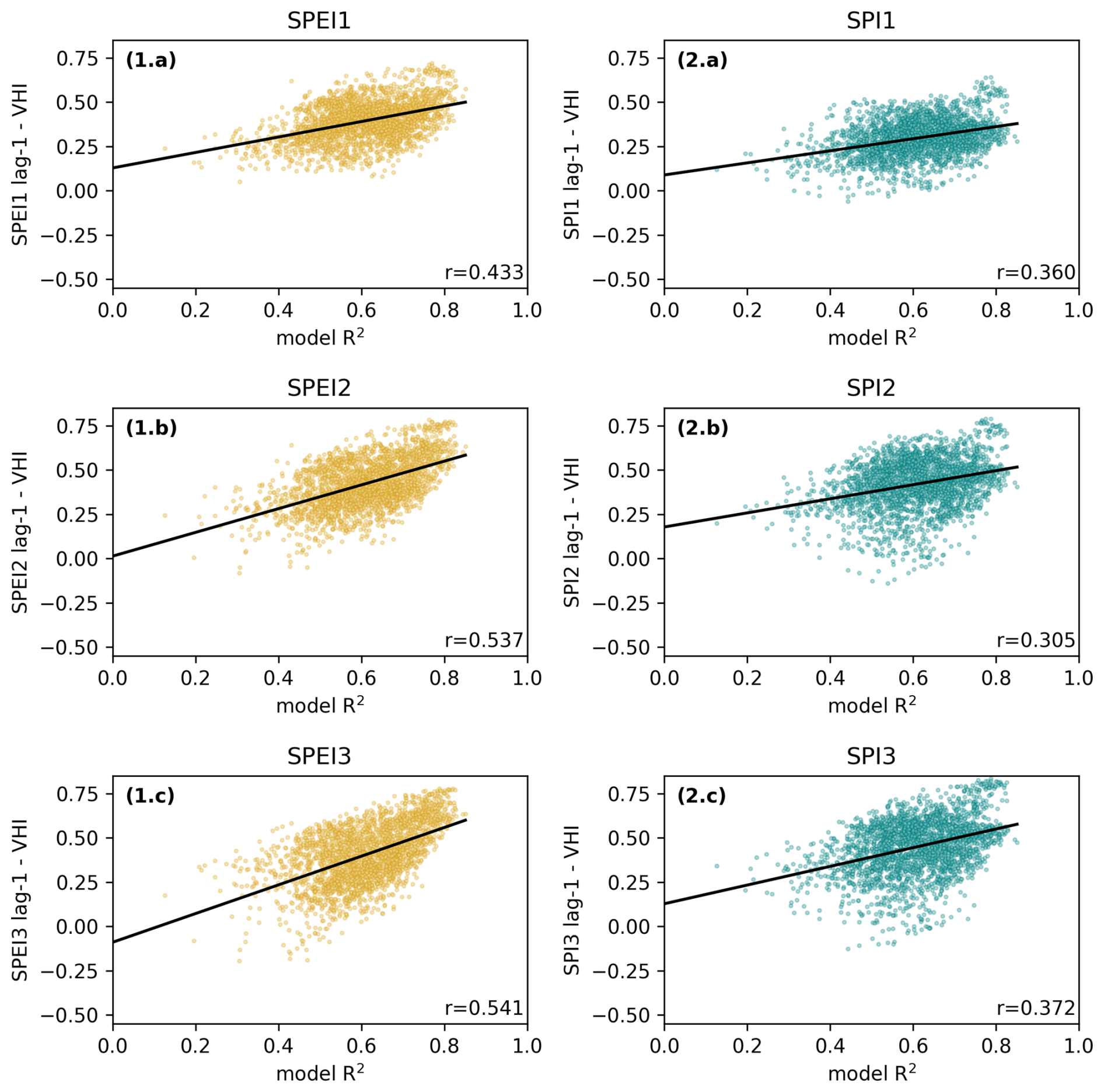
Figure 7 Pearson correlation coefficient between indices SPEI1–3 and VHI as well as between the SPI (1–3) and the VHI against model prediction performance measured by the coefficient of determination (R²). A line of best fit is plotted in blue for each panel with the R value on the bottom right. Each point represents the modelled R² at a single grid cell with corresponding SPEI–VHI and SPI–VHI relationships.

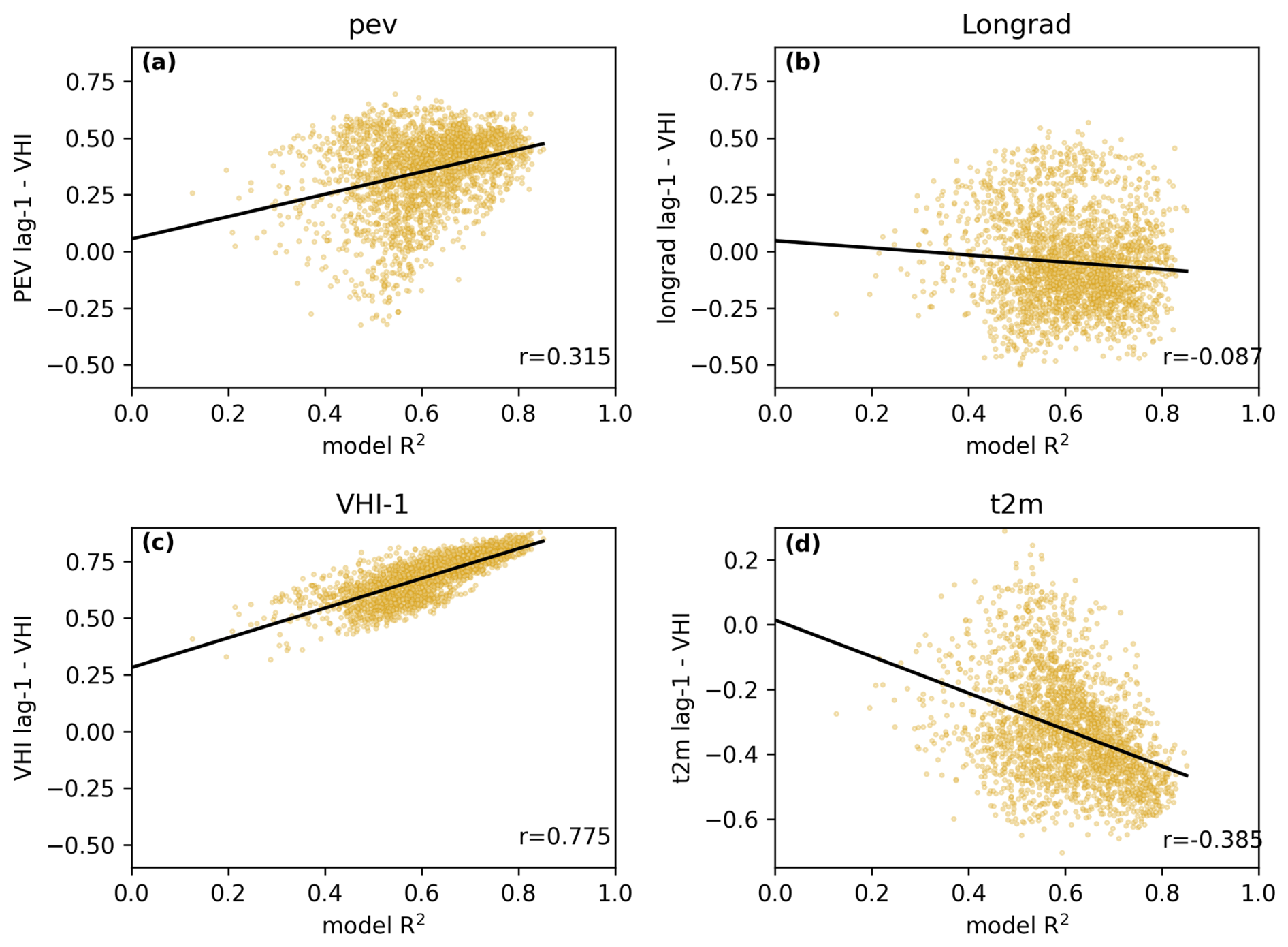
Figure 8 Pearson correlation coefficient between temperature effects and the VHI against model prediction performance measured by coefficient of determination (R²) as well as VHI autocorrelation. A line of best fit is plotted in blue for each panel with the R value on the bottom right. Each point represents the modelled R² at a single grid cell with the corresponding variable and VHI relationship.

Figure 7 shows that model performance is more highly correlated with longer accumulation periods of the SPI and the SPEI. Furthermore, the SPEI likely has a greater effect on model performance than the SPI. Figure 8 indicates that 2 m temperature may be a stronger variable to use to capture the effects of temperature on the VHI than other similar but correlated variables such as incoming longwave radiation and potential evaporation.

Spearman rank correlations between input variables are found in Sect. C. This was determined to show how correlations may affect variable importance and the highest correlating variables with the VHI.

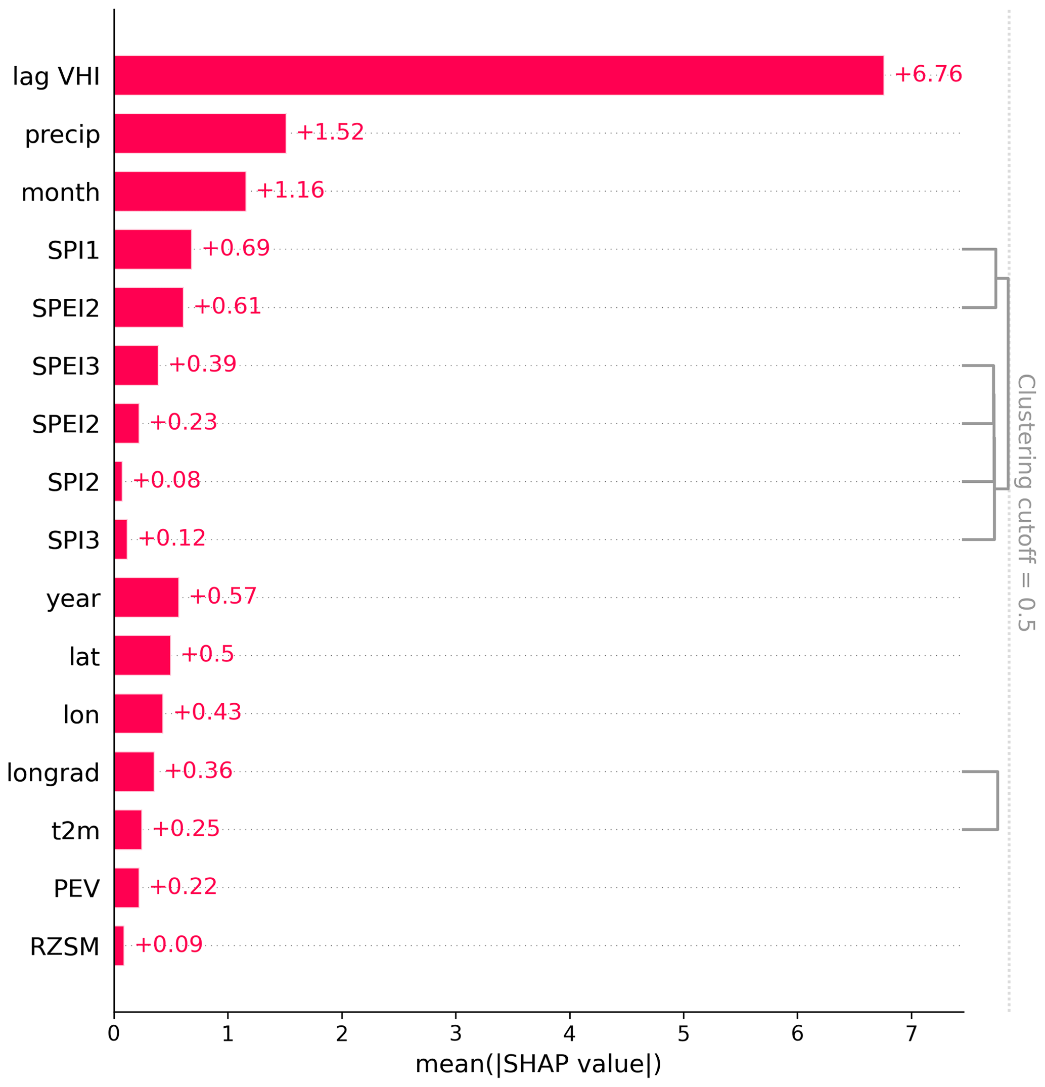
Furthermore, Shapley values were obtained for the gradient boosting method used in this study. Figure 9 displays Shapley values obtained. Shapley values correspond to the estimated relative contribution of each variable to model predictions (Molnar, 2022). Values indicate, similarly to the above analysis, that the VHI obtained for the previous month is a strong contributor in the determination of the VHI for the next month. The month variable is likely also highly influential as it is used as a proxy for seasonality. Other variables which are highly correlated (such as SPEI2 and SPEI3) may have lower contributions due to correlations between variables.

Figure 9 Shapley values obtained for each of the model input variables.

4 Discussion

Model performance varies upon the relationship between soil moisture, the SPEI, the SPI, and the VHI across Brazil, as well as the temporal autocorrelation of the VHI. The VHI in south Brazil (where rainfall is generally higher) is generally more difficult to forecast. For this reason, forecasting models presented here are most appropriate to be used in primarily moisture-driven regions (with most useful results for the northeast). The results presented here are of great significance for drought monitoring and forecasting efforts in Brazil and for others who may use studies such as this to inform other drought monitoring and forecasting work for other countries and regions. Here, we show that machine learning is capable of accurately forecasting the spatio-temporal variability in the VHI across Brazil and can also determine when VHI values are likely to fall below the 40 % drought stress threshold. Gradient boosting methods are an excellent method to use for both these evaluation metrics. Model performance is affected by El Niño events in the south and central Mato Grosso. Although machine learning is able to forecast when the VHI falls below 40 %, typically model precision is greater than recall. This means that the model is more biased towards forecasting VHI values above 40 %, which is as expected given the distribution of VHI values.

4.1 Regional variability in VHI

Vegetation health index variability is greatest in the northeast semi-arid region of Brazil. In this region, the VHI is more greatly driven by rainfall and subsequent moisture effects than any other region in Brazil. This makes the northeast the most easily forecast region. In the south and Central West regions (particularly Mato Grosso State), this trend results in poorer model performance in these regions. Subsequently, temperature effects are greater drivers of the VHI in these regions. This is likely due to the regional effects of limiting factors, which limit the growth of crops and vegetation and are known to vary spatially with varying climate (Sacks et al., 2010).

4.2 Spatial heterogeneity and temporal autocorrelations

Temporal autocorrelations across space indicate high monthly autocorrelation for the VHI. These temporal autocorrelations help to improve the ability to forecast the VHI on monthly timescales. The VHI temporal autocorrelation is highest in the northeast. This is a decisive factor contributing to greater model performance in this region.

4.3 How to build the most useful model for subseasonal VHI forecasting in Brazil

The results presented here provide key insights into the development of machine learning methods to forecast the effects of drought on vegetation health. Recommendations for how to build a forecasting model come in the form of two key factors: machine learning architectures and indices. Accurate forecasting requires a method of appropriate complexity. The appropriate level of complexity should strike a balance between model explanatory power and number of parameters to constrain. This study clearly indicates that linear methods such as multiple linear regression lack the explanatory power to effectively forecast forthcoming drought impacts and trends in the VHI. Conversely, some methods may be too complex; in this circumstance, gradient boosting methods outperformed the artificial neural network. Neural networks contain a large number of parameters, which ultimately require more data to be adequately constrained. This can cause model training to be a far greater challenge.

The choice of climate indices and variables is also a key question when building a forecasting model. In Brazil, the wide range of biomes across the country can mean that the influence of certain indices such as the SPEI and the SPI may be of greater importance in some regions than in others. Particularly, dry areas in the northeast are more affected by the drought-based indicators SPEI, SPI, and RZSM. Furthermore, although the SPEI may be more influential than the SPI, it is more important that longer-term indicators of 3 months are used above shorter 1-month accumulation periods. Of course, using the temporal autocorrelation in the VHI is a key factor in determining model performance. Regions which have the greatest monthly VHI autocorrelation also are the most easily forecast. Temperature variables are more useful for the forecasting of the VHI in south Brazil, where typically rainfall is higher and drought is less common in occurrence.

Here, models were trained for VHI value forecasting, and then the ability of the best model to determine onset of drought is found in Sect. 3.4. This resulted in high precision with slightly lower recall, meaning that model bias is towards forecasting values of the VHI above the 40 % threshold. For the forecasting of drought onsets, a more effective method to train models may be to use a classification model with altered training data to oversample VHI instances in which the VHI is below 40 %. There are many methods which can be used to improve dataset balance and improve recall, such as ensemble-based methods, over- and undersampling strategies, and synthetic minority oversampling methods (Chawla, 2010). However, in doing this, forecasting of VHI values would require a separate model.

4.4 Scope of methods analysed

Here, we analyse machine learning methods including artificial neural networks, gradient boosting and random forest methods, nearest neighbour methods, and linear regression methods. Among the methods excluded are convolutional LSTM models as discussed by Kladny et al. (2024) as well as other deep learning methods such as an ensemble of temporal convolutional neural networks (Miller et al., 2023). These model frameworks were excluded from the methodology following the general principal of Occam's razor to evaluate simpler methods first before expanding the scope of the work to more complex methods with greater numbers of parameters given time constraints. Evaluating such methods in the region should be a priority for future work building from this study.

In this study, machine learning methods are trained and evaluated on both maize and soybean growing areas together. Results for models trained on maize and soybean growing areas separately are presented in Appendix D. This analysis indicated that the differences between the performance of models trained on maize and soybean growing areas separately would not be significant. A likely contributing factor to this is that there is much overlap between maize and soybean growing areas (see Fig. 1), particularly because maize is often grown in rotation with soybean (dos Santos Canalli et al., 2020; Carvalho et al., 2014).

4.5 Comparison with other forecasting studies

Although this is the first study to forecast drought stress using the VHI across Brazil, this work fits into a broader context of other studies which address drought monitoring with vegetation indices. A major separation of this work from many other studies is the timescales involved. To the authors' knowledge, there were few studies at the time of writing that forecast the vegetation health index as far in advance as 1 month. One study (Lees et al., 2022) used a variety of neural networks to forecast the monthly VCI in Kenya and achieved very strong performance metrics. By contrast, Nay et al. (2018) forecasted an EVI for 16 d intervals using gradient boosting methods. Correlations between predictions and observed data varied between around 0.75 and 0.8 for agricultural land in two different regions. Given the longer lag time for our study, it would be expected that correlations may be lower (given that autocorrelations may decrease over time). Some other tools have been applied to forecast vegetation indices in dry climates such as in Tadesse et al. (2014), who used a statistical method known as VegOut to forecast the SDNDVI (the NDVI normalized for the historic record). Coefficient of determination values varied between 0.72 and 0.9 depending on the month evaluated (between June, July, and August) for 1-month forecasts for the region tested. Across studies found in the literature, results indicate that machine learning methods can be highly useful for forecasting vegetation health to assess drought stress, even at longer timescales such as per month (Kladny et al., 2024; Nay et al., 2018; Tadesse et al., 2014; Lees et al., 2022; Adede et al., 2019; Hammad and Falchetta, 2022). Such conclusions agree with the results of this study.

4.6 Future model developments for Brazil drought monitoring

To expand on the scope of this study, further work should focus on the application and assessment of machine learning architectures such as those described in Sect. (4.4). Such methods have been shown to improve vegetation health forecasts in other regions (Kladny et al., 2024; Miller et al., 2023) and so may also improve results here. Furthermore, improvements could be made to the forecasts of specific months key for agricultural production. Here, the best model trained can have variable performance depending on the month of assessment. A greater assessment of sampling methods or the targeted use of model ensembles may improve the stability of model performance for key months. For many regions November–March of the next year can encompass a typical growing season (CONAB, 2022). Therefore, these months are of greater importance.

This work aims to inform future developments in drought monitoring for Brazilian agriculture at CEMADEN. Forecasting the VHI would help to identify areas potentially affected by drought 1 month in the future. Currently, forecasting of next month's SPI is used to measure the potential impacts of drought, since rainfall anomalies are critical as a hazard. The forecast of the VHI can provide information on potential impacts, since it reflects on the vegetation health. This information is essential for disaster preparedness and planning of future actions to support areas affected by drought. The identification of drought evolution can inform decision makers in several agencies and levels of government on how to manage resources destined to alleviate drought impacts on agricultural activities.

5 Conclusions

This study addresses several questions important for building an agricultural drought forecasting framework for Brazil. In summary, the key conclusions of this work are as follows. Machine learning methods have great potential to be used to forecast agricultural drought 1 month in advance, and gradient boosting methods are able to achieve a coefficient of determination of up to ∼ 0.8 in some areas such as the northeast, making them an especially promising method to use. This work also shows that for some regions across Brazil the SPEI may be a more useful indicator than the SPI alone. For the agricultural drought onset forecasts, models also performed well, but further work is needed to test different methods of classification. ENSO variation had small effects on model performance, with El Niño effects being more difficult to predict than La Niña effects.

These findings are of significance for future drought monitoring and forecasting work in Brazil as well as for other regions in which drought monitoring and forecasting systems using machine learning are being considered or developed. Specifically, in showing how machine learning methods perform across Brazil, this research provides a first benchmark set of results for agricultural drought forecasts in the country. This also provides useful information about the spatio-temporal pattern of model performance. For future research outside of Brazil, this work provides a case study as to how machine learning methods perform across a wide area with a large diversity in climate.

Future work should aim to build upon these results to further aid drought monitoring efforts with improvements to model performance through additional pre-processing techniques and further assessment of machine learning modelling frameworks.

Appendix A

Here, we show results from the optimization of certain hyperparameters for the models investigated in this work. Hyperparameters are global parameters which affect the learning process rather than the model itself. Hyperparameters can include the learning rate of a neural network, the number of neighbours to use in the k-nearest neighbours algorithm, or the number of decision tree estimators present within a random forest model or gradient boosting machine. We undertook minimal hyperparameter optimization. We use the coefficient of determination to optimize hyperparameters across cross-validation folds. For gradient boosting and random forest models, we optimize the number of estimators which comprise the model. We found that above a certain threshold value (typically 2–10) the number of estimators which achieved the best results can vary if repeating optimization. For the k-nearest neighbours algorithm, the number of neighbours was varied between 5 and 1000, and 500 neighbours was found as the optimum value. For ridge regression, the regularization parameter (α) was optimized; however, results did not improve above those of the default value (1). The neural network was optimized by varying the number of neurons in each hidden layer and the number of epochs, which is the number of iterations through the dataset when training. Through optimization we determined 30 epochs with 25 neurons in each layer. We kept the number of hidden layers as small as possible (one layer) to avoid overparameterization. Model results with these optimized parameters can be found in Fig. A1.

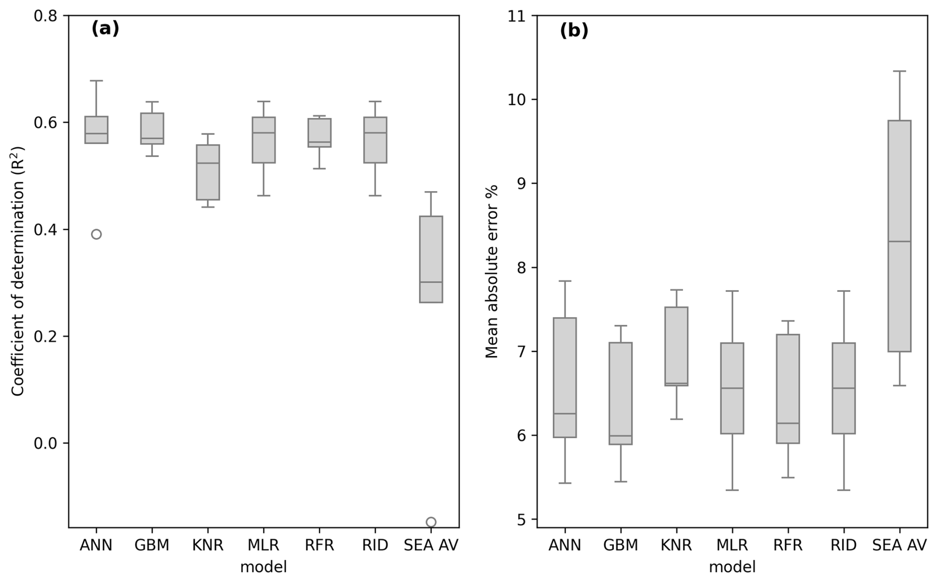
Figure A1 VHI forecasting model performance across the hold-out evaluation dataset for each of the initially selected models. Results shown are for optimized hyperparameters.

Some models achieved slightly better performance with optimization such as KNR. However, more data generally resulted in better model performance rather than optimized hyperparameters. Gradient boosting (GBM) is the best-performing model regardless of hyperparameter optimization.

Appendix B

Across months, VHI forecasts show little difference in the distribution of mean absolute error (Fig. B1). However, coefficient of determination values can differ much more between months. Figure B1a shows that January, February, September, and October are typically the most difficult months to predict. Because R² differs more than mean absolute error, this indicates that variability is more poorly captured in these months rather than there being a particular overall bias relating to the mischaracterization of the seasonal cycle of the VHI.

Further subsequent months after 1 month into the future were assessed to determine how model performance reduces for increased lag times. Figure B1 shows how model coefficient of determination reduces from a median of 0.69 to 0.35 and then to 0.16 when increasing the forecast lag time from 1 to 2 and then to 3 months.

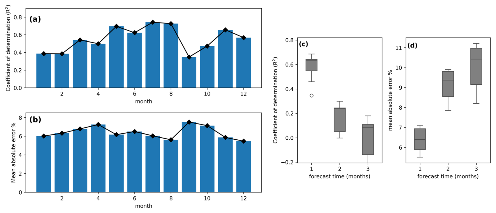
Figure B1 VHI forecasting model performance for the best model summarized as an average for each month, showing the R² score and mean absolute error per month (a, b). Secondly, model performance was compared for forecasts 2 and 3 months in advance (c, d).

Appendix C

Figure C1 shows Spearman rank correlations between each of the input variables. Highest correlations between input variables are between SPEI2 and 3 and SPI2 and 3 respectively. Both have a Spearman rank correlation of above 0.8. Secondly, t2m and longrad (both defined in Table 1) are also highly correlated (0.79).

A further variable was also included in initial tests (and in Fig. C1), which was the Southern Oscillation Index (SOI). The SOI provides an indicator of the mode of the ENSO, which can show whether El Niño or La Niña conditions are likely to occur. The Southern Oscillation Index was however shown to provide little information gain and adversely affected model performance in some instances. Therefore, this index was not included in the model results presented in this paper.

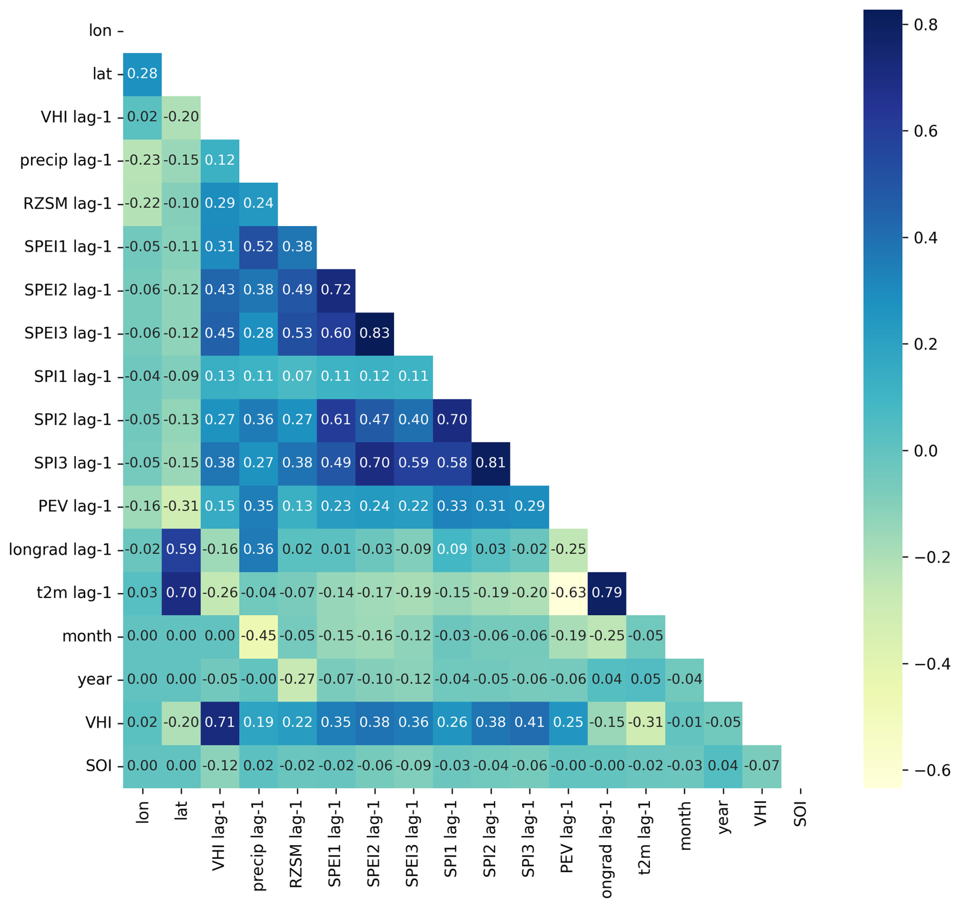
Figure C1 Spearman rank correlation between proposed input variables and the target variable (VHI), where lag-1 denotes a lag time of 1 month relative to the time step of the VHI.

Appendix D

In this study maize and soybean growing areas are combined to create a dataset used for training and testing the machine learning models. For contrast, Fig. D1 shows a comparison between model performance metrics of a random forest model if the model is trained using maize and soybean growing areas separately.

For the one model tested, there is little difference between training separately on maize and soybean harvested areas. This is likely because there is considerable overlap between the locations in which either crop is grown as they can often be grown in rotation (dos Santos Canalli et al., 2020; Carvalho et al., 2014).

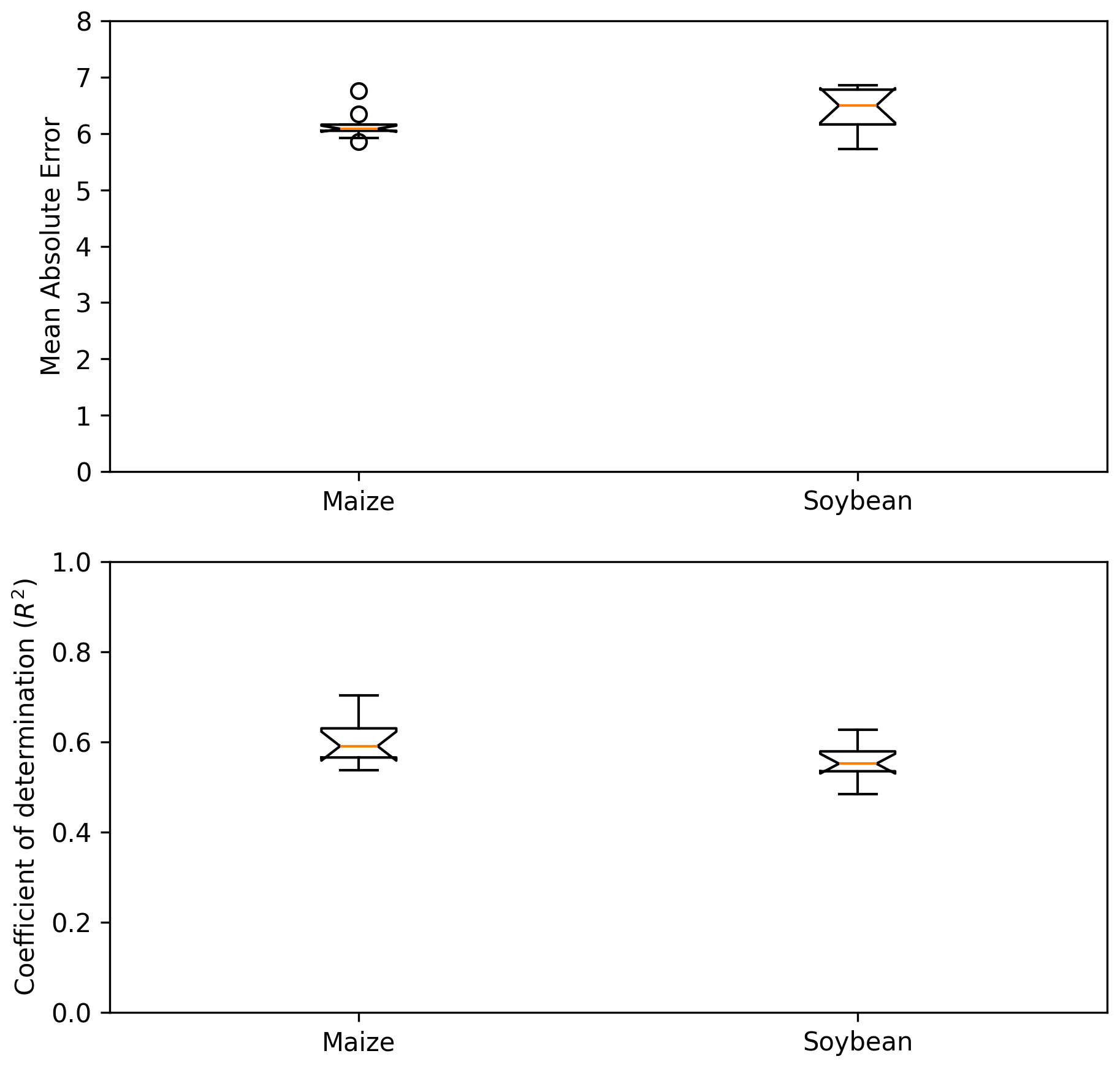
Figure D1 Mean absolute error (MAE) and coefficient of determination (R²) of a random forest model trained only using grid cells high in maize growing area and soybean growing area separately.

Appendix E

In this study, SPEI and SPI values are used for 1-, 2-, and 3-month accumulation periods. Periods longer than 3 months are not used for several reasons. Firstly, maize and soybean growth periods typically do not exceed 3 months, so using longer accumulation periods would not be indicative of crop growth (CONAB, 2022). Secondly, studies in the literature have shown that SPI1 to SPI3 better reflect agricultural drought development than longer accumulation periods such as SPI 6 and 12 (Łabędzki, 2007; Mohammed et al., 2022; Tanguy et al., 2023; Geng et al., 2016). Thirdly, a correlation analysis was performed between SPEI indicators and target VHI values for the following month shown in Fig. E1. This analysis shows that SPEI2 and 3 are more strongly correlated with the VHI than 6 and 12. For all of these reasons it was deemed that adding longer accumulation periods above the SPEI and SPI3 would not make a significant difference in forecast model performance.

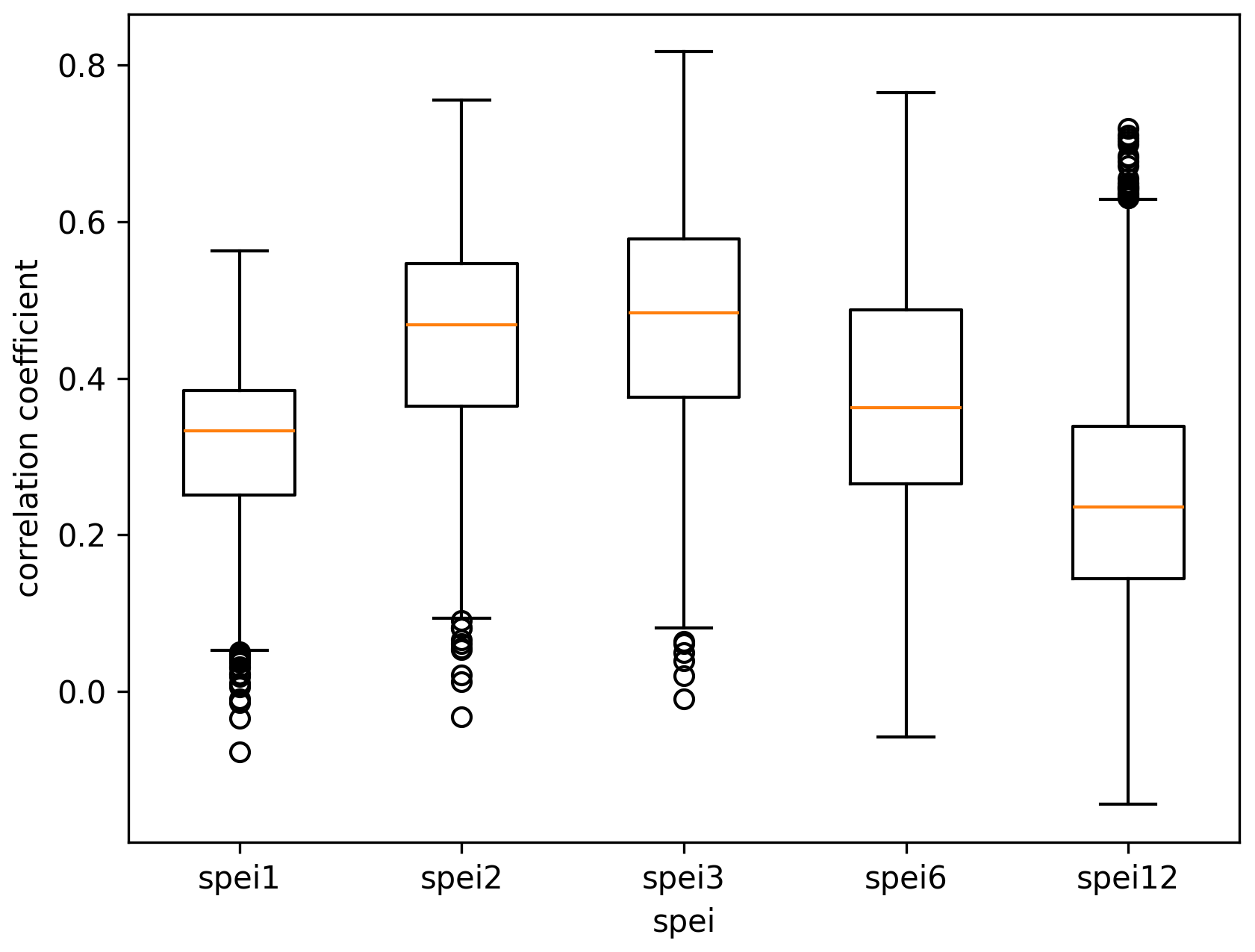
Figure E1 Correlation coefficient between SPEI indicators and observed VHI of the following month. Each correlation is calculated per grid cell (across 216 months) with box plots forming the spatial distribution of all correlations.