A data-driven framework for assessing climatic impact drivers in the context of food security

Understanding how physical climate-related hazards affect food production requires transforming climate data into relevant information for regional risk assessment. Data-driven methods can bridge this gap; however, more development must be done to create interpretable models, emphasizing regions lacking data availability. The main objective of this article was to evaluate the impact of climate risks on food security. We adopted the climatic impact driver (CID) approach proposed by Working Group I (WGI) in the Sixth Assessment Report (AR6) of the Intergovernmental Panel on Climate Change (IPCC). In this study, we applied the CID framework using a random forest model in a bootstrapping experiment to identify the most influential indices driving crop yield losses. We also used SHapley Additive exPlanations (SHAP) with the random forest model for explanatory analysis, enabling us to pinpoint critical thresholds for these indices–thresholds that, when exceeded, significantly increase the probability of impact. Additionally, we investigated the effects of two CID types (heat and cold and wet and dry) represented by categories of climate extreme indices on crop yields, with a particular focus on maize and soybeans in key agricultural municipalities in Brazil. We found that mean precipitation is a highly relevant CID. However, there is a window in which crops are more vulnerable to a precipitation deficit. In many regions of Brazil, for example, soybeans face an increased risk of yield losses when precipitation falls below 100 mm per month in December, January and February – marking the end of the growing season in those areas. Nevertheless, including climate means remains highly relevant and recommended for studying the impact of climate risk on agriculture. Our findings contribute to a growing body of knowledge critical for informed decision-making, policy development and adaptive strategies in response to climate change and its impact on agriculture.

1 Introduction

Climate extremes, such as heat waves, droughts, floods and excessive precipitation, play a critical role in determining crop yield shortfalls (Vogel et al., 2019). Empirical evidence from multiple studies shows that models incorporating data from several weather variables are more accurate in explaining crop production variability than those relying solely on precipitation (Proctor et al., 2022; Ray et al., 2015) or single weather variables. Consequently, it is essential to assess agricultural production risk through extreme climate indices, which are key to monitoring hazards that impact food production and food security (Das et al., 2022; Schyns et al., 2015).

These natural hazards affecting society are often referred to as “impact drivers”. As Ruane et al. (2022) argues, understanding impact drivers requires knowledge of the vulnerability and exposure of specific sectors. Sectoral information helps determine the magnitude of a driver's effect, which can be either beneficial or detrimental to its activities. This requires a co-creation process that aims to contextualize climate information for decision-making. This concept is embodied in the climatic impact driver (CID) framework, introduced by Working Group I (WGI) of the Intergovernmental Panel on Climate Change (IPCC) in its Sixth Assessment Report (AR6). The CID framework is still in its early development stages and aligns with the United Nations Sendai Framework for Disaster Risk Reduction (UNISDR) 2015–2030 (UNDRR, 2025), following the UNISDR hazard list definitions. However, the CID framework goes further by recognizing climate change as a significant hazard, which is not included in the UNISDR hazard list.

The formal definition of CIDs encompasses the physical conditions of the climate, including means, extremes and events. The CID framework emphasizes two critical aspects of risk assessment: defining indices for climatic impact drivers and identifying thresholds for climatic impact drivers (Ruane et al., 2022). These aspects reinforce the need to develop numerically computable indices that utilize one or a combination of climate variables to quantify the intensity and frequency of a CID. When these indices surpass certain thresholds, the risk of losses and damage increases. Although many indices have been used in the literature and summarized by Ranasinghe et al. (2021) for their relevance to the agricultural sector, it remains necessary to tailor approaches based on regional characteristics that bridge global insights with local solutions.

One way to understand the impact of climate change on agricultural production is through machine learning (ML) algorithms. ML algorithms can improve our understanding of how climate affects crop yields (Sidhu et al., 2023). Drawing on statistical learning theory (Vapnik, 1999), these algorithms can generalize patterns and make predictions from the available data. Several authors have applied ML algorithms to predict crop yields (Vogel et al., 2019; Sidhu et al., 2023; Han et al., 2019; Schierhorn et al., 2021; Silva Fuzzo et al., 2020).

Decision tree algorithms, such as random forest (RF) models, have been particularly effective in understanding the impact of weather extremes on crop yield variability (Vogel et al., 2019; Jeong et al., 2016; Schierhorn et al., 2021). The RF model combines tree predictors that are recursively split and used for predictions (Breiman, 2001). It provides insights into the importance of each feature in the model's overall performance. Studies by Vogel et al. (2019) and Schierhorn et al. (2021) have used this approach to explore the influence of extreme temperature and precipitation on predictive RF models for soybeans and maize. Both studies found that mean climate variables during growing seasons are the most relevant features for predicting crop yields. However, extreme weather indices, particularly those related to droughts and temperature extremes, can explain 18 %–43 % of crop yield variability (Vogel et al., 2019).

Despite efforts to improve the performance and interpretability of ML models, previous studies have relied on a somewhat limited selection of indices. As a result, other factors influencing crop yield variability may remain hidden and the underlying mechanisms of crop yield losses due to weather extremes could be overlooked. A generalized framework for variable and feature selection has been developed to enhance ML model performance, provide faster models and improve understanding of the underlying processes that generated the data (Guyon and Elisseeff, 2003). The backward recursive feature elimination (RFE) method, presented by Svetnik et al. (2004), leverages the RF algorithm's ability to generate variable importance as a variable reduction wrapper algorithm. Its applicability has been demonstrated in various studies, including those focused on crop selection (Wang and Li, 2023) and hyperspectral imaging for monitoring pasture quality (Pullanagari et al., 2018).

Although eliminating redundant features and variables can enhance our understanding of data structure, the challenge of interpretability remains. We propose using the model-agnostic explanation method introduced by Lundberg and Lee (2017), known as SHAP (SHapley Additive exPlanations). There are promising studies applying SHAP to environmental data (Wikle et al., 2023; Viana et al., 2021), with implications for soil moisture and evapotranspiration determination. The use of post hoc explanation algorithms for crop yields has been explored by Mariadass et al. (2022). However, to our knowledge, this method has not been specifically applied to predicting the impacts of extreme weather on food production.

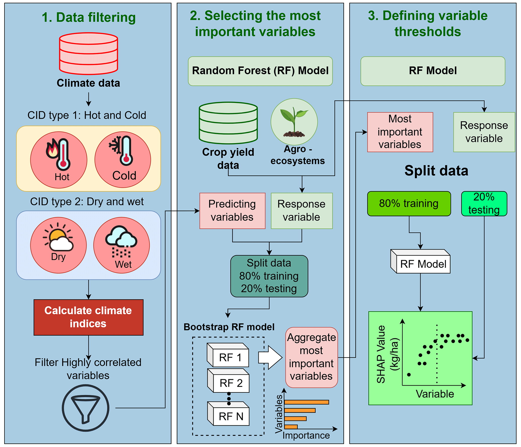
Figure 1 Flowchart illustrating the methodology proposed for analyzing the impact of climate indices on crop yield.

In this context, we introduce a comprehensive modeling framework to enhance the interpretability of tree-based models that utilize climate data to predict crop yield losses. With the goal of assessing the impact of climate extremes on food production, this research employs the CID framework developed by IPCC Working Group I (IPCC WGI). The framework allows us to characterize climate extremes by creating numerically computable indices and determining relevant thresholds. The significance of this framework lies in its ability to provide a basis for incorporating climate information into studies, decision-making processes and policy development. By applying this framework to our research, we aim to provide valuable insights that can inform critical decisions, policies and strategies related to food production in the face of climate extremes.

2 Methodology

2.1 Modeling framework

We present a framework for investigating the impacts of weather and climate extremes on crop yields using ML, focusing on building a reproducible workflow, selecting features and producing explainable ML model outputs. A good feature of an ML algorithm is its relevant nature in explaining the target variable (in this study, crop yields) based on input variables. However, it should not be redundant regarding any other relevant predictor (Yu and Liu, 2003). In addition to these concepts widely applied in ML methods, we add the concepts of explainable and operational features. In ML, a feature is any variable that is used as an input variable for prediction. Therefore, this work will use the terms feature and variable interchangeably.

This framework (Fig. 1) consists of three steps. The first is data filtering; in this step, we removed highly correlated features (Pearson correlation greater than 0.9). Feature selection is a preprocessing step in ML models. The filtering process removes redundant features. In this study, the concepts of explainable and operational features are the motivation for our proposed methodology. We aim to achieve a balance between model performance, interpretability and practical applications. By focusing on explainable features, our objective is to create models that offer clear insights into decision-making processes, thereby promoting transparency and reliability. This interpretability is essential for stakeholders who must comprehend and validate the model's results.

The second step aims to select the most important variables. We use the abilities of the RF to generate the importance of variables to rank the most important variables. The third step is to define variable thresholds. To do that, we must apply another machine learning model to explain the first one.

The SHapley Additive exPlanations (SHAP) explanatory analysis is an explanation algorithm proposed by Štrumbelj and Kononenko (2014) and uses game theory to provide an efficient explanation of the predictions made by a ML algorithm. The SHAP method is used to explain how each variable was used to make each prediction.

In the second step, we focus on identifying the most important CIDs to assess their impact on food production. Different models are independently trained for each state being analyzed; a separate and unique machine learning model is developed and trained using data specific to that state. This implies that the analysis of CIDs on food production is customized to account for the unique characteristics, data and conditions present in each state, rather than being applied a single model uniformly across all states. The feature importance determined based on entropy is determined by calculating the reduction in entropy (information gain) each feature provides when used to split the data at each node in the decision tree. Features that result in greater reductions in entropy across the tree are considered more important.

The creation of training, validation and testing subsets is crucial to avoiding overfitting and achieving reasonable estimates of model performance. The dataset was divided according to the chronological order of the data. The first 80 % of the data, according to the timeline, were used to train the model, allowing it to learn and adjust its parameters. The remaining 20 % were used for validation, meaning this portion was reserved for testing the model's predictions on data it had not seen during training. This approach, which incorporates a temporal aspect, is intended to simulate a real-world scenario where future data should be predicted. This method helps prevent overfitting by ensuring that the performance of the model is evaluated on new unseen data that come after the training period used, thus providing a realistic assessment of how the model will perform in practice.

To avoid temporal dependencies between data points from neighboring municipalities from being correlated within the same year, the best-fit model was selected using a leave-one-year-out cross-validation (LOYOCV) method and hyperparameters were chosen according to the mean CV performance in folds, following the recommendations of von Bloh et al. (2023). A fixed 10-year window was used for training, followed by 1 year as a test set. This process was repeated iteratively, leaving each year as the test set, while using the preceding 10 years for training. Performance metrics were calculated for each iteration, and scores were averaged to obtain an overall assessment of the performance of the model. The models were trained and optimized on the training dataset, and their performance was evaluated on the validation data to test the robustness of the models.

In the second step, we identify the most critical CIDs to assess their impact on food production. To achieve this, we used the RF model. Models were trained with three different crop yield datasets and different combinations of features, including precipitation means, temperature means, and combinations of means and extreme climate indices. The goal of this experiment was to identify the most important climate indices.

The third step builds on the results of the second step and uses the 10 most relevant climate indices employing RF explainability with the SHapley Additive exPlanations (SHAP) explanatory analysis. This approach aimed to provide a detailed understanding of how the model used these crucial indices and attempted to identify significant thresholds for these influential climate variables. The RF models were implemented using the R package ranger (Wright and Ziegler, 2017), and the SHAP results were implemented using the R package shapviz (Mayer, 2023).

The SHAP approach is based on explaining how each feature of the model was used to make a single prediction. The first step is to define a base prediction, which in this case is the expected value of the set X, which is the value of the adjusted and detrended crop yields E[f(X)]. Then, the RF algorithm is used to make a prediction f(x) for a single value of crop yield in a specific municipality and a particular year. The difference between the expected value and the prediction is called the SHAP value and preserves the unit of crop yields; therefore, here, it will be in metric tons per hectare.

In order to identify how each feature was used to generate the SHAP value, the algorithm recursively adds each feature and tests the importance of the feature for that prediction. However, the order in which the feature is added to the model is essential; that is why the principles of game theory introduced by Lloyd Stowell Shapley were used to solve the problem of allocating each feature's order and extracting its importance for the prediction. More details of the game theory used in SHAP results can be found in Strumbelj and Kononenko (2010).

The SHAP result was performed for each prediction using the R package treeshap (Komisarczyk et al., 2024). The package allows for generating a partial dependence plot, which is the relationship between the feature value and the contribution to the SHAP value. From this approach, we can find out which feature values are critical for crop yield losses, establish thresholds and contribute to the CID framework. Since the order of each feature is also evaluated, a second analysis is performed, which is used to evaluate the interaction between different features. In treeshap, the interaction between variables is determined by assessing the shared contribution of a pair of features to a model's prediction, beyond their separate effects. Initially, the SHAP values for each feature are computed to represent their individual impact on the model's output. For example, the interaction of features i and j is determined by subtracting the sum of their individual SHAP values from their combined contribution, i.e., $\text{interaction}={\text{SHAP}}_{i,j}-({\text{SHAP}}_i+{\text{SHAP}}_j)$. This method captures how the joint presence of two features affects the prediction compared to their independent contributions, uncovering synergistic or antagonistic interactions between the features.

2.2 Study area

Brazil is a significant producer of agricultural goods, as reported by the Food and Agriculture Organization (FAO) (FAO, 2025). The country is responsible for more than 10 % of the world's maize and more than 30 % of the global soybean production. Brazil is one of the four leading agricultural producers in the world, along with China, India and the United States, with a cultivated area of soybeans and maize of 58×10⁶ ha. In Fig. 2, we show the delimitation of the study area. The map shows 452 selected municipalities that encompass the states of Rio Grande do Sul (RS), Santa Catarina (SC), Paraná (PR), São Paulo (SP), Mato Grosso do Sul (MS) and Minas Gerais (MG). The selection criteria will be explained in the subsection “Crop yield data”. The map shows the percentage of cropland derived from the work of Potapov et al. (2022).

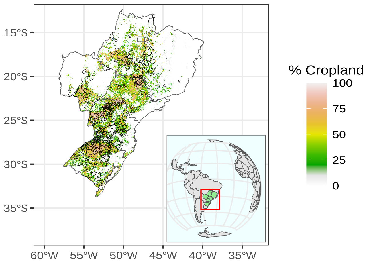
Figure 2 Location of selected study municipalities with respect to observed cropland extent between from 2003 to 2019.

The growing season in the study area was defined using a global crop calendar for the second season of soybeans and maize determined by data from Sacks et al. (2010). We consider the planting dates to follow a normal distribution, with the mean date being the most probable date for farmers and the maximum and minimum dates being considered to be twice the standard deviation. For soybeans, sowing dates start in the middle of austral spring in October, peak in November and end in December. The harvest begins in late summer and extends to fall, from February to March. Since the second season of maize peaks in February, we consider the end of soybeans to be in February. For the second season of maize, planting begins at the end of January, after soybean harvest; peaks in February; and ends in the beginning of April. The harvest starts in June, peaks in August and ends in October.

2.3 Data collection and processing

In this section, we present the description of datasets used to analyze the impact of climate variables on soybean and maize crops in the state of Paraná. We used two criteria to select a dataset: (i) the data must comply with FAIR principles (i.e., data must be findable, accessible, interoperable, and reusable), and (ii) climate data must be updated frequently (ideally, with a minimum of daily update frequency).

(IBGE, 2023)(IBGE, 2023)(Parana, 2021)(Iizumi and Sakai, 2020)(Muñoz-Sabater et al., 2021)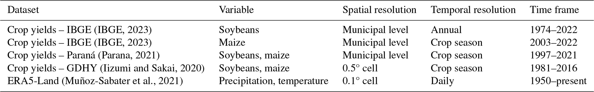

Table 1 Description of the datasets used in the case study.

We used three different datasets: (i) the statistical yearbooks of the state of Paraná (Parana, 2021), (ii) the Municipal Agricultural Production Survey by the Brazilian Institute of Geography and Statistics (IBGE) (de Geografia e Estatística, 2022) and (iii) the Global Dataset of Historical Yields (GDHY) (Iizumi and Sakai, 2020). For climate analysis, we used data from the fifth-generation European Centre for Medium-Range Weather Forecasts (ECMWF) ERA5-Land reanalysis dataset (Muñoz-Sabater et al., 2021). We summarized the main characteristics of each dataset used in Fig. 1.

2.3.1 Crop yield data

Crop yield data are a vital component in understanding the impacts of climate on food production. Crop yields are generally made available at the municipal level. We used three datasets to analyze crop yields in Brazil. We collected crop yield data from the Brazilian Institute of Geography and Statistics (IBGE) at the municipal level (de Geografia e Estatística, 2022). In the study area, the double-cropping system is widely adopted. It, therefore, represents a potential bottleneck because the IBGE data from 1974 to 2022 are an annual aggregation of the total production of that crop within the municipality.

However, the Brazilian Institute of Geography and Statistics has been collecting maize in the first and second season since 2003. This matches the period during which the second maize season intensifies in Brazil. Data at the municipal level were filtered based on data availability. The missing years were removed from the dataset, and the municipalities with more than 2 years of missing data were disregarded. The selection resulted in 452 municipalities for soybeans that comprise the states of Rio Grande do Sul (RS), Santa Catarina (SC), Paraná (PR), São Paulo (SP), Mato Grosso do Sul (MS), Minas Gerais (MG) and Goiás (GO) and 216 municipalities for maize in the second season for Paraná (PR), São Paulo (SP), Mato Grosso do Sul (MS), Minas Gerais (MG) and Goiás (GO).

The Department of Rural Economy (Departamento de Economia Rural, Deral) of the state of Paraná, Brazil, is also responsible for collecting crop data at the municipal level. The method of collecting and processing data is similar to what is done by the Brazilian Institute of Geography and Statistics; therefore, a high level of redundancy is expected from these two datasets. This redundancy is necessary to validate data and remove outliers that might reduce the quality of a model. The same number of municipalities selected using IBGE data was used in data from Deral.

The Global Dataset of Historical Yields is a global annual time series of 0.5° grid-cell estimates for maize, rice, wheat and soybeans from 1981 to 2016. For each grid cell, crop yields are estimated in t ha⁻¹ based on Food and Agriculture Organization (FAO) country-level yield statistics and then corrected using the remotely sensed leaf area index (LAI), the fraction of photosynthetically active radiation (FPAR) and crop-specific radiation use efficiency derived from reanalysis. Crop areas and crop calendars were derived from Sacks et al. (2010). More details about the dataset are described in Iizumi and Sakai (2020). The dataset was aggregated to the municipal level using zonal statistics in the terra package (Hijmans, 2023) in R Studio.

For statistical analysis, we removed the outliers of all crop yield datasets considering, for each year, neighboring municipalities using the interquartile range (IQR). For the outlier removal process, we defined “immediate regions” as clusters of municipalities geographically proximate to one another, as classified by the Brazilian Institute of Geography and Statistics. Crop yields within these regions exhibited a high degree of correlation, which was verified using the correlation index. To identify outliers, we applied the interquartile range (IQR) method for each year. Specifically, if the yield of a municipality in a given year deviated significantly from the yields of other municipalities in the same immediate region, it was classified as an outlier and excluded from the dataset. This approach ensured that only extreme and anomalous data points, not reflective of regional trends, were removed.

Changes in technology in seed production, fertilizers and land management, also known as technological trends (Liu and Ker, 2020), and other sources of trends such as climate change were removed by local polynomial regression fitting (LOESS) (Cleveland et al., 2017). Moreover, systematic changes in crop yields have also been associated with heteroskedasticity (Yang et al., 1992; Zhu et al., 2011; Ozaki et al., 2008). The residuals of the LOESS model were tested for heteroskedasticity. If heteroskedasticity was proved, it was removed using the method proposed by Ozaki et al. (2008). For further information on the preprocessing of crop yield data, please consult the Supplement.

2.3.2 ERA5-Land reanalysis dataset

Weather data were sourced from the fifth-generation European Centre for Medium-Range Weather Forecasts (ECMWF) ERA5-Land reanalysis dataset (Muñoz-Sabater et al., 2021; Hersbach et al., 2020). The dataset has a 0.1° × 0.1° latitude–longitude grid and was aggregated to the municipal area to match the spatial discretization of soybean crop yield (SBY). The data collection spanned 1980 to 2023, with daily observations. Weather variables included precipitation, maximum temperature and minimum temperature. We used different climate indices to evaluate multi-hazard risks. Since mean climate conditions of precipitation and temperature are the most relevant (Moriondo et al., 2011), we considered monthly precipitation, maximum and minimum temperatures, total precipitation, and mean temperature over growing seasons.

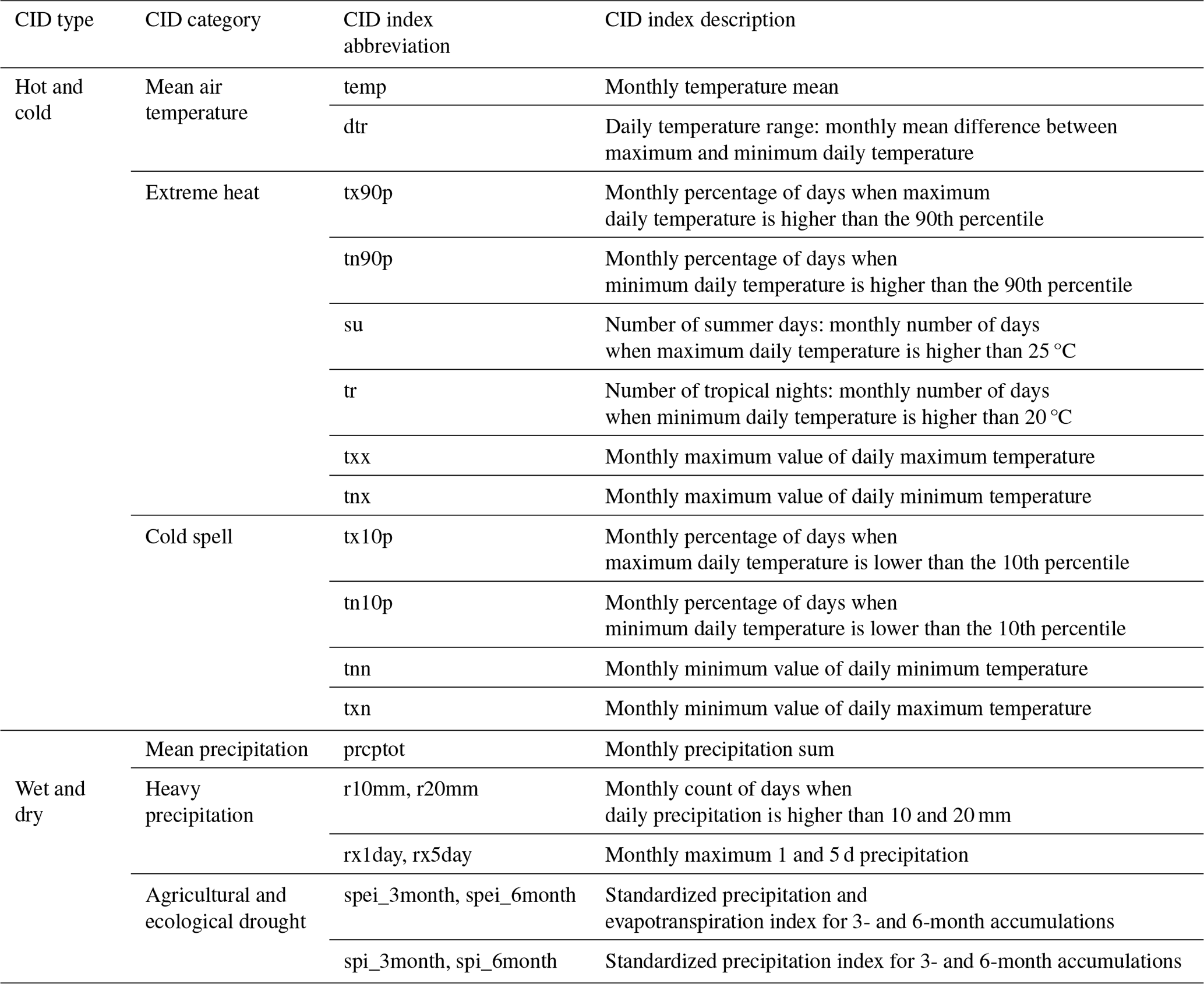
Table 2 Description of the climatic impact drivers (CIDs) considered in this study and their respective indices.

2.3.3 Indices for climatic impact drivers

The IPCC WGI has presented CIDs as a new approach to assessing climate data to analyze their effects on society. CIDs are represented by numerically computable indices and categorized into several types. In this paper, we considered wet and dry and hot and cold CIDs. To calculate the indices, we first considered the indices indicated by the Expert Team on Climate Change Detection and Indices (ETCCDI), which is supported by the World Meteorological Organization (WMO) Commission for Climatology, the Joint Commission for Oceanography and Marine Meteorology (JCOMM), and the research program on Climate Variability and Predictability (CLIVAR) Frich et al. (2002). A summary of the indices used according to the type of CID is shown in Table 2.

We also considered two drought-related indices, the Standardized Precipitation Index (SPI) (McKee et al., 1995) and the Standardized Precipitation and Evapotranspiration Index (SPEI) (Vicente-Serrano et al., 2010). The SPI is based on the probability of monthly precipitation on different timescales, and it is recommended to be calculated with a time series of at least 30 years. The monthly time series must be fitted to a cumulative distribution function (CDF). We adopted the gamma distribution.

Then, the data are transformed to the standard normal distribution to calculate the SPI, a standardized value subtracting the transformed precipitation from the mean value and dividing by the standard deviation. The SPI can be calculated using different timescales representing previous meteorological conditions, typically 1 to 48 months. For agricultural applications, the 3-month SPI is most frequently used Kim et al. (2019).

The SPEI is a more recent index that incorporates temperature in the calculation of the SPI. A new step was added to the procedure, calculating the monthly potential evapotranspiration (PET) and the SPI using the same procedure described previously with the value of monthly precipitation minus monthly PET. PET was calculated using the Hargreaves method, which is calculated using maximum and minimum temperature and extraterrestrial radiation (RA) (Droogers and Allen, 2002).

The primary motivation for using distinct indices derived from the same fundamental data is to identify which features of the extremes are the most significant. Is it the magnitude of an extreme, the length of time it lasts, or values that are either above or below a certain threshold? Research such as that by Vogel et al. (2019) has demonstrated the importance of extreme events in understanding the variability in crop yields. We summarize all the indices according to CID type and category in Table 2.

3 Results and discussion

The comparison of the datasets used in this study is important for evaluating the reliability of the data. High-quality crop yield data improve the calibration of crop growth models (Rosenzweig et al., 2014). However, they have a broader application in geosciences. Crop yield data are used to parameterize hydrological models in watersheds, especially in agricultural catchments, and improve soil moisture simulation (Sinnathamby et al., 2017).

We compared crop yields at the municipal level in Brazil. We observed that the IBGE and Paraná Deral data for soybeans and maize are highly correlated; however, outliers were detected in both datasets. The outlier removal process improved the agreement between the two datasets, suggesting that eliminating data improved the dataset's quality. Since Deral is only available in Paraná, for the other states of Brazil, the GDHY and IBGE data were compared. The Global Dataset of Historical Yields aggregated at the municipal level has a weak association with the other datasets. This result confirms what was reported by Iizumi and Sakai (2020). The GDHY data are based on satellite data collected from a fixed cropland map. In many regions of Brazil, there is a noticeable increase in croplands, which can influence the estimation of GDHY data. In addition, the exact location of the planted area within each municipality can vary from year to year.

Table 3 Correlation coefficients of three different crop yield datasets: (a) IBGE (n = 3845), Deral (n = 3120) and GDHY (n = 15 411) for maize and (b) IBGE (n = 20629), Deral (n = 3432) and GDHY (n = 15 406) for soybeans. Values represent the strength and direction of the relationships, with an asterisk (^∗) indicating statistically significant correlations of p < 0.001.

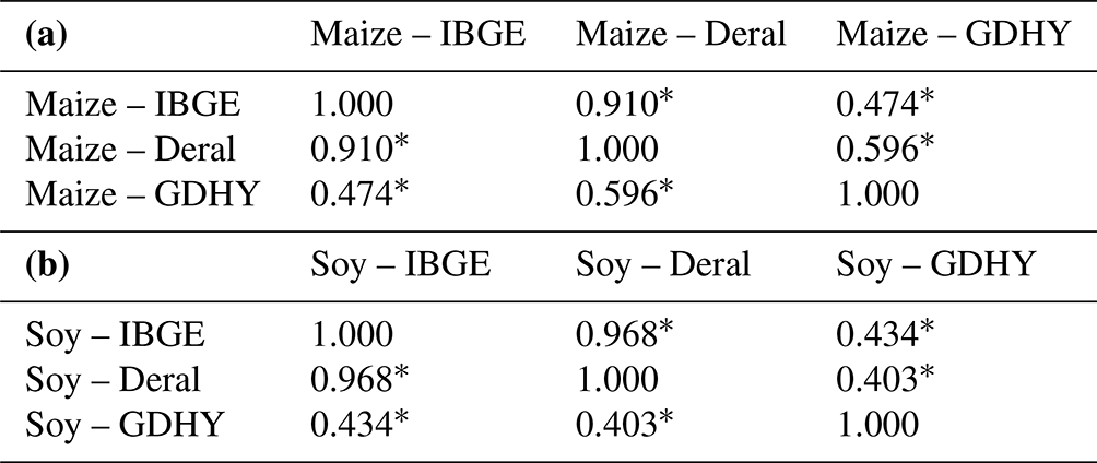
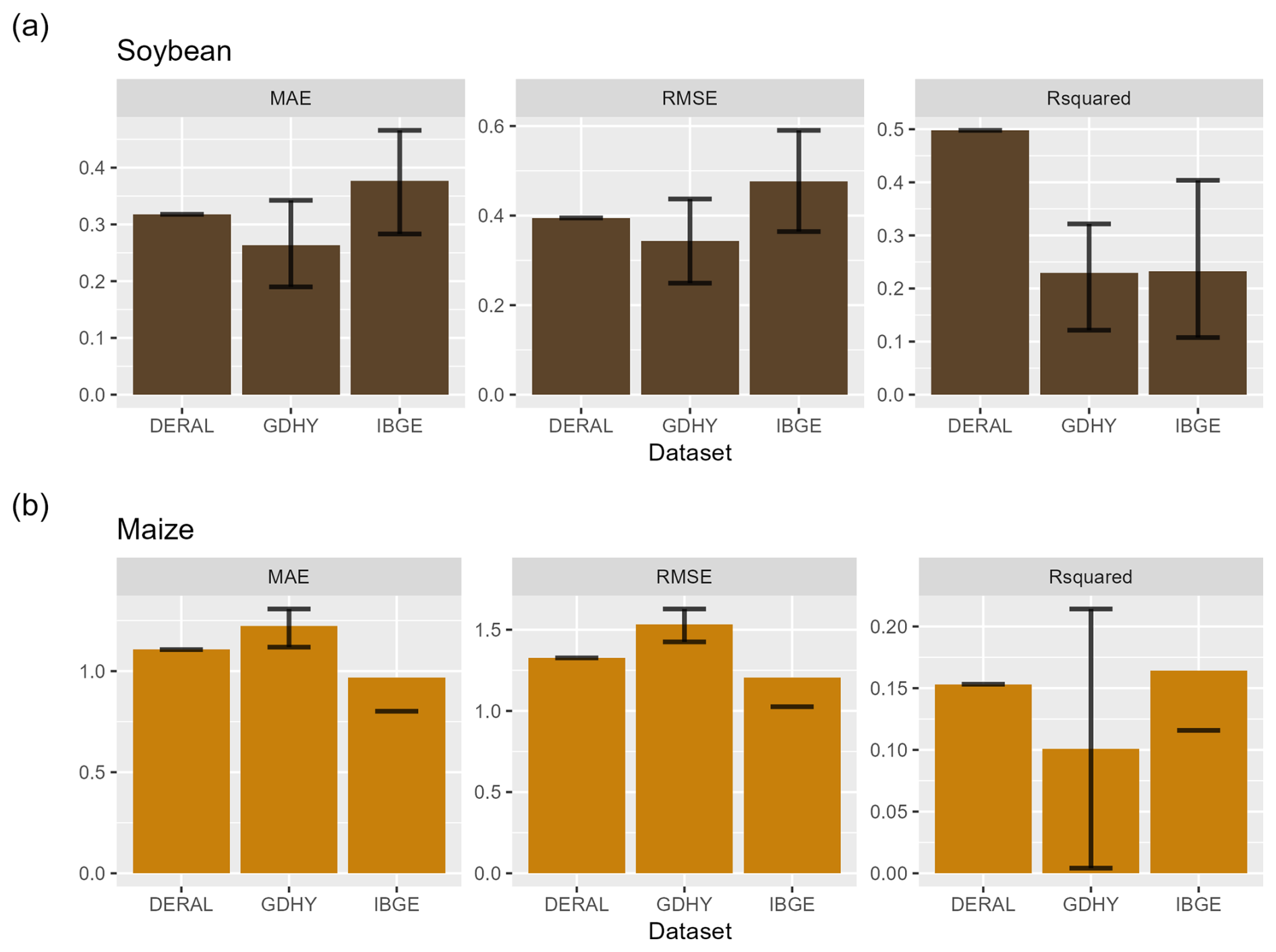
Figure 3 Performance evaluation of regression models for (a) soybeans and (b) maize. Data from the Department of Rural Economy (Deral) with data only for Paraná, Global Dataset of Historical Yields (GDHY), and Brazilian Institute of Geography and Statistics (IBGE) for major historically agricultural municipalities. MAE: mean absolute error, RMSE: root mean square error.

3.1 Identifying key climate impact drivers

We tested a variety of indices that measure mean precipitation, mean temperature and extremes. We initially tested the ML technique using various inputs to demonstrate its ability to illustrate crop yield variability in the states examined. In Fig. 3, we demonstrate the model performance of the RF model considering different datasets. Taking the coefficient of determination, the climate variables explained the variability in soybean crop yields, on average, from 30 % to 40 % for IBGE, 25 % to 45 % for GDHY and 30 % to 50 % for Deral. The climate was explained for maize from 12 % to 15 % for IBGE and Deral and from 10 % to 45 % for GDHY.

The coefficient of determination quantified the proportion of the variance in the crop yield data (dependent or target variable) that the RF model can explain. The results are consistent with the values found in other similar studies; Ray et al. (2015) used municipal-level data to quantify the impact of climate variability on yields using regression models and determined that, in Brazil, climate variability explains 26 %–34 % of soybean yields and 41 % of maize yields. Vogel et al. (2019) used the same dataset as Ray et al. (2015) considering South America and applied an RF model defining the values of 28 % for soybeans and 25 % for maize. It is important to note that none of these studies separated maize in the first and second season.

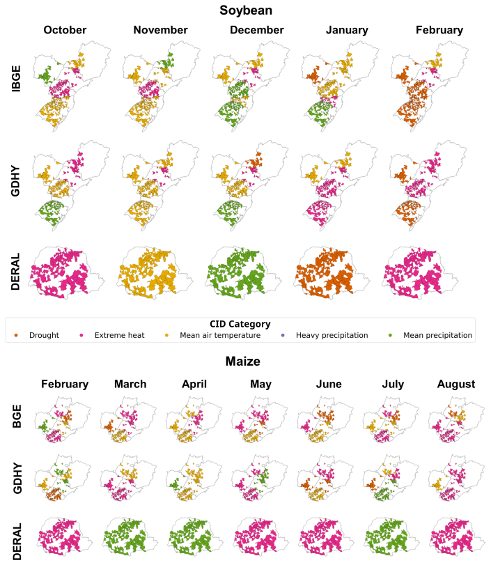
Figure 4 Importance of key CID categories in predicting soybean and maize crop yields. The figure displays the most significant features identified by the random forest model for soybeans and maize.

The model performance was generally higher for GDHY than for the other datasets for soybeans in the southern states (RS, SC and PR). The models based on precipitation means and the combination with temperature and extremes explain the variability in crop yield more than only the temperature means, which was observed in all three datasets. For maize in the second season, for MS, MG and GO, the models that combine mean temperature to mean precipitation and extremes explained the variability in crop yields more than only temperature, which was observed in GDHY and IBGE. The IBGE database showed that the maize model was much more effective in São Paulo than in any other state.

The RF models used in this study helped obtain the most relevant variables, and these variables were classified into CID types, i.e., wet and dry and hot and cold, and subcategories, as described in Table 2. The model demonstrates the importance of climate variables in explaining the variability in crop yields and allowed us to determine the critical CIDs considering each state and dataset. The following sections summarize the key CID categories for soybeans and maize.

Feature importance was summarized spatially and temporally. Figure 4 highlights similarities and dissimilarities regarding feature importance considering the different datasets.

In the Supplement, we show tables with the results of variable importance for all models. The analysis of variable importance for soybean datasets is shown in Table S1 in the Supplement. The analysis identifies extreme heat (tnx), the drought index (SPEI) and precipitation totals (prcptot) as key variables that affect crop yields in different regions. These climate factors are crucial for predicting agricultural outcomes, with extreme heat and drought having a great impact on the results. The significance of these variables varies by region; for example, extreme heat and drought are critical in Paraná during February, while mean air temperature and extreme cold in January matter more in Minas Gerais. February and January are highlighted as pivotal months due to their association with significant climate events. In general, the results highlight the importance of addressing both heat and water stress in agricultural systems while taking into account spatial and temporal differences to enhance predictive accuracy.

For maize in the second season, the results are shown in Table S2. For Paraná (PR), key variables are April precipitation and May heat, which influence agricultural outcomes. Goiás (GO) is significantly affected by the April diurnal temperature range and the heat and precipitation of May. In Minas Gerais (MG), May precipitation is crucial, with the March temperatures and August heat also significant.

Mato Grosso do Sul (MS) deals with February temperatures and June heat and drought. Rio Grande do Sul (RS) sees the diurnal temperature range of May as vital, along with the March drought and the July–August precipitation. São Paulo (SP) contends with the heat of August and the rainfall of July, emphasizing the importance of temperature and precipitation on environmental and agricultural concerns.

3.1.1 Wet and dry

Changes in mean precipitation pose a threat to agricultural production. A precipitation deficit leads to the reduced availability of soil moisture, affecting plant development and reducing crop yields, and it is considered the most critical environmental factor that reduces crop yields (Bray, 2007). In our analysis, mean precipitation was one of the most important climatic impact drivers of soybean crop yields during January and February for RS, SC, PR and MS and also in December for PR.

The state of Rio Grande do Sul has historically been affected by El Niño–Southern Oscillation (ENSO), with a more substantial influence from November to May (Gelcer et al., 2013), which is responsible for droughts and the impact on soybean crop yields during La Niña. The model did not indicate that mean precipitation was the most important factor for the state of SP. For maize production, mean precipitations during April and May were considered important for PR, MS, MG and GO and not for SP.

Agricultural systems require minimum rainfall, or they rely on irrigation. In Brazil, the states of SP, MS, MG and GO have a well-defined difference between wet and dry seasons. Usually, the wet season starts in October and ends in May, and the soybean–maize double-cropping system depends on the length of the wet season in the states mentioned above.

Agricultural and ecological drought indices are directly related to a precipitation deficit and excessive temperature (Sarhadi et al., 2018; Lesk et al., 2021), which affect the ability of plants to grow and reduce plant transpiration. The duration and timing of droughts play a significant role. We observed that droughts occurring in January and February during the rainy season were the most important for soybeans. The droughts in February and March also affected the second-season crop yields of maize. Droughts that occurred at the end of the maize growing season also affected crop yields.

In this study, we considered climate extreme indices on different timescales. As we added the temporal dimension to the analysis, we revealed that a 3-month SPEI in October in the state of RS was selected for the list of the most relevant variables. This indicates that pre-sowing meteorological factors that can reduce soil moisture conditions also influence crop yields. This result corroborates the findings of Santini et al. (2022), which revealed that a drought analysis should not neglect antecedent conditions since it influences factors such as soil workability and crop development.

3.1.2 Hot and cold

The mean air temperature influences many aspects of crop cultivation. In RS and SC, the soybean growing season starts when the mean temperatures exceed the minimum temperature thresholds for soybeans (Battisti and Sentelhas, 2014). As the temperature increases, the development (phenology) of the plant is affected and increased thermal stress is expected Lesk et al. (2021). Except for RS, mean temperatures during all soybean growing seasons were considered important variables. The same behavior was observed for maize; mean temperatures were considered significant during all growing seasons.

Exposure to temperatures above a specific limit or threshold can lead to lower yields. The value of these thresholds depends on the crop species and farm management. For soybeans, extreme temperature indices affected crop yields throughout the growing season, especially in January and February.

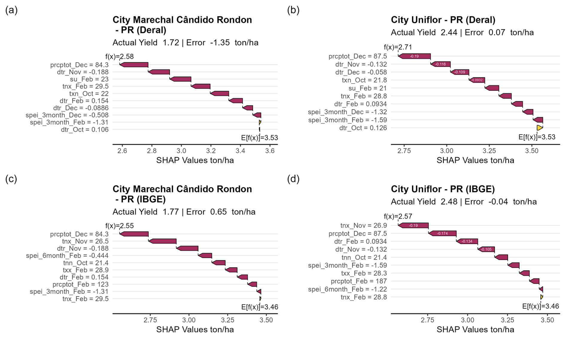
Figure 5 SHAP waterfall plot visualizing the key CID contributions to crop yield losses for the state of Paraná (PR) in 2019, a drought year, with metrics for monthly maximum value of daily minimum temperature (tnx), minimum value of daily maximum temperature (txn), minimum value of daily minimum temperature (tnn), maximum value of daily maximum temperature (txx), percentage of days when tx > 90th percentile, standardized precipitation evapotranspiration index (SPEI), total precipitation (prcptot) and daily temperature range (dtr).

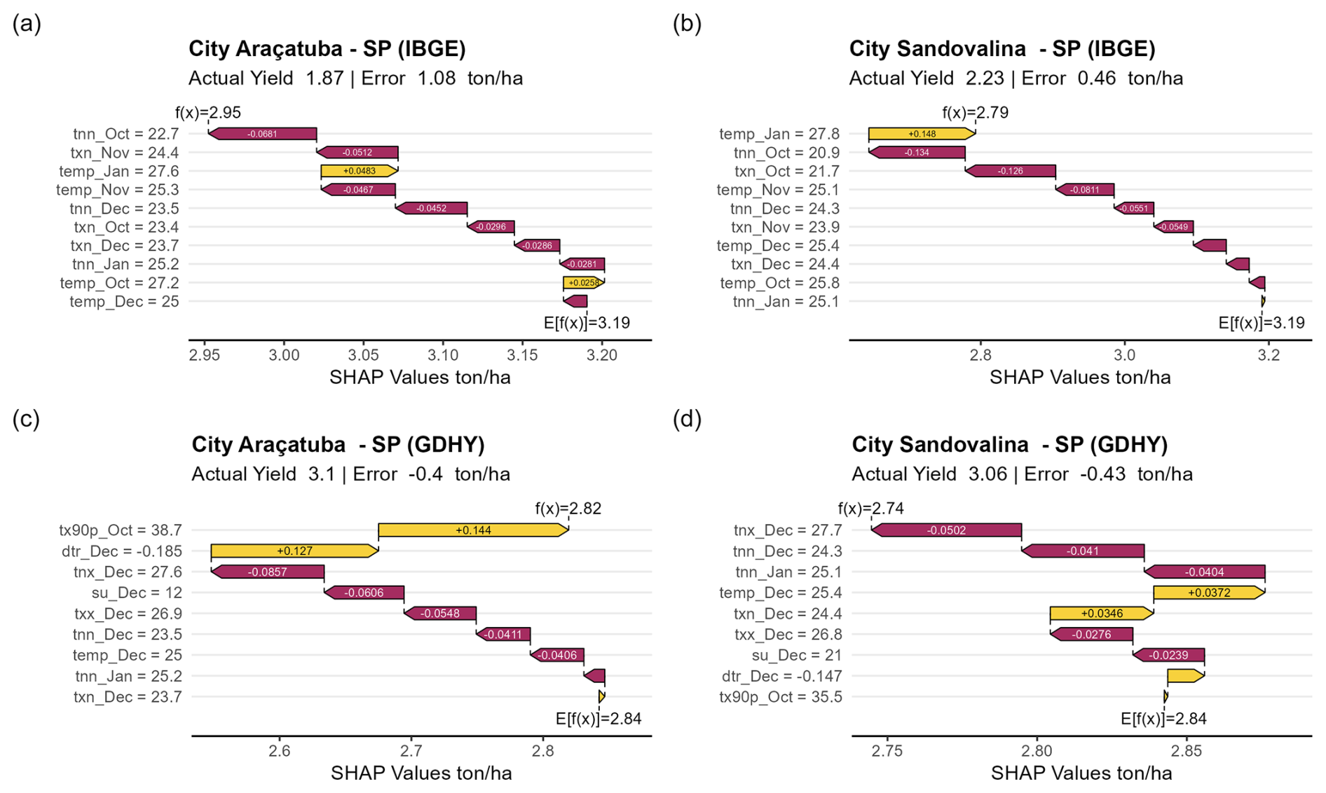
Figure 6 SHAP waterfall plot visualizing the key CID contributions to crop yield losses for the state of São Paulo (SP) in 2015, a drought year, with metrics for monthly maximum value of daily minimum temperature (tnx), minimum value of daily maximum temperature (txn), minimum value of daily minimum temperature (tnn), maximum value of daily maximum temperature (txx), percentage of days when tx > 90th percentile, standardized precipitation evapotranspiration index (SPEI), total precipitation (prcptot) and daily temperature range (dtr).

3.2 Determining thresholds and their significance

With the results of the selection of critical CIDs, we improved the understanding of the impacts on climate variables that significantly influence crop yield losses, considering different types of indices and critical periods. The insights obtained from the combination of random forest models applied to different datasets facilitate a robust understanding of climate–crop interactions and make it possible to compare what results the datasets have in common, increasing the results' reliability. However, the random forest model did not provide information on the values of each variable that are important and can help us define the threshold values of these indicators that are associated with an increased risk of crop yield losses.

To improve our understanding of how each climate extreme indicator was used for prediction, we used SHAP. This technique allowed us to extract insights from the results of a random forest model, thus providing a comprehensive perspective of the drivers of crop yield fluctuations. The results of SHAP-derived explanations revealed a clear pattern concerning the most influential variable that affects soybean yields. We highlight critical loss events by evaluating the model prediction for a particular city in a given year.

In 2019, an important widespread drought event was observed in Brazil and was considered a mega-drought that affected many regions of Brazil, especially the Paraná River basin Marengo et al. (2021). This drought extended into 2022 and occurred during a La Niña year. We highlight the model explanation for the state of Paraná considering two important agricultural municipalities, namely Marechal Cândido Rondon and Uniflor, as shown in Fig. 5.

The two datasets presented an agreement regarding crop yields below the expected value E[X]. However, they varied in terms of the magnitude of these losses. For the municipality of Marechal Cândido Rondon, the Deral yields are similar to the IBGE yields, 1.72 and 1.77 (Fig. 5), respectively. The predictions made by the two models were similar, and the main variables also performed similarly. High temperatures, represented by the maximum value of the daily minimum temperature in February, and low precipitation in December were the main drivers of losses combined with the 3-month SPEI in February.

For Deral, accumulated precipitation in December was also a significant driver of losses, and for IBGE, the 3-month SPEI was one in January. The other variables represented a negligible influence on crop yield losses. For the city of Uniflor, the actual Deral and IBGE yields were similar, 2.44 and 2.48 (Fig. 5), respectively. The main influences on crop yield losses were precipitation in December (prcptot_Dec) and high temperatures (tnx_Feb). The 3-month SPEI values in January and February can be considered redundant. Standardized indices refer to previous conditions; therefore, the values overlap in 2 months (December and January).

In 2014/15, a severe drought occurred in southeastern Brazil, causing an unprecedented water supply shortage in the Cantareira Water Supply System and affecting many cities in São Paulo (Deusdará-Leal et al., 2019). The drought had repercussions in many regions of the state of São Paulo. Therefore, we compared the IBGE and GDHY results for two municipalities in the state of São Paulo, Araçatuba and Sandovalina. The expected values of GDHY were lower than those of IBGE, and the two datasets diverged in yields below the expected value, i.e., IBGE indicated losses, and GDHY did not. According to a report by the Brazilian Ministry of Agriculture, Livestock and Food Supply (MAPA), the state of São Paulo was one of the most affected by losses in the agricultural year 2014/15 (MAPA, 2022). This result suggests that, although it has been suggested that GDHY is recommended in data-scarce regions (Iizumi and Sakai, 2020), using this dataset requires caution.

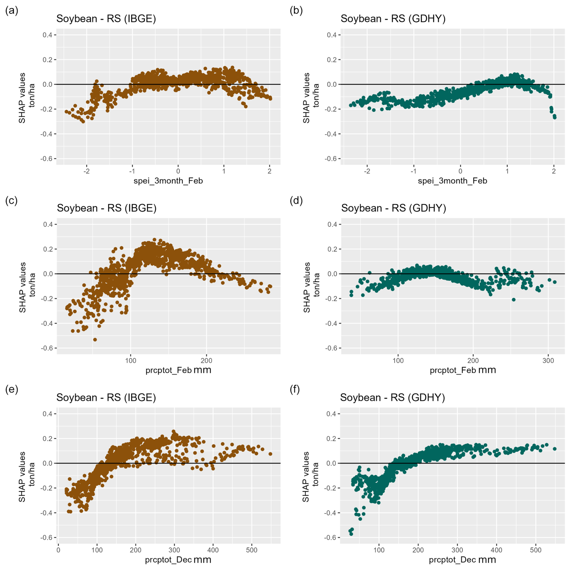
Figure 7 A comparison of the key CIDs derived from the Brazilian Institute of Geography and Statistics (IBGE) from 2013 to 2021 and the Global Dataset of Historical Yields (GDHY) from 2009 to 2016. Annual data aggregated at the municipal level were used to create a dependence plot for the soybean explanation model for validation data in RS. The data spanned 2013 to 2021 for IBGE and 2008 to 2016 for GDHY. The 3-month SPEI in February (spei_3month_Feb) for (a) IBGE and (b) GDHY, precipitation accumulated in February (prcptot_Feb) for (c) IBGE and (d) GDHY, and precipitation accumulated in December (prcptot_Dec) for (e) IBGE and (f) GDHY.

The SHAP methodology analyzes each prediction and shows how each variable was used in the model. This helps us create a partial dependence plot, which relates the variable's value with the impact in terms of crop yield losses represented by the SHAP value. This analysis is illustrated in Fig. 7, which shows partial dependence plots for the state of Rio Grande do Sul.

The comparison of the two datasets can be found in Fig. 7. The IBGE dataset shows that the 3-month SPEI in February can influence crop yield losses and has an upper and lower threshold. The lower threshold is −1.0. Values below this can represent losses of up to 0.2 t ha⁻¹. Generally, 3-month SPEI values below −1.0 are considered critical and are used as a reference for the severity of the drought (Chiang et al., 2021). Extreme wet conditions, with a threshold of 1, also affect crop yields in the RS state.

Excess rainfall can have the same impact as droughts (Li et al., 2019). However, little attention has been paid to this analysis. Our results suggest excessive precipitation can be responsible for up to 0.2 t ha⁻¹ of losses. More studies on this type of hazard are recommended. The cumulative precipitation in February presented a threshold of around 100 mm and a potential to cause losses of approximately 0.4 t ha⁻¹. The cumulative precipitation in December was the only indicator with a similar result in the IBGE and GDHY datasets. Regarding potential losses, both agree on a value of up to 0.6 t ha⁻¹; however, the threshold for IBGE is 150 mm, and for GDHY, it is 120 mm.

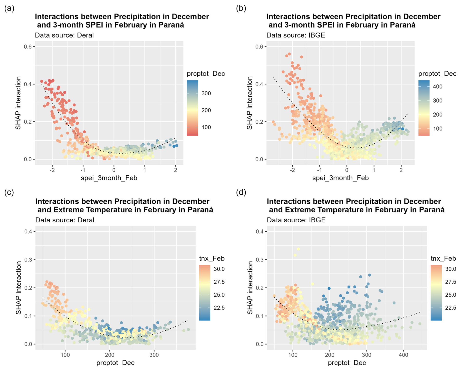
Figure 8 The 2D partial dependence derived from the Deral and IBGE data for the state of Paraná from 2016 to 2021 of the key climatic impact driver total precipitation in December (prcptot_Dec) with the most correlated CIDs and their combined impact on SHAP values (t ha⁻¹): considering the 3-month SPEI in February (spei_3month_Feb) and total precipitation in December (prcptot_Dec) and total precipitation in December (prcptot_Dec) and the maximum value of daily minimum temperature (tnn_Feb).

The patterns of crop yield losses observed in the region raise two main concerns. The first is that the severe crop yield losses presented in the previous examples have happened only once in the entire time series, representing an imbalance in the values of the dataset. One implication of this situation is that models may not have sufficient cases of severe failure to be trained adequately and may underestimate losses. The second concern is related to the decision to use these anomalous events. Possible solutions include using it for training, testing or removing it from the dataset. We opted to keep these events in the analysis with the warning that this might interfere with model performance. However, we wanted to evaluate the ability of the model to predict unprecedented loss events.

3.3 Evaluating combined hazards

The SHAP algorithm also allowed us to investigate the compound effect of climate indicators. In Fig. 8, we present the detection of compound event effects, considering the most important variable in the state of PR (prcptot_Dec) with four other considered important variables. We observed hot and dry compound events, characterized by high temperatures and a precipitation deficit, which have been cited as an increasing threat to food production (Zscheischler et al., 2018; Hamed et al., 2021).

This analysis also showed that precipitation in December was closely related to a 3-month SPEI in February. As discussed previously, this is expected since the SPEI considers previous conditions. However, it is essential to note that December is a critical month for droughts in PR and other states, such as Rio Grande do Sul (RS), Santa Catarina (SC) and Mato Grosso do Sul (MS).

Interestingly, indices based on the minimum daily temperature best reflected the impact of hot days. The maximum value of the daily minimum temperature in February (tnx_Feb) presented critical values of 27 °C. When minimum daily temperatures are high, it is likely that maximum temperatures are also high, and the difference between minimum and maximum daily temperatures is small; this is a possible explanation for why the daily temperature range (dtr_Oct) has a negative impact on crop yields when its values are close to zero. Since minimum daily temperature is associated with night temperature (Frich et al., 2002), our results corroborate the finding that warm nights pose a great threat to crop yields (Sadok and Jagadish, 2020).

Our use of RF with SHAP provides an advance by enabling quantification of the combined effect of multi-hazards on food production. In the realm of risk for food production, this method could be applied to explain the seasonal impact forecast made with composite indicators such as the integrated information system (IIS) (Cunha et al., 2018; Marengo et al., 2017). This approach is also readily applicable to other natural hazards, including landslides, floods and wildfires when utilizing with other datasets.

4 Conclusions

This study aimed to assess the impacts of climate extremes on food production using explainable ML algorithms. To achieve this goal, we extensively examined various datasets, focusing on soybeans and second-season maize in Brazil. Our data sources included the Department of Rural Economy, the Brazilian Institute of Geography and Statistics (IBGE), and the Global Dataset of Historical Yields (GDHY). Through an ML analysis, we examined the effects of climate extremes on crop yield production, ultimately providing critical insights for the agricultural sector. Our analysis incorporated data from several Brazilian states, including RS, SC, PR, SP, MS, MG and GO for soybeans and PR, SP, MS, MG and GO for the second season of maize.

We employed two machine models to achieve our research objectives. In the first model, we explored different combinations of input data, encompassing precipitation and temperature means, and more complex combinations, including precipitation, temperature means and extremes. This approach allowed us to determine the most relevant climate indices for the investigated regions. In particular, this experiment validated the robustness of our methodology, as it successfully identified climate indices of particular significance for regional studies.

We took the most relevant indices from the first experiment in the second model and then applied SHapley Additive exPlanations (SHAP) explanatory analysis to explore how the random forest model utilized the important indices to predict the impact of climate extremes on food production. This analysis revealed the impact of these indices and provided insights that may be crucial in establishing significant thresholds and guidelines for effective climate-driven decision-making.

In conclusion, our research exemplifies the potential of ML to understand and harness the influence of climate variables on food production. By determining the most pertinent CIDs and exploring their significance in a regional context, our findings contribute to a growing body of knowledge critical for informed decision-making, policy development and adaptive strategies in the face of climate change and its impact on agriculture. As demonstrated in our study, the combination of data-driven insights and advanced modeling techniques offers a valuable pathway toward ensuring food security under a climate change.