Tsunami detection methods for ocean-bottom pressure gauges

The real-time detection of tsunami waves is a fundamental part of tsunami early warning and alert systems. Several algorithms have been proposed in the literature for that. Three of them and a newly developed one, based on the fast iterative filtering (FIF) technique, are applied here to a large number of records from the Deep-ocean Assessment and Reporting of Tsunamis (DART) monitoring network in the Pacific Ocean. The techniques are compared in terms of earthquake and tsunami event-detection capabilities and statistical properties of the detection curves. The classical Mofjeld's algorithm is very efficient in detecting seismic waves and tsunamis, but it does not always characterize the tsunami waveform correctly. Other techniques, based on empirical orthogonal functions and cascade of filters, show better results in wave characterization but they usually have larger residuals than Mofjeld's. The FIF-based detection method shows promising results in terms of detection rates of tsunami events, filtering of seismic waves, and characterization of wave amplitude and period. The technique is a good candidate for monitoring networks and in data assimilation applications for real-time tsunami forecasts.

1 Introduction

Tsunami early warning and alert system operations are based on the rapid earthquake characterization in terms of magnitude and hypocenter after which alerts are typically given based on a decision matrix or on databases of precomputed tsunami propagation scenarios; the forecast can then be confirmed, updated or canceled based on additional earthquake information (e.g., focal mechanism, moment tensor, finite fault models) and sea level measurements (Titov et al., 2005; Duputel et al., 2011; Lomax and Michelini, 2013; Amato et al., 2021). The latter are crucial for the rapid characterization of tsunami waves, which are monitored from tsunami warning centers by means of coastal tide gauges and/or ocean-bottom pressure gauges (OBPGs) (Rabinovich and Eblé, 2015).

Historically, the first tsunami-recording instruments were coastal tide gauges, for which self-recording variants have been available since the 1830s (Matthäus, 1972). However, such instruments measure the sea level in close proximity to the coast. For this reason, they are not the primary choice in the context of tsunami detection, even though they can be used for early warning purposes wherever no other instruments are located and real-time detection algorithms for tide gauges have been developed (Bressan et al., 2013; Lee et al., 2016). Furthermore, the tsunami evolution at coastal locations is deeply influenced by its nonlinear interaction with the local bathymetry and topography.

Conversely, these site effects are negligible in the case of measurements of tsunami waves in deep-water environments using OBPGs. By virtue of being located at the bottom of the ocean, these instruments only detect long wave signals, such as tsunamis and tides, filtering out naturally the most superficial oscillations; moreover, the open-ocean tsunami evolution is less affected by complex interactions with coastal morphology and is mostly a linear phenomenon. Thus, the signals from ocean-bottom measurements are a superposition of

1. tidal oscillations, dominated by diurnal and semidiurnal periods, which are the main contribution to the energy of the signal;

2. random oscillations in the same frequency range of tides, not accounted for by harmonic analysis;

3. tsunami waves;

4. changes in pressure due to displacement of the ocean bottom.

This last case is evident for gauges subjected to seismic shaking, like for instruments located relatively close to the earthquake source zone, for which seismic and tsunami waves may not be well separated in the recordings, making the extraction of the tsunami wave quite challenging. Thus, techniques able to separate the two contributions are necessary for instruments located near the potential earthquake sources (Williamson and Newman, 2019). For detailed discussions on the nature of deep-ocean pressure measurements, we refer to the many detailed works in the literature, such as Rabinovich (1997), Goring (2008), Mungov et al. (2013), and Rabinovich and Eblé (2015).

OBPGs can be classified based on the transmission technology they used, either through cable or through acoustic transmission. Cabled instruments transmit data as soon as they are acquired through cable to research or data centers, where they are analyzed for both early warning applications and later studies. Cabled instruments are commonly used for real-time forecast (Tsushima et al., 2007) and data assimilation applications (Wang et al., 2019a), and they are used as part of the DONET (Kawaguchi et al., 2008) and S-NET (Mochizuki et al., 2018) networks deployed around the Pacific coasts of Japan to monitor both local and far-field earthquakes and tsunamis.

OBPGs with acoustic transmission are the ones used in the Deep-ocean Assessment and Reporting of Tsunamis (DART) network (National Oceanic and Atmospheric Administration, 2005; Titov et al., 2005), composed of a variable-in-time number of OBPGs operating around the Pacific, northeastern Indian and north Atlantic oceans, each of which continuously transmits pressure data to a buoy located at the sea surface, which then transmits data to the tsunami warning center. The data transmission frequency between the pressure gauge and the buoy increases in the case of an event, which can be triggered by an automatic detection or an external prompt. The recorded pressure changes can then be converted to sea level variation and incorporated into the tsunami forecast with different methods, such as real-time source inversion (Titov et al., 2003; Tang et al., 2009), data assimilation methods (Maeda et al., 2015; Wang et al., 2017, 2019a, b; Heidarzadeh et al., 2019; Wang et al., 2021) or recently proposed Bayesian approaches (Selva et al., 2021b).

Lastly, we mention that another possible instrument for direct sea level measurement offshore is the GPS buoy (Kato et al., 2000). In this case, a GPS receiver is placed on a stable buoy and data are analyzed at a ground base station using real-time kinematics (RTK) to obtain the relative vertical motion of the buoy. GPS buoys have been used for real-time tsunami inversion as well (Yasuda and Mase, 2013).

The purpose of this work is to test and compare real-time tsunami detection methods from the literature that have been applied to real data acquired by OBPGs. In particular, some techniques are chosen and then applied to past OBPG data as if it would happen in real time. The first technique is the one proposed by Mofjeld (1997). Since every DART station has the algorithm implemented on board, the technique has a long history of applications and analysis of its properties (Beltrami, 2008, 2011; Chierici et al., 2017). It has to be noted that fourth generation DART (DART 4G) also includes an additional algorithm which allows the automatic separation of seismic shaking and tsunami waves, exploiting the higher sampling rate (https://www.ndbc.noaa.gov/dart/dart.shtml, last access: 24 February 2025). For that, 1 s sampling rate data are used (Christopher Moore, personal communication, 2024). Since not enough information regarding DART 4G is publicly available, in this study, we do not deal with this algorithm, but rather test the other algorithms on largely available DART data with sampling times of 15 s. Many of them are currently operational. It also has to be noted that even the onboard sampling rate is higher, the ordinary transmission rates are lower, and the onboard computing capability is generally limited, in each case to limit the battery consumption. Thus, it is desirable to have a detection algorithm that works for relatively low sampling rates.

The other techniques presented and tested are the detiding through empirical orthogonal functions (EOFs) (Tolkova, 2009, 2010) and the tsunami detection algorithm (TDA) developed by Chierici et al. (2017). Lastly, a new technique, similar to the one developed by Wang et al. (2020), is presented. This new technique is based on the fast iterative filtering (FIF) technique (Cicone, 2020; Cicone and Zhou, 2021) and the IMFogram time–frequency representation (Barbe et al., 2020; Cicone et al., 2024a).

These applications include tests on background signals, i.e., signals where no evident earthquake or tsunami oscillation is present, and on records acquired during the generation and propagation of past events. With these analyses, we are able to characterize each technique in terms of their filtering capabilities for both high- and low-frequency disturbances. Tests on past events' signals allow us to quantify the detection rates of each technique and to evaluate how they would perform in an early warning setting through simple detection scores. Moreover, we propose simple possible criteria to determine optimal detection thresholds for each detection method, based exclusively on real OBPG data.

The four techniques, which we will refer to as MOF (short for Mofjeld), EOF, TDA and FIF for brevity, are described in their basic mathematical structure in Sect. 2. Applications are then shown in Sect. 3 in order to study how the techniques behave on signals with and without tsunamis.

2 Algorithms for real-time tsunami detection

2.1 MOF algorithm

DART stations in the NOAA monitoring network are equipped with an automatic tsunami detection algorithm, described by Mofjeld (1997). The algorithm compares the pressure recorded at each instant with a prediction computed from the previously acquired data. If the absolute difference between these two values exceeds a given threshold, this is considered a detection of a sea level anomaly.

The predicted value is found by using Newton's forward polynomial interpolation formula:

$$\begin{array}{}\text{(1)}& H_{\mathrm{p}}\left(t^{\prime }\right)=\sum _{i=\mathrm{0}}^{\mathrm{3}}{w}_i\stackrel{\mathrm{‾}}{H}\left(t-i\mathrm{d}t\right),\end{array}$$

where t^′ is the prediction time set to t + 5.25 s, where t is the time of most recent measurement used to compute the interpolating polynomial; $\stackrel{\mathrm{‾}}{H}$ is the 10 min moving average of pressure data; and dt = 60 min. For the default parameters, the following can be shown.

$$\begin{array}{}\text{(2)}& \begin{array}{l}{w}_{\mathrm{1}}=+\mathrm{1.16818457031250}\\ w_{\mathrm{2}}=-\mathrm{0.28197558593750}\\ w_{\mathrm{3}}=+\mathrm{0.14689746093750}\\ w_{\mathrm{4}}=-\mathrm{0.03310644531250}\end{array}\end{array}$$

The technique is particularly suitable for onboard implementation due to its very simple mathematical formulation, computational efficiency and low requirements in terms of data needed for the prediction, since little more than the previous 3 h of measurements is needed.

We note that the most recent point used for extrapolation is 5 min before the current time. If a tsunami signal has a period longer than that, the averaging operation will not be able to remove it, so the extrapolation will be affected by the presence of the tsunami. The result is that residuals produced by Mofjeld's algorithm deviate in terms of amplitude and period from the tsunami waveform. The problem is addressed by Beltrami (2011), showing that a better agreement between the residual and the tsunami waveform may be obtained by adopting a longer prediction time. However, this results in a much smaller signal-to-noise ratio. The technique has no built-in method to filter out high-frequency components, such as random noise and seismic waves.

2.2 EOF detiding

The use of empirical orthogonal functions (EOFs) for detiding has been introduced by Tolkova (2009, 2010). The method is based on the application of principal component analysis to a pressure record ζ(t) as follows:

1. Extract from a long time series N segments of length M.

2. Compute the covariance matrix,

   $$\begin{array}{}\text{(3)}& C_{ij}=\sum _{k=\mathrm{1}}^N\left[\mathit{\zeta }(q_k+i-\mathrm{1})-a_k\right]\left[\mathit{\zeta }(q_k+j-\mathrm{1})-a_k\right],\end{array}$$

   where q_k is the index where the kth fragment starts and a_k is the average of the kth fragment.

3. Compute the EOFs e_i as the eigenvectors of the matrix $C_{ij}+C_{M+\mathrm{1}-i,M+\mathrm{1}-j}$.

It has been shown by Tolkova (2009) that the first few EOFs are sufficient to reconstruct the tidal component of the sea level signals. Furthermore, Tolkova (2010) shows that these bases have a universality property. In fact, if we compute the EOFs for data obtained in different locations, the residual produced by detiding a signal has the same amplitude whatever basis we use. For this reason, once we have data from a tsunameter in a basin, the technique may be applied to detide any signal from any other instrument within the same basin.

The explanation proposed by Tolkova (2010) hinges on the fact that the periods of the diurnal and semidiurnal tidal components, captured by the first few EOFs, are the same in every position in the global ocean. Since tides are obtained by projection, the differences in amplitude between different basis function sets have no effects on the decomposition. On the other hand, the tidal fine structures, i.e., tidal oscillations of shorter periods such as 6 and 8 h, are location-specific and are thus removed with this technique. It should be noted also that the universality of the main tidal components has been shown empirically, but we lack a rigorous justification. Thus, the property may not be valid for data acquired very far from the sensors used by Tolkova (2010).

To apply the technique to real-time tsunami detection, a 1-lunar-day-long (24 h 50.4 min) basis is used. At each time step

1. the signal average is subtracted from the data;

2. tides are extracted by projecting the last-acquired data onto the EOF basis;

3. a residual is computed by subtracting computed tides from the original signal;

4. the last residual point is compared with a given threshold;

5. once a new measurement is acquired, the computation is repeated on the new 1-lunar-day time window that ends at that measurement.

Since tides are obtained by projection, the results of the computations are unaffected by multiplying any of the basis functions by an arbitrary constant.

The technique is computationally efficient, since computing the tides s by projection of a signal η can be done by a simple matrix–vector product like

$$\begin{array}{}\text{(4)}& s=\mathbf{E}{\mathbf{E}}^T\mathit{\eta },\end{array}$$

where the matrix E has the EOF basis vector e_i as columns. It has also been shown that using seven elements for the basis minimizes errors for the chosen signal length. In this work, the basis is obtained from DART 46414 in the period between 6 June 2018 and 8 June 2022, since it presents no discontinuities or missing data. The obtained basis is shown in Fig. 1.

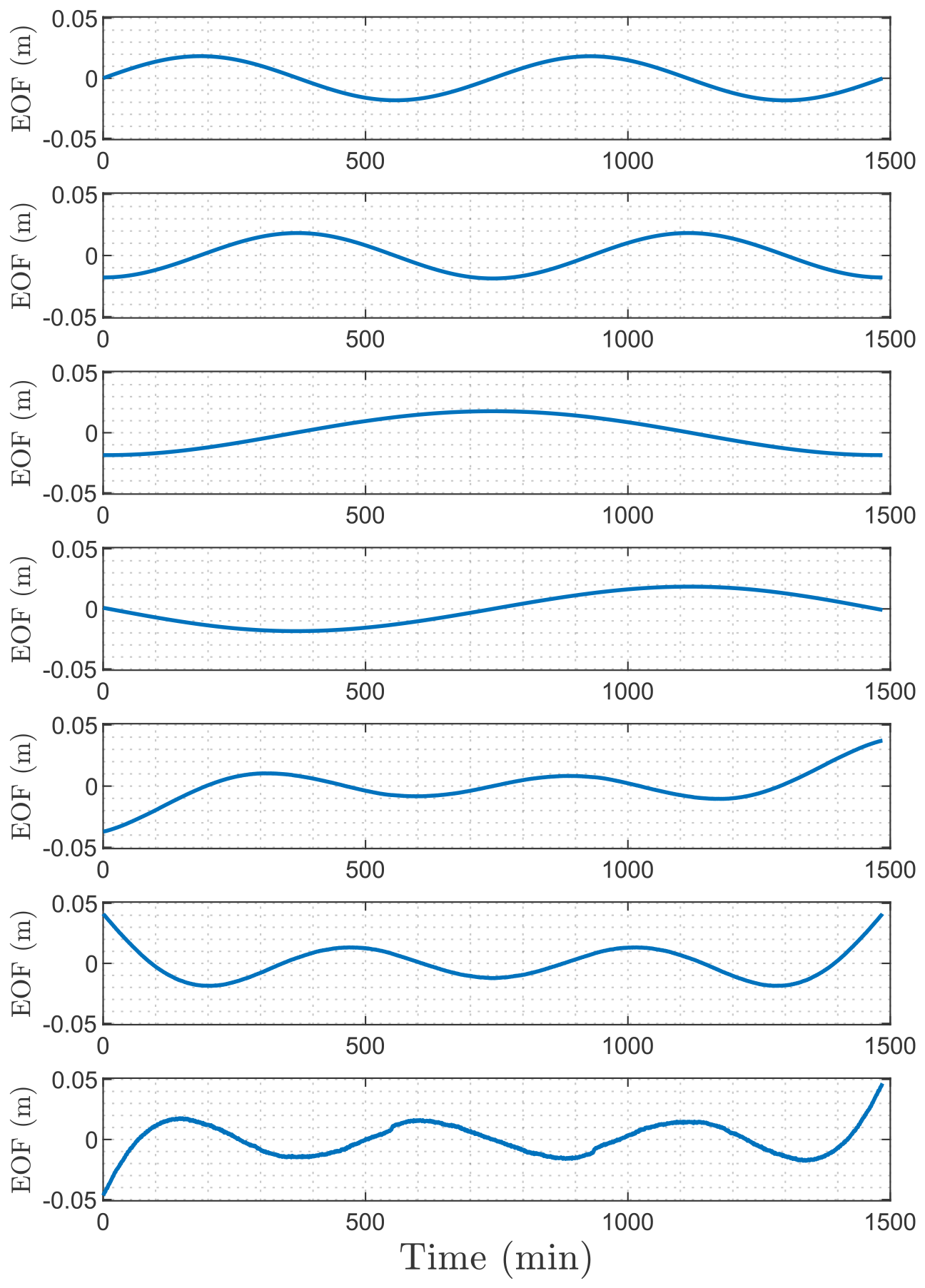
Figure 1 Empirical orthogonal functions computed for DART 46414 (in the period 6 June 2018–8 June 2022) and used for EOF-based detection. The DART station is located southeast of Chirikov Island in the Gulf of Alaska. We note that the vertical scale is arbitrary. Since the tides are computed by projection on this basis, any multiplicative scaling of any EOF would have no effect on the computed tides.

2.3 TDA

The tsunami detection algorithm (TDA), introduced by Chierici et al. (2017), has a modular structure, which includes tide prediction and signal filtering. Each time a new pressure measurement is acquired, tides are removed using a harmonic model (Pawlowicz et al., 2002) with precomputed coefficients. After that, a spike detection algorithm is used to eliminate isolated spikes. Lastly, the residual time history is bandpass-filtered using a finite impulse response (FIR) filter. Since the TDA is designed to work in real time, which is only utilizing previous data, a mirroring boundary condition is applied to the signal before filtering.

The TDA has been specifically developed to be as computationally efficient as possible, and the processing at each time step requires only a few thousand floating-point operations. Furthermore, the modularity makes it very easily adaptable to different operational conditions. On the other hand, requiring precomputed tidal coefficients puts a constraint on the applicability, since a relatively long time series, on the order of a few months, is needed at the position of the instrument. Thus, the technique as described by Chierici et al. (2017) cannot be applied to instruments which have been deployed too recently or have recorded jump discontinuities. Both of these events occur in the case of DART instruments, since they are periodically resurfaced for maintenance and downloading raw data and then deployed again in a different position. The case of jump discontinuities, due to resurfacing or other reasons, usually requires ad hoc processing, as in the case of very long (e.g., multiannual) trends (Mungov et al., 2013). Techniques to account for these occurrences in real time need further investigation and are outside the scope of the present work. Whenever such a case is present for a signal in our datasets, TDA is not applied to it. An intermediate situation may occur where enough data to compute a set of tidal coefficients are available but not enough to remove tidal oscillations completely. In these cases, the residual produced by the technique may have amplitudes of several centimeters that may produce false detections even in the absence of any anomaly. Local tidal ranges may also play a role, since areas with much larger tidal ranges are expected to have larger residuals. Given the modularity of TDA, different detiding techniques can be employed in the place of the harmonic model presented (Consoli et al., 2014). However, this is outside the scope of the present analysis.

In this work, tidal coefficients are computed using UTide (Codiga, 2011) from at least 2 months of data ending a few days before the time interval of interest in each case. For the harmonic filter, Chierici et al. (2017) use a 4000-point FIR bandpass filter with a [2 min,120 min] or [4 min,120 min] period window. Here, we use the second window, since we are mainly interested in applications to tsunamis of tectonic origin. Furthermore, filtering using this period band happens to filter out the frequencies which may be contaminated by infragravity waves (Mungov et al., 2013).

2.4 FIF-based tsunami detection

The FIF technique (Cicone, 2020) is a data-driven signal analysis technique for decomposing nonlinear and nonstationary signals into simple oscillatory components. The decomposition is additive, so a signal s(t) can be written as

$$\begin{array}{}\text{(5)}& s\left(t\right)=\sum _{k=\mathrm{1}}^N{I}_k\left(t\right)+r\left(t\right),\end{array}$$

where I_k are called intrinsic mode functions (IMFs) and r(t) is the residual. Each IMF satisfies the following properties:

1. The number of zero crossings and the number of relative extrema differ at a maximum of one unity.

2. The envelopes of relative maxima and relative minima are symmetric with respect to zero.

A function with such properties can be regarded as a generalization of a Fourier mode f(t)=A(t)cos (θ(t)), where the amplitude A(t) can vary with time and the phase θ(t) is allowed to be nonlinear (Huang et al., 1998).

The most common method to decompose a signal into IMFs is the empirical mode decomposition (EMD), introduced by Huang et al. (1998). However, the FIF method has some properties that make it preferable. In particular, it is more robust to noise (Cicone et al., 2016), it is not prone to mode mixing (Cicone et al., 2024b), and it generates no unwanted oscillations as defined by Cicone et al. (2022). The FIF shares some of these good properties with the ensemble empirical mode decomposition (EEMD; Wu and Huang, 2009), but for EEMD this comes with a severe increase in computational cost. In contrast, FIF can be formulated using fast Fourier transform (FFT) (Cicone and Zhou, 2021), making it numerically efficient. To perform a time–frequency analysis of a signal, FIF is complemented by the IMFogram technique (Barbe et al., 2020; Cicone et al., 2024a). From the IMFogram, instantaneous amplitudes and frequencies are computed for each component from the envelope of the absolute value of extrema and the distribution of zero crossings, respectively.

The tsunami detection strategy we propose is as follows:

1. Take the last 3 h of acquired sea level data.

2. Remove the long period trend by robust polynomial fit (Street et al., 1988).

3. Decompose the residual using the FIF technique.

4. Sum the IMFs with frequency content, computed with the IMFogram method, lying within a chosen frequency band.

5. Compare the last point of the obtained signal with a chosen amplitude threshold.

6. Repeat from step (1) once a new sea level measurement is acquired.

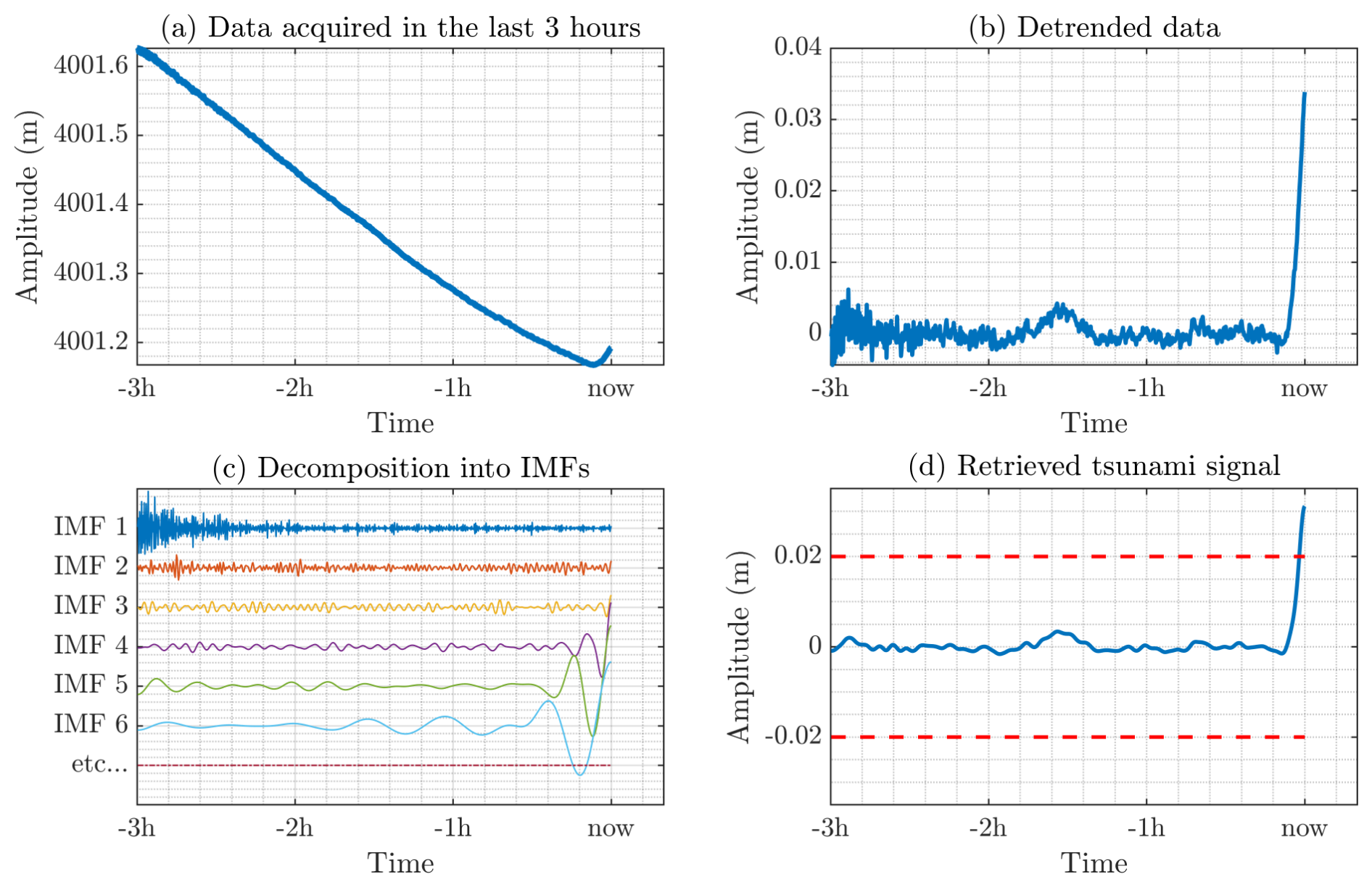
Figure 2 Example of FIF-based decomposition: (a) the last 3 h of data is taken, (b) detrended through polynomial fitting and (c) decomposed using FIF, and (d) the sum of components in the chosen frequency band (periods between 4 and 180 min) are summed. Data from DART 32413, during the 16 September 2015 Illapel tsunami. The generating earthquake occurred at 22:54:32 UTC, while “now” in the plot refers to 4 h 43 min after origin time.

The reason for which the tidal trend is removed through polynomial fit lies in the ability of IMFs to capture components with variable frequency. Just after the arrival of a tsunami wave, as in the example in Fig. 2, using FIF on raw data before detrending may not separate the tsunami wave from tides. For 3 h long signals, polynomials of degree 3 seem to be the most appropriate. In terms of frequency band, in this work we retain components with periods between 4 and 180 min, which represent a conservative window for preserving all components related to earthquake-generated tsunamis. Nonetheless, we point out that the combination of FIF and IMFogram techniques is quite robust with respect to the choice of both their parameters and the chosen period window. An example of the procedure for one time step is shown in Fig. 2.

The decomposition step in Fig. 2 deserves further comments in regards to the presence of non-causal oscillations in the components, i.e., non-physical oscillations before the tsunami's arrival. Firstly, we point out that this effect is not exclusive to FIF (or FIF-like) decompositions and it can be observed also in classical Fourier trigonometric series. One example can be found in Figs. 18 and 19 in the work by Tolkova (2009). Secondly, the tsunami component of the signal is obtained by summing components within the chosen frequency band. In doing so, the additional oscillations cancel out, as shown in the example in Fig. 2. Thus, they have no effect on the obtained residual. Nonetheless, this effect could be avoided using a different set of parameters for the FIF decomposition. Given the robustness of the technique the results of the present work do not depend on this choice. Therefore, the determination of optimal parameters is left for future works.

A similar detection technique based on data-driven signal decomposition was proposed by Wang et al. (2020). The FIF-based detection proposed here differs in two aspects. Firstly, they use the more computationally expensive EEMD-based signal decomposition. Despite having two more steps, namely trend removal and frequency computation, than the technique by Wang et al. (2020), the numerical efficiency of FIF makes our algorithm faster overall. Secondly, Wang et al. (2020) a priori choose which components represent the tsunami, while we choose them based on the frequency content computed at each time step.

3 Performance comparison

To test the algorithms described in the previous sections, raw data from OBPG were retrieved from the Unassessed Ocean Bottom Pressure (highest available resolution) catalog available on NOAA's website (https://www.ngdc.noaa.gov/thredds/catalog/dart_bpr/rawdata/catalog.html, last access: 24 February 2025). For background analyses, DART data from New Zealand's network were also used, which are available from GeoNet's website (https://tilde.geonet.org.nz/, last access: 24 February 2025).

All the techniques we consider here are amplitude-based – i.e., they process the most recent available portion of data and a detection is triggered based on the amplitude of the last point of the processed signal. To characterize the properties of each technique, we analyze the time history made of these last points processed at each time step. We will refer to these time series as “detection curves”. The content of the detection curves is a superposition of residuals of the analysis and any component that is not filtered in the processing. However, the specific nature of these contributions differs among the techniques. For example, MOF only removes long-term trends, so detection curves contain oscillations from seismic and tsunami waves and random noise. In the case of techniques with a model-based tide-removal algorithm, such as EOF detiding and TDA, there may be contributions to the detection curves due to unmodeled tidal components. The role of random instrumental noise is reduced wherever high-frequency filtering is used, e.g., for TDA and FIF, but not completely eliminated, since detection curves include only the last point of each analysis and are thus prone to errors from the boundary treatment. FIF detection curves may also be affected by errors in the polynomial fit. In every case, the characteristics that we want from an ideal detection curve are to have an amplitude that increases in correspondence with the passage of a tsunami wave while remaining below a given threshold anywhere else. Also, it is desirable to have them symmetrically distributed around zero. For example, in a detection curve with a negative bias, leading trough waves may be detected even if they have amplitudes smaller than the detection threshold, while leading crest waves may not be detected even if larger than the threshold.

Each technique is applied to two different datasets. The first dataset includes time series consisting only of tides and random noise, which we will refer to as “background signals”. Among these we have five time series of 1-month length, where the first characteristics of each technique are shown, and 16 signals from different instruments recorded simultaneously in the absence of tsunami events. From these analyses, we are able to characterize the properties of the residual. The second includes day-long signals recorded at DART stations during real tsunami events to check if the techniques are able to detect tsunamis and if and when a detection is false or triggered by seismic shaking.

We note here that the applications have been carried out on raw pressure data and that all data and plots are expressed in meters of equivalent water through the equivalence 1 dbar = 1 m. The equivalence is only valid whenever the vertical pressure profile in the water column can be assumed to be hydrostatic. While this is usually the case for earthquake-generated tsunamis, there are cases where it fails, such as the case of coupled air–sea waves (Okal, 2024). While taking this into account is fundamental for the proper characterization of the tsunami source, it does not have an effect on the properties of the detection algorithm. However, any integration of the techniques tested here into any alert system must take into account that tsunami waveforms observed in detection curves represent pressure signals and any use in data assimilation or forecast methodology must correctly convert it into sea level time series.

3.1 Background signal analyses

For the analysis of the background signal, we started by selecting five time series of 1-month length, according to the following criteria:

1. no visible seismic or tsunami oscillations;

2. no instrumental spikes, holes or discontinuities;

3. part of a deployment long enough to accurately compute tidal coefficients needed for TDA.

Furthermore, the different time series are taken from instruments installed in different areas around the Pacific Ocean to avoid biases due to regional features.

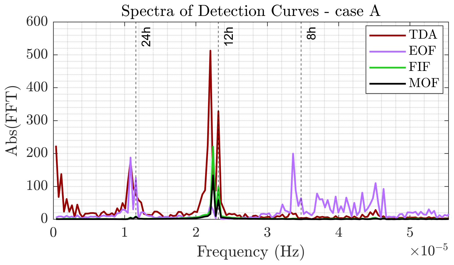
Here, we illustrate the analysis by considering the signal chosen from DART 46414 (Fig. 3), whose detection curves for each technique are shown in Fig. 4. All detection curves show some residual oscillations, though of different amplitude and spectral content, as shown by the spectra in Fig. 5. The EOF detection curve has peaks for periods around 24 h, i.e., the residual from the main diurnal component, and 8 h, which may be related to the fine structure of tidal oscillation that is not captured by the algorithm (Tolkova, 2010). TDA has the main periods around 12 and 24 h, showing that the main contribution to the residual is given by the difference between predicted and observed tides. MOF and FIF detection curves also have a spectral peak around a period of 12 h but with a lower amplitude. Also, contrary to EOF, they have a mostly flat spectrum far from the semidiurnal frequency band.

Figure 3 Raw data from DART 46414 for the month of August 2019.

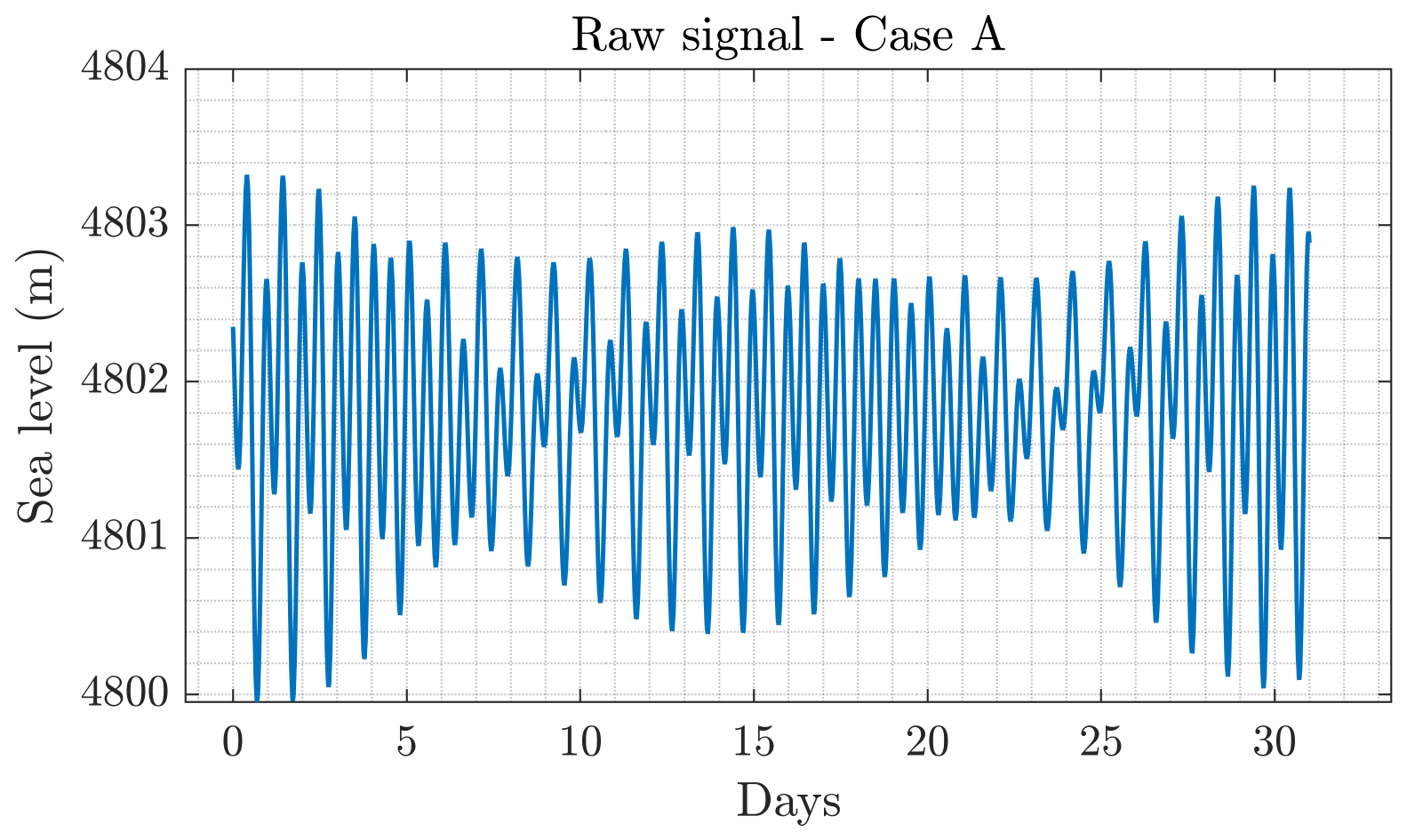
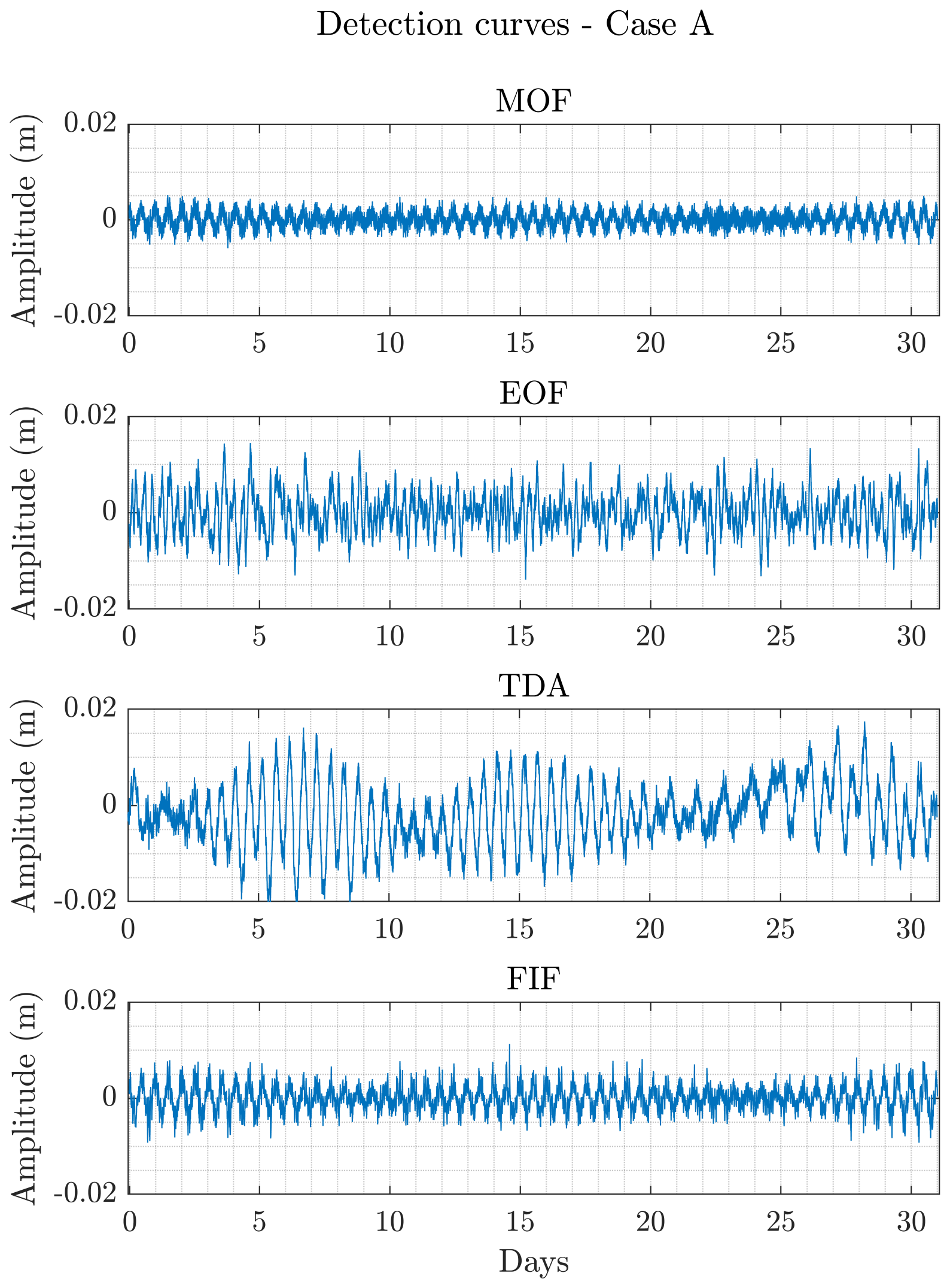
Figure 4 Detection curves for each detection technique for DART 46414 from August 2019 (Fig. 3).

Figure 5 Spectra, computed as absolute values of the fast Fourier transform (FFT), for each detection curve in Fig. 4 relative to data from DART 46414 from August 2019 (Fig. 3).

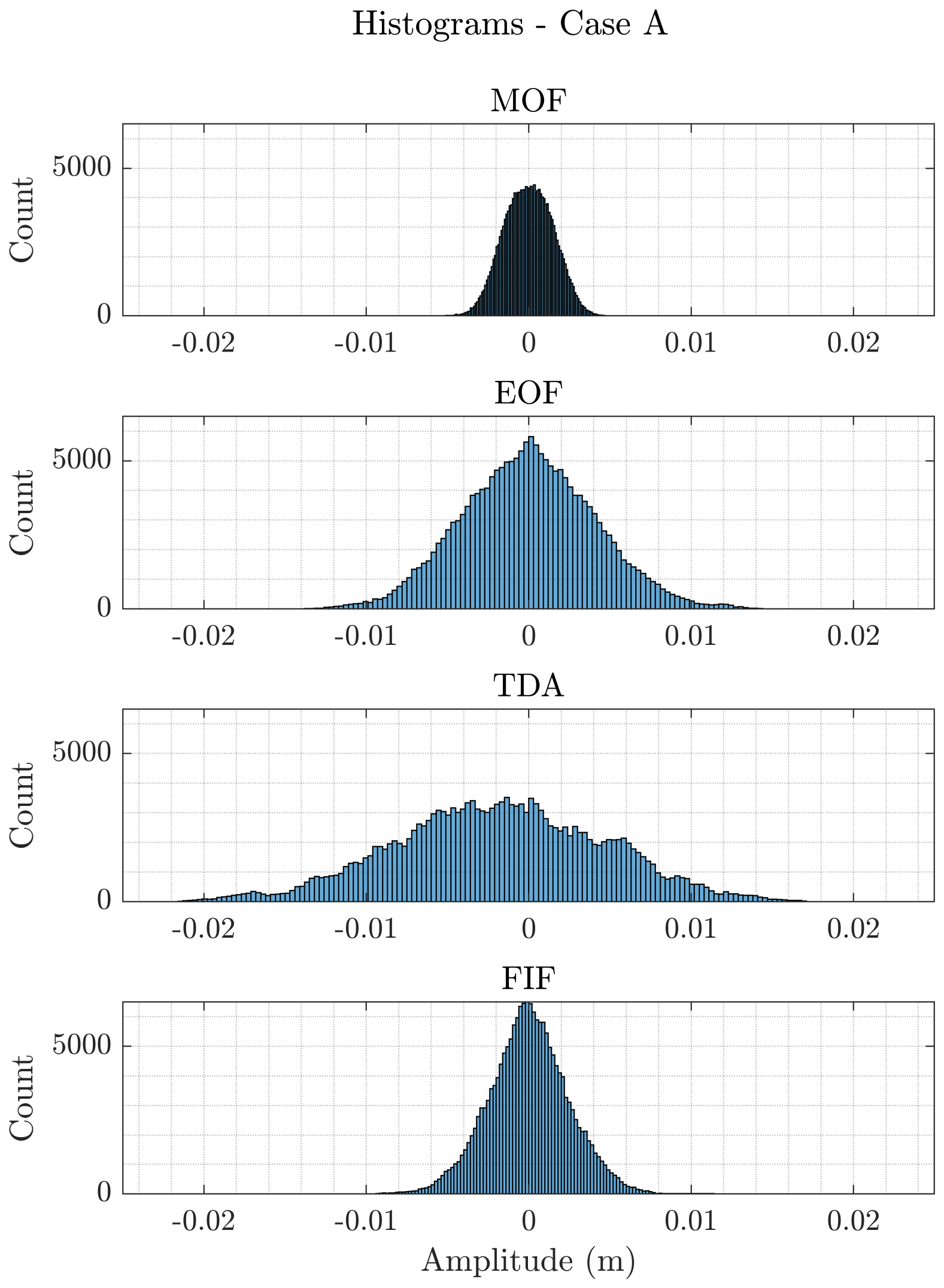
It is also interesting to look at the amplitude distribution of the prediction around zero. From the histograms in Fig. 6, we can notice that the MOF technique has the narrowest distribution, since it is able to remove the long-term trends entirely, with the only contribution to the detection curve being the random noise, as pointed out before. FIF has a very peaked distribution, indicating that the detection points checked at each time step do not deviate much from zero. On the other hand, EOF and TDA have a wider distribution, which shows that a larger number of values are further away from zero. For TDA, it can also be noticed that the histogram is not centered around zero; i.e., the points in the detection curve are distributed asymmetrically due to the fact that the predicted tides are above the raw data.

Figure 6 Histograms of each detection curve in Fig. 4, relative to data from DART 46414 from August 2019 (Fig. 3).

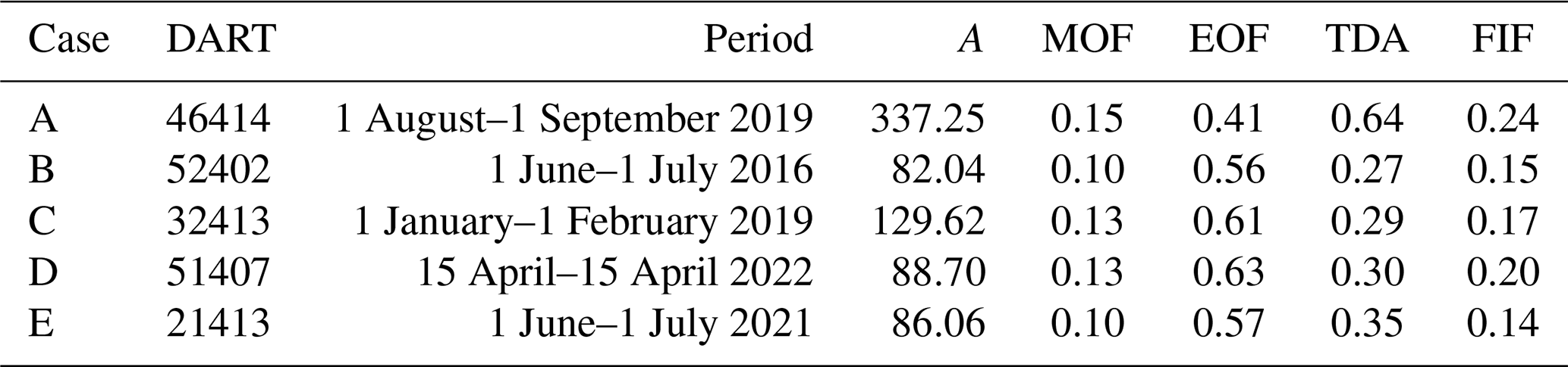
The conclusions made for the case in Fig. 3 can be generalized to the analysis of the other four background signals. The variability in the detection curves for all five cases can be measured by their maximum range of variability and standard deviation, reported in Tables 1 and 2, respectively. In each case, MOF produces the narrowest distributions, both in terms of maximum variability, which is around 0.5 cm from zero, and in terms of standard deviation. FIF shows a larger variability for both metrics compared to MOF but smaller than the other techniques, remaining within 1.2 cm from zero at each time. EOF is the technique with the largest standard deviations from the origin on average, followed by TDA and then FIF and MOF, with the exception of case A, where TDA has a larger standard deviation than EOF. This may be caused by the large tidal range in case A (see Table 1), which results in less accurate tide prediction.

Table 1 Maximum peak-to-peak amplitude, indicated as A, of raw data and maximum variability range of detection curves for each technique in each background case. All quantities are expressed in centimeters.

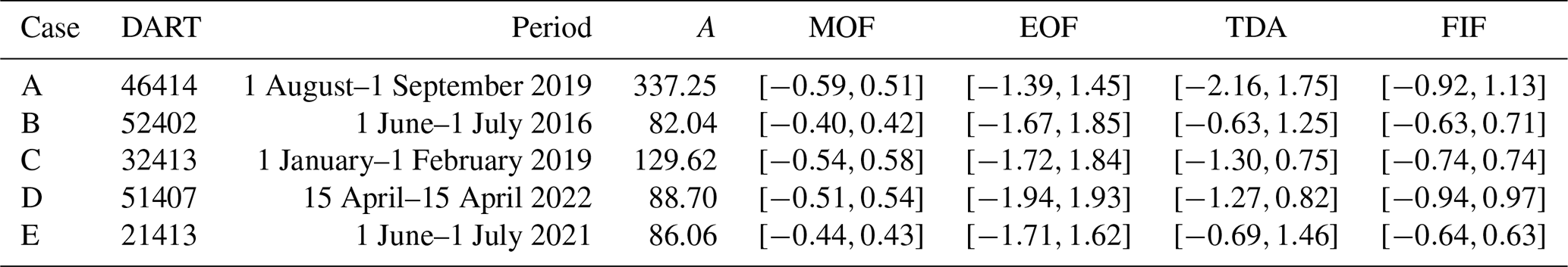
Table 2 Standard deviation expressed in centimeters for each technique in each background case.

The asymmetric amplitude distribution of TDA is observed in all cases. Cases A, C and D are negatively skewed, while cases B and E are positively skewed. In contrast, the other techniques are approximately symmetrical in every case. For these five time series, the threshold of 3 cm, commonly used in DART OBPGs (Mofjeld, 1997; Rabinovich and Eblé, 2015), produces no false detection and seems to be a highly conservative choice. In fact, a 2 cm threshold would result in false detections only for TDA in case A. For MOF and FIF, the threshold may be lowered to 1 and 1.5 cm, respectively. Plots for cases B, C, D and E, analogous to Figs. 3 to 6, are reported in the Supplement. Furthermore, the analysis of these five cases has been used to have a first-order evaluation of the sensitivity of TDA to the amount of data used to compute tidal coefficients. We determined that an amount of data between 7 to 9 months results in the narrowest detection curves for TDA. Details about this analysis are reported in the Supplement.

We should point out that the presented background analysis takes into account geographical variability only weakly, since the five signals are from different points in time. Furthermore, multiple tsunamis occurred and were detected during those time windows. This in principle may lead to misinterpretations of the results, and weak anomalous oscillations could be attributed to those events. To verify the properties of the detection algorithm accounting for these factors, we set up another test. In this case, we selected data following these criteria:

• Signals were acquired simultaneously by different DART stations.

• The considered DART stations were located in various locations to have maximum geographical coverage.

• The raw data preceding the signal at each station should be long enough to accurately compute tidal coefficients for TDA.

• The considered time window should include no tsunami in the regions where the DART stations are located.

Accordingly, we chose the period between 8 and 27 April 2021. We use data between 1 August 2020 and 1 April 2021 to compute tidal coefficients. In this period, we found 19 DART stations that met the data amount requirements, 3 of which were excluded due to the presence of isolated spikes in the considered time frame. During this period, only one tsunami is reported by NOAA National Centers for Environmental Information (2025)'s global tsunami catalog, related to the eruptive activity of La Soufrière volcano on the island of Saint Vincent. The catalog reports a maximum runup of 0.1 m on the island. Since only 2 of the 16 stations are in the Atlantic Ocean and the closest is located at ∼ 1000 km, we assume that the signals are unaffected by the tsunami waves.

In Fig. 7, we show the signal average and the absolute extrema of each detection curve for each technique. For the most part, the results reproduce what we observed in the previous background examples. MOF and FIF have narrower and more symmetric distributions around zero than EOF and TDA, with no curve that ever reaches an absolute amplitude of 1.3 cm. On the other hand, TDA's signal averages tend to be larger in absolute value, meaning that the amplitude distribution of the amplitudes is skewed away from zero. The results for EOF in the case of New Zealand's DART stations are noteworthy, since they have the largest-amplitude residual out of all the background tests: 3.2 and 2.9 cm maxima for stations NZC and NZE, respectively. A possible reason might be that these stations are significantly further away than most of the others from the position of the DART station used to compute the EOF basis, located in the Alaskan Aleutian arc, and the New Zealand area was not covered in the empirical tests by Tolkova (2010), since data were not available at the time. Although one reason for the difference could be found in the distance between these stations and the ones used for the basis computation, we also point out that such large oscillations are not observed at DART stations 41421 and 44402, located in the Atlantic Ocean, where tidal regimes can be quite different.

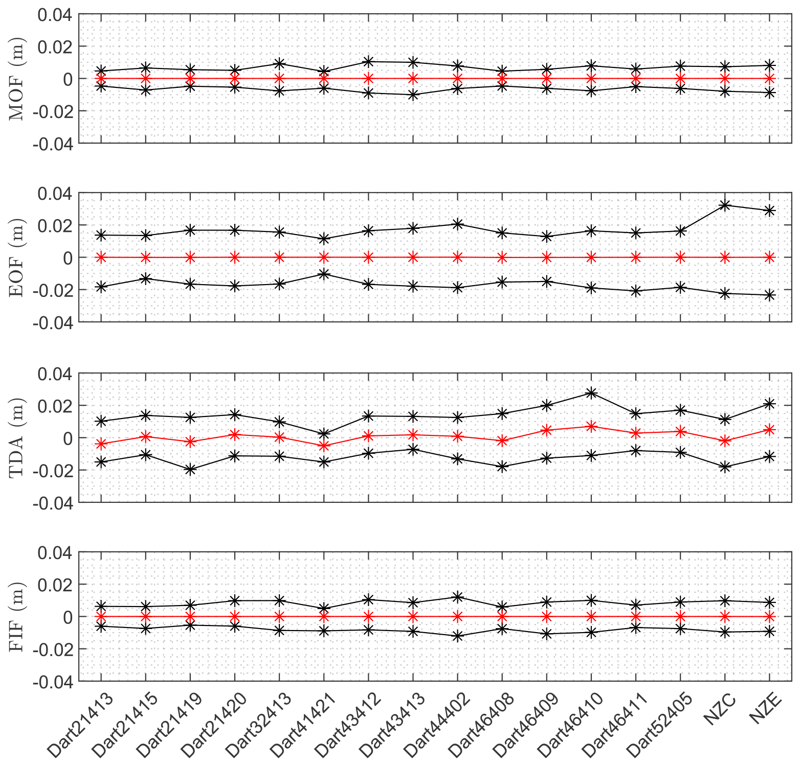
Figure 7 Signal average (red) and maximum and minimum amplitude (black) recorded in each detection curve for all signals in the simultaneous background test. The detection curves have been computed for each of the 16 DART stations reported on the x axis over the period 8–27 April 2021. Note that MOF and FIF have a narrower and more symmetric distribution than EOF and TDA. TDA shows significant asymmetries.

From a spectral point of view, each technique shows consistent results across different instruments. In Fig. 8, we plot the absolute value of the Fourier transform. For each technique, we also plot the average spectra across the different DART stations. All four techniques show consistent frequency peaks, with MOF and FIF showing peaks around the 12 h periods corresponding to the semidiurnal tide period range. EOF has strong peaks for periods of 24, 8, 6 and 4.8 h, corresponding to tidal oscillations not well modeled by the EOF basis. On the other hand, the peak at 12 h is weaker than for the other techniques. Lastly, TDA has strong peaks at diurnal and semidiurnal periods, meaning that the harmonic fit does not capture the entirety of the main tidal oscillations. Furthermore, it is the only technique with significant amplitude at the zero frequency limit, showing the presence of signal-long trends that are not eliminated by either the tide forecast or the bandpass filter.

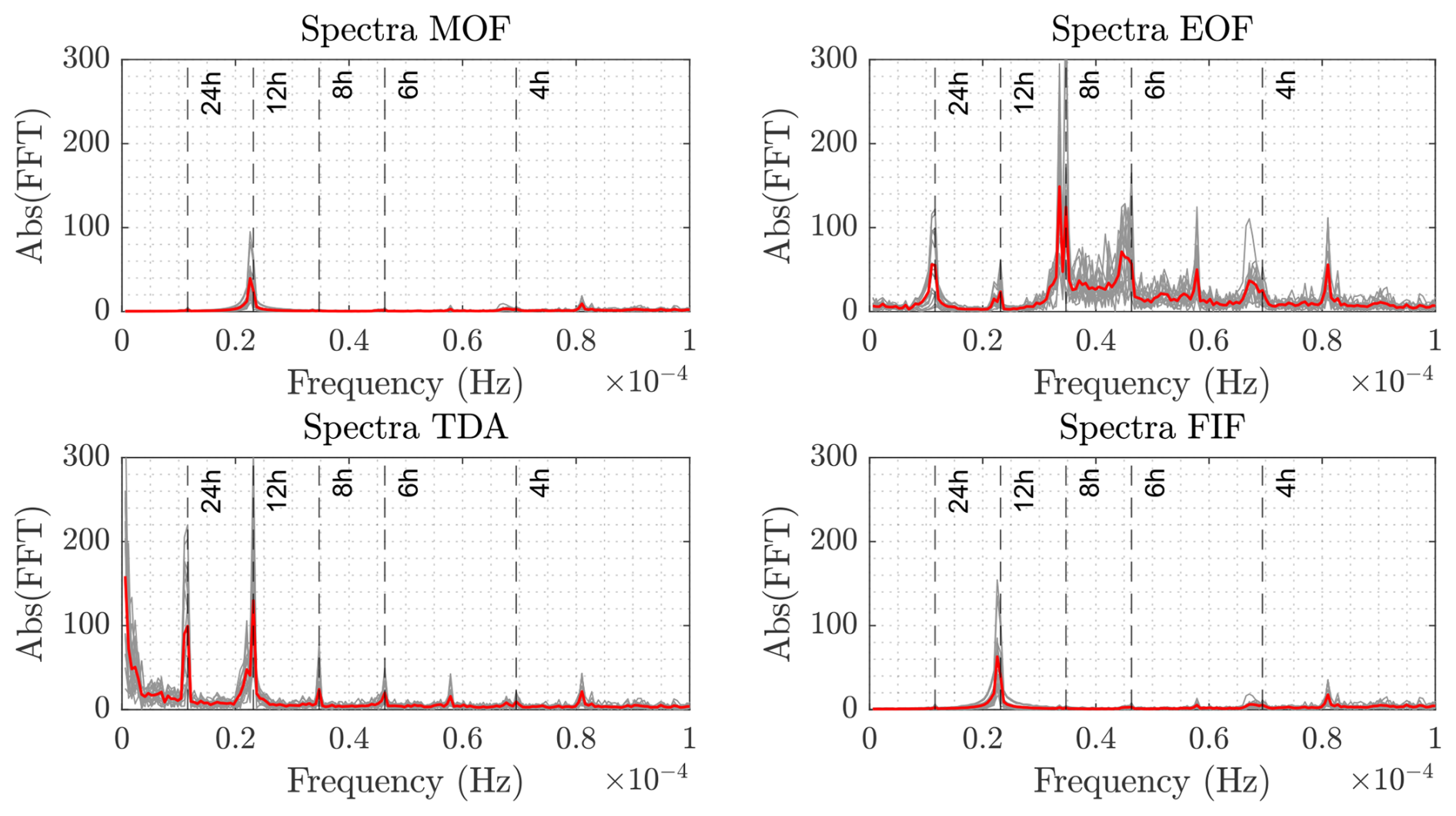
Figure 8 Absolute value of the FFT of each detection curve (gray) and average absolute value of the FFT per technique (red). The detection curves have been computed for each of the 16 DART stations reported on the x axis of Fig. 7 over the period 8–27 April 2021. Note that MOF and FIF show the weakest spectral peak, around the period of semidiurnal tides. EOF and TDA have more pronounced spectral peaks in correspondence of various periods. Signal-long trends in TDA are evident from the larger values in the zero frequency limit.

3.2 Computational cost

Since the main application of a tsunami detection algorithm is in an early warning context, we require the computational time to be low (Beltrami, 2008, 2011). The techniques presented in this work are all applied every time the instrument acquires a new measurement; thus the computational costs for the application to one step must be lower than the acquisition sampling time, which for the DART stations we considered in this study is 15 s. Another common characteristic of these techniques is that each should take a constant time per step, since it performs the same operations in each step. Thus, we can characterize the computational cost of each detection algorithm by computing the time per step.

To this aim, we computed the time each technique takes to compute the first 5000 data points of the detection curves for the background signal A (Fig. 3), reported in Table 3. In all cases, we took into account only computations that are needed in real time while ignoring every computation that may be performed offline, such as the computation of the basis functions for EOF or the tidal coefficients for TDA. Computations have been carried out on an Intel Core i9−11900 CPU, 2.50 GHz, 32.0 GB RAM, Windows 11 Pro computer and with MATLAB R2024a.

Table 3 Total computational time and time per step in seconds required for each technique to compute the first 5000 points of the detection curves in Fig. 4

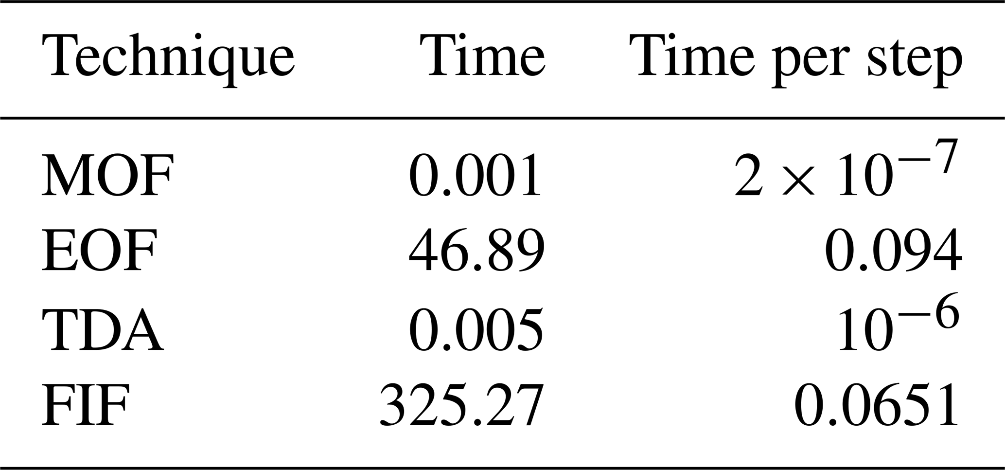
For all techniques the computational time per step is much smaller than the sampling time. Thus, they may all be used for real-time tsunami detection as currently implemented. However, further considerations are needed for real-world applicability. We note that MOF and TDA require less time by orders of magnitude than the other techniques. MOF includes just a few tens of floating-point operations, for which modern hardware is highly optimized. The same is true for TDA, where the computationally heaviest operation, i.e., the fitting procedure to determine tidal coefficients, is carried out offline. On the other hand, EOF detiding and the FIF-based detection technique need 3 to 4 orders of magnitude more computing time. While they are still fast enough to be used for real-time tsunami detection, their applicability to instruments with an autonomous power supply, e.g., DART stations, can be limited by the comparatively larger computational cost.

In regards to the FIF-based detection method, we should also point out that its current implementation described in Sect. 2.4 could be optimized. In fact, we note that a complete decomposition of the signal is computed at each time step. However, the computation could be stopped once the first component with a frequency below the chosen frequency band is extracted. Moreover, the parameters of both the FIF decomposition and the IMFogram algorithm have not been optimized for computational costs. Lastly, the detrending step, carried out with a polynomial fit, might be carried out through more numerically efficient techniques, such as smoothing FIR filters (Schafer, 2011).

3.3 Detection testing on past events

To test how the various algorithms compare in the detection of real events, a dataset based on the catalog by Davies (2019) has been built. The catalog includes 18 events that occurred around the Pacific Ocean between 2006 and 2016, generated by earthquakes with magnitudes between 7.8 and 9.1. For each event, we extracted 24 h long signals starting from the earthquake origin time from every DART station active at origin time whose data are available on NOAA's website. It may happen that data may not be retrieved from some instruments. In these cases, only data transmitted in real time by the instrument are available. For the DART stations concerned here, the raw data's sampling time is 15 s, while it varies for transmitted data between 15 min for normal conditions and 15 s and 1 min for the 4 h after a detection is triggered (Rabinovich and Eblé, 2015). For this reason, the cases where only transmitted data are available have been excluded. Finally, we removed instrumental spikes and resampled by linear interpolation. The dataset obtained contains 437 signals of various nature: some of them consist of only background, while others also contain seismic and/or tsunami waves.

A first comparison between the different techniques can be made by computing the average and standard deviation of each detection curve. The comparison among absolute values of the averages (Fig. 9) gives results similar to the analysis of backgrounds in the previous section: MOF usually produces the smallest residuals followed by FIF, EOF and at last TDA. TDA has worse performance than before due to the variable availability of preceding data, as explained in Sect. 2.3. Thus, TDA was not applicable to 55 signals whose deployment was too recent to compute tidal coefficients, and it shows large residuals if the coefficients were computed from relatively short series.

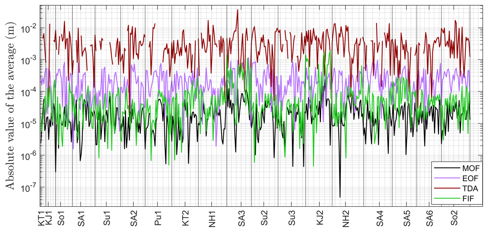
Figure 9 Absolute average value of detection curves for each of the 437 signals in the dataset built by including signals for each event in the catalog by Davies (2019) from every active DART station whose raw data are available through NOAA's Unassessed Ocean Bottom Pressure (highest available resolution) catalog. Detection curves are obtained by applying each of the four techniques to every signal in the dataset. The events to which the signals corresponds are reported along the x axis in chronological order using the nomenclature by Davies (2019). Missing values in the case of TDA corresponds to signals for which there are not enough data for the tidal fit to converge.

Standard deviations are correlated with the total area between the curve and horizontal axis; i.e., we expect the standard deviation to be proportional to the amplitude of oscillations in a signal. Thus, the standard deviations of detection curves with low-amplitude seismic and tsunami components behave similarly to curve averages, as shown in Fig. 10. In contrast, for signals with high-amplitude seismic and/or tsunami components, the various techniques tend to provide similar results. This is evident for the case of the two Kuril Islands events and the Maule event (KJ1, KJ2 and SA3, respectively, in the plot; see Davies, 2019).

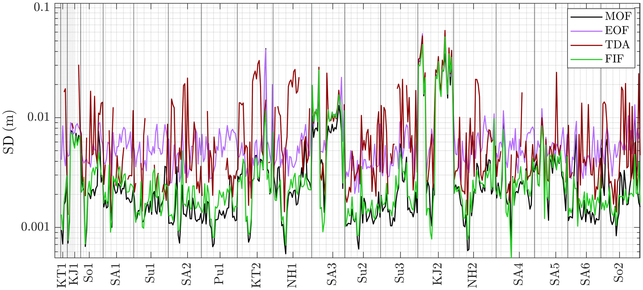
Figure 10 Standard deviation value of detection curves for each of the 437 signals in the dataset built by including signals for each event in the catalog by Davies (2019) from every active DART station whose raw data are available through NOAA's Unassessed Ocean Bottom Pressure (highest available resolution) catalog. Detection curves are obtained by applying each of the four techniques to every signal in the dataset. The events to which the signals corresponds are reported along the x axis in chronological order using the nomenclature by Davies (2019). Missing values in the case of TDA corresponds to signals for which there are not enough data for the tidal fit to converge.

To compare the four techniques, we now try to discriminate false detections and detections triggered by seismic shaking or the tsunami wave. We define the following for a given detection threshold T:

• N – the total number of signals in the dataset;

• n_F – the number of signals with at least one false detection;

• n_E – number of signals with no false detection and at least one earthquake detection;

• n_T – number of signals with no false detection and at least one tsunami detection;

• detection score 1 – ${\mathit{\theta }}_{\mathrm{1}}=\frac{n_{\mathrm{T}}-n_{\mathrm{F}}}{N}$;

• detection score 2 – ${\mathit{\theta }}_{\mathrm{2}}=\frac{n_{\mathrm{T}}-n_{\mathrm{E}}-n_{\mathrm{F}}}{N}$.

These parameters have been computed for each threshold from T = 1.0 cm to T = 4.0 cm with a step of 0.5 cm. We note that the process of attributing a detection to the seismic or tsunami wave trains has been carried out by visual inspection. To avoid possible biases, two strategies are employed. First, the attribution has been as conservative as possible; i.e., any doubtful detection is considered a false detection. Second, we compared detection curves with postprocessed waveforms made available by Davies (2019). To obtain these waveforms, Davies (2019) uses a LOESS smoother to find tides, while seismic waves are removed by truncating the time series. The signals in the dataset for which these are available are 73. Furthermore, the analysis has been applied separately to the set of signals for which we have postprocessed waveforms, which we refer to as the “restricted dataset” and the full dataset.

The differences among techniques may be highlighted by comparing the number of false detections and the detection scores, reported in Fig. 11 as functions of the detection threshold. The number of false detections decreases monotonically with the detection threshold, as we expect. MOF and FIF both have zero false detections above a given threshold, namely 2.5 cm for the full dataset and 2.0 cm for the restricted one. In contrast, EOF and TDA have false detections for each threshold among the ones considered. It is interesting to notice that both reach an asymptote in the restricted dataset for thresholds bigger than or equal to 3.0 cm. This is also the case in the full dataset for EOF but not for TDA. The reason is that the full dataset contains a higher percentage of signals with larger tidal residual, which have an amplitude of several centimeters.

Figure 11 Normalized false detections $n_{\mathrm{F}}/N$ and detections scores θ₁ and θ₂ for each detection technique for the full dataset (left column) and the restricted dataset (right column) of time series available in Davies (2019).

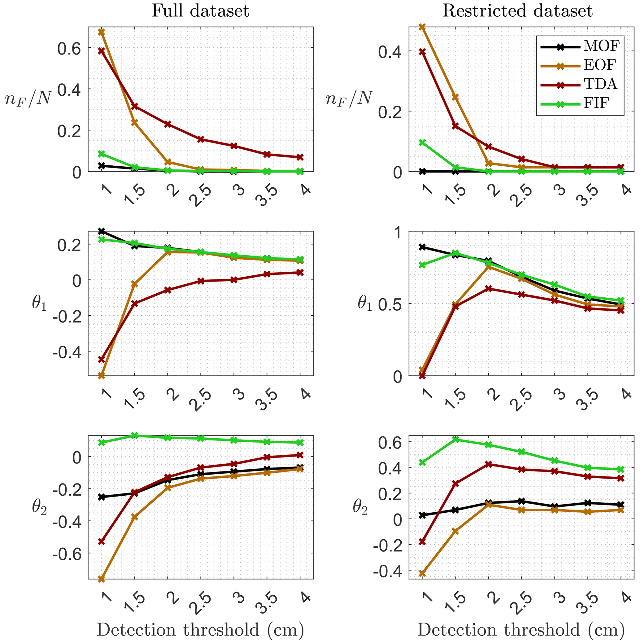
The behavior is different in the case of the θ₁ and θ₂ scores. For θ₁, which can be interpreted as a measure of successful tsunami detections relative to the number of signals with false detections, we observe that MOF always gets better with lower thresholds. On the other hand, for EOF θ₁ has a maximum for a threshold of 2.0 cm. This can be interpreted as the optimal threshold for EOF if θ₁ is assumed to be a good performance metric. TDA and FIF show a slightly different behavior between the two datasets. FIF has an optimal threshold T = 1.5 cm for the restricted dataset. TDA has the same optimum T = 2.0 cm as EOF for the restricted dataset, while in the full dataset the presence of signals with large residuals dominates as in the previous case.

θ₂ is similar to θ₁, with the added goal of minimizing the number of earthquake detections. In the restricted dataset, MOF and EOF perform worse than TDA and FIF, since the latter two filter out the high-frequency content. Exactly as it happens for θ₁, EOF and TDA reach optimal score values at T = 2.0 cm and FIF does at T = 1.5 cm. However, in the full dataset FIF is the only technique with an optimal threshold, again equal to 1.5 cm. For the other techniques, θ₂ increases monotonically with the detection threshold. While for TDA the reason is the same as before, MOF's and EOF's performance is dominated by the larger amount of recorded seismic waves.

3.4 Waveform characterization in FIF-based detection

According to Beltrami (2008), one of the desirable properties of a tsunami detection algorithm is the correct characterization of the wave in terms of amplitude and period. While these properties have already been investigated for MOF (Beltrami, 2011), EOF (Tolkova, 2009, 2010) and TDA (Chierici et al., 2017), they have yet to be established in the case of FIF. In particular, we are interested in determining

1. the behavior of signals where no earthquake or tsunami is present,

2. how seismic waves are filtered and the separation between Rayleigh waves and tsunami waves in the near field,

3. if we can determine the correct tsunami waveform from the detection algorithm.

Regarding point 1, detection curves generally behave as expected from the analysis of the background signal (see Sect. 3.1), with amplitudes mostly within 1.0 cm and no strong residual oscillation.

For point 2, we already pointed out in Sect. 3.3 that FIF filtering capabilities are well illustrated by the variation in θ₂ as a function of the detection threshold. However, even when the earthquake is detected, FIF allows seismic and tsunami waves to be better separated. This is exemplified in Fig. 12, showing the application of the techniques to DART 51425 recorded during the 29 September 2009 Samoa earthquake and tsunami. In this case, all four techniques would register a detection at the passage of seismic waves, but the corresponding amplitude varies a lot between MOF and EOF (∼ 85 cm, not shown in the figure) and TDA and FIF (∼ 10 cm). Furthermore, while for the first two the seismic wave train overlaps with the tsunami wave, for the last two there is a clear separation, allowing for a better estimation of the tsunami amplitude, which represents an important observable that is part of a tsunami alert statement.

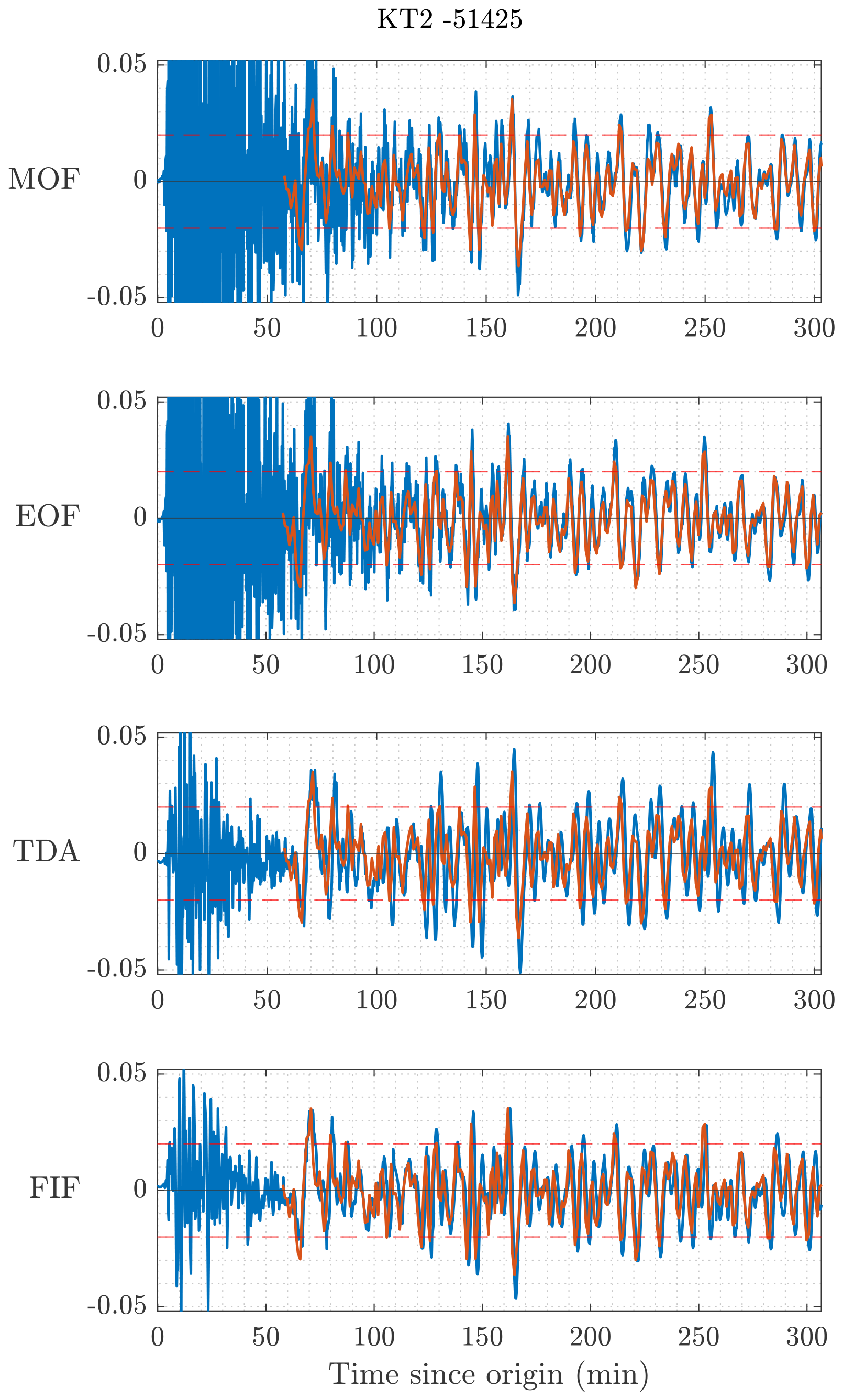
Figure 12 Comparison of detection curves (in blue) and postprocessed tsunami waveforms (orange) for the 29 September 2009 Samoa tsunami as recorded by DART 51425. Dashed, horizontal red lines are located at ±2 cm.

In the analysis, we found a limited number of signals where FIF detection curves present jump discontinuities during the tsunami passage in cases where the signal is very steep. Since the occurrence of these discontinuities only happens during a tsunami, they do not hinder in any way the detection capabilities of the technique. However, such cases may be problematic in data assimilation applications, where the full waveform is needed. In these cases, we can use the tsunami component produced by the decomposition (step 4 in the procedure described in Sect. 2.4) at the time of assimilation.

As shown in Fig. 13, the tsunami components extracted during monitoring at different times approximate the tsunami waveform much better than the detection curve by itself. However, the use of the full component extracted through FIF decomposition may be a heavy operation to perform in real time, since it would require the transmission of a 3 h long signal, i.e., a 720-element-long vector, instead of a single number as needed for the detection curves. In instruments where power management is critical, such as DART stations, this operation should be performed rarely, e.g., once at a fixed time after detection, if precise data are needed, as is the case in data assimilation contexts (Wang et al., 2019b). Lastly, we also note that such large discontinuities in the detection curve are present in very few detection curves and that the example in Fig. 13 is the most pathological.

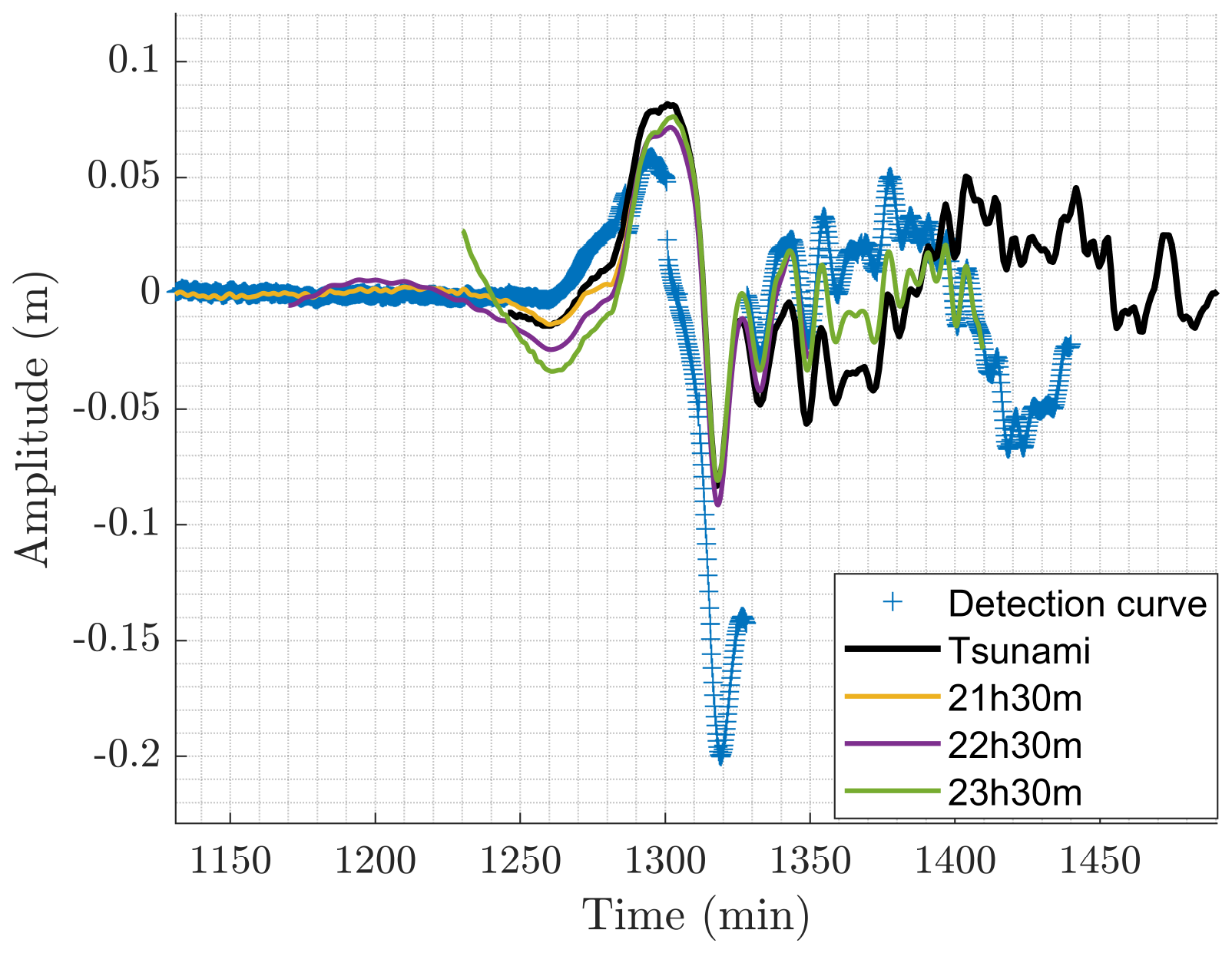
Figure 13 Example of the tsunami components (yellow, purple and green curves) extracted during monitoring compared with the postprocessed waveform (black) and the detection curve (blue crosses) obtained with the FIF-based technique. Time is measured from the earthquake origin time. Data from the record at DART 21413 for the 2010 Maule tsunami.

4 Conclusions

Four tsunami real-time detection algorithms, one of which is presented in this work for the first time, have been analyzed and compared. In particular, they have been tested against a large amount of real OBPG data from NOAA's and GeoNet's DART networks, both in the presence and in the absence of oscillations related to the earthquake and the tsunami. Firstly, we have determined the main properties of the techniques by analyzing their application to background signals. These background tests, which include five signals of 1-month duration and signals of 20 d duration acquired simultaneously from 16 different stations, show consistent results in terms of amplitude and spectral content. After that, a dataset of tsunami signals from past events has been analyzed and detection rates of each technique have been quantified through simple detection scores, with the goal of determining optimal detection thresholds.

For detection applications only, Mofjeld's algorithm remains the best-performing technique, both in terms of detection metrics and computational speed. However, the algorithm is not the most suitable to correctly characterize the tsunami waves or to filter out high-frequency components (e.g., the seismic Rayleigh waves). The EOF and TDA techniques present variable behavior. EOF is not able to reduce the tidal residual below ∼ 2 cm, leading to incorrect characterization of low-amplitude tsunami signals. TDA has a strong dependence on the precision of precomputed tidal coefficients, resulting in a large number of detection curves with amplitudes of several centimeters, too large for a precise detection of offshore-traveling tsunamis. Investigating a combination of TDA with a different detiding technique may be the subject of future work.

The newly developed FIF-based detection method possibly shows the best compromise between detection and real-time characterization. Optimal detection thresholds for the technique have been determined to be

1. T = 2 cm for the goal of minimizing false detections

2. T = 1.5 cm for maximizing tsunami detection with respect to earthquake and false detections, based on two simple detection scores.

Furthermore, it is shown that the entire tsunami component over the 3 h period reproduces accurately the tsunami waveform, allowing the characterization of wave amplitude and period even in the rare cases where the detection curves fail to do so.

Future work is planned for the application of the technique to the DART 4G stations and non-OBPG data (e.g., coastal tide gauges) and to tsunamis of nonseismic origin, for example for OBPGs which are planned at Stromboli to monitor volcano-induced tsunamis (Selva et al., 2021a). On the other hand, the technique is already fast enough to be applied in real time, but an onboard implementation will require greater optimization to limit power consumption, especially in the case where the entire tsunami components have to be transmitted. Future work is then also planned for the numerical optimization of the technique by exploiting the recent installation of SMART cables (Howe et al., 2019) and also in view of the recent installations in the Ionian Sea of a dedicated instrumented cable to detect earthquakes and tsunamis (Marinaro et al., 2024) and of further DART-like OBPGs by CAT-INGV (Amato et al., 2021).