Adaptive behavior of farmers under consecutive droughts results in more vulnerable farmers: a large-scale agent-based modeling analysis in the Bhima basin, India

Consecutive droughts, becoming more likely, produce impacts beyond the sum of individual events by altering catchment hydrology and influencing farmers' adaptive responses. We use the Geographical, Environmental, and Behavioural (GEB) model, a coupled agent-based hydrological model, and expand it with the subjective expected utility theory (SEUT) to simulate farmer behavior and subsequent hydrological interactions. We apply GEB to analyze the adaptive responses of ∼1.4 million heterogeneous farmers in India's Bhima basin over consecutive droughts and compare scenarios with and without adaptation. In adaptive scenarios, farmers can either do nothing, switch crops, or dig wells, based on each action's expected utility. Our analysis examines how these adaptations affect profits, yields, and groundwater levels, considering, e.g., farm size, risk aversion, and drought perception. Results indicate that farmers' adaptive responses can decrease drought vulnerability and impact after one drought (6 times the yield loss reduction) but increase them over consecutive periods due to switching to water-intensive crops and homogeneous cultivation (+15 % decline in income). Moreover, adaptive patterns, vulnerability, and impacts vary spatiotemporally and between individuals. Lastly, ecological and social shocks can coincide to plummet farmer incomes. We recommend alternative or additional adaptations to wells to mitigate drought impact and emphasize the importance of coupled socio-hydrological agent-based models (ABMs) for risk analysis or policy testing.

1 Introduction

Anthropogenic climate change and population growth have increased the exposure of societies to droughts (Smirnov et al., 2016). Furthermore, the growing demand on water increasingly stresses freshwater systems, amplifying the impact of droughts (Best and Darby, 2020; Van Loon et al., 2016). Therefore, there is a necessity to strive for drought risk adaptation both at larger scales by governments (e.g., reservoir management) and at local scales by farmers through efficient water use and irrigation (UNDRR, 2015; Wilhite et al., 2014).

Empirical research into what factors drive adaptation is ongoing but mostly focuses on single events and at one point in time (Blauhut et al., 2016; Udmale et al., 2015). However, consecutive droughts are becoming more likely and can result in impacts that differ from the sum of the individual events' parts (Anderegg et al., 2020; van der Wiel et al., 2023; Zscheischler et al., 2020). Consecutive droughts impact farmer communities via a few distinct (but interrelated) processes. (1) The first (of consecutive) drought(s) can have a physical hydrological impact on the second drought. For example, a lowered groundwater table after the first event may not have been replenished before the second drought starts, which can limit the capacity for irrigation during the second drought (Anderegg et al., 2020; van der Wiel et al., 2023; Zscheischler et al., 2020). (2) Moreover, socio-economic factors like income or debt also influence the vulnerability of farmers and their ability to adapt during multiple drought events. For example, the reduced income of farmers after a first drought (e.g., due to less yield) may lead to less financial capacity to cope with the second drought. (3) Finally, behavioral factors such as risk aversion and risk perception also play a role in how farmers adapt to (multiple) droughts (Habiba et al., 2012; Ward et al., 2014). For example, farmers can have an increased risk perception after the first event, which may lead to an accelerated implementation of drought adaptation measures (Aerts et al., 2018; van Duinen et al., 2015; Habiba et al., 2012; Nelson et al., 2013), thus reducing the impact of the second drought.

A key research challenge is to capture the spatiotemporal dynamic feedbacks between vulnerability, human behavior, and physical hydrological processes over periods with consecutive droughts (Cui et al., 2021; Trogrlić et al., 2022; van der Wiel et al., 2023). Empirical data from surveys may support analysis about the factors driving drought adaptation feedbacks. However, only a few studies provide empirical data on the spatiotemporal drivers of drought vulnerability and adaptation under multi-drought conditions (Kreibich et al., 2022). This is why current drought risk assessment research suggests developing model-based approaches (Cui et al., 2021; Trogrlić et al., 2022).

A special class of simulation models is called agent-based models (ABMs). ABMs are specially designed to capture the behavior of autonomous individuals (i.e., agents) (Blair and Buytaert, 2016; Schrieks et al., 2021; Wens et al., 2019). When integrated with a hydrological model, they can also capture bi-directional human–water feedbacks, with agents reacting to environmental changes (e.g., precipitation deficits) and impacting their surroundings (e.g., depleting groundwater levels) (de Bruijn et al., 2023; Klassert et al., 2023; Yoon et al., 2021). In contrast to other socio-hydrological models, ABMs can simulate how drought adaptation of individual farmers is influenced by other agents. This is essential, as adaptive feedbacks by farmers are heterogeneous and depend on the varying physical, socio-economic, and behavioral characteristics among the farmer population (e.g., risk aversion, income, farm size, adaptations, upstream/downstream location, proximity to reservoirs; Di Baldassarre et al., 2018; Habiba et al., 2012; Udmale et al., 2014, 2015). For example, government-led large-scale adaptation efforts, like reservoir management, may affect farmers' irrigation usage (Di Baldassarre et al., 2018). Additionally, agents can emulate their neighbors' practices, such as cropping patterns (Baddeley, 2010). However, most ABM-based studies that simulate individual farmers remain at small scales (Zagaria et al., 2021), whereas studies at large basin scales aggregate agents, data, and processes and omit small-scale behavior due to computational constraints (Castilla-Rho et al., 2017; Hyun et al., 2019).

To address these challenges, de Bruijn et al. (2023) developed the Geographic, Environmental, and Behavioural (GEB) model, an ABM coupled with a hydrological model (CWatM, Burek et al., 2020) that is able to model the behavior of millions of agents efficiently at a “one-to-one” scale, meaning for each farmer in the study area, an individual farmer agent is modeled. With GEB, it is possible to analyze the culminated hydrological and agricultural impacts of many small-scale processes at the river basin scale. However, to analyze the complex human decision-making process under consecutive droughts we require a farmer's characteristics and behavior to change dynamically in response to drought events (Groeneveld et al., 2017; Pahuja et al., 2010; Schrieks et al., 2021; Shah, 2009). In the current version of GEB this is not possible, as its decision rules for adaptation are based only on imitating neighbors that currently have higher profits, without accounting for dynamic risk perception, previously incurred debts due to drought loss or adaptation (Solomon and Rao, 2018; Udmale et al., 2014, 2015), the possibility of future droughts, or heterogeneous farmer characteristics such as risk aversion (de Bruijn et al., 2023; Schrieks et al., 2021).

The main goal of this study is to assess the vulnerability and adaptive responses of farmer agents under consecutive droughts. Therefore, we integrate the subjective expected utility theory (SEUT; Savage, 1954; Fishburn, 1981) into the GEB model in combination with imitation (Baddeley, 2010) and elements of prospect theory (Kahneman and Tversky, 2013; Ribeiro Neto et al., 2023). The SEUT is a well-established behavioral economic theory that explains farmer adaptation decisions as economic maximization under risk, influenced by subjective estimates of drought probability and factors such as risk aversion and time-discounting preferences. By parameterizing and calibrating the SEUT with local data and letting the risk perception change dynamically in response to drought events, we attempt to create a more accurate depiction of adaptation under consecutive droughts. We further refine our characterization of farmers – including their drought experience, adaptation costs, and loan debts – to better understand changes in their individual vulnerability and risk, such as fluctuations in income, debt levels, adaptation uptake, and groundwater levels.

We apply and calibrate the augmented GEB in the Bhima basin, which is part of the Krishna basin in India. Our work helps in understanding how consecutive drought events affect different types of farmers' vulnerability and impact. The paper is organized as follows: we begin with a high-level overview of the model setup (Sect. 2.1) and a description of the study area (Sect. 2.2). We then detail our implementation of behavior (Sect. 2.3), crop cultivation methods (Sect. 2.4), and agent initialization (Sect. 2.5) and conclude with model calibration and a scenario setup (Sect. 2.6). Next, in the Results section, we analyze the evolution of model vulnerability and risk parameters over consecutive droughts in an adaptation scenario (Sect. 3.1) and compare it to a no-adaptation scenario (Sect. 3.2). This leads into a discussion of our key findings and challenges to our methods (Sect. 4). Finally, we summarize our conclusions and suggest directions for future research (Sect. 5).

2 Methods

2.1 Model setup

Figure 1 shows the structure of the GEB model. GEB is developed in Python and couples a large-scale agent-based model (orange part) that simulates the adaptation behavior of millions of agents (farmers and reservoir operators) (de Bruijn et al., 2023) to a hydrological model (blue part) simulated with the CWatM (Burek et al., 2020) and MODFLOW models (Langevin et al., 2017). The hydrological processes of CWatM operate at daily time steps at a 30 arcsec grid size, while GEB's agent processes are at the sub-grid level. The interactions between both, such as irrigation, occurs daily, while adaptation decisions are made at the end of each growing season for the next one. The CHELSA-W5E5 v1.0 observational climate input data at 30 arcsec horizontal and daily temporal resolution were used as climate forcing (Karger et al., 2022). We do not aggregate agents; thus for approximately each farmer in the river basin we generate one representative agent, which we refer to as the one-to-one scale. The agent's individual characteristics are derived from socio-economic data (census data on, e.g., income), survey data (on, e.g., risk aversion, discount rate), agricultural data (past yields, crop rotations, farm sizes), and data on the past climate and droughts (SPEI, standardized precipitation evapotranspiration index) (Sect. 2.3–2.5). These data are used to calculate the subjective expected utility (SEUT) equation to determine whether a farmer adapts or not, given the hydroclimatic context. For an extensive model overview, see the ODD+D protocol (Sect. S1 in the Supplement; Müller et al., 2013).

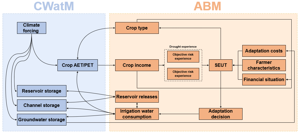
Figure 1 Simplified setup integrating the hydrological model CWatM (blue boxes) with an agent-based model (orange boxes). AET: actual evapotranspiration, PET: potential evapotranspiration.

2.2 Case study

The upper Bhima catchment in Maharashtra, spanning 45 678 km², varies in elevation from 414 m in the east to 1458 m in the Western Ghats mountain range (Fig. 2). The catchment is mostly flat, with 95 % of its area below 800 m. The area experiences significant rainfall variation due to interaction of the monsoon and the Western Ghats, ranging from 5000 mm in the mountains to less than 500 mm in the east (Gunnell, 1997). Over 90 % of this rain falls during the monsoon months (June–September), with substantial deficits from October to May. The state's agricultural cycle includes the monsoon kharif season (June–September) and the dry rabi season (October–March), with April and May constituting the hot summer period.

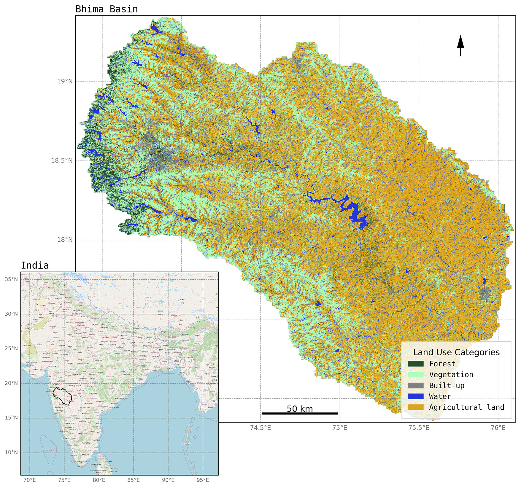
Figure 2 Overview of the Bhima basin's location in India and the land use classification used in the model. The forested area in the west is the Western Ghats mountain range. Map of the Bhima basin land cover produced from land cover data from Jun et al. (2014). © OpenStreetMap contributors 2024. Distributed under the Open Data Commons Open Database License (ODbL) v1.0.

To manage the water supply, reservoirs in the Western Ghats accumulate water during monsoon rains. This water is released to the river and to farmers in the reservoir through areas with a system of canals during the monsoon (kharif) and the dry irrigation season (rabi and summer). This results in human-controlled river flows, which are less dependent on natural climate patterns (Immerzeel et al., 2008). Although reservoirs distribute irrigation water, agriculture in Maharashtra still mainly relies on monsoon rain, with 19.7 % of the state's gross cropped area being irrigated and 80.2 % being dependent on rainfed farming (Udmale et al., 2015). During the study period there were approximately three periods with a prolonged negative 12-month standardized precipitation evapotranspiration index (SPEI) score: a severe (−1.5 to −1.99 SPEI, 2000–2005), a mild (0 to −0.99 SPEI, mid-2009 to 2010), and a final moderate (−1.0 to −1.49 SPEI, mid-2012 to 2015) drought (Fig. 3; McKee et al., 1993). During the last drought there was a brief period of positive SPEI, but for ease of referencing we refer to it as one drought.

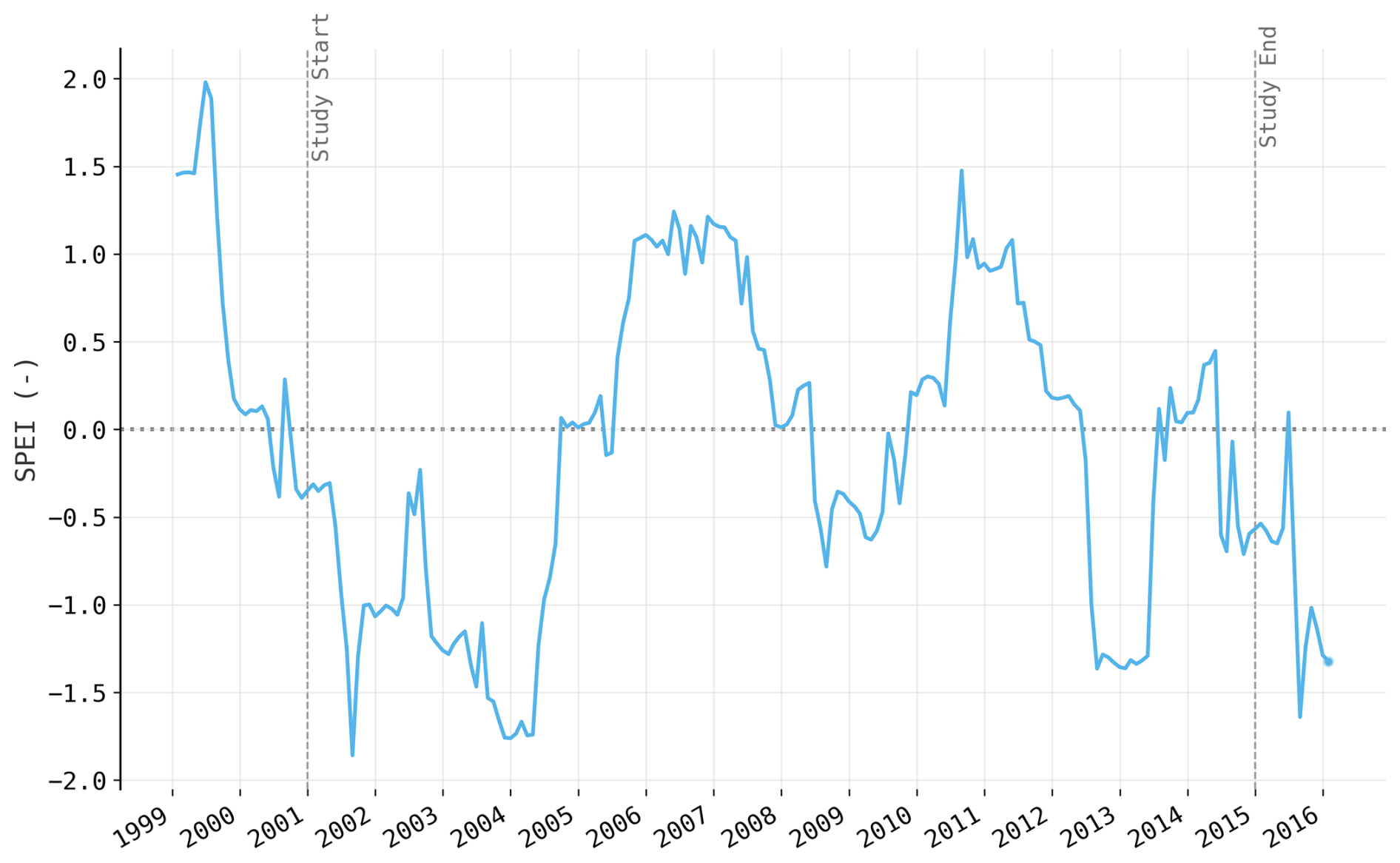
Figure 3 The average 12-month standardized precipitation evaporation index (SPEI) in the Bhima basin. Derived from the CHELSA-W5E5 v1.0 dataset (Karger et al., 2022).

2.3 Farmer decision rules

Agents base their decisions on the SEUT (Fishburn, 1981; Savage, 1954) in combination with imitation of their neighbors (Baddeley, 2010; Haer et al., 2016) and elements of prospect theory (Kahneman and Tversky, 2013; Ribeiro Neto et al., 2023). The SEUT builds on the EUT (Von Neumann and Morgenstern, 2007) by incorporating the concept of “bounded rationality”, where agents remain rational utility maximizers but base their decisions on subjective estimates of drought probability. Their subjective estimates overestimate probabilities following a drought and underestimate probabilities after periods of no drought. Such boundedly rational behavior, observed in reality (Aerts et al., 2018; Kunreuther et al., 1985), aligns more closely with actual adaptation behavior than fully rational models (Haer et al., 2020; Wens et al., 2020) and has been incorporated into various ABMs to simulate adaptive behavior (Groeneveld et al., 2017; Haer et al., 2020; Tierolf et al., 2023; Wens et al., 2020). Furthermore, the SEUT also accounts for an individual's subjective characteristics (i.e., risk aversion and discount rate). At each yearly time step agents calculate the following (S)EUTs:

1. SEUT of taking no action (Eq. 1)

2. SEUT of investing in a (tube) well (Eq. 2)

3. SEUT of their current crop rotation (Eq. 3)

4. EUT of their current crop rotation (Eq. 4).

2.3.1 Crop switching

To switch crops, farmers imitate their most successful neighbor. This is done for two reasons: first, literature shows that people tend to emulate their neighbors' practices (Baddeley, 2010; Haer et al., 2016). Second, there are over 300 unique crop rotations used within the model. The expected utility calculation (GEB) is optimized for handling many agents simultaneously but is not designed for frequent repetition. Thus, it would be computationally inefficient for each agent to calculate the SEUT for each rotation. Therefore, all agents calculate only their own crop rotation's SEUT (Eq. 3) and EUT (Eq. 4; using neutral risk perception, aversion, and the discount rate; Sect. 2.5). Then, agents compare their current crop rotation's SEUT with the EUT of a random selection of a maximum of five random neighboring farmers using similar irrigation sources (within a 1 km radius, using a reservoir, surface water, groundwater, or no irrigation). The EUT is used since using a neighbor's SEUT would mean using another agent's subjective factors. They then adopt the crop rotation of the neighbor whose EUT is highest if this exceeds their own SEUT.

2.3.2 Well adaptation

To decide whether to invest in a well, agents compare the SEUT of taking no action (Eq. 1) with the SEUT of digging a well (Eq. 2). When the SEUT favors adaptation and adapting is within the agent's budget constraints, the farmers invest in a well.

$$\begin{array}{}\text{(1)}& {\displaystyle }{\mathrm{SEUT}}_{\mathrm{no}\mathrm{\_}\mathrm{action}}=\underset{p_{\mathrm{2}}}{\overset{p_{\mathrm{1}}}{\int }}{\mathit{\beta }}_{t,x}\cdot p_i\cdot U\left(\sum _{t=\mathrm{0}}^T{\displaystyle \frac{{\mathrm{Inc}}_{i,x,t}}{{\left(\mathrm{1}+r_x\right)}^t}}\right)\mathrm{d}p\text{(2)}& {\displaystyle }{\mathrm{SEUT}}_{\mathrm{tube}\mathrm{\_}\mathrm{well}}=\underset{p_{\mathrm{2}}}{\overset{p_{\mathrm{1}}}{\int }}{\mathit{\beta }}_{t,x}\cdot p_i\cdot U\left(\sum _{t=\mathrm{0}}^T{\displaystyle \frac{{\mathrm{Inc}}_{i,x,t}^{\mathrm{well}}-C_{t,x,\mathrm{d}}^{\mathrm{well}}}{{\left(\mathrm{1}+r_x\right)}^t}}\right)\mathrm{d}p\text{(3)}& {\displaystyle }{\mathrm{SEUT}}_{\mathrm{own}\mathrm{\_}\mathrm{crop}\mathrm{\_}\mathrm{rotation}}=\underset{p_{\mathrm{2}}}{\overset{p_{\mathrm{1}}}{\int }}{\mathit{\beta }}_{t,x}\cdot p_i\cdot U\left(\sum _{t=\mathrm{0}}^T{\displaystyle \frac{{\mathrm{Inc}}_{i,x,t}-C_{t,x,\mathrm{c}}^{\mathrm{input}}}{{\left(\mathrm{1}+r_x\right)}^t}}\right)\mathrm{d}p\text{(4)}& {\displaystyle }{\mathrm{SEUT}}_{\mathrm{own}\mathrm{\_}\mathrm{crop}\mathrm{\_}\mathrm{rotation}}=\underset{p_{\mathrm{2}}}{\overset{p_{\mathrm{1}}}{\int }}{p}_i\cdot U\left(\sum _{t=\mathrm{0}}^T{\displaystyle \frac{{\mathrm{Inc}}_{i,x,t}-C_{t,x,\mathrm{c}}^{\mathrm{input}}}{{\left(\mathrm{1}+r_x\right)}^t}}\right)\mathrm{d}p\end{array}$$

Utility U(x) is a function of expected income Inc and potential-adapted income Inc^well per event i and adaptation costs C^well for each agent x. In Eq. (2), C^well is dependent on groundwater levels d, and C^input in Eq. (4) is dependent on current market prices for the crops c that the agent x is currently cultivating. To calculate the utility of all decisions, we take the integral of the summed time-discounted utility, with the discount factor r and time (t) in years, under all possible events i with a probability of p_i and adjust p_i with the subjective risk perception β_t for each agent x. See Sect. S1.2.2 for an overview of all model parameters.

2.3.3 Predicted income

To calculate the expected utility, we need information on farmer income during droughts of varying return periods with and without an adaptation. Since droughts of similar return periods have different severities depending on the farmer's location and since this relation is also dependent on each farmer's crop rotation and irrigation capabilities, no straightforward empirical relationship exists. Therefore, we established this relationship endogenously for each farmer in the following manner. After each harvest, the 12-month SPEI (derived from the CHELSA climate data between 1979 and 2016) at the time of harvest and the harvest's yield ratio (Sect. 2.4) are determined for each agent. The SPEI is converted to a drought probability, and these values are then averaged per year. In order to get more data points, they are then averaged per farmer group, which are based on farmers' elevation (upstream, midstream, downstream), irrigation (well or no well), and crop rotation. Then, a relation (Eq. 5) is fitted between drought probability and yield ratio for each group using the last 20 years of data (a spin-up period of 20 years is used where no behavior occurs). We refer to this relation as the agent's objective drought risk experience. The 12-month SPEI and base-2 logarithm were chosen as they returned the highest R² between drought probability and yield ratio for this region (∼0.50).

$$\begin{array}{}\text{(5)}& {\mathrm{SPEI}}_{i,t}=a\cdot {\log }_{\mathrm{2}}\left({\mathrm{yield}}_{i,t}\right)+b\end{array}$$

The relation between probability and the yield ratio is used to derive yield ratios associated with 1-, 2-, 5-, 10-, 25-, and 50-year return period drought events i, which are then converted to income per return period event Inc_i (Sect. 2.4). To determine their potential income after adaptation Inc^adapt, within groups of similar cropping and elevation, the non-irrigating groups determine their yield ratio gain from the yield ratios of their well-irrigating counterparts.

2.3.4 Cost of wells

To determine the cost of wells, we adapted the cost equations and parameterization of Robert et al. (2018) (Sect. S3.4.1). These are a function of pump horsepower, pumping hours, electricity costs, the probability of well failure, maintenance costs, and drilling costs. Drilling costs are dynamic and dependent on the well's depth, which are put at 20 m below the current groundwater table. Together with the agent's interest rate r (Sects. 2.4 and S2.1.4), this is converted to an annual implementation cost C^adapt for the n-year loan using Eq. (6).

$$\begin{array}{}\text{(6)}& C_{t,\mathrm{d}}^{\mathrm{adapt}}=C_{\mathrm{d}}^{\mathrm{fixed}\mathrm{cost}}\cdot {\displaystyle \frac{r\cdot (\mathrm{1}+r{)}^n}{(\mathrm{1}+r{)}^n-\mathrm{1}}}+C_t^{\mathrm{yearly}\mathrm{costs}}\end{array}$$

2.3.5 Crop cultivation costs

Yearly cultivation input costs C^input per hectare for each crop type c, which include expenses such as purchasing seeds, manure, and labor, are sourced from the Ministry of Agriculture and Farmers Welfare in rupees (INR) per hectare (https://desagri.gov.in/document-report-category/cost-of-cultivation-production-estimates/, last access: 20 February 2025) (de Bruijn et al., 2023).

2.3.6 Loans and budget constraints

We assume that agents are “saving down” (Bauer et al., 2012) and taking loans for agricultural inputs (Hoda and Terway, 2015) and investments using Eq. (6). We assume farmers cannot spend their full income on inputs and investments and implement an expenditure cap (Hudson, 2018), which we use as a calibration factor (Sect. 2.6). If the proposed annual loan payment for a well exceeds the expenditure cap, agents are unable to adapt. Chand et al. (2015) put the expenditure of inputs such as seeds, fertilizer, plant protection, repair, and maintenance feed and other inputs at approximately 20 %–25 %. Thus, including the extra well investment cost, we calibrate the expenditure cap of yearly payments to between 20 %–50 % of yearly non-drought income (Pandey et al., 2024).

2.3.7 Time discounting and risk aversion

For Eqs. (1)–(3) the agent's individual discount rate and risk aversion (Sect. 2.5) are used. For Eq. (4), as the goal is a “neutral” expected utility of a farmer's crops, all farmers use the average discount rate and risk aversion. For Eqs. (1) and (2) a time horizon of 30 years following Robert et al. (2018) is used, while for Eqs. (3) and (4) a time horizon of 3 years is used. The utility U(x) as a function of risk aversion σ is as follows:

$$\begin{array}{}\text{(7)}& U\left(x\right)={\displaystyle \frac{x^{\mathrm{1}-\mathit{\sigma }}}{\mathrm{1}-\mathit{\sigma }}}.\end{array}$$

2.3.8 Bounded rationality

Bounded rationality within the SEUT is described by the risk perception factor β. β rises after agents have experienced a drought, overestimating drought risk (β>1). After time without a drought, it lowers again, underestimating risk (β<1). We follow the setup of Haer et al. (2020) and Tierolf et al. (2023) and define β as a function of t years after a drought event:

$$\begin{array}{}\text{(8)}& {\mathit{\beta }}_t=c\cdot {\mathrm{1.6}}^{-d\cdot t}+e.\end{array}$$

We set d to −2.5, resulting in a slower risk reduction than in Haer et al. (2020) and Tierolf et al. (2023), as farmers are assumed to retain more awareness of drought risk compared to households of flood risk (van Duinen et al., 2015). We set the minimum underestimation of risk e to 0.01 and calibrate the maximum overestimation of risk c between 2 and 10 (Botzen and van den Bergh, 2009).

2.3.9 Drought loss threshold

As the onsets of droughts are not as obvious as with floods (Van Loon et al., 2016), we define an agent's drought event perception (Bubeck et al., 2012) according to a loss in the yield ratio against a moving reference point, similar to prospect theory (Kahneman and Tversky, 2013; Ribeiro Neto et al., 2023). The moving reference point is the 5-year average difference between the reference potential yield and the actual yield (Sect. 2.4). We calibrate the drought loss threshold between 5 % and 25 %. This means that if the current harvest's difference between the potential and actual yield falls 5 %–25 % below the historical average, the years since the last drought event t (Eq. 8) are reset and β rises.

2.3.10 Microcredit

If the yield falls below the drought loss threshold, agents will also take out a loan equal to the missed income (Udmale et al., 2015). The loan duration is set to 2 years (Rosenberg et al., 2013).

2.4 Farmer crop cultivation

2.4.1 Yield and income

Farmers grow pearl millet (bajra), groundnut, sorghum, paddy, sugar cane, wheat, cotton, chickpea, maize, green gram, finger millet, sunflower, and red gram. Each crop undergoes four growth stages (d₁ to d₄). The crop coefficient (K_c) for a particular day is then calculated as follows (Fischer et al., 2021):

$$\begin{array}{}\text{(9)}& \begin{array}{rl}& K_{{\mathrm{c}}_t}=\\ & \left\{\begin{array}{ll}{K}_{{\mathrm{c}}_{\mathrm{1}}},& t<d_{\mathrm{1}}\\ K_{{\mathrm{c}}_{\mathrm{1}}}+\left(t-d_{\mathrm{1}}\right)\times \frac{K_{{\mathrm{c}}_{\mathrm{2}}}-K_{{\mathrm{c}}_{\mathrm{1}}}}{d_{\mathrm{2}}},& d_{\mathrm{1}}\le t<d_{\mathrm{2}}\\ K_{{\mathrm{c}}_{\mathrm{2}}}& d_{\mathrm{2}}\le t<d_{\mathrm{3}}\\ K_{{\mathrm{c}}_{\mathrm{2}}}+\left(t-\left(d_{\mathrm{1}}+d_{\mathrm{2}}+d_{\mathrm{3}}\right)\right)\times \frac{K_{{\mathrm{c}}_{\mathrm{3}}}-K_{{\mathrm{c}}_{\mathrm{2}}}}{d_{\mathrm{4}}},& \mathrm{otherwise}\end{array}\right.,\end{array}\end{array}$$

where t represents the number of days since planting and d₁ to d₄ are the crop-specific durations of each growth stage. K_c is multiplied daily with the reference potential evapotranspiration to determine the crop-specific potential evapotranspiration (PET_t). At the harvest stage, the actual yield (Y_a) is determined based on a maximum reference yield (Y_r; Siebert and Döll, 2010), the water-stress reduction factor (K_yT), and the ratio of actual evapotranspiration (AET; calculated based on the soil water availability by CWatM) to potential evapotranspiration (PET) throughout the growth period (Fischer et al., 2021):

$$\begin{array}{}\text{(10)}& Y_{\mathrm{a}}=Y_{\mathrm{r}}\times \left(\mathrm{1}-K_{yT}\times \left(\mathrm{1}-{\displaystyle \frac{\sum _{t=\mathrm{0}}^{t=h}{\mathrm{AET}}_t}{\sum _{t=\mathrm{0}}^{t=h}{\mathrm{PET}}_t}}\right)\right).\end{array}$$

We refer to the latter part of Eq. (10) as the “yield ratio”, i.e., the fraction of the maximum yield for a specific crop. The actual yield is then converted into income based on the state-wide market price for that particular month. Historical monthly market prices are sourced from Agmarknet (https://agmarknet.gov.in, last access: 27 July 2022) (de Bruijn et al., 2023) in rupees (INR) per kilogram.

2.4.2 Irrigation

The irrigation demand for farmers is calculated based on the difference between the field capacity and the soil moisture, and it is restricted by the soil's infiltration capacity (de Bruijn et al., 2023). If agents have access to all irrigation sources, they first meet their demand using surface water, followed by reservoirs and finally groundwater. When a farmer opts to irrigate, the necessary water is drawn from the appropriate sources in CWatM and subsequently dispersed across the farmer's land.

2.5 Agent initialization

2.5.1 Agent initialization

To generate heterogeneous farmer plots and agents with characteristics statistically similar to those observed within the Bhima basin, factors from the India Human Development Survey (IHDS; Desai et al., 2008), such as agricultural net income, farm size, irrigation type, or household size, were combined with Agriculture Census data (Agricultural Census India, 2023a). For this, we use the iterative proportional fitting algorithm, which reweights IHDS survey data such that they fit the distribution of crop types, farm sizes, and the irrigation status at the sub-district level reported in the Agriculture Census (de Bruijn et al., 2023). The farmer agents and their plots were randomly distributed over their respective sub-districts on land designated as agricultural land (Jun et al., 2014) at 1.5 arcsec resolution (50 m at the Equator), shown in Fig. 2. There were a total of 1 432 923 agents that remained constant over the simulation period. We avoid aggregating agents as we do not know what a representative agent for our study area is (Page, 2012), and by preemptively aggregating agents, we may lose interactions that we were not aware existed in the first place (Page, 2012). Furthermore, the idea of “representative individuals” is in itself disputed, and aggregating agents, even if they are all rational utility maximizers, can lead to wrong conclusions (Axtell and Farmer, 2022; Kirman, 1992). Lastly, the vectorized design of the model enables the efficient simulation of large populations (de Bruijn et al., 2023).

2.5.2 Risk aversion and discount rate

To set risk aversion and the discount rate, we first normalized the distribution of agricultural net income. Then, as risk aversion and the discount rate correlate with household income (Bauer et al., 2012; Just and Lybbert, 2009; Maertens et al., 2014), we rescaled the normalized income distribution with the mean and standard deviation of (marginal) risk aversion σ (0.02, 0.82; Just and Lybbert, 2009) and the discount rate r (0.159, 0.193; Bauer et al., 2012) of Indian farmers. Noise was added to both to prevent each present-biased agent also being classified as risk taking by definition.

2.5.3 Interest rates

To account for the variation in access to credit and interest rates among farmers, we assigned each agent an interest rate based on their total landholding size, with smaller-scale farmers receiving higher and larger-scale farmers receiving lower rates (Sect. S2.1.4, Maertens et al., 2014; Udmale et al., 2015). This assignment is based on the interest rates observed among Indian farmers (Hoda and Terway, 2015; Udmale et al., 2015).

2.6 Calibration, validation, sensitivity analysis, and runs

2.6.1 Calibration

We calibrated the model from 2001 to 2010 using observed daily discharge data and yield data. The full data range of available observed data was used to calibrate the model, following the recommendations of Shen et al. (2022), who found that calibrating fully to historical data without conducting model validation was the most robust approach for hydrological models. The daily discharge data were obtained from five discharge stations at various locations in the Bhima basin. The yield data were obtained by dividing the total production by the total cropped area from ICRISAT (2015) to determine the yield in metric tons per hectare. This figure was then divided by the reference maximum yield in metric tons per hectare to calculate the percentage of the maximum yield, aligning with the latter part of Eq. (10). Calibration is done for several standard hydrological parameters, including the maximum daily water release from a reservoir for irrigation, typical reservoir outflow, and irrigation return fraction (Burek et al., 2020). Furthermore, it was done for the expenditure cap, base yield ratio, drought loss threshold, and maximum risk perception. The process utilizes the Non-dominated Sorting Genetic Algorithm (NSGA-II; Deb et al., 2002) as implemented in DEAP (Distributed Evolutionary Algorithms in Python; Fortin et al., 2012) to optimize the calibration based on a modified version of the Kling–Gupta efficiency (KGE) score (Eq. 11; Kling et al., 2012), similar to (Burek et al., 2020; de Bruijn et al., 2023)

$$\begin{array}{}\text{(11)}& {\mathrm{KGE}}^{\prime }=\mathrm{1}-\sqrt{(r-\mathrm{1}{)}^{\mathrm{2}}+(\mathit{\beta }-\mathrm{1}{)}^{\mathrm{2}}+(\mathit{\gamma }-\mathrm{1}{)}^{\mathrm{2}}},\end{array}$$

where r is the correlation coefficient between the monthly and daily simulated and observed yield ratio and discharge, respectively; $\mathit{\beta }=\frac{{\mathit{\mu }}_{\mathrm{s}}}{{\mathit{\mu }}_{\mathrm{0}}}$ represents the bias ratio; and $\mathit{\gamma }=\frac{{\mathrm{CV}}_{\mathrm{s}}}{{\mathrm{CV}}_{\mathrm{0}}}=\frac{{\mathit{\sigma }}_{\mathrm{s}}{\mathit{\mu }}_{\mathrm{s}}}{{\mathit{\sigma }}_{\mathrm{0}}{\mathit{\mu }}_{\mathrm{0}}}$ is the variability rate. The optimal values for r, β, and γ are 1. The final KGE scores were ±0.63 for the discharge and ±0.60 for the yield.

2.6.2 Sensitivity analysis

A delta-moment-independent analysis with 300 distinct samples was done using the SALib delta module (Iwanaga et al., 2022). Risk aversion, the discount rate, the interest rate, well cost, and the drought loss threshold were varied to assess their impact on well uptake, crop income, the yield, risk perception, the groundwater depth, reservoir storage, and the discharge upstream and downstream. For detailed parameter settings, refer to Fig. B1 and Table B1 in Appendix B.

2.6.3 Model runs and scenarios

A full model run consists of a “spin-up” from 1980 to 2001 and a “run” from 2001 to 2015. The spin-up period serves to set up accurate hydrological stocks in the rivers, reservoirs, groundwater, etc. and to establish enough data points for the drought probability–yield relation. At the end of the spin-up, the model state is saved and used as a starting point of the run. The start of the run in 2001 was chosen as both the IHDS (Desai et al., 2008) and the Agriculture Census (Agricultural Census India, 2023a) collected data in 2001. As the climate data were available from 1979–2016, the 12-month SPEI was available from 1980. Thus, the spin-up period from 1980 to 2001 was selected to maximize the time frame, ensuring that the drought probability–yield relationship (the “objective drought risk experience”) encompassed as many drought events as possible. Adaptation only occurs during the run. During the run there were three prolonged negative 12-month SPEI periods: a severe (2000–2005), mild (mid-2009 to 2010), and moderate–mild (mid-2012 to 2015) drought (McKee et al., 1993). Two scenarios were run as follows: one without adaptation, where agents maintained the same crop rotation and irrigation status as at the start of the model, and another where agents could change their crops or dig wells according to the decision rules outlined in Sect. 2.3. Both scenarios use the same spin-up data. To account for stochasticity, both scenarios were run 60 times, after which the average results and the standard error of the mean were calculated.

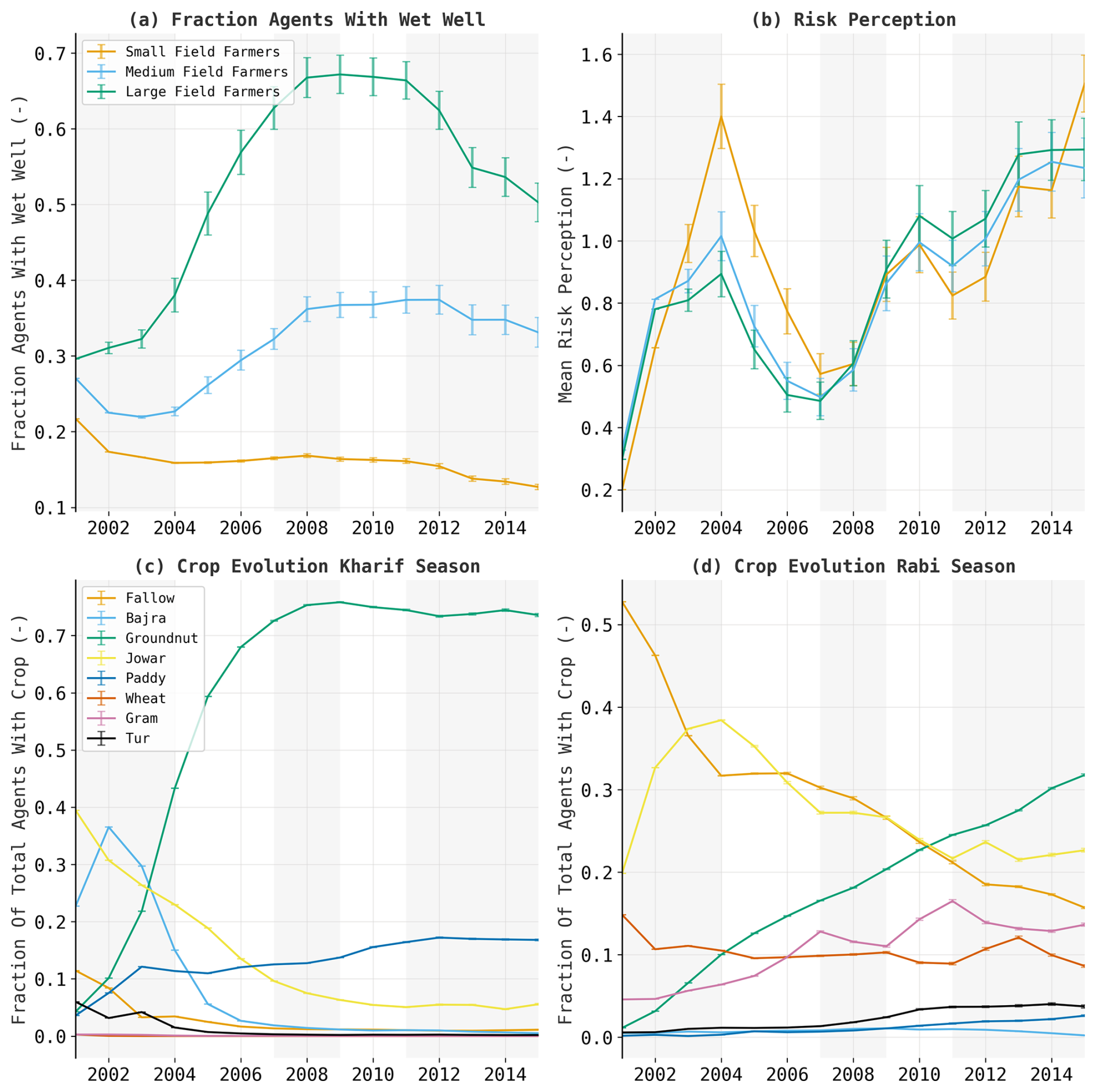
Figure 4 Evolution of wells, risk perception, and crops in the Bhima basin. (a, b) Farmers are categorized by field size into small (0th–33rd percentile, <0.82 ha), medium (33rd–67th percentile, 0.82–1.9 ha), and large (67th–100th percentile, >1.8 ha) groups: (a) the fraction of the total group with a wet well and (b) the mean risk perception of each group. (c, d) Evolution of the dominant crops in the (c) wet kharif and (d) dry rabi season. (a–d) Values are 60-run means, (a, b) error bars indicate the standard error, and light-grey areas indicate years where the average 1-month standardized precipitation evaporation index (SPEI) was below 0.

3 Results

3.1 Crop switching and well uptake in the adaptation scenario

Figure 4 shows how agent characteristics change over time for three different field sizes: large-scale (67th–100th percentile of size, >1.8 ha; green), medium-scale (33rd–67th percentile of size, 0.82–1.9 ha; blue), and small-scale (0th–33rd percentile of size, <0.82 ha; orange) farmers. Figure 4a shows the percentage of agents with wet wells. Uptake for large-scale farmer adaptation first slowly rises and subsequently speeds up after the first drought (2001–2004), alongside an increase in risk perception from the first drought. For medium-scale farmers, the fraction of wet wells initially decreases but then increases alongside a similarly heightened risk perception. For smallholder farmers, the number of well owners with groundwater access declines and only slightly recovers after the first drought, even though they have a higher risk perception compared to medium- and large-field farmers. This difference among well owners can be attributed to the varying interest rates available to them; smallholder farmers face the highest loan interest rates, while large-scale farmers benefit from the lowest rates (Appendix A1). Additionally, the initial investment costs per square meter are lower for farmers with more land and higher incomes. During the last drought (2011–2015), despite high risk perception, the proportion of farmers with wet wells accessing groundwater declines across all farm sizes (Fig. 4a and b). Wet-well use among large-scale farmers declines most in absolute terms, while smaller-scale farmers experience the largest percentage drop, with a reduction of more than half. The reduction in wells results from wells both exceeding their 30-year lifespan (Sect. S3.4.2) and drying up. However, the abrupt drop is likely due to wells drying up, as it occurs more quickly than the lifespan would suggest and aligns with a drop in groundwater levels (Fig. 6d).

In the wet kharif season, mainly groundnut increases in prevalence (Fig. 4c). Groundnut rose steeply in profitability compared to other crops during the study period (Appendix A2). Given that the decision theory primarily focuses on economic maximization, this could account for the sharp rise in groundnut cultivation, although such a steep rise is seemingly unrealistic. In the dry rabi season we see a large decrease in farmers who leave their field fallow (i.e., no crops), which is mainly replaced by cultivating groundnut, although there is a much greater heterogeneity of cultivated crops in the rabi season as compared to the wet kharif season (Fig. 4d). Furthermore, the increase and decrease in jowar cultivation, which is less water-intensive compared to groundnut and performs well during droughts (Singh et al., 2011), align very well with drought and non-drought periods.

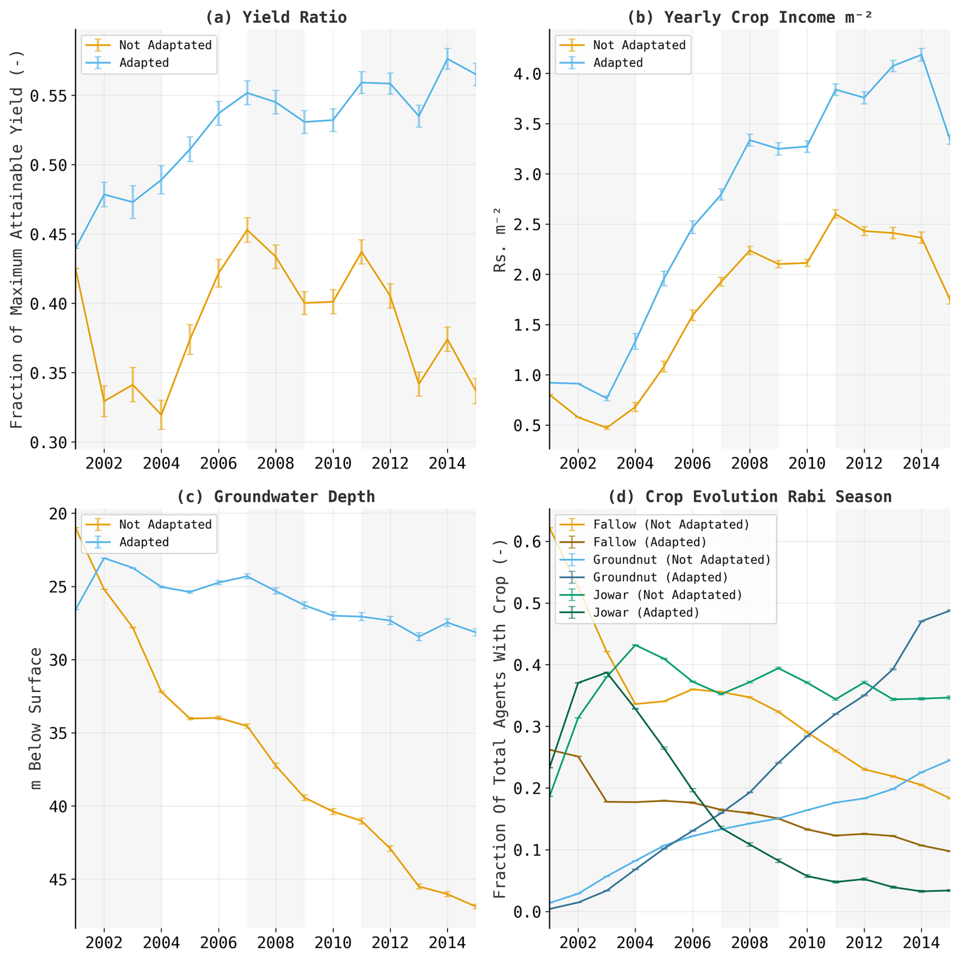
Figure 5 Evolution of the (a) yield ratio, (b) inflation-adjusted early income in rupees (INR) per square meter after harvesting and selling crops, (c) groundwater depth in meters below the surface, and (d) two main crops in the dry rabi season in the Bhima basin. Farmers are categorized by whether they have wells in each year into a not-adapted and adapted group. Light-grey areas indicate years where the average 1-month standardized precipitation evaporation index (SPEI) was below 0.

Figure 5a shows a large difference in the yield ratio between farmers with or without a well, likely stemming from the increased water reliability due to irrigation wells. Consequently, farmers with wells saw a yield ratio increase instead of a decrease during the first drought. Yearly crop income is approximately 30 % higher for farmers with wells (Fig. 5b), though incomes for both groups have increased due to switching to higher-priced crops. Importantly, these data show not only the effects of wells but also which farmers are able to initially afford wells, stemming from a prior higher yield, income, and lower groundwater levels. Groundwater levels are unexpectedly higher for farmers with wells (Fig. 5c), despite wells being the primary cause of groundwater depletion for most farmers (Figs. 6d and 7c). However, note that in the figure, farmers whose well dried up count as not adapted. Thus, when farmers with wells are in locations where groundwater recharge cannot keep up with extraction, their wells dry and they are switched to the not-adapted group. Subsequently, only farmers with wells where groundwater is not rapidly depleted or those who have recently installed wells remain in the adapted group, resulting in high average groundwater levels for this group. The extraction and hydroclimatic conditions at the farmers' locations where depletion matches the adapted group's average thus provide an estimate of the necessary circumstances to sustainably maintain wells. As long as these conditions are present, the increased yield ratios and income (Fig. 5a and b) can be maintained.

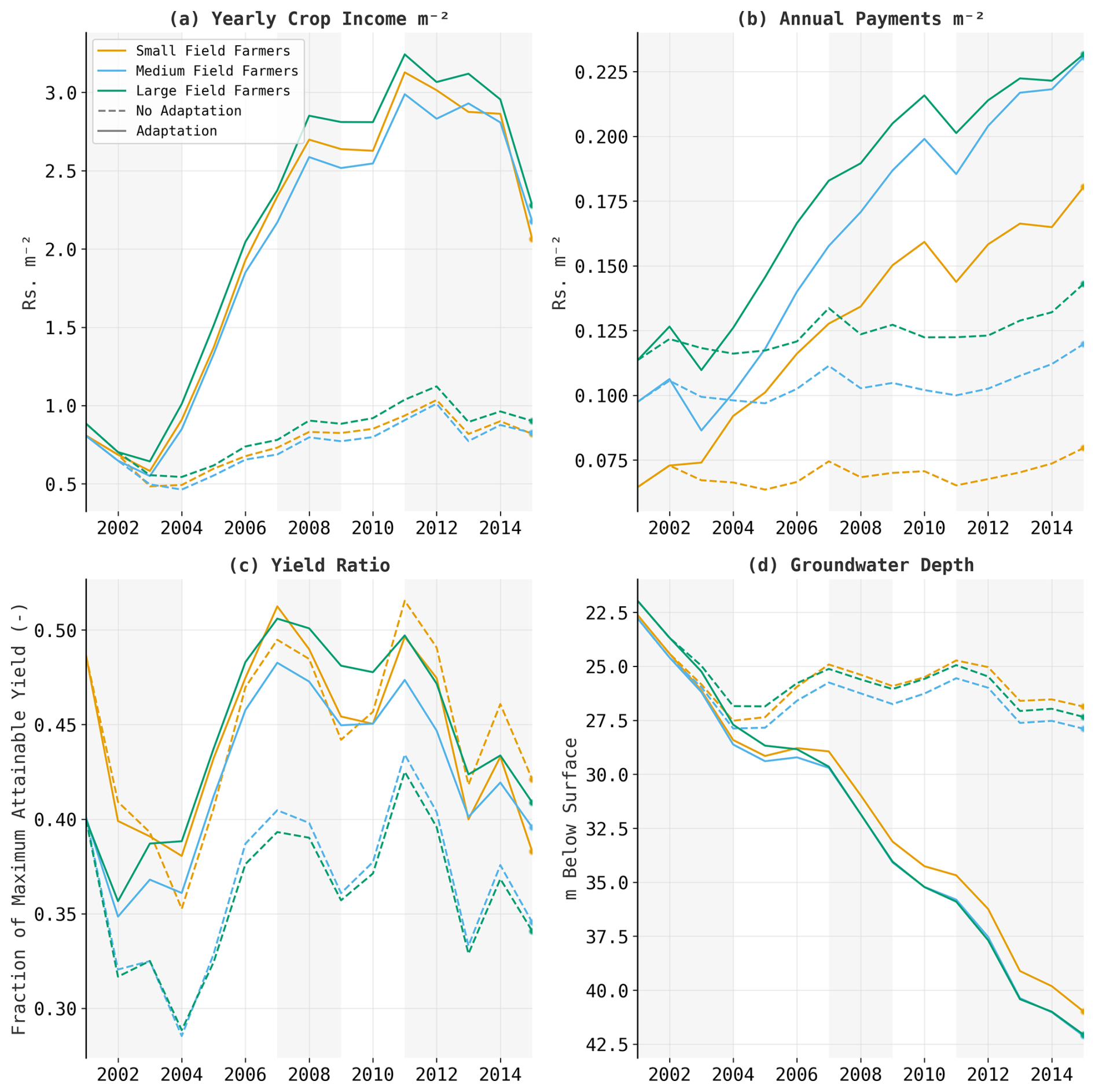
Figure 6 Evolution of income, loan payments, the groundwater depth, and the yield ratio in the Bhima basin for a scenario where agents adapt (filled line) and where they stick to their initial adaptations and crops (dotted lines). (a–d) Farmers are categorized by field size into groups of small (0th–33rd percentile, <0.82 ha), medium (33rd–67th percentile, 0.82–1.9 ha), and large (67th–100th percentile, >1.8 ha): (a) inflation-adjusted early income in rupees (INR, abbreviated in the figures as Rs.) per square meter after harvesting and selling crops; (b) inflation-adjusted yearly loan payments in INR per square meters, consisting of payments for cultivation costs, well loans, and microcredit in the case of crop failure; (c) average yield ratio of agent groups; and (d) groundwater depth in meters below the surface. Values are 60-run means, and light-grey areas indicate years where the average 1-month standardized precipitation evaporation index (SPEI) was below 0.

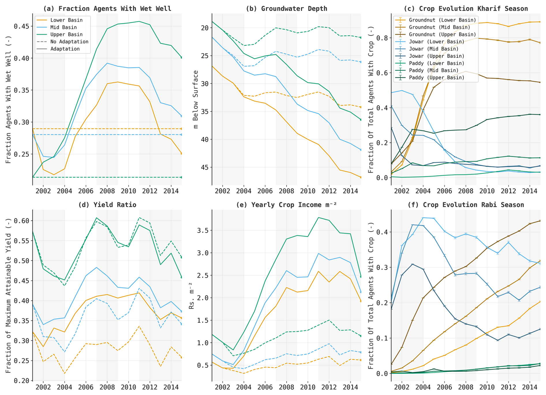
Figure 7 Evolution of wells, the groundwater depth, the two most cultivated crops in the dry rabi season, the yield, and the inflation-adjusted yearly crop income in rupees (INR) per square meter. Farmers are categorized by farmer elevation into lower-basin (0th–33rd percentile elevation), middle-basin (33rd–67th percentile), and upper-basin (67th–100th percentile) groups (a–f). Values are 60-run means, and light-grey areas indicate years where the average 1-month standardized precipitation evaporation index (SPEI) was below 0.

Figure 5d depicts the development of fallow, jowar, and groundnut cultivation during the dry rabi season. We show these crops as they are the most widely cultivated and dynamic (Fig. 4). In the kharif season, crop patterns are similar for both groups and follow the pattern of Fig. 4a. During the rabi season, agents both with and without wells switch to jowar during the first drought (2001–2004, Fig. 5d). However, after the initial drought, the percentage of agents with wells cultivating jowar is massively reduced, while the fraction without wells cultivating jowar remains stable. Furthermore, during the dry rabi season, more adapted agents cultivate groundnut, while fewer leave their land fallow. This contrast in cultivation patterns among well-irrigating and non-irrigating groups highlights the critical role of water availability in an agent's crop selection. If rainfall is ample, such as during the wet season, the patterns between farmers with and without wells are similar. However, in drier conditions, these patterns diverge because farmers with wells have greater water availability. This aligns with the patterns seen in Fig. 4.

3.2 Crop switching and well uptake in the adaptation vs. the no-adaptation scenarios

Figure 6 shows that during the first and most severe droughts from 2001 to 2004, the drop in the yield ratio of the no-adaptation scenario was 6 times worse (5 % vs. 30 % drop, Fig. 6c). These initial yield gains were likely due to a shift towards less water-intensive crops (jowar), as for medium-field farmers yields also increased, while their well uptake declined (Figs. 4a and 6c). Subsequent yield increases align better with well uptake, with larger-scale farmers achieving higher yields than smaller-scale ones. Furthermore, after the initial drought period, larger-scale farmers switched to higher-grossing but more water-intensive crops (Fig. 4d), as the yield ratios between small- and large-scale farmers were similar, while profits were higher. However, ultimately, well uptake dropped (Fig. 4a). Consequently, during the last drought from 2011 to 2015, the relative yield drop for larger-scale farmers was similar across both the adaptation and no-adaptation scenarios, contrasting with the decrease of 6 times seen during the first drought. Furthermore, the income fell 10 %–20 % more in the adaptation scenario (Fig. 6a).

In Fig. 6d, the groundwater levels in the no-adaptation scenario drop 5 m between 2001–2004 and then stabilize. Conversely, in the adaptation scenario, groundwater levels continue to decrease by an average of 1 m annually, stabilizing briefly during periods of positive SPEI (i.e., no droughts) and declining rapidly during droughts. The rate of groundwater decline is roughly the same for all farmers, regardless of farm size. The most recent rapid decline in 2011 corresponds with a decrease in wet wells (Fig. 4a), suggesting that this decline is primarily due to wells drying up. Since larger-scale farmers were the early adopters, their shallower wells were the first to dry up, which explains their more rapid decline compared to medium- and small-scale farmers (Fig. 4a). However, despite declining well uptake, loan payments remain high due to prior loans.

In Fig. 7, farmers are categorized as upstream (67th–100th percentile elevation), midstream (33rd–67th percentile), and downstream (0th–33rd percentile). Mid- to downstream farmers initially see a reduction in well use, with increases only occurring at the end of the first drought (2001–2004, Fig. 7a). This aligns with increased incomes late in the first drought as a result of the drought ending and switching to more profitable crops (Fig. A2). The crop switching has a dual effect: firstly, it boosts income, enabling agents to invest more in wells, and, secondly, it enhances well profitability, as now more water leads to a larger absolute increase in income. Upstream, the initial yield, income, and groundwater levels are higher. Higher groundwater levels reduce the price of wells, and higher incomes increase what agents can spend on wells. This reduces the effective investment costs, meaning the wells cost a smaller percentage of the agents' income, and more agents adapt. This causes upstream farmers to immediately adapt as the model starts, even during the first drought (2001–2004). Similar to the trends in Fig. 6d, groundwater levels quickly drop during droughts and stabilize when the SPEI is positive (Fig. 7b). This pattern is mirrored in well uptake, which increases until 2007 but halts in 2008, coinciding with a sharp decline in groundwater during the middle drought (2007–2009). During the last drought (2011–2015), groundwater levels rapidly fall again and well uptake substantially declines due to wells drying up. This decline intensifies downstream, resulting in downstream farmers having fewer wells than they initially had (Fig. 7a).

Despite fewer wells among downstream farmers, groundwater levels decline similarly to those in the middle and lower basins (Fig. 7b). Comparing this against spatially varying parameters between the lower, middle, and upper basins, we mainly see that upstream agent density is lower and precipitation is higher (Appendix A3). In the upper basin this means less additional irrigation water is required, resulting in more recharge and fewer agents abstracting groundwater per square kilometer. This also correlates with the shown higher yield and income (Fig. 7d and e).

During the wet kharif season, mid- and downstream farmers almost solely grow groundnut, whereas upstream paddy cultivation is also common (Fig. 7c). This follows the earlier shown pattern of higher water availability generally leading to more water-intensive crops. The yield ratio is highest upstream and lowest downstream, with the downstream area also showing a greater difference in yield between the adaptation and no-adaptation scenarios (Fig. 7d). This may be the effect of higher water demand upstream, which is caused by more water-intensive crops offsetting more of the supply gains. This is also reflected in a lower yield ratio compared to the no-adaptation scenario, even though there are more agents with wells.

For mid- and downstream farmers, yield ratios increased during the first drought compared to the no-adaptation scenario, even though well uptake declined (Fig. 7a and d). Similar to what was discussed regarding Figs. 4–6, this increase was due to a shift toward a less water-intensive crop (jowar, Fig. 7f). Subsequently, as water availability increased, the prevalence of jowar declined, while groundnut, which requires more water than jowar but less than paddy, continued to rise due to its steep price increase (Fig. 7f, Appendix A2). This pattern again followed water availability, as this was more pronounced for the mid- and upstream farmers. The economic maximization through crop switching boosted incomes without requiring additional water from wells (Fig. 7a and e). However, yields in the adaptation scenario for mid- and downstream farmers continued to rise compared to the no-adaptation scenario. Furthermore, both yields fell less during the middle drought. This pattern aligns with the initial rise in well usage for these groups (Fig. 7a). Ultimately, well uptake fell, and during the last droughts (2011–2015) yield ratios fell by 18 %–22 %, approximately equal to the amount in the no-adaptation scenario. However, from 2011 to 2015, crop income in the adaptation scenario fell by 25 %–35 %, a 10 %–15 % greater decline compared to the no-adaptation scenario. This is a larger fall than what only the yield ratios would suggest and can be explained by a simultaneous drop in prices for the main cultivated crops (Appendix A3).

4 Discussion and recommendations

In this study, we further developed a large-scale socio-hydrological ABM to assess the adaptive responses of different farmer agents under consecutive droughts. We show that farmers with more financial resources invest in irrigation quickly when a drought occurs, whereas farmers with fewer resources or no wells switch to less water-intensive crops to increase yields (Birkenholtz, 2009, 2015; Fishman et al., 2017). After the first drought, as risk perception is still high and income has increased, well uptake also increased among farmers with fewer financial resources. In the short term, this increased the area's income and resilience, reflected in rising yields and income over consecutive droughts. However, similar to reservoir supply–demand cycles (Di Baldassarre et al., 2018), the widespread adoption of wells led to an increase in water-intensive crops and growth of crops during the dry season, which in turn raised water demand. During wet periods the available groundwater could support this demand, but during dry periods the groundwater rapidly declined. Consequently, despite being less severe than the first, the last drought resulted in many wells drying up quickly and yields declining. Furthermore, homogeneous cultivation as a result of economic maximization made the region more sensitive to market price shocks. This was seen from 2013 to 2015, where crop market prices of the main cultivated crops dropped, which led to a much larger drop in farmers' average income compared to the no-adaptation scenario. Thus, although drought vulnerability initially decreased and incomes rose, ultimately, a farmer's adaptive responses under consecutive droughts increased drought vulnerability and impact. This underscores the importance of considering consecutive events, as focusing solely on the first event would overlook the ultimate impact. Suggested policies to address groundwater decline and well drying while maintaining higher incomes include promoting efficient irrigation technologies (Narayanamoorthy, 2004), implementing fixed water use ceilings (Suhag, 2016), encouraging rainwater harvesting (Glendenning et al., 2012), or combinations of these all techniques (Wens et al., 2022).

The maladaptive path of tube well irrigation expansion, growth of water-intensive crops, and subsequent rapid depletion of groundwater and resulting economic decline we simulated here have been commonly observed in India (Birkenholtz, 2014; Pahuja et al., 2010; Roy and Shah, 2002; Solomon and Rao, 2018). Previous studies modeling the economics of wells show the income and groundwater fluctuations from wells and crop changes occurring gradually (Robert et al., 2018; Sayre and Taraz, 2019). Aside from investment costs, they show profits and groundwater levels rising and falling gradually over time, with the simulations never experiencing shocks. However, we observe that this process is not steady but is instead characterized by periods of stabilization during wet periods and rapid declines in groundwater levels and incomes during dry periods. Additionally, under consecutive droughts, we see social (i.e., continued loan payments, crop price drops) (Solomon and Rao, 2018) and ecological shocks (i.e., lower groundwater levels, drought) coinciding (Folke et al., 2010). Therefore, agricultural decline may occur more suddenly and rapidly in an approach using socio-hydrological systems than what previous studies predict (Manning and Suter, 2016; Robert et al., 2018; Sayre and Taraz, 2019). Such sudden shocks are harder to adapt to, potentially leading to more severe impacts or disasters (Rockström, 2003). Thus, for future analyses, we recommend transitioning to similar coupled agent-based hydrological models, combined with climate data, to identify areas where drought risk is or will be high.

We also observed that adaptive patterns are spatiotemporally heterogeneous. For example, the farmers' location determined the number of wells that could be held before depleting groundwater levels, influenced by factors like precipitation and agent density. Water availability, resulting from precipitation and irrigation, along with market dynamics, influenced crop choices. This led to varied cropping patterns as prices fluctuated between wet and dry periods, seasons, and locations upstream or downstream. Furthermore, at an individual scale, we observed that variations in farm size, access to credit, time preferences, or risk attitudes influenced farmers' adaptation decisions. Building on our demonstration of the impact of varying hydroclimatic conditions and farmer characteristics on adaptation behavior, as well as the substantial effects of this behavior on a river basin's hydrology, we again highlight the value of large-scale coupled socio-hydrological models. These models can further enhance understanding of both basin hydrology and farmer behavior. This is needed to design policies such that they, for example, minimize overall impacts and specifically reduce impacts on smallholder farmers (Wens et al., 2022). By further exploiting our methods, it is possible to attempt to identify policies that can slow the expansion of wells in areas where it is unsustainable, while simultaneously avoiding interference in regions where growth is more sustainable, which is recommended as sustainable well use can also greatly improve water resilience (Blakeslee et al., 2020; Pahuja et al., 2010; Roy and Shah, 2002; Shah, 2009; Solomon and Rao, 2018). Furthermore, these novel approaches can help to determine which adaptation alternatives and policies can decrease drought vulnerability while simultaneously being financially attractive enough to see adaptation beyond the village scale (Fishman et al., 2017).

In this study we were able to model emergent patterns as a result of many combined small-scale processes due to human behavior under consecutive droughts at a river basin scale and quantitatively assess their hydrological and agricultural impacts. The model almost exactly replicated the commonly observed stages of well expansion; initial higher resilience; groundwater overextraction due to a shift to high-value water-intensive crops; groundwater table decline; and subsequent well failure, indebtedness, and agricultural decline in India, as detailed by Birkenholtz (2014), Pahuja et al. (2010), Roy and Shah (2002), and Solomon and Rao (2018). Secondly, it provides a much better representation of the accelerated groundwater decline during droughts observed in the field (Birkenholtz, 2014; Pahuja et al., 2010; Udmale et al., 2014), which was not captured in previous well-modeling studies (Robert et al., 2018; Sayre and Taraz, 2019). Thirdly, our results reflect a similar observed pattern of crop choice, where farmers facing water scarcity during and after droughts switch to drought-tolerant crops (Birkenholtz, 2009; Udmale et al., 2014). Lastly, the water table decline of approximately 1 m yr⁻¹ fits the many reports of groundwater decline of 1002 m yr⁻¹ by Singh and Singh (2002). However, although we anticipated that changes in risk perception would have a stronger impact on well uptake, our results and the sensitivity analysis (Fig. B1) show that economic considerations were predominantly the driving factor. This aligns with other studies which mention drought response as a major driver of well uptake (Pahuja et al., 2010; Shah, 2009) but call social and economic aspirations the main driver (Solomon and Rao, 2018). Additionally, the 2011–2012 Agriculture Census reported that only approximately 25 % of farmers in our area owned a well (Agricultural Census India, 2023b), which is lower than what our findings suggest. This discrepancy likely stems from the timing of our simulations not aligning with the study area's current stage of the cycle of well expansion and decline (Fig. 20 of Roy and Shah, 2002). In reality, well expansion occurred before the first census and simulation period (Central Ground Water Board, 1995) and declined from 2001 to 2011–2012 (Agricultural Census India, 2023a, b). Consequently, the area's groundwater levels should have been lowered and the cost of adaptation should have increased. However, as there were no spatial (longitudinal) groundwater level observations available to initialize or calibrate the model with, our simulation had to move through the first stages of well expansion (Roy and Shah, 2002) before groundwater levels and adaptation costs matched those of the area's. Thus, our well uptake is lagging behind. For these reasons and given that other inputs like drought loss thresholds are theoretical (Bubeck et al., 2012; Kahneman and Tversky, 2013; Ribeiro Neto et al., 2023) and not specifically defined for droughts, this paper focuses on patterns, variations among farmers, locations, and scenario differences rather than on temporally specific absolute values. For future studies where timing is more important, e.g., those focused on future policy scenarios, initializing groundwater levels, by either lowering them during calibration or collecting observations, is crucial. In general, we highly recommend the development of detailed spatial and behavioral data to improve the accuracy of large-scale ABMs. Regarding agents' crop choices, we observed a trend toward highly homogeneous cultivation of certain crops that experienced significant price increases. Although a progression towards uniform cultivation of crops has been observed under similar circumstances (Birkinshaw, 2022) and groundnut is described as being by far the most cultivated crop (Batchelor et al., 2003; Birkenholtz, 2009), the degree seen here is unlikely. We incorporate rational economic decisions influenced by subjective risk perception as a result of experiencing droughts into our analysis, as this was the central focus of our study. However, other subjective behaviors exist, such as decisions influenced not by personal benefit assessments but by perceptions of others' beliefs, cultural norms, attitudes, or habits (Baddeley, 2010). Including this type of behavior in future research may reduce homogeneity; however, no behavioral theory perfectly encompasses all adaptive behaviors (Schrieks et al., 2021). Therefore, we recommend keeping the SEUT while incorporating a market feedback that lowers the profitability of commonly cultivated crops due to increased cultivation costs and reduced market prices, calibrated with observed prices. Alternatively, we suggest adding a calibrated unobserved cost factor for all crops (Yoon et al., 2024). Both modulate the profitability of crops and reduce the modeled divergence from historical patterns. Furthermore, subsistence farming, which involves cultivating crops for household consumption, could reduce homogeneity as well (Bisht et al., 2014; Hailegiorgis et al., 2018). Subsistence farms cultivate more diverse crops and take up most of a smallholder farmer's cultivated area (Bisht et al., 2014). A proposed model implementation could mandate that all farmers dedicate one plot to subsistence crops. This would limit the smallest-scale farmers to their initial crop rotations, while larger-scale farmers would be free to cultivate commercial crops on their remaining land. Incorporating perceptions of economic conditions could also make crop choice modeling more realistic by farmers forecasting and adjusting future crop prices based on their likelihood. For instance, while current high prices for groundnuts might not persist, government-regulated sugarcane prices provide certainty. Thus, e.g., risk-averse farmers might favor the predictability of sugarcane over crops with more volatile pricing. Lastly, while GEB efficiently simulates agents at a one-to-one scale, exploring how aggregate phenomena shift with varying degrees of agent aggregation could be valuable, since higher levels of aggregation might optimize model runtimes.

5 Conclusions

In this study, we assess the adaptive responses of heterogenous farmers under consecutive droughts at the river basin scale in the Bhima basin, India. To do so, we further developed a large-scale socio-hydrological agent-based model (ABM) by implementing the subjective expected utility theory (SEUT) alongside heterogeneous farmer characteristics and dynamic adaptation costs, risk experience, and perceptions to realistically simulate many individuals' behavior. From the emergent patterns of all individuals' behavior under consecutive droughts we were able to assess river basin scale patterns and come to these three main conclusions.

First, a farmer's adaptive responses under consecutive droughts ultimately led to higher drought vulnerability and impact. Although a farmer's switching of crops and uptake of wells initially reduced drought vulnerability and increased incomes, subsequent crop switching to water-intensive crops and intensified cropping patterns increased water demand. Furthermore, the homogeneous cultivation encouraged by economic maximization made the region more sensitive to market price shocks. These findings highlight the importance of looking at consecutive events, as focusing solely on adaptation during first events would overlook the ultimate impact.

Second, the impacts of droughts on (groundwater-irrigating) farmers are higher and can happen more suddenly in a socio-hydrological system under realistic climate forcings compared to what just gradual numerical economical models can predict. This is because groundwater depletion happens in periods of stabilization and rapid reduction instead of gradually and because ecological shocks (i.e., droughts) and social shocks (i.e., crop price drops) can coincide to rapidly decrease farmer incomes.

Third, adaptive patterns, vulnerability, and impacts are spatially and temporally heterogeneous. Factors such as market prices, received precipitation, farmers' characteristics and neighbors, and access to irrigation influence crop choices and adaptation strategies. This variability underscores the benefits of using large-scale ABMs to analyze specific outcomes for different groups at different times.

This research presents the first analysis of a farmer's adaptive responses under consecutive droughts using a large-scale coupled agent-based hydrological model with realistic behavior. We emphasize the added value of employing coupled socio-hydrological models for risk analysis or policy testing. We recommend using these models to, for example, test policies designed to minimize overall impacts or to minimize them for smallholder farmers. Further research could also explore alternative adaptations to wells that reduce drought vulnerability and are financially viable enough to encourage wider adoption. Lastly, we advocate for research aimed at developing detailed regional data to improve the accuracy of large-scale ABMs, along with acquiring empirical data on behavioral aspects to refine behavioral estimates.

Appendix A: Additional figures

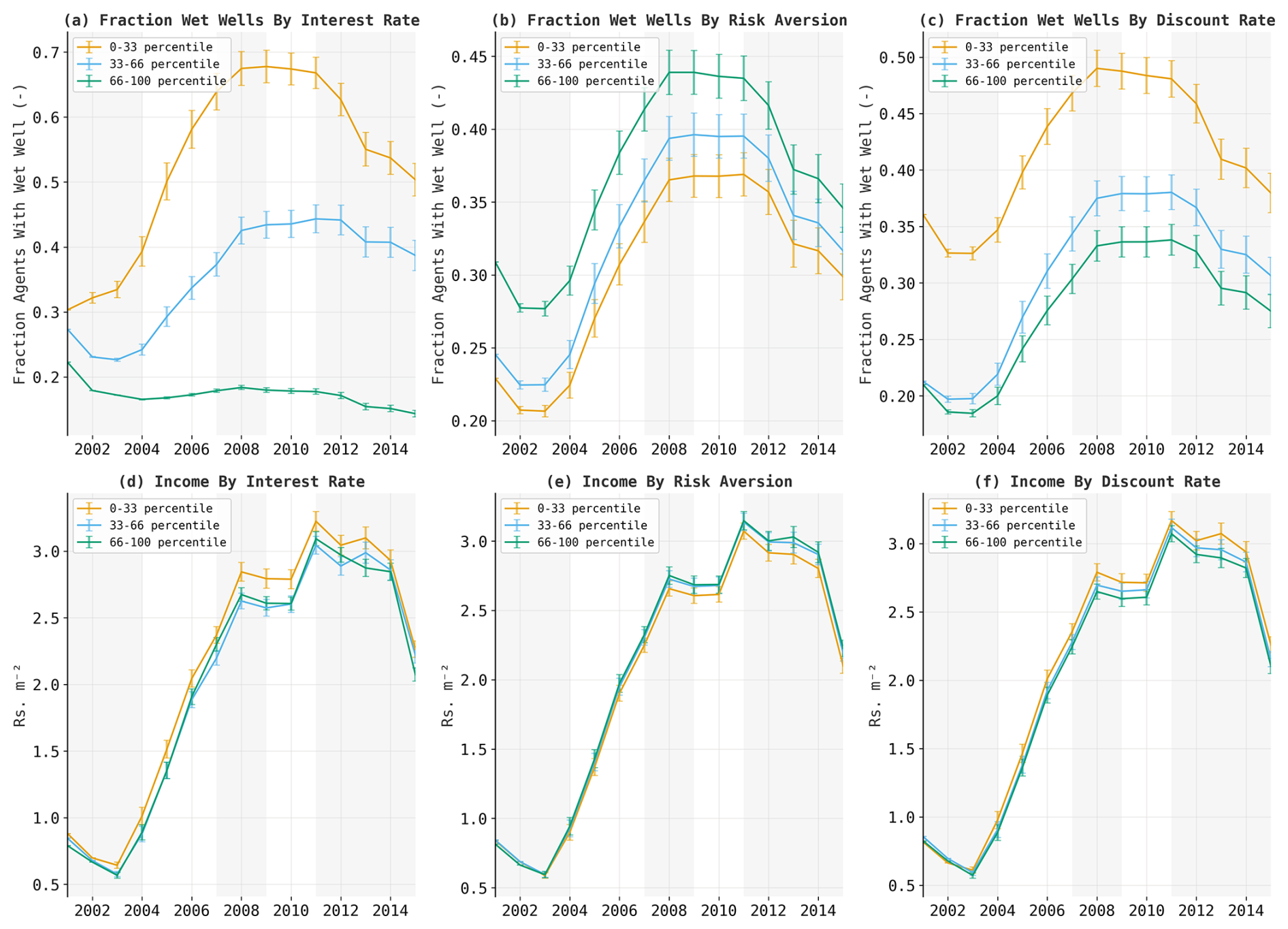
Figure A1 Well uptake and income grouped based on the agent's interest rate, risk aversion, and discount rate. The values indicate the means of 60 runs, while the error bars indicate the standard error.

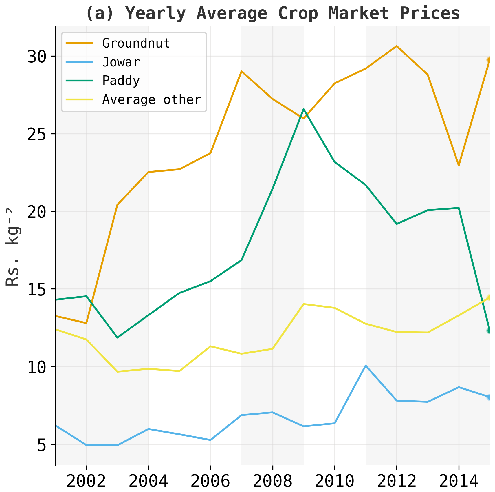
Figure A2 Inflation-adjusted crop market prices for groundnut, jowar, paddy, and the mean of all other crops.

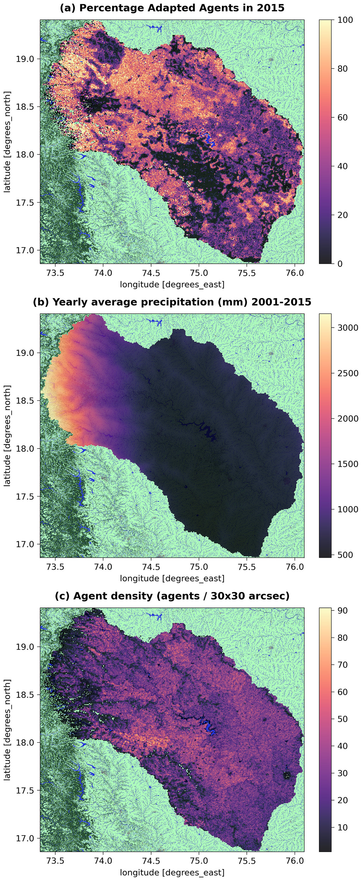
Figure A3 Spatial patterns of (a) adaptation, (b) precipitation, and (c) agent density in the Bhima basin.

Appendix B: Model sensitivity analysis

B1 Sensitivity analysis method description

Sensitivity parameters were changed differently per parameter. The function latin.sample using Latin hypercube sampling from SALib (Iwanaga et al., 2022) was used to generate 300 sets of values of each sensitivity parameter between their min and max. The min and max were used as inputs either to change the absolute values of a parameter (drought loss threshold), to change the distributions of all agents' values (risk aversion, discount rate), or to change all agents' individual parameters with a fixed rate (interest rate).

B1.1 Risk aversion

See Sect. 2.5 on how the initial risk aversion was determined. To change this, this distribution was normalized and rescaled using a new standard deviation, which was a latin.sample value between the given min and max.

B1.2 Discount rate

Similar to risk aversion, now instead of the standard deviation, the mean was sampled between the min and max and used to rescale the distribution.

B1.3 Interest rate

Each agent's individual interest rate (Sects. 2.5 and S2.1.4) was multiplied with a sampled value between the given min and max.

B1.4 Well cost

The well cost factor is determined by adjusting the fixed and yearly costs by an absolute factor. This absolute factor adjusts the price based on a normal distribution of values. The standard deviation is 0.5 (50 % higher/lower price), and the mean is 1 (no price change). The latin.sample function then samples quantile values between 0 and 1 and uses the standard deviation and mean to calculate the adjustment factor. Thus, the percent adjustment factor follows a normal distribution around the original price (Eq. 1).

Table B1 Min and max settings of the sensitivity analysis.

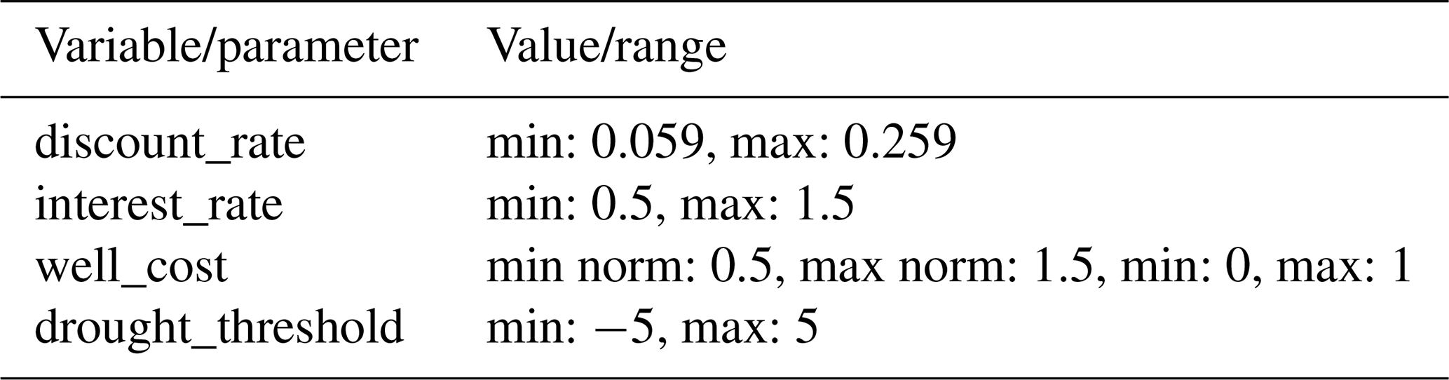
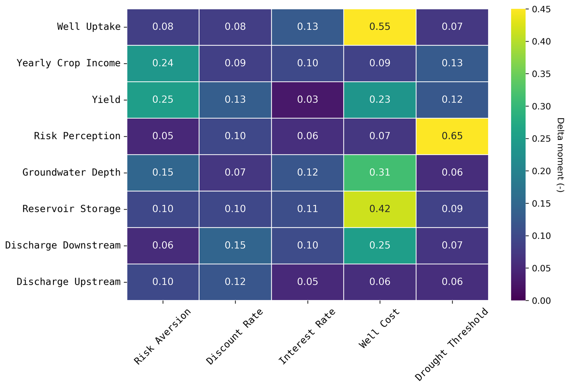
Figure B1 Delta moment sensitivity analysis. Values indicate how sensitive an output factor (y axis) is to the influence of a specific input factor (x axis), in relation to the influence of all other input factors. The output consists of the number of wells, the yearly crop income, the yield, risk perception, the groundwater depth, reservoir storage, and discharge up- and downstream. The changed input parameters consist of risk aversion, the discount rate, the interest rate, well cost, and the drought threshold.

B1.5 Drought loss threshold

An absolute value was added to or subtracted from the drought loss threshold based on the sampled values between the min and max.

B2 Sensitivity analysis results

Our results show that well uptake is highly sensitive to well cost and not very sensitive to the drought threshold. Diving deeper into this relation, Fig. 8 shows that although well cost substantially affects the adoption of wells and yield, its impact on income is minimal compared to other factors. This notion is supported by Figs. 4 to 7, which reveal that many farmers cannot afford wells regardless of cost changes and that decreasing groundwater levels result in the loss of wells. Thus, although the effect of wells is large for farmers with wells (Fig. 4), a large group remains without wells throughout the basin. In contrast, risk aversion substantially affects both well adoption and crop selection, and crop selection is relevant to all farmers. Furthermore, crop selection is especially impactful as the price of groundnut, the primary crop farmers switch to in the main season, doubled relative to other crops (Fig. 7g). This illustrates that a farmer's adaptive behavior is a mix of climate and market dynamics.

However, Fig. 8 shows that well cost substantially influences all hydrological parameters except upstream discharge. Recorded in regions with higher precipitation and fewer agents (Appendix A3), upstream discharge shows little sensitivity to well cost, suggesting groundwater extraction makes up a smaller fraction of total river inflow. Similar to income, yield reacts to risk aversion through crop choice. Risk perception is sensitive to the drought loss threshold and is the second most influential factor for income.

Appendix A1 shows that the interest rate significantly impacts farmers' ability to afford wells and influences their income more than risk aversion and the discount rate. This contrasts with Fig. 8, which shows that all three input factors equally affect well uptake and that risk aversion and the discount rate are more important for income. This likely stems from the sensitivity analysis parameters, where the change in the interest rate is based on a factor multiplied by the agent's initial rate, leading to minimal variation if the initial value is low. Furthermore, agents with higher initial interest rates are already not adapting (Appendix A1) and thus are only sensitive to (one-way) decreasing interest changes.