the Creative Commons Attribution 4.0 License.
the Creative Commons Attribution 4.0 License.
 | 15 Feb 2024
Evaluating pySTEPS optical flow algorithms for convection nowcasting over the Maritime Continent using satellite data
Joseph Smith
Cathryn Birch
John Marsham
Simon Peatman
Massimo Bollasina
George Pankiewicz
The Maritime Continent (MC) regularly experiences powerful convective storms that produce intense rainfall, flooding and landslides, which numerical weather prediction models struggle to forecast. Nowcasting uses observations to make more accurate predictions of convective activity over short timescales (∼ 0–6 h). Optical flow algorithms are effective nowcasting methods as they are able to accurately track clouds across observed image series and predict forward trajectories. Optical flow is generally applied to weather radar observations; however, the radar coverage network over the MC is not complete and the signal cannot penetrate the high mountainous regions. In this research, we apply optical flow algorithms from the pySTEPS nowcasting library to satellite imagery to generate both deterministic and probabilistic nowcasts over the MC. The deterministic algorithm shows skill up to 4 h on spatial scales of 10 km and coarser and outperforms a persistence nowcast for all lead times. Lowest skill is observed over the mountainous regions during the early afternoon, and highest skill is seen during the night over the sea. A key feature of the probabilistic algorithm is its attempt to reduce uncertainty in the lifetime of small-scale convection. Composite analysis of 3 h lead time nowcasts, initialised in the morning and afternoon, produces reliable ensembles but with an under-dispersive distribution and produces area under the curve scores (i.e. ratio of hit rate to false alarm rate across all probability thresholds) of 0.80 and 0.71 over the sea and land, respectively. When directly comparing the two approaches, the probabilistic nowcast shows greater skill at ≤ 60 km spatial scales, whereas the deterministic nowcast shows greater skill at larger spatial scales ∼ 200 km. Overall, the results show promise for the use of pySTEPS and satellite retrievals as an operational nowcasting tool over the MC.
- Article
(3810 KB) - Full-text XML
- BibTeX
- EndNote


The “Early Warnings For All Initiative” was launched by the United Nations in November 2022 and calls for the whole world to be covered by early warning systems by the end of 2027 (World Meteorological Organization, 2023). It focuses on poorer countries in Asia, Africa, South and Central America, and the Pacific and motivates the development of early warning weather systems for these regions.
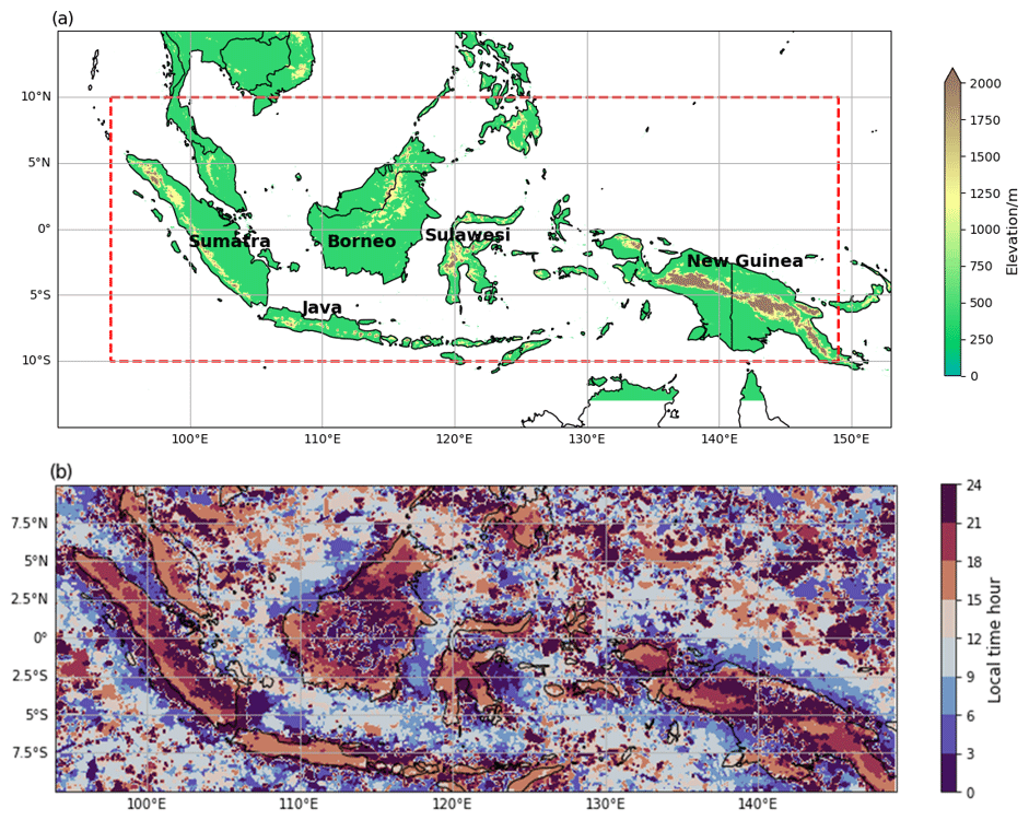
Figure 1(a) Orographic map of the Maritime Continent showing the domain over which the nowcasts were generated and the domain over which they were evaluated (dotted red line). (b) The diurnal cycle of peak rainfall within the evaluation region (interpolated to local solar time) using the Global Precipitation Measurement dataset (Hou et al., 2014) from December, January and February 2001–2020.
The Maritime Continent (MC) is a region of Southeast Asia that includes the countries of Indonesia, Malaysia, the Philippines, Papua New Guinea, Brunei and Timor-Leste. It is a complex mix of land and ocean with major islands such as Sumatra, Java, Borneo and New Guinea, making it the largest archipelago on Earth (Fig. 1a). It is also one of the wettest places on Earth with its complex topography and location across the Equator, making it a hotspot for extreme weather. The region often experiences natural disasters such as flooding and landslides that have disastrous effects on already very poor areas. Easterly trade winds blow warm water across the Pacific into the MC, creating a “warm pool” around the region (Dayem et al., 2007), which, when combined with its proximity to the Equator and the inter-tropical convergence zone, provides favourable conditions for deep convection. The large amounts of latent heat released from this convection mean that the region is often referred to as the “boiler box” of the tropics as it plays a crucial role in contributing to the global atmospheric circulations (the Hadley and Walker cells), in turn affecting both local and global weather systems (Ramage, 1968).
The MC's strong diurnal cycle (shown in Fig. 1b by the spatial variation in timings of peak rainfall) is one of its dominant drivers of convective activity (Yamanaka, 2016). It has typical characteristics of most diurnal cycles across the tropics (Yang and Slingo, 2001), starting with peak solar insolation around midday. This starts to form a land–sea temperature contrast due to the lower heat capacity of the land. A sea breeze then develops blowing on land, often triggering convection which builds into the late afternoon and evening. Many islands in the MC also contain mountains close to the coast with altitudes of over 2000 m (e.g. Sumatra). Orographic lifting driven by the mountains can further enhance the convection (Mori et al., 2004). Into the late evening and overnight this convection propagates offshore until the early morning the following day, leaving clear skies over land in the morning for strong solar insolation to restart the process.
Numerical weather prediction (NWP) models struggle to represent the moist convection that dominates weather in the MC, with coarser-resolution models often initiating convection too early in the day (Porson et al., 2019) or under-estimating the amount of rainfall (Qian, 2008). Ferrett et al. (2021) show that the ensemble forecasts from a higher-resolution, convective-scale configuration of the Met Office Unified Model, with 4.5 km horizontal grid spacing over Indonesia, only start to show skill (during the first day after initialisation) when coarsened up to spatial scales of ∼ 150 km. Mesoscale convective systems are defined as having spatial scales of at least ∼ 100 km, and so convective-scale models cannot be relied upon to skilfully resolve impactful storms over the MC.
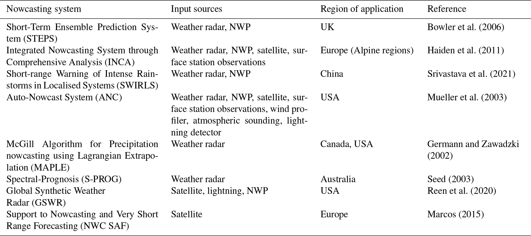
Table 1Information on some of the state-of-the-art nowcasting systems that are currently in operational use around the world.
Nowcasting is the process of obtaining current observations of the atmosphere and using them to generate rapid, short-term (typically ∼ 0–6 h ahead) predictions of the future atmospheric state (Roberts et al., 2022). It requires real-time observations (e.g. from weather radar) as an input and the application of predictive techniques to forward-propagate these observations. Unlike NWP models, nowcasting tools do not use large sets of complex numerical equations in order to model the atmosphere. Instead, they use cutting edge computational techniques such as optical flow and artificial intelligence algorithms, enabling them to generate useful output at near-instantaneous timescales (Ayzel et al., 2020; Han et al., 2019; Gijben and de Coning, 2017).
Currently, there are a number of state-of-the-art nowcasting systems in operation around the world, typically based in developed countries, which take advantage of large weather radar networks to provide near-instant, wide spread data coverage of precipitation. There are, of course, many operational systems in use globally, but Table 1 covers some of the most advanced ones.
Weather radar networks are expensive to implement, maintain and often not suitable for regions with mountainous terrain (e.g. the MC), meaning the types of nowcasting systems listed in Table 1 cannot always be implemented. There is, therefore, a widespread interest within nowcasting research in the use of satellite data as the main source of input, especially in the tropics, which can provide constant, widespread coverage of the Earth's atmosphere from space. The advancement of satellite technology in recent years has given us access to data on increasingly higher spatial and temporal resolutions (e.g. Line et al. (2016) use 1 min retrievals of 1 km resolution imagery for forecasting), allowing finer detail of cloud structures to be observed and more accurate tracking of weather systems (Sieglaff et al., 2013). This provides the basis for extrapolation nowcasting methods that use the tracked history of weather features (e.g. storms) to calculate motion vectors, which the features are then propagated along to create future predictions (Burton et al., 2022; Vila et al., 2008; Line et al., 2016). The vast volume of satellite data also makes nowcasting a suitable candidate for the application of machine learning methods to make future predictions of the atmosphere. Most commonly, studies have trained machine learning models to take in consecutive satellite images as input and then output (nowcast) the future consecutive images (Lebedev et al., 2019; Lagerquist et al., 2021).
The MC itself has received little attention in the field of nowcasting, despite the region experiencing regular intense convective activity affecting the lives of millions. The Indonesian network consists of 42 weather radars (Permana et al., 2019) but is sparse relative to the size of the country; the country is highly mountainous and experiences communication issues between sites, meaning real-time full radar coverage of the region is not possible (Permana et al., 2019). One of the radars within the network was used by Ali et al. (2021) to nowcast two rainfall events over southern Borneo. On the other hand, satellite data were used by Harjupa et al. (2022) to apply the Rapidly Developing Cumulus Area algorithm (Sobajima, 2012) to a region of western Java to predict heavy rainfall for 77 events. The limited sample size and domain of these studies makes it difficult to understand how effective the methods are for other regions of the MC. There is, therefore, a need to test nowcasting tools that can be applied and evaluated across the entire MC domain.
pySTEPS (Pulkkinen et al., 2019) is a free, open-source Python library that provides modules for a variety of optical flow-based nowcasting methods (see Sect. 2.1a for optical flow description). The library is designed for use on radar data and has been used to show skilful prediction of stratiform precipitation in the mid-latitudes (Han et al., 2022; Imhoff et al., 2020). To the best of the authors' knowledge, the only study that has applied pySTEPS to satellite data over the tropics is Burton et al. (2022), who produced nowcast skill up to a 4 h lead time over West Africa. It is this result that motivates the application of pySTEPS to the MC.
This paper presents the evaluation of both deterministic and probabilistic nowcasts produced by applying pySTEPS to satellite data over the MC. The aim is to highlight their strengths and weaknesses and demonstrate their potential use as an operational nowcasting system.
2.1 Data
This study uses brightness temperature (BT; the temperature a black body would need in order to emit the radiance detected by a satellite) data from the Himawari-8/Himawari-9 satellites as input to the nowcasting algorithms. Himawari-8 and Himawari-9 are passive geostationary satellites with 16 band channels ranging from 0.47 to 13.3 µm, covering parts of the visible, near-infrared and infrared (IR) spectrum (Bessho et al., 2016). Hourly BT data from channel 13 on board Himawari-8/Himawari-9 have been used, which detect IR radiation with a wavelength of 10.4 µm. The full-disc images are transformed to a Cartesian grid with a grid spacing of 2 km, using the gdalwarp command from the Geospatial Data Abstraction Library (Rouault et al., 2023). Convective clouds can be clearly identified in BT maps as they have cold tops relative to the surface of the Earth. The data are selected from the December, January and February (DJF) season, which is the peak season for convection over the MC (Birch et al., 2016), for five seasons from 2015/2016–2019/2020 (data retrievals of Himawari-8 began in 2015; Bessho et al., 2016).
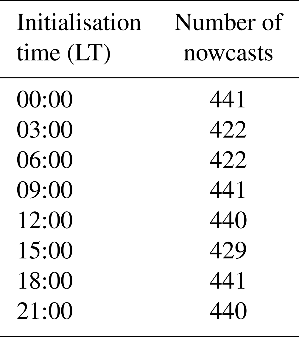
In this study, nowcasts were produced using three BT maps as input, spaced evenly apart by 1 h, starting with the latest observation. A total of 3476 nowcasts were produced for initialisation times every 3 h from 00:00 LT to 21:00 LT to incorporate the diurnal variability of weather over the MC, with the number of nowcasts at each initialisation time shown in Table 2. In order to avoid issues of new convection entering the edge of the domain, which cannot be reproduced (optical flow can only propagate convection that exists in the domain at the nowcast initialisation time), the nowcasts were first produced using BT data on a 15∘ S–15∘ N, 90∘–153∘ E domain and then evaluated on a 10∘ S–10∘ N, 94–149∘ E domain, which still includes the major islands of the MC (Fig. 1a).
Table 2The number of nowcasts that were produced at each initialisation time throughout the day.
2.2 Methods
2.2.1 pySTEPS/optical flow
pySTEPS provides a well-documented framework that allows users to employ optical flow algorithms for both deterministic and probabilistic nowcasting approaches, as well as a range of verification techniques. Optical flow is a computer vision technique that generates velocity fields to describe the apparent motion of objects across consecutive images (Horn and Schunck, 1981). The key assumption of optical flow is that each pixel intensity remains constant across all images as it is advected. Given is the intensity of a pixel at time t=0, this results in
where Δt is the time between image frames. Applying a Taylor series expansion to Eq. (1) leads to
where and are the velocity components of the motion field. Equation (2) is known as the optical flow equation. , and can be calculated as they represent the image gradients over space and time, whereas U and V are unknown meaning. Equation (2) represents an underdetermined system that cannot be solved directly. Optical flow methods attempt to get round this by applying various spatial constraints to U and V. Section 2.2.2 and 2.2.3 will describe the two optical flow methods within pySTEPS that were used in this study.
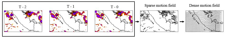
Figure 2An example (using BT over Sumatra) of how a motion field is generated using the LK method. Features are identified and tracked across the three input images (T−0, T−1 and T−2) to generate the sparse motion field. The sparse motion field is then interpolated onto the rest of the domain to produce the dense motion field.
2.2.2 Lucas–Kanade deterministic algorithm
The Lucas–Kanade algorithm (LK; Lucas and Kanade, 1981) is an optical flow method that assumes, for a given pixel, the eight immediately surrounding pixels move along with that given pixel. This assumption results in nine separate versions of Eq. (2) (eight from the surrounding pixels and one from the given pixel itself), representing an overdetermined system. A least squares fit method is then applied to the nine equations to obtain the optimum solution for the given pixel. To create a motion field the algorithm first identifies the key features within an image by using the Shi–Tomasi corner detection algorithm (Shi and Tomasi, 1994). The velocity field components are then calculated for each feature within the image (using the LK assumption) to create a sparse motion field, which is then interpolated onto the rest of the image (where there are no velocity vectors) to generate a dense motion field. Once the motion field has been determined, the latest observation needs to be advected along the motion field. pySTEPS implements the backward-in-time semi-Lagrangian advection scheme (Germann and Zawadzki, 2002). The nowcast is the resulting advected field. In this study, three consecutive images (the current BT observation and the two images prior) are inputted into the LK algorithm, as shown in Fig. 2. Sparse motion vectors are generated from each successive image pair ( and ) and then combined together onto one field (sparse motion field). If a pixel in the sparse motion field has two motion vectors associated with it, they are averaged together to produce one motion vector.
The LK algorithm is a deterministic optical flow nowcasting approach that describes the evolution of a field (in this study BT fields) by moving current observations along motion fields. However, this simplistic approach also means it is unable to predict the initiation–growth–decay (IGD) of convection within BT fields.
2.2.3 Short-Term Ensemble Prediction System algorithm
The pySTEPS library also contains modules for more advanced, probabilistic nowcasting approaches that attempt to address the IGD problem. The Short-Term Ensemble Prediction System (STEPS; Bowler et al., 2006) was jointly developed by the UK Met Office and the Bureau of Meteorology Research Centre, Australia, and aims to address the issue of unpredictability in the lifetime of convection by injecting fields of varying stochastic noise. It does this by applying a fast Fourier transform to the current BT field (T−0) to decompose it into cascades of different length scales. Varying intensities of Gaussian noise fields are then injected into each cascade field depending on the length scale. Cascades containing the small length scale features will receive greater intensity of noise injection, as these features represent the greatest uncertainty in growth and decay of convection. In contrast, the large length scale features receive a lower intensity of noise, as these features represent the least uncertainty in growth and decay. The cascades are then recomposed to produce the new BT field, which is ready for extrapolation. In this work the motion field for extrapolation is generated using the LK algorithm (as in Fig. 2, by using T−0, T−1 and T−2 BT fields). Stochastic noise perturbations are also applied to the motion fields to try to capture the uncertainty in the extrapolation of the BT fields. The magnitude of the perturbation increases with respect to lead time as the motion field increases in uncertainty. Finally, the new BT field is extrapolated along the motion field to create one ensemble member of the nowcast. Ensemble members are generated by using new realisations of the noise perturbations to create multiple versions of the nowcast.
2.2.4 Verification methods
The stochastic nature of convection in the MC makes it extremely challenging to nowcast the precise location (pixel to pixel) of convective activity. When evaluating a nowcasts' ability to predict convection on a pixel-to-pixel basis, the nowcast may be broadly correct but slightly misaligned in location. If we simply take the difference between the nowcast and the verification, this leads to the double-penalty problem: firstly, the model is penalised for a miss, and secondly it is penalised for a false alarm in the slightly misaligned location. To overcome this problem Roberts and Lean (2008) developed a method known as the fractional skill score (FSS), which enables a forecast to be verified on a range of spatial scales as opposed to a pixel-by-pixel basis, allowing leeway for minor misalignments. The FSS firstly creates two binary fields from the nowcast field and the observation field by using a threshold value of 235 K (this value was used to try and include the entirety of the convective system; Roca et al., 2017; Feng et al., 2021; Machado and Laurent, 2004) – any pixel with a value below this is set to 1, and any pixel with a value above this is set to 0. An n × n kernel is then convolved with both binary fields, where n is the desired spatial scale set by the user, and the fraction of pixels within the kernel that have a value of 1 is calculated. The mean squared error (MSE) between the fraction of 1's in the observation kernel, O(n), and the fraction of 1's in the nowcast kernel, M(n), is then calculated:
where Nx and Ny are the number of pixels in the longitude and latitude direction. Because MSE(n) is highly dependent upon the frequency of the event, it must be compared to the MSE of a relatively low-skill reference nowcast in order to provide any usefulness, which is defined in Murphy and Epstein (1989) by
The final FSS is then calculated as
The nowcast can be evaluated at different spatial scales by changing the value of n. In this study 10, 20, 60, 100 and 200 km were chosen as the spatial scales. This range of scales allows a nowcast to be evaluated in its ability to predict convection on a range of scales. An FSS of 1 can be interpreted as a perfect score, whereas an FSS of 0 can be interpreted as a nowcast with no skill. A threshold value for FSS above which a nowcast is useful is given by
where f is the fractional coverage of pixels with a value of 1 over the entire domain. As f becomes small, then FSS(useful) can be approximated by
This is the basic approach to the FSS, which calculates a single score for each nowcast to describe the skill over the whole domain. However, often the skill of a nowcast will vary across the domain due to differences in environments (e.g. land, sea and mountains) and the different interactions that result from these changing environments. Woodhams et al. (2018) developed an adapted version of FSS known as the localised fractional skill score (LFSS), which enables the skill of a nowcast to be evaluated at each pixel across the domain, resulting in a spatial map of FSSs. The LFSS is calculated by adapting Eqs. (3) and (4) so that instead of dividing the sum of the squared error between O(n) and M(n) over the spatial domain, it is divided over the time domain (i.e. the number of time steps). This results in replacing Eqs. (3) and (4) with
and
where Nt is the number of time steps.
The skill of a given ensemble nowcast produced by the STEPS algorithm is evaluated by generating the probabilistic nowcast from the ensemble members and then comparing it to the observations at different probability thresholds. At each probability threshold, any pixel in the probabilistic nowcast with a value equal to or greater than the threshold is assigned a value of 1, and any pixel with a value less than the threshold is assigned a value of 0 (creating a binary field). The observation field is then converted into a binary field in the same way except using a threshold value of 235 K. The two binary fields are compared at each corresponding pixel to obtain the number of hits (both pixel values equal 1), misses (nowcast pixel value is equal to 0 but observation pixel value is equal to 1), false alarms (nowcast pixel value is equal to 1 but observation pixel value is equal to 0) and correct negatives (both pixel values equal 0). These metrics are then used to calculate the probability of detection (POD) [hits/(hits + misses)] and the probability of false detection (POFD) [false alarms(correct negatives + false alarms)]. This is repeated at multiple probability thresholds, and the PODs are plotted against the POFDs to produce a receiver operating characteristic (ROC) curve. The nowcasts with highest skill will minimise the POFD and maximise the POD, resulting in a ROC curve in the top left corner of the diagram with a large area under the curve (AUC) score.
Reliability diagrams are used to evaluate how well STEPS's probabilistic predictions compare to the actual observed frequency of events (in this work an event counts as a pixel with a value less than or equal to 235 K). For a given ensemble forecast, the predicted event probabilities are first evenly binned, creating a sub-group of nowcasts for each bin. The frequency for which events are observed is then calculated for each sub-group. The mean event probability within each bin is plotted against the observed event frequency to create a reliability diagram. A perfectly reliable nowcast will predict event likelihoods consistent with the observed frequency, i.e. a diagonal X=Y line.
In order to gain a useful understanding of the optical flow nowcast skill, a persistence nowcast is used for comparison. A persistence nowcast is considered as having the baseline of minimum skill and is produced by using the latest observation as the next prediction; i.e. it assumes that the current weather will persist and be identical at the next nowcast lead time.
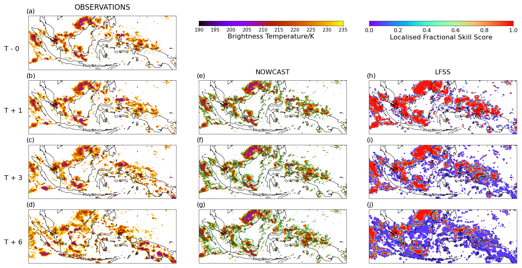
Figure 3Panels (a–d) are maps of BT observations showing convection propagating across the MC on 11 December 2019 starting from the initial observation at 09:00 LT (T−0), followed by the observation at 1 h (T + 1), 3 h (T + 3) and 6 h (T + 6) later. Panels (e–g) are the nowcasts produced by the LK algorithm at each of the corresponding observations, and the green lines show the contour of the corresponding persistence nowcast. Panels (h–j) are the LFSS maps produced by evaluating each nowcast against the corresponding observation on a 20 km spatial scale.
3.1 Deterministic nowcasting – Lucas–Kanade algorithm
Figure 3e–g show an example of a nowcast (each lead time is produced using the same T−0, T−1 and T−2 observations) produced by the LK algorithm for a qualitative assessment of the skill against observations (Fig. 3a–d), whilst Fig. 3h–j provides the LFSS (evaluated on a 20 km scale to show clearly defined differences in skill) at each time step of the nowcast (where Nt=1) for a quantitative assessment. This particular set of observations contains convection on a range of scales, with regions of propagation and regions of initiation, providing a good example to evaluate the LK algorithm on a range of capabilities (for this reason the same example is used throughout the paper). At T−0, the observed organised, large-scale convection (e.g. north of Borneo) approximately maintains its shape through T + 1 and T + 3 and then starts to change in structure at T + 6 (e.g. east of Sumatra). There is also the development of relatively smaller-scale convection observed during the T + 3 and T + 6 h lead times (e.g. over New Guinea).
Visually, the deterministic LK approach appears to predict the propagation of large-scale, organised convection well. The T + 1 nowcast best resembles the corresponding observation due to the least amount of new convection developing during this time, as well as little propagation of the organised convection (the nowcast at T + 1 closely matches the persistence nowcast). This is seen in Fig. 3h, which shows high skill in the organised convective regions over the majority of the domain. As the lead time increases, westward propagation of the large-scale convection is observed, which appears to be effectively tracked by the LK nowcast at T + 3 (e.g. east of Sumatra). This is confirmed in Fig. 3i, which shows the skill of the nowcast at T + 3 remaining high over the regions of organised convection. There is, however, a clear increase in areas of low skill at T + 3 and T + 6 due to the LK nowcast being unable to reproduce the IGD of convection. At T + 6, the change in structure of convection also contributes to the majority of the domain experiencing low skill. The nowcast at this lead time shows the least resemblance to the observations with only the largest regions of predicted convection providing any skill (Fig. 3j).
Figure 3 highlights some of the key advantages and disadvantages of the LK algorithm. Overall, it does well at predicting the propagation of large-scale, organised convection. However, because of the principle that underlies optical flow – that each pixel maintains its intensity between time steps – it is unable to capture the IGD of convection. Smaller-scale convection exhibits higher rates of change in its evolution (Venugopal et al., 1999) and so has the greatest uncertainty associated with it. Initially, this justifies why the majority of low skill is seen at smaller scales (Fig. 3h-i). However, at T + 6 the difference in small-scale features between the observations and the nowcast becomes more widespread, and so the low skill spreads further across the domain (Fig. 3j).
Figure 4 shows the mean FSSs for all 3467 LK nowcasts (Table 2) and their corresponding persistence nowcasts, evaluated at spatial scales of 10, 20, 60, 100 and 200 km. The 10 km spatial scale is the smallest scale of evaluation; hence it consistently produces the lowest scores. However, the model still shows good skill on this scale (FSS≥0.5) at a lead time of 4 h. Doubling the spatial scale to 20 km increases the skilful lead time by ∼ 1 h. At the 60, 100 and 200 km spatial scales, the LK nowcasts show skill across all lead times with FSS scores of ∼ 0.54, ∼ 0.61 and ∼ 0.75, respectively, at the 6 h lead time.
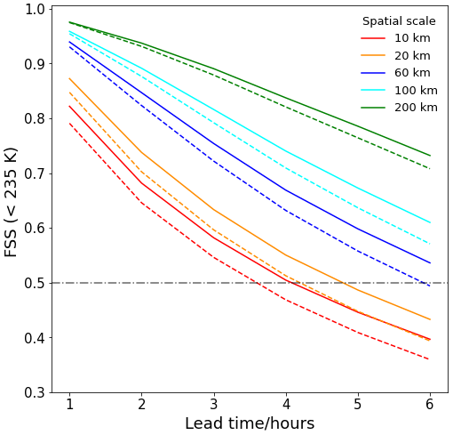
Figure 4Composite FSSs against lead time for 3457 LK nowcasts (solid line) and persistence nowcasts (dashed line), evaluated at a threshold of 235 K for 20, 50, 60, 100 and 200 km spatial scales. The grey horizontal line marks the 0.5 FSS line, which is considered the cut-off for nowcast skill.
Skill reduces with lead time for all spatial scales and increases with spatial scale at all lead times. On average, the LK nowcasts outperform the persistence nowcasts at all lead times and for all spatial scales. Both the persistence and the LK nowcasts maintain the same structure and intensity at each lead time (hence relatively smaller skill difference at 1–2 h lead time). However, the LK nowcasts propagate the convection across the domain, whereas the persistence nowcasts remain stationary. This explains the increasing added value of the LK nowcast with lead time, as the observations move further from the persistence nowcast and the skill difference increases. Greater added value of the LK nowcast over persistence is also seen at smaller spatial scales. For example, the skill gap between the persistence nowcasts and the LK nowcasts at the 6 h lead time is greater for 10 km spatial scale compared to 200 km spatial scale. The trend of FSSs across the shown lead times also varies for different spatial scales. At smaller spatial scales the nowcast is being evaluated on its ability to predict smaller-scale convection, which changes most rapidly/unpredictably, resulting in a higher rate of decrease in skill. The FSS evaluation on higher spatial scales smooths out these smaller-scale convection changes, and so a much lower rate of decrease in skill is seen. The rate of decrease of the FSS evaluated on the 10 km spatial scale appears to show its largest rate of skill decrease at 1–2 h and then decelerates over the following time intervals. On the other hand the rate of skill decrease for the 200 km spatial scale increases with lead time.
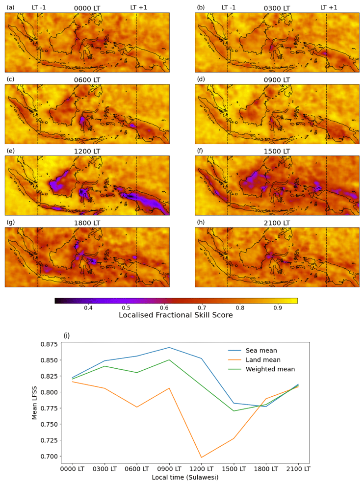
Figure 5(a–g) Composite LFSS maps for 3 h lead time nowcasts that were initialised at 00:00 LT, 03:00 LT, 09:00 LT, 12:00 LT, 15:00 LT, 18:00 LT and 21:00 LT, respectively. The LFSS was evaluated on a 100 km scale, and the local time is with reference to Sulawesi (the vertical dotted lines show the time difference across the domain). (i) The mean LFSSs at each initialisation time for sea only, land only and the whole domain.
Figure 5 shows the mean LFSS for 3 h lead time nowcasts over the MC, evaluated at a 100 km spatial scale. Evaluation on this scale has been used as it is able to clearly highlight the variations of skill across the domain. For all nowcast initialisation times there is consistent noise in the skill over the sea. This may be representative of the stochastic nature of convection initiation over the sea. It therefore would be expected that, if the period of evaluation were extended beyond 2015–2020 (i.e. increasing the number of nowcasted events used in the averaging over time in Eqs. 8 and 9), the LFSS noise field would become smoother over the sea. During the overnight and morning initialisation times (Fig. 5a–d) there is, on average, high skill over the majority of the domain (Fig. 5i). This is to be expected as at these times the majority of convection has formed large-scale, organised cloud systems with very few small-scale convection initiations occurring. These larger-scale systems will most often be propagating offshore of the islands (as part of the diurnal cycle), which the LK algorithm is most effective at capturing. Furthermore, overnight and during the morning there is, on average, relatively less convective activity than during the day meaning that reduced skill from inaccurate propagation predictions is minimised.
Between 09:00 LT and 12:00 LT there is a significant drop in the mean skill over land (Fig. 5i). Figure 5e–f show these distinct regions of low skill over land, which are tightly constrained to the coastal and mountainous regions of the islands and are closely tied to the diurnal cycle of convection over the MC. Convection begins to initiate and develop over the coastal and mountainous regions of the islands in the early afternoon, which is not present at 12:00 LT. The LK nowcast is unable to capture this new convection, resulting in low overland skill for the 12:00 LT initialisation. Over these locations at this time of day, the LK algorithm would not be a skilful nowcasting tool. The low skill is still seen at 15:00 LT but to a lesser extent. At this initialisation time the T−0 observations that are inputted into the LK algorithm will, on average, contain the majority of the convection that has initiated over the early afternoon. This convection will likely remain stationary over this time but will be growing in size. Therefore the persisting low skill at 15:00 LT is representative of the LK nowcasts' inability to predict the growth of convection.
The development of convection starts to slow as storms reach their mature stage in the evening. Less growth results in higher skill over the land. At 21:00 LT the LFSS map looks similar to the overnight LFSS maps with high skill across the entire domain. Over this 3 h forecast period the LK algorithm has shown good skill at being able to nowcast the propagation of mesoscale convective systems offshore, which developed overland during the afternoon.
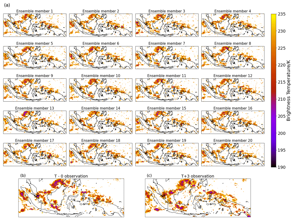
Figure 6(a) An example of a 20-member ensemble, 3 h lead time BT nowcast produced by the STEPS implementation of pySTEPS on 11 December 2019. (b) The observation at the nowcast initialisation time and (c) the observation 3 h later.
Understanding that the LK algorithm is unable to predict the IGD of convection means that, by identifying anomalous regions of low skill, LFSS maps can be a useful tool for identifying local effects due to land–sea interactions. An example of this is seen in a region of low skill over the northeast coast of Borneo at 18:00 LT. On average, at this time of the day a land breeze begins to develop along the entire concave-shaped coastline, potentially causing convergence near the middle. This convergence may then lead to the initiation of convection that the LK algorithm is unable to predict.
3.2 Ensemble nowcasting – STEPS algorithm
Figure 6a provides an example of a 20-member ensemble nowcast (generated using the same T−2, T−1 and T−0 set as for the LK algorithm example in Fig. 3), with a lead time of 3 h, produced by pySTEPS's implementation of STEPS. Over the 3 h period the main differences between the T−0 and T + 3 observations are around New Guinea where new convection develops over the land and the convection north of the island becomes more scattered (Fig. 6b–c). Visually, each ensemble member provides a good prediction of the large-scale convection (e.g. north of Borneo), with little difference between the members in the predicted shape and structure. The main differences between the ensemble members come from differences in the stochastic fields injected for each member. This is seen in the varying levels of BT intensities in the large-scale convection in each member. For example, the BT intensity over northern Borneo in ensemble member 13 is greater than in ensemble member 2. Differences are also seen between each ensemble member in the distribution of the predicted small-scale convection (e.g. over the Philippine Sea). Over Borneo, some members have predicted small-scale convection which approximately aligns with the new convection observed at T + 3 (e.g. ensemble member 18), whereas some members have predicted no convection here at all (e.g. ensemble member 17).
One of the key aims of STEPS is to address the uncertainty in the evolution of small-scale convection. In all members the convection northwest of New Guinea appears much noisier than in the T−0 observation. STEPS has recognised this as a region of uncertainty and addressed it by injecting noise at this scale. When compared to the T + 3 observation, it can be seen that the convection does in fact become more scattered and dissipated, and so, although STEPS has not been able to precisely predict the new shape of the scattered convection, it has been able to capture the unpredictable nature of the evolution of this small-scale convection.
The 20-member ensemble in Fig. 6 has been used to produce the probabilistic nowcast in Fig. 7 (extended to 1, 3 and 6 h lead times). This probabilistic nowcast uses a threshold of 235 K, therefore including all the pixels that were used to produce each ensemble nowcast. At T + 1 the probabilistic nowcast shows a high degree of certainty in its prediction of the shape and location of convection, meaning that there is little variance between ensemble members. The T + 1 lead time is the first time step prediction that the algorithm makes, and so it contains the least amount of stochastic noise in the extrapolation motion field, hence the least amount of member variance. As the lead time increases, more stochastic noise is injected into the extrapolation motion fields, and so the uncertainty of the probabilistic nowcast increases. This can be seen in the reduction in high probabilities over the regions enclosed within the 20 % contour. A reduction of high uncertainties within the 20 % contour is also matched with a greater spread of low ensemble probability across the entire domain (outside the 20 % contour) at T + 3 and T + 6.
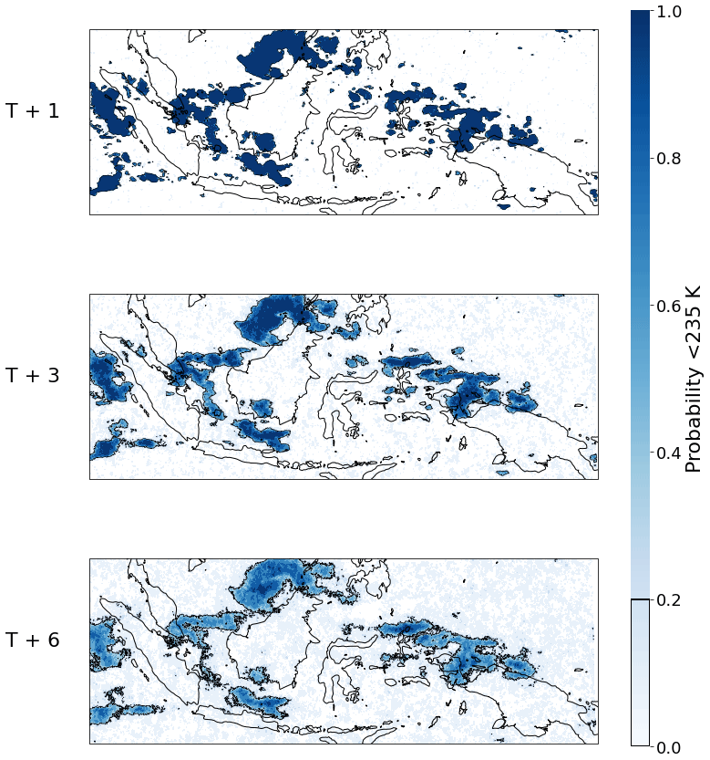
Figure 7An example of a probabilistic BT nowcast for lead times of 1, 3 and 6 h produced by the STEPS implementation of pySTEPS on 11 December 2019. A BT threshold of < 235 K is used in order to include all pixels in the nowcast.
Figure 7 also shows the number of small-scale features in the probabilistic nowcast reducing at longer lead times. For example, at T + 1 the convection northwest of New Guinea appears scattered in small blobs, whereas at T + 6 STEPS has smoothed out this small-scale convection into a larger region. Again, this is evidence of the algorithm's attempt to address the uncertainty in the evolution of small-scale convection by replacing it with stochastic noise.
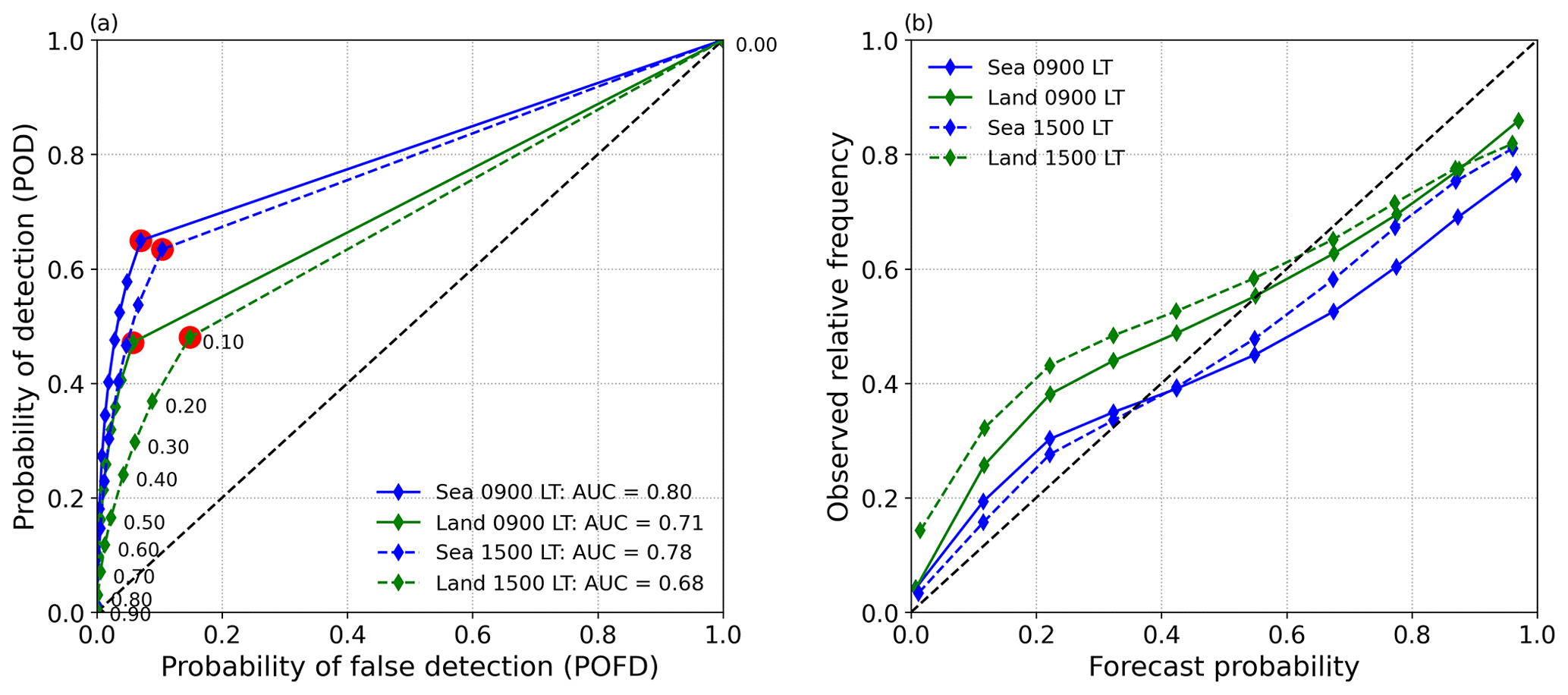
Figure 8Composite (a) ROC and (b) reliability curves over the sea and land for STEPS 3 h lead time nowcasts, initialised at 09:00 (441 nowcasts) and 15:00 (405 nowcasts), with a threshold of < 235 K. The numbers next to the green points in (a) represent the thresholds used to evaluate the nowcast at different likelihoods. Red dot represents the optimum threshold.
Figure 8a and b show the mean ROC and reliability curves for STEPS nowcasts initialised in the morning (09:00 LT) and afternoon (15:00 LT), evaluated over the sea and the land. For both surface types and initialisation times, the POD increases at each threshold meaning that, even as more uncertain regions enter the evaluation, the proportion of hits to misses increases. Furthermore, the POD exceeds the POFD at each threshold indicating that STEPS has skill in predicting regions < 235 K BT over the MC. The greatest POD–POFD difference, which is considered the optimum threshold for a probabilistic nowcast, is shown at the ≥ 10 % likelihood threshold for all of the curves.
For both initialisation times in Fig. 8a, STEPS produces higher area under the curve (AUC) scores over the sea (0.80 and 0.78 for 09:00 LT and 15:00 LT, respectively) than over the land (0.71 and 0.68 for 09:00 LT and 15:00 LT, respectively), meaning that STEPS has more skill over the sea at these times. This can be explained by lower POD scores over the land, which is due to the STEPS algorithm being unable to capture the new convection that most often develops there (increasing the number of misses). Furthermore, a comparison of each region within initialisation times suggests that STEPS is slightly more skilful in the morning (average AUC of 0.76) than in the afternoon (average AUC of 0.73). The morning–afternoon difference in POFD is also much greater over the land than the sea. This is likely due to a greater decrease in correct negative scores over the land, caused by new convection initiating where there was previously none, which STEPS is unable to predict.
The positive slope between all the points for each reliability curve in Fig. 8b means that, over both surface types, as the observed frequency of events increases, STEPS predicts a higher likelihood of that event occurring. This shows that overall STEPS is able to produce a reliable nowcast for these initialisation times. However, for both regions and times of day, STEPS presents a lower probability than the observed frequency for probabilities ≲ 0.35 and a higher probability than the observed frequency for probabilities ≳ 0.65. The distribution of ensemble predictions is therefore under-dispersive, meaning that the spread of predictions falls within the spread of observations; i.e. it does not provide an optimum estimate of uncertainty.
When comparing the two surface types it can be seen that the under-prediction at lower nowcast probabilities is greater over the land, meaning the ensemble distribution has less variance and STEPS is better at capturing uncertainty over the sea for these initialisation times. However, at higher nowcast probabilities, more over-prediction is seen over the sea compared to over the land, meaning that STEPS becomes too confident at predicting higher-likelihood events over the sea.
The under-dispersive feature of STEPS over the MC is due to low ensemble member variance, which (as previously mentioned) can be exemplified by visually assessing the lack of diversity between the ensemble members in Fig. 6. The main source of ensemble member variance comes from the differences in the stochastic noise fields that STEPS injects into the nowcasts, and so, increasing the range of noise field intensities, or simply adding more members, would likely help to reduce this under-dispersive feature.
3.3 Comparison of STEPS, LK and persistence
By applying a threshold to a probabilistic STEPS nowcast, it is possible to produce a deterministic STEPS nowcast (in the form of a binary field) that can be evaluated using the FSS and directly compared to the corresponding LK and persistence nowcast. Figure 9 shows the mean FSSs for 3467 LK nowcasts (solid), persistence nowcasts (dashed) and STEPS deterministic nowcasts produced using a threshold of ≥ 10 % (dotted; STEPS10). The choice of threshold was based on the results of Fig. 8, which show that, for both the morning and evening initialisation times, the optimum likelihood threshold was ≥ 10 %.
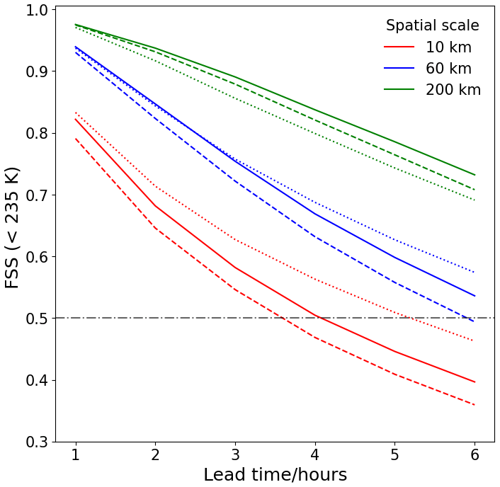
Figure 9Composite FSSs against lead time for 3457 LK (solid line), STEPS10 (dotted line) and persistence (dashed line) nowcasts, evaluated at a threshold of 235 K for 10, 60 and 200 km spatial scales. The grey horizontal line marks the 0.5 FSS line, which is considered the cut-off for nowcast skill.
At 10 km spatial scale, STEPS10 shows skill up to ∼ 5 h and has the highest skill across all lead times, outperforming LK and persistence. At 60 km scales STEPS10 still outperforms persistence across all lead times but approximately equals the skill of LK from 1–3 h lead time. Onwards of 3 h lead time, STEPS10 shows higher skill than LK.
The added value of STEPS10 over both LK and persistence decreases between the 10 and 60 km spatial scales and, by the 200 km scale, STEPS10 shows the least skill out of all the nowcasts. This is likely due to less of the propagation being detected within the 200 km scale evaluation compared to the 10 and 60 km scales – hence LK tends towards persistence at greater scales. Unlike LK, STEPS changes the internal structure of the convection through the injection of stochastic noise. This change in the internal structure of convection (as opposed to change due to propagation) will be detected on the 200 km spatial scale and may contribute to a drop in performance relative to LK and persistence.
A deterministic (LK algorithm) and probabilistic (STEPS algorithm) implementation of the pySTEPS optical flow nowcasting library have been applied to satellite data over the MC to produce nowcasts with lead times of up to 6 h.
Overall, the LK algorithm predicts the propagation of convection across the domain with skill (FSS ≥ 0.5) up to 4 h on the 10 km scale (the smallest scale of evaluation) and up to at least 6 h on the 60 km scale. Similarly, Burton et al. (2022) used the LK algorithm to nowcast convective rain rates over West Africa using retrievals of BTs. Although it is difficult to precisely compare the two sets of results (rainfall retrievals likely have more fine-scale variability and errors in rainfall retrievals will affect nowcast skill (Hill et al., 2020)) they are nevertheless comparable. Burton et al. (2022) show skill up to about 3 h on the 64 km scale, whereas we would expect somewhat higher skill for BT nowcasts over the MC.
Similar to the findings in Burton et al. (2022), the LK algorithm was unable to predict the initiation–growth–decay of convection, which is a manifestation of the optical flow assumption – each pixel maintains its intensity across all time steps. This inability to predict IGD of convection is clearly seen when analysing maps of LFSS over the MC. Over the sea the LK algorithm shows, on average, good skill at all nowcast initialisation times due to convection being mostly propagating in nature. Over land, however, the model shows high skill in the morning and evening but much lower skill in the afternoon. In the early afternoon this is due to the initiation of convection, which is closely constrained to the mountains. Later in the afternoon the low skill is due to the growth of the convection that initiated earlier on and persists over the mountains. Over the mountainous regions of the MC during the afternoon, the LK algorithm would not be a useful nowcasting tool.
The STEPS algorithm aims to address the issue of unpredictability in the initiation–growth–decay of convection by injecting varying intensities of stochastic noise at different length scales to produce an ensemble nowcast. When analysing a probabilistic nowcast produced by a STEPS ensemble, it can be seen that the injection of noise has a smoothing effect, removing small-scale convection and maintaining the shape of the larger, more predictable convective regions.
A composite analysis of STEPS nowcasts was performed using ROC and reliability curves for 3 h lead times predictions. The ROC curve is a measure of a nowcast's ability to discriminate between convective events that happened and convective events that did not (the higher the area under a ROC curve, the more efficient it is at this), whereas the reliability curve measures how well the probabilistic predictions compare to observations. Overall, the analysis showed that STEPS can produce both skilful and reliable ensemble predictions for 3 h lead times. When comparing land and sea at different times of day, it was shown that STEPS has highest skill over the sea during the morning (09:00 LT initialisation time) with an AUC score of 0.8 (compared to an AUC score of 0.71 over the land). Imhoff et al. (2020) also applied the pySTEPS implementation of STEPS to radar data over the Netherlands to produce nowcasts for a range of lead times. In their work they produced composite ROC curves for nowcasts with a lead time of 95–120 min, which had an AUC score of 0.81. The Netherlands experiences far less convective activity than the MC with the majority of its weather coming from propagating frontal clouds. This, therefore, further highlights the effectiveness of STEPS for the MC as it tries to predict convective clouds, which have a more unpredictable nature. However, the disadvantages of STEPS were revealed when analysing the reliability curves. A common feature across both times and regions was the under-dispersive ensemble distributions, which were more extreme over land. This highlights STEPS's inability to predict the low-likelihood events (e.g. new initiations) and capture the whole uncertainty of the observed system.
To compare STEPS with LK and persistence, a deterministic version of STEPS was produced by thresholding the probabilistic nowcasts at ≥ 10 % (STEPS10). When evaluated, the STEPS10 nowcasts had higher skill at spatial scales of 10 km (across all lead times) and 60 km (from 3–6 h). Therefore, not only does STEPS provide insight into the uncertainty of a convective system, but it can also derive a better single deterministic nowcast than LK and persistence at these scales. However, at a higher spatial scale of 200 km (where relatively less convection propagation is detected), LK nowcasts had the highest overall skill and the injection of stochastic noise produced by STEPS likely caused the STEPS10 nowcasts to have the lowest overall skill.
Continuous nowcasting over the entire MC is a requirement for early-warning systems, which does not currently exist. By providing both nowcast examples and composite nowcast analysis, this paper has shown the effective application of a deterministic (LK) and probabilistic (STEPS) algorithm to satellite data, showing their potential to be used operationally over the whole of the MC. The work highlights the key strengths and weaknesses of both algorithms, providing important information to a potential forecaster using these tools.
Code is available from the first author upon request.
Himawari data are available from the ICARE Data and Services Center at the University of Lille, at https://www.icare.univ-lille1.fr (University of Lille, 2024).
JS performed the analysis and wrote the paper. CB, JM and SP participated in technical discussions and provided guidance for the analysis. MB and GP provided guidance for writing the paper.
The contact author has declared that none of the authors has any competing interests.
Publisher's note: Copernicus Publications remains neutral with regard to jurisdictional claims made in the text, published maps, institutional affiliations, or any other geographical representation in this paper. While Copernicus Publications makes every effort to include appropriate place names, the final responsibility lies with the authors.
The author would like to acknowledge the SENSE CDT for providing the technical training for this project.
This paper was edited by Vassiliki Kotroni and reviewed by two anonymous referees.
Ali, A., Supriatna, S., and Sa'adah, U.: Radar-Based Stochastic Precipitation Nowcasting Using The Short-Term Ensemble Prediction System (STEPS) (Case Study: Pangkalan Bun Weather Radar), International Journal of Remote Sensing and Earth Sciences, 18, 91, https://doi.org/10.30536/j.ijreses.2021.v18.a3527, 2021.
Ayzel, G., Scheffer, T., and Heistermann, M.: RainNet v1.0: a convolutional neural network for radar-based precipitation nowcasting, Geosci. Model Dev., 13, 2631–2644, https://doi.org/10.5194/gmd-13-2631-2020, 2020.
Bessho, K., Date, K., Hayashi, M., Ikeda, A., Imai, T., Inoue, H., Kumagai, Y., Miyakawa, T., Murata, H., Ohno, T., Okuyama, A., Oyama, R., Sasaki, Y., Shimazu, Y., Shimoji, K., Sumida, Y., Suzuki, M., Taniguchi, H., Tsuchiyama, H., Uesawa, D., Yokota, H., and Yoshida, R.: An Introduction to Himawari-8/9 — Japan's New-Generation Geostationary Meteorological Satellites, J. Meteorol. Soc. Jpn., 94, 151–183, https://doi.org/10.2151/jmsj.2016-009, 2016.
Birch, C. E., Webster, S., Peatman, S. C., Parker, D. J., Matthews, A. J., Li, Y., and Hassim, M. E. E.: Scale Interactions between the MJO and the Western Maritime Continent, J. Climate, 29, 2471–2492, https://doi.org/10.1175/JCLI-D-15-0557.1, 2016.
Bowler, N. E., Pierce, C. E., and Seed, A. W.: STEPS: A probabilistic precipitation forecasting scheme which merges an extrapolation nowcast with downscaled NWP, Q. J. Roy. Meteor. Soc., 132, 2127–2155, https://doi.org/10.1256/qj.04.100, 2006.
Burton, R. R., Blyth, A. M., Cui, Z., Groves, J., Lamptey, B. L., Fletcher, J. K., Marsham, J. H., Parker, D. J., and Roberts, A.: Satellite-based nowcasting of West African mesoscale storms has skill at up to four hours lead time, Weather Forecast., 37, 445–455, https://doi.org/10.1175/WAF-D-21-0051.1, 2022.
Dayem, K. E., Noone, D. C., and Molnar, P.: Tropical western Pacific warm pool and maritime continent precipitation rates and their contrasting relationships with the Walker Circulation, J. Geophys. Res., 112, D06101, https://doi.org/10.1029/2006JD007870, 2007.
Feng, Z., Leung, L. R., Liu, N., Wang, J., Houze, R. A., Li, J., Hardin, J. C., Chen, D., and Guo, J.: A Global High-Resolution Mesoscale Convective System Database Using Satellite-Derived Cloud Tops, Surface Precipitation, and Tracking, J. Geophys. Res.-Atmos., 126, e2020JD034202, https://doi.org/10.1029/2020JD034202, 2021.
Ferrett, S., Frame, T. H. A., Methven, J., Holloway, C. E., Webster, S., Stein, T. H. M., and Cafaro, C.: Evaluating convection-permitting ensemble forecasts of precipitation over Southeast Asia, Weather Forecast., 36, 1199–1217, https://doi.org/10.1175/WAF-D-20-0216.1, 2021.
Germann, U. and Zawadzki, I.: Scale-Dependence of the Predictability of Precipitation from Continental Radar Images. Part I: Description of the Methodology, Mon. Weather Rev., 130, 2859–2873, https://doi.org/10.1175/1520-0493(2002)130<2859:SDOTPO>2.0.CO;2, 2002.
Gijben, M. and de Coning, E.: Using Satellite and Lightning Data to Track Rapidly Developing Thunderstorms in Data Sparse Regions, Atmosphere, 8, 67, https://doi.org/10.3390/atmos8040067, 2017.
Haiden, T., Kann, A., Wittmann, C., Pistotnik, G., Bica, B., and Gruber, C.: The Integrated Nowcasting through Comprehensive Analysis (INCA) System and Its Validation over the Eastern Alpine Region, Weather Forecast., 26, 166–183, https://doi.org/10.1175/2010WAF2222451.1, 2011.
Han, D., Lee, J., Im, J., Sim, S., Lee, S., and Han, H.: A Novel Framework of Detecting Convective Initiation Combining Automated Sampling, Machine Learning, and Repeated Model Tuning from Geostationary Satellite Data, Remote Sens.-Basel, 11, 1454, https://doi.org/10.3390/rs11121454, 2019.
Han, L., Zhang, J., Chen, H., Zhang, W., and Yao, S.: Toward the Predictability of a Radar-Based Nowcasting System for Different Precipitation Systems, IEEE Geosci. Remote S., 19, 1–5, https://doi.org/10.1109/LGRS.2022.3185031, 2022.
Harjupa, W., Abdillah, M. R., Azura, A., Putranto, M. F., Marzuki, M., Nauval, F., Risyanto, Saufina, E., Jumianti, N., and Fathrio, I.: On the utilization of RDCA method for detecting and predicting the occurrence of heavy rainfall in Indonesia, Remote Sensing Applications: Society and Environment, 25, 100681, https://doi.org/10.1016/j.rsase.2021.100681, 2022.
Hill, P. G., Stein, T. H. M., Roberts, A. J., Fletcher, J. K., Marsham, J. H., and Groves, J.: How skilful are Nowcasting Satellite Applications Facility products for tropical Africa?, Meteorol. Appl., 27, 12, https://doi.org/10.1002/met.1966, 2020.
Horn, B. K. P. and Schunck, B. G.: Determining optical flow, Artif. Intell., 17, 185–203, https://doi.org/10.1016/0004-3702(81)90024-2, 1981.
Hou, A. Y., Kakar, R. K., Neeck, S., Azarbarzin, A. A., Kummerow, C. D., Kojima, M., Oki, R., Nakamura, K., and Iguchi, T.: The Global Precipitation Measurement Mission, B. Am. Meteorol. Soc., 95, 701–722, https://doi.org/10.1175/BAMS-D-13-00164.1, 2014.
Imhoff, R. O., Brauer, C. C., Overeem, A., Weerts, A. H., and Uijlenhoet, R.: Spatial and Temporal Evaluation of Radar Rainfall Nowcasting Techniques on 1,533 Events, Water Resour. Res., 56, e2019WR026723, https://doi.org/10.1029/2019WR026723, 2020.
Lagerquist, R., Stewart, J., Ebert-Uphoff, I., and Christina, K.: Using Deep Learning to Nowcast the Spatial Coverage of Convection from Himawari-8 Satellite Data, Mon. Weather Rev., 149, 3897–3921, https://doi.org/10.1175/MWR-D-21-0096.1, 2021.
Lebedev, V., Ivashkin, V., Rudenko, I., Ganshin, A., Molchanov, A., Ovcharenko, S., Grokhovetskiy, R., Bushmarinov, I., and Solomentsev, D.: Precipitation Nowcasting with Satellite Imagery, in: Proceedings of the 25th ACM SIGKDD International Conference on Knowledge Discovery & Data Mining, KDD '19, 25 July 2019, Anchorage, AK, USA, 2680–2688, https://doi.org/10.1145/3292500.3330762, 2019.
Line, W. E., Schmit, T. J., Lindsey, D. T., and Goodman, S. J.: Use of Geostationary Super Rapid Scan Satellite Imagery by the Storm Prediction Center, Weather Forecast., 31, 483–494, https://doi.org/10.1175/WAF-D-15-0135.1, 2016.
Lucas, B. D. and Kanade, T.: An Iterative Image Registration Technique with an Application to Stereo Vision, 10, in: Proceedings: 7th international joint conference on Artificial intelligence – Volume 2, Morgan Kaufmann Publishers Inc., San Francisco, CA, USA, https://dl.acm.org/doi/10.5555/1623264.1623280 (last access: 14 February 2024), 1981.
Machado, L. A. T. and Laurent, H.: The Convective System Area Expansion over Amazonia and Its Relationships with Convective System Life Duration and High-Level Wind Divergence, Mon. Weather Rev., 132, 714–725, https://doi.org/10.1175/1520-0493(2004)132<0714:TCSAEO>2.0.CO;2, 2004.
Marcos: NWC SAF convective precipitation product from MSG: A new day-time method based on cloud top physical properties, Tethys, 12, 3–11, https://doi.org/10.3369/tethys.2015.12.01, 2015.
Mori, S., Jun-Ichi, H., Tauhid, Y. I., Yamanaka, M. D., Okamoto, N., Murata, F., Sakurai, N., Hashiguchi, H., and Sribimawati, T.: Diurnal Land–Sea Rainfall Peak Migration over Sumatera Island, Indonesian Maritime Continent, Observed by TRMM Satellite and Intensive Rawinsonde Soundings, Mon. Weather Rev., 132, 2021–2039, https://doi.org/10.1175/1520-0493(2004)132<2021:DLRPMO>2.0.CO;2, 2004.
Mueller, C., Saxen, T., Roberts, R., Wilson, J., Betancourt, T., Dettling, S., Oien, N., and Yee, J.: NCAR Auto-Nowcast System, Weather Forecast., 18, 545–561, https://doi.org/10.1175/1520-0434(2003)018<0545:NAS>2.0.CO;2, 2003.
Murphy, A. H. and Epstein, E. S.: Skill Scores and Correlation Coefficients in Model Verification, Mon. Weather Rev., 117, 572–582, https://doi.org/10.1175/1520-0493(1989)117<0572:SSACCI>2.0.CO;2, 1989.
Permana, D. S., Hutapea, T. D., Praja, A. S., Paski, J. A. I., Makmur, E. E. S., Haryoko, U., Umam, I. H., Saepudin, M., and Adriyanto, R.: The Indonesia In-House Radar Integration System (InaRAISE) of Indonesian Agency for Meteorology Climatology and Geophysics (BMKG): Development, Constraint, and Progress, IOP Conf. Ser.-Earth Environ. Sci., 303, 012051, https://doi.org/10.1088/1755-1315/303/1/012051, 2019.
Porson, A. N., Hagelin, S., Boyd, D. F. A., Roberts, N. M., North, R., Webster, S., and Lo, J. C.: Extreme rainfall sensitivity in convective-scale ensemble modelling over Singapore, Q. J. Roy. Meteor. Soc., 145, 3004–3022, https://doi.org/10.1002/qj.3601, 2019.
Pulkkinen, S., Nerini, D., Pérez Hortal, A. A., Velasco-Forero, C., Seed, A., Germann, U., and Foresti, L.: Pysteps: an open-source Python library for probabilistic precipitation nowcasting (v1.0), Geosci. Model Dev., 12, 4185–4219, https://doi.org/10.5194/gmd-12-4185-2019, 2019.
Qian, J.-H.: Why Precipitation Is Mostly Concentrated over Islands in the Maritime Continent, J. Atmos. Sci., 65, 1428–1441, https://doi.org/10.1175/2007JAS2422.1, 2008.
Ramage, C. S.: ROLE OF A TROPICAL “MARITIME CONTINENT” IN THE ATMOSPHERIC CIRCULATION, Mon. Weather Rev., 96, 365–370, https://doi.org/10.1175/1520-0493(1968)096<0365:ROATMC>2.0.CO;2, 1968.
Reen, B. P., Cai, H., and Raby, J. W.: Preliminary Investigation of Assimilating Global Synthetic Weather Radar, United States Army Research Lab., https://apps.dtic.mil/sti/pdfs/AD1111072.pdf (last access: 14 February 2024), 2020.
Roberts, A. J., Fletcher, J. K., Groves, J., Marsham, J. H., Parker, D. J., Blyth, A. M., Adefisan, E. A., Ajayi, V. O., Barrette, R., de Coning, E., Dione, C., Diop, A., Foamouhoue, A. K., Gijben, M., Hill, P. G., Lawal, K. A., Mutemi, J., Padi, M., Popoola, T. I., Rípodas, P., Stein, T. H. M., and Woodhams, B. J.: Nowcasting for Africa: advances, potential and value, Weather, 77, 250–256, https://doi.org/10.1002/wea.3936, 2022.
Roberts, N. M. and Lean, H. W.: Scale-Selective Verification of Rainfall Accumulations from High-Resolution Forecasts of Convective Events, Mon. Weather Rev., 136, 78–97, https://doi.org/10.1175/2007MWR2123.1, 2008.
Roca, R., Fiolleau, T., and Bouniol, D.: A Simple Model of the Life Cycle of Mesoscale Convective Systems Cloud Shield in the Tropics, J. Climate, 30, 4283–4298, https://doi.org/10.1175/JCLI-D-16-0556.1, 2017.
Rouault, E., Warmerdam, F., Schwehr, K., Kiselev, A., Butler, H., Łoskot, M., Szekeres, T., Tourigny, E., Landa, M., Miara, I., Elliston, B., Chaitanya, K., Plesea, L., Morissette, D., Jolma, A., Dawson, N., Baston, D., de Stigter, C., and Miura, H.: GDAL, Zenodo [code], https://doi.org/10.5281/ZENODO.5884351, 2023.
Seed, A. W.: A Dynamic and Spatial Scaling Approach to Advection Forecasting, J. Appl. Meteorol., 42, 381–388, https://doi.org/10.1175/1520-0450(2003)042<0381:ADASSA>2.0.CO;2, 2003.
Shi, J. and Tomasi: Good features to track, in: Proceedings of IEEE Conference on Computer Vision and Pattern Recognition CVPR-94, 21–23 June 1994, Seattle, WA, USA, 593–600, https://doi.org/10.1109/CVPR.1994.323794, 1994.
Sieglaff, J. M., Hartung, D. C., Feltz, W. F., Cronce, L. M., and Lakshmanan, V.: A Satellite-Based Convective Cloud Object Tracking and Multipurpose Data Fusion Tool with Application to Developing Convection, J. Atmos. Ocean. Tech., 30, 510–525, https://doi.org/10.1175/JTECH-D-12-00114.1, 2013.
Sobajima, A.: Rapidly Developing Cumulus Areas Derivation Algorithm Theoretical Basis Document, Japanese Meteorological Agency, https://cwg.eumetsat.int/res/pdf/ATBD_RapidlyDevelopingCumulusAreas_CWG.pdf (last access: 14 February 2024), 2012.
Srivastava, K., Lau, Sharons. Y., Yeung, H. Y., Cheng, T. L., Bhardwaj, R., Kannan, A. M., Bhowmik, S. K. R., and Singh, H.: Use of SWIRLS nowcasting system for quantitative precipitation forecast using Indian DWR data, MAUSAM, 63, 1–16, https://doi.org/10.54302/mausam.v63i1.1442, 2021.
University of Lille: ICARE Data and Services Center, https://www.icare.univ-lille.fr/ (last access: 13 February 2024), 2024.
Venugopal, V., Foufoula-Georgiou, E., and Sapozhnikov, V.: Evidence of dynamic scaling in space-time rainfall, J. Geophys. Res., 104, 31599–31610, https://doi.org/10.1029/1999JD900437, 1999.
Vila, D. A., Machado, L. A. T., Laurent, H., and Velasco, I.: Forecast and Tracking the Evolution of Cloud Clusters (ForTraCC) Using Satellite Infrared Imagery: Methodology and Validation, Weather Forecast., 23, 233–245, https://doi.org/10.1175/2007WAF2006121.1, 2008.
Woodhams, B. J., Birch, C. E., Marsham, J. H., Bain, C. L., Roberts, N. M., and Boyd, D. F. A.: What Is the Added Value of a Convection-Permitting Model for Forecasting Extreme Rainfall over Tropical East Africa?, Mon. Weather Rev., 146, 2757–2780, https://doi.org/10.1175/MWR-D-17-0396.1, 2018.
World Meteorological Organization: Early Warnings For All Initiative scaled up into action on the ground, World Meteorological Organization, https://wmo.int/site/wmo-and-early-warnings-all-initiative (last access: 13 February 2024), 2023.
Yamanaka, M. D.: Physical climatology of Indonesian maritime continent: An outline to comprehend observational studies, Atmos. Res., 178–179, 231–259, https://doi.org/10.1016/j.atmosres.2016.03.017, 2016.
Yang, G.-Y. and Slingo, J.: The Diurnal Cycle in the Tropics, Mon. Weather Rev., 129, 784–801, https://doi.org/10.1175/1520-0493(2001)129<0784:TDCITT>2.0.CO;2, 2001.