Investigation of historical severe storms and storm tides in the German Bight with century reanalysis data

Century reanalysis models offer a possibility to investigate extreme events and gain further insights into their impact through numerical experiments. This paper is a comprehensive summary of historical hazardous storm tides in the German Bight (southern North Sea) with the aim of comparing and evaluating the potential of different century reanalysis data to be used for the reconstruction of extreme water levels. The composite analysis of historical water level extremes, underlying atmospheric situations and their uncertainties may further support decision-making on coastal protection and risk assessment. The analysis is done based on the results of the regional hydrodynamic model simulations forced by atmospheric century reanalysis data, e.g. 20th Century Reanalysis Project (20CR) ensembles, ERA5 and UERRA–HARMONIE. The eight selected historical storms lead either to the highest storm tide extremes for at least one of three locations around the German Bight or to extreme storm surge events during low tide. In general, extreme storm tides could be reproduced, and some individual ensemble members are suitable for the reconstruction of respective storm tides. However, the highest observed water level in the German Bight could not be simulated with any considered forcing. The particular weather situations with corresponding storm tracks are analysed to better understand their different impact on the peak storm tides, their variability and their predictability. Storms with more northerly tracks generally show less variability in wind speed and a better agreement with the observed extreme water levels for the German Bight. The impact of two severe historical storms that peaked at low tide is investigated with shifted tides. For Husum in the eastern German Bight this results in a substantial increase in the peak water levels reaching a historical maximum.

1 Introduction

The German Bight (Fig. 1), as part of the south-eastern North Sea, is exposed to storm tides, which represent natural hazards for the low-lying coastal areas. In the last 120 years, a few severe storms occurred with partly considerable damage at the coasts of the German Bight and in the hinterland connected to the North Sea by the rivers (e.g. Ems, Weser, Elbe, Eider). One example is the storm on 16/17 February 1962 which caused extensive damage due to very high water levels in the German Bight and insufficient protection at the coast and along the rivers. After this event, coastal defences were significantly improved (e.g. higher dike line and barriers), and the storm tide on 3 January 1976, also one of the highest during the last 120 years, caused less damage mainly due to the improved protection (Kuratorium für Forschung im Küsteningenieurwesen, 1979).

Despite the extensive improvement in coastal protection along the coasts of the German Bight, the risk of flooding is still present and will increase in the future in the context of anthropogenic climate change. The observational data of water level from the tide gauges extend more than a century back in time and provide an indispensable source of information about extreme storm events and their impact on the coast. However, these measurements are sporadic by nature and for large parts of the coastline not available. The hydrodynamic models have traditionally been used as an additional tool to estimate water levels along the coastline regularly. Storm tides, causing the main flooding hazard at the coasts, can be considered a composition of atmospherically driven components like storm surge and external surge, the tidal component, and their non-linear interaction. Leaving aside the changing bathymetry, coastal outline and protection constructions, the main uncertainty in the modelling of historical storm tides originates in atmospheric forcing. Thus, the realistic reconstruction of wind and pressure fields during the storm is necessary for adequate storm tide estimations. As the observational atmospheric data over the sea are sparse and irregular, especially during the pre-satellite era, atmospheric reanalysis has appeared in the past 3 decades (e.g. NCEP–NCAR, ERA-40, ERA-Interim, ERA-20C, CERRA). These reconstructions of the atmospheric state are produced with atmospheric models, which also consider available measurements by assimilation procedures.

In recent years, more reanalysis products have become available at higher spatial and temporal resolution, improving the representation of localised effects by resolving relevant mesoscale processes (e.g. ERA5 – Hersbach et al., 2020; UERRA–HARMONIE – Ridal et al., 2018; Schimanke et al., 2020). These reanalyses provide atmospheric conditions for the more recent storms from 1950 onwards. However, events that occurred further back and are still relevant for design purposes are not included. Another type of reanalysis product, which also recently emerged, is the century reanalysis ensembles, e.g. 20th Century Reanalysis Project (20CR) (Compo et al., 2011; Slivinski et al., 2019, 2021). These reanalyses are generated using a weather model, with measurements assimilated. They provide a set of physically consistent atmospheric conditions, which slightly differ due to internal variability in the system. The advantage of the ensemble is that it enables the estimation of uncertainties due to internal variability. Using this as an atmospheric forcing for a hydrodynamic model, it can help to answer the question of what the extreme storm tides would look like if the historical low-pressure areas developed slightly differently and thus to estimate the uncertainty not only due to variability but also due to imperfectly reconstructed historical conditions.

Another benefit of the 20CR reanalysis is that it goes further back in time, starting from 1836 or even 1806 with an experimental product. Hence, earlier historical storms can be reconstructed than was possible with other reanalysis products (e.g. see Meyer et al., 2022, for the reconstruction of the 1906 storm). The longer period and multiple realisations of the reanalysis are somewhat counterbalanced by a coarser resolution (1^∘ or 2^∘) and even sparser data used for assimilation. The reanalysis products mainly use observed atmospheric pressure data, which are constant in their measurement method and independent in their environment but limited in earlier years and over the ocean. Both factors can influence the storm tide reconstructions driven by these reanalyses.

For the North Sea region in particular, various combinations of atmospheric reanalyses and regional hydrodynamic models have been used and have proven to be valid and effective tools for different water-level-related studies and applications. For example, Weisse and Plüß (2006) investigated the changes and multi-decadal variability in local extreme water levels using a hydrodynamic hindcast forced by NCEP–NCAR reanalysis refined with the SN-REMO regional model. Later, Weisse et al. (2015) applied a different hydrodynamic model and an improved regionalisation of NCEP–NCAR reanalysis to obtain a 67-year water level hindcast dataset used in several coastal and offshore applications. Arns et al. (2015a, b) used yet another hydrodynamic model forced by mean sea-level pressure fields and the u and v components of the 10 m wind fields of 20CR version 2 reanalysis for 40 years to investigate return water levels and the influence of historical sea-level rise on storm surge water levels in the German Bight. Vousdoukas et al. (2016) used the ERA-Interim-driven hydrodynamic hindcast mainly for validation purposes for the European coasts. While these and other analogous studies nicely demonstrated the applicability of atmospheric reanalysis, they mostly focused on statistics and the long-term evolution of extreme events rather than on the representation and investigation of multiple separate historical events.

Coastal adaptation measures are usually a long-term and costly effort, and a good knowledge of the prevailing environmental conditions and factors contributing to each storm event are important. Among others, some specific studies focussing on individual storm events rather than on the statistical properties of extreme storm tides were performed to provide such information. Such studies are, for example, the research projects MUSE, XtremRisk and EXTREMENESS. Therein, either historical storm tides or storm tides from future climate projections were investigated. In particular, the question of whether the extreme historical storm tides could potentially be exceeded was tackled. In the research project MUSE (model-based investigations of storm surges with very low probabilities of occurrence on the North Sea coast; Jensen et al., 2006; Bork and Müller-Navarra, 2006), several historical storm tides were investigated. A forecast model was used to create an ensemble of physically possible wind and pressure situations that can cause exceptionally high storm tides. Observed and modelled water levels were statistically analysed to calculate the highest water levels at the North Sea coasts. The project XtremRisk (Oumeraci et al., 2015; Gönnert and Gerkensmeier, 2015) combined results derived from observations of different storm surge components such as storm surge, external surge, tides and their non-linear interactions including future scenarios with sea-level rise. This project focused mainly on the eastern German Bight and the Elbe estuary in constructing physically possible extreme storm tides. In the project EXTREMENESS, a substantial number of datasets containing reanalyses, hindcasts and climate change projections were analysed to find highly unlikely but potentially possible storm events with high-risk potential in the southern German Bight. The highest selected events were simulated with different phase lags between the astronomical tides given at the lateral boundaries of the shelf and the wind forcing to analyse if the respective event could become higher (Ganske et al., 2018; Grabemann et al., 2020).

In the present study, we want to further explore historical storm tide events with the help of multiple available atmospheric reanalyses and address the following questions:

• a

  Are the (century) reanalysis data suitable for the simulation of historical strong and severe storm tide events, especially in the earlier period?

• b

  How much variability exists in the atmospheric forcing and how would the resulting uncertainty influence the hazards associated with the extreme storm tides?

• c

  What influence does the track position of low-pressure systems have on the water levels in the German Bight?

• d

  Is there a potential for further amplification of extreme historical storm tides, for example, by coincidence with the astronomical high tide?

The paper is structured as follows: in Sect. 2, there is a brief overview of the historic severe storm tide events in the German Bight (Sect. 2.1), as well as a description of the reanalysis data used (Sect. 2.2) and the hydrodynamic model and tides (Sect. 2.3). In Sect. 3 the results are presented and discussed, and Sect. 4 follows with the conclusions.

2 Data and methods

2.1 Historical severe storm tide events

The impact of specific storms and storm tides in the North Sea and the German Bight varies along the coastal strips. For example, the storm tide on 3 January 1976 affected mainly the eastern parts of the German Bight and the Elbe estuary. The storm tides caused by the 1962 storm belong to the highest events along the entire German North Sea coast and the neighbouring countries. One of the highest observed water levels in the southern German Bight coast occurred during the 13 March 1906 event (van Bebber, 1906, and Deutsches Gewässerkundliches Jahrbuch (DGJ), 2014).

We selected three locations (Norderney, Cuxhaven and Husum) as representatives for the various coastal strips of the German Bight (Fig. 1) and listed for each one the three highest-water-level events that occurred during the past century (DGJ, 2014). Additionally, their classification according to the Federal Maritime and Hydrographic Agency (Bundesamt für Seeschifffahrt und Hydrographie, BSH) is depicted. The classification of storm tide events depends on the average tidal magnitude at the location, and exact thresholds for particular locations are listed in Table 1. The BSH defines water levels higher than 1.5 m above mean high water (MHW) as storm tide, and a severe storm tide is defined by water levels between 2.5 and 3.5 m above mean high water. All water levels higher than 3.5 m above MHW are defined as a very severe storm tide. This classification is valid for the Elbe estuary and the eastern German Bight. In the southern German Bight, even lower water levels cause major damage at the coast. In this region, the German DIN 4049-3 (Deutsches Institut für Normung e.V., 1994) classification is also applied. A storm tide is defined as an event which occurs 10 to 0.5 times per year; a severe storm tide 0.5 to 0.05 times per year and a very severe storm tide every 20 years. For Norderney, the water levels estimated for the period 1951–2010 are considered storm tides if they exceed 0.93 m, the severe storm tide threshold is 2.01 m, and a very severe storm tide is over 2.75 m (Streicher et al., 2015). These values are lower than the thresholds from the BSH definition (Table 1).

Table 1 Storm tide definition by the BSH. MHW is calculated for the period 1961–1990 (https://stormsurge-monitor.eu, last access: 8 February 2024). MHW in metres above normal Amsterdam level (Normaal Amsterdams Peil, NAP).

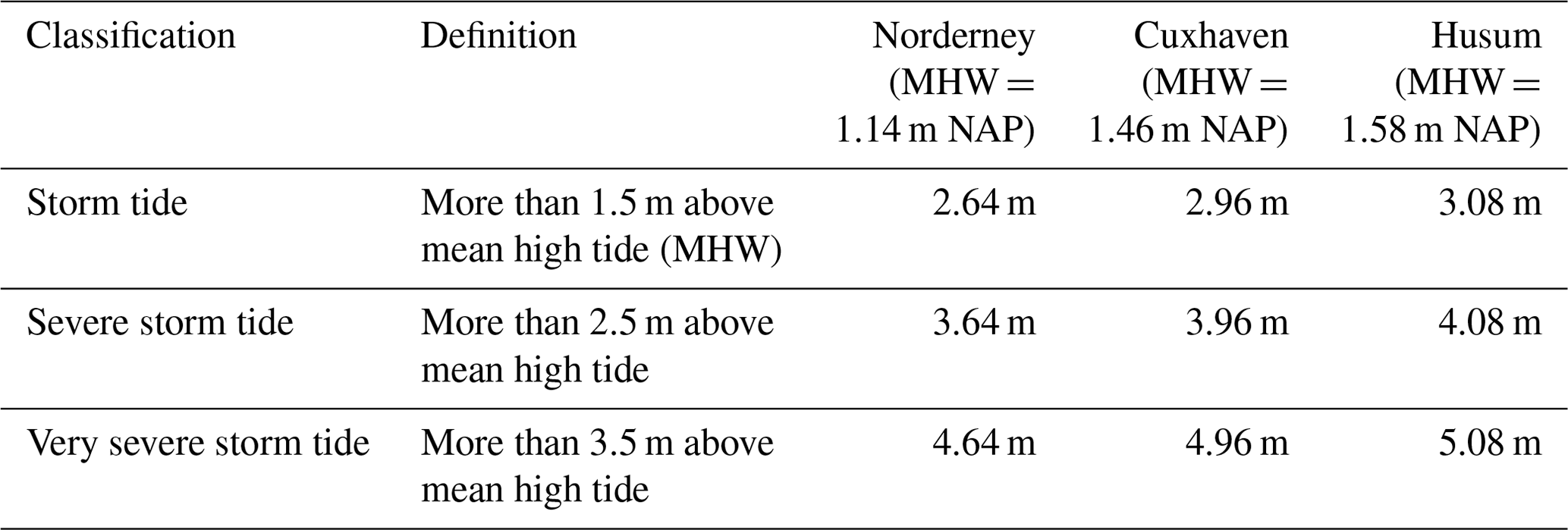
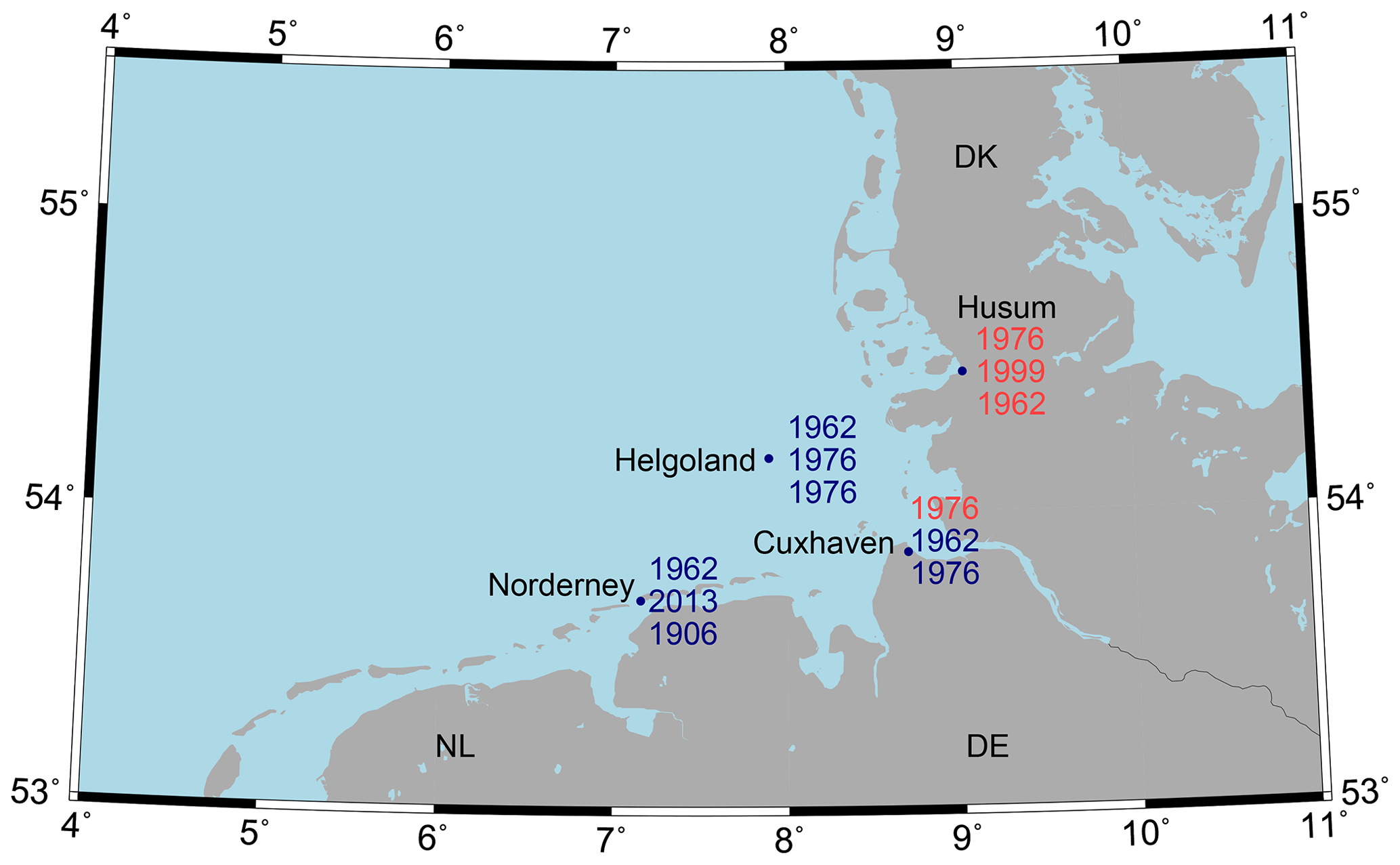
Figure 1 Three highest-water-level events observed since the beginning of regular observation at selected locations in the German Bight and their classification by the BSH (Table 1) as severe (blue) and very severe (red) storm tides.

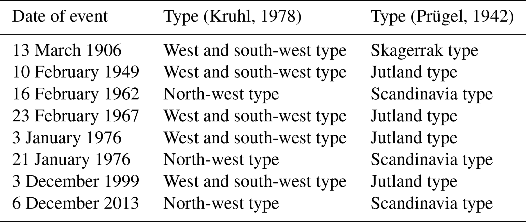
The risk potential of individual storms and storm tides changes along the German North Sea coasts depending on the specific storm tracks and associated wind directions and wind set-up. The tracks of storms which caused the most severe storm tides in one or another region of the German Bight coast are shown in Fig. 2; their description is complemented in Table 2. The tracks follow the minimum of the low-pressure area for each storm event with the sea-level pressure data derived from the ERA5 reanalysis starting from 1940. Several storm classification methods according to their tracks were proposed and discussed in the literature in the past decades (e.g. Kruhl, 1978; Gerber et al., 2016, or Prügel, 1942; Schelling, 1952; Petersen and Rhode, 1991). Summarising, the typical storms associated with the storm tide hazard in the German Bight can be separated into the north-west (or Scandinavia) type and the west and south-west (or Jutland) type. In particular, Prügel (1942) defined the types according to the latitude at which they crossed longitude 8^∘ E (see Fig. 2).

• Jutland type: 55–57^∘ N

• Skagerrak type: 57–60^∘ N

• Scandinavia type: 60–65^∘ N

The East Frisian coasts (southern German Bight) have higher water level risks during storms travelling more in the north of Europe. Such storms are labelled as Scandinavia type and are characterised by a long fetch over the North Sea area and high surge in the entire southern North Sea, e.g. storm tide in 1962 (Rodewald, 1962; Koopmann, 1962; Gönnert, 2003). The low-pressure system over Scandinavia and at the same time a high-pressure system in the Bay of Biscay generate high-pressure gradients and wind speed over the North Sea (Fig. A1, a–c).

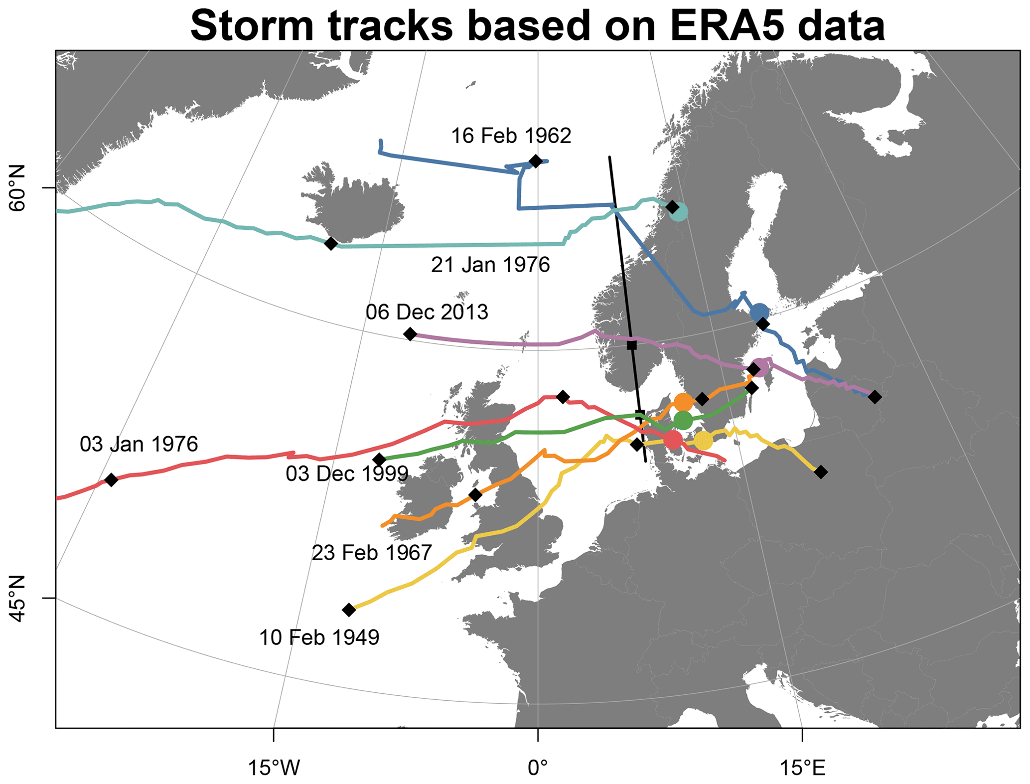
Figure 2 Storm tracks derived from ERA5 data. Black diamonds mark midnight on the track. The coloured circles mark a specific date when the observed water level in Cuxhaven was highest during this event. The black line depicts longitude 8^∘ E as the basis for the storm tide classification according to Prügel (1942). The squares separate the Jutland, Skagerrak and Scandinavia types. For additional information about mean sea-level pressure during the single events, see Fig. A1.

Table 2 In this study, a selection of severe storms and storm tides in the German Bight is investigated. See also Fig. 1.

Fast-moving storms with more southerly tracks, so-called Jutland type, are characterised by high wind speeds and steep wind surge in the eastern German Bight, e.g. the storm on 3 December 1999. The Elbe estuary is situated between the two regions, and storms of both types were able to cause some of the most extreme observed water levels there. The highest observed storm tide at Cuxhaven during the storm on 3 January 1976 was induced by a storm of the Jutland type (Fig. A1, d). The situation was exacerbated by the timing of the tide. Namely, the wind speed peak at the Elbe mouth co-occurred with low tide, thus preventing the tide propagated earlier upstream of the river from being released back to the North Sea, which led to an additional water level increase on top of the wind surge. The second highest storm tide in the Elbe estuary was caused by a storm of the Scandinavia type in 1962, which had a prominent impact on the entire German Bight.

Due to the partly stochastic nature of maximum storm surge and tidal high water coincidence (e.g. discussion in Horsburgh and Wilson, 2007), some extreme storm surges did not result in extreme storm tides at the coast. Still, such events are of interest because they present the atmospheric conditions which may lead to extreme water levels when coinciding with high tide. So, Fig. 2 shows additionally the tracks of two storm events which caused extreme surges during low tide and therefore did not lead to very high water levels. The first one, on 10 February 1949, is known for the highest observed surge in Husum and the second one, on 23 February 1967, for the highest observed wind speeds on Helgoland (Tomczak, 1950; Lamb, 2005).

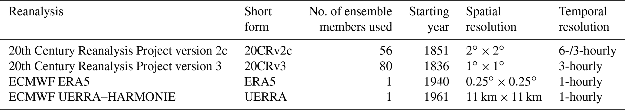
2.2 Atmospheric reanalysis products

The basis for this study is the century reanalysis data, in particular the products from the 20th Century Reanalysis Project (20CRv2c and 20CRv3) (Compo et al., 2011; Slivinski et al., 2019, 2021). This is an ensemble of global forecast model results with assimilated observations, e.g. pressure data from the International Surface Pressure Databank (ISPD). Observed pressure data have a long history and are robust concerning systematic measurement errors (Schmidt and von Storch, 1993; Alexandersson et al., 1998, 2000). Thus, the reanalysis dataset represents atmospheric conditions consistent with available observations but slightly varying due to internal variability, especially in the regions lacking measurement data. In total, 56 members for 20CRv2c and 80 members for 20CRv3 were used. Additionally, to the ensemble reanalyses, the results from the ECMWF (European Centre for Medium-Range Weather Forecasts) ERA5 and UERRA–HARMONIE, in the following UERRA, reanalysis were used (Hersbach et al., 2018; Ridal et al., 2018; UERRA, 2019). These data have higher spatial and temporal resolution, which may have an impact on the quality of the extreme water level simulations. As an additional refinement, the UERRA data were merged with OptempS data (Kristandt et al., 2014). In the OptempS project, high-resolution data in time and space were produced with a German forecast model to get more precise atmospheric conditions for the reconstruction of storm surges. A total of 40 events starting from 1960 were reanalysed in the project with ERA-40 (Uppala et al., 2005) and ERA-Interim (Dee et al., 2011) data used as initial conditions (Kristandt et al., 2014). The OptempS data are available approximately 3 d before and 2 d after the storm event. The main features of each dataset used are summarised in Table 3.

Table 3 Reanalysis data by 20CR and ECMWF used as forcing for the tide–surge model.

2.3 Tide–surge model

The water level simulations are done with the hydrodynamic tide–surge model TRIM-NP (Kapitza, 2008). TRIM is a tidal, residual and intertidal mudflat model that was originally developed by Casulli and Cattani (1994) and later nested and parallelised (NP) by Kapitza (2008). Pätsch et al. (2017) tested and validated the model; Gaslikova and Weisse (2013) used the model also to simulate multi-decadal hydrodynamic conditions including hindcast and climate change projections (e.g. Gaslikova et al., 2013). Callies et al. (2011) used the TRIM model data for drift simulations. Meyer et al. (2022) used this model to simulate the severe storm tides during the 1906 storm event.

All simulations are done in a barotropic mode within a three-level nested set-up with regular Cartesian grids, having spatial resolutions from 12.6 km for the north-east Atlantic and the North Sea (grid 1) down to 1.6 km for the German Bight (grid 4; Fig. 3). The tides are calculated separately by FES2004 (Lyard et al., 2006) and introduced at the lateral boundaries of the coarsest grid. All model simulations started at least 15 d before each storm event and used zonal and meridional 10 m height wind components and sea-level pressure fields from the corresponding reanalysis as atmospheric forcing.

To explore the potential for the storm tide amplification for selected events, the historical tide was interchanged with a spring tide to simulate the highest physically possible water level depending on the respective weather situation during the event.

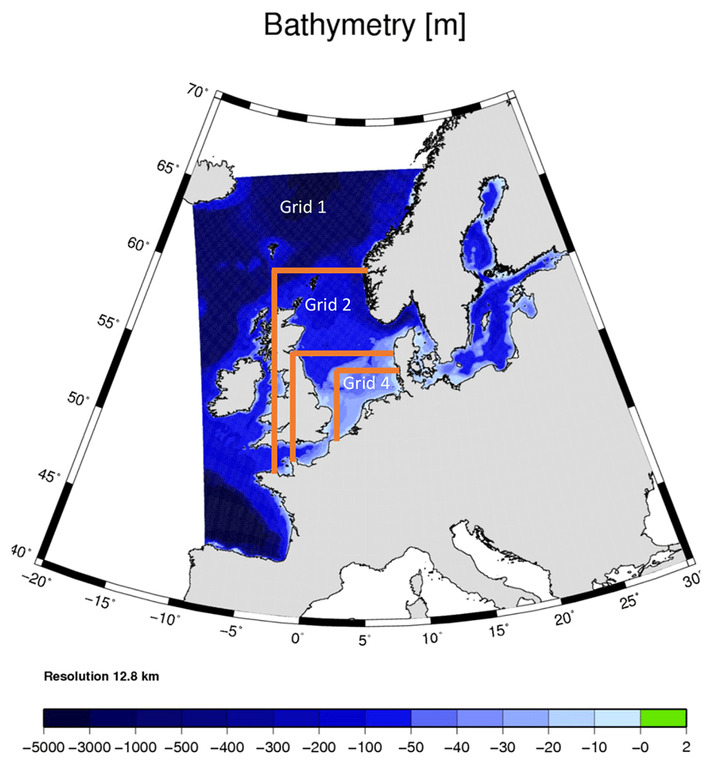
Figure 3 Trim model domain with grid 1 (12.8 km resolution), grid 2 (6.4 km), grid 3 (3.2 km) and grid 4 (1.6 km).

3 Results

3.1 Analysis of the storm tide event of 16 February 1962

On the example of one selected historical storm and a single location in the German Bight, we describe the temporal development of the storm and exemplarily the relations between different reanalyses and reanalysis members for both the storm tides and the underlying wind conditions. Figure 4 depicts the wind speeds near the island of Helgoland (Fig. 1) for 24 h before and after the storm peak for the 1962 storm extracted from all reanalyses used as representations of the marine atmospheric conditions in the German Bight. We do not use the observational wind data for comparison here because the wind measurements for Helgoland are somewhat impaired for certain wind conditions (Lindenberg et al., 2012) and it is not the topic of the present study to validate the reanalyses as that has been done extensively (Kristandt et al., 2014). During the 1962 storm, the wind speeds in the German Bight were not extremely high, but they exceeded 17.2 m s⁻¹ (8Bft, Gale) for a long period. The solid (coloured) lines represent ensemble members of 20CR reanalyses with the largest wind peak maximum. The grey lines show single members with a spread of about 7 m s⁻¹ for the peak wind speeds for 20CRv3 (light grey) and about 3 m s⁻¹ for 20CRv2c. The OptempS wind speeds, representing here the best-guess wind conditions, are on the upper boundary of both sets of reanalyses. UERRA wind speeds, being very similar to OptempS in the temporal average, exhibit 6-hourly peaks. This is a known feature originating from the UERRA-specific 6-hourly re-forecasting procedure and was discussed by, for example, Schimanke et al. (2020) and Andrée et al. (2021). The peak of the ERA5 wind speed lags behind the peaks of other products, and the wind speed is in general lower during the first half of the storm.

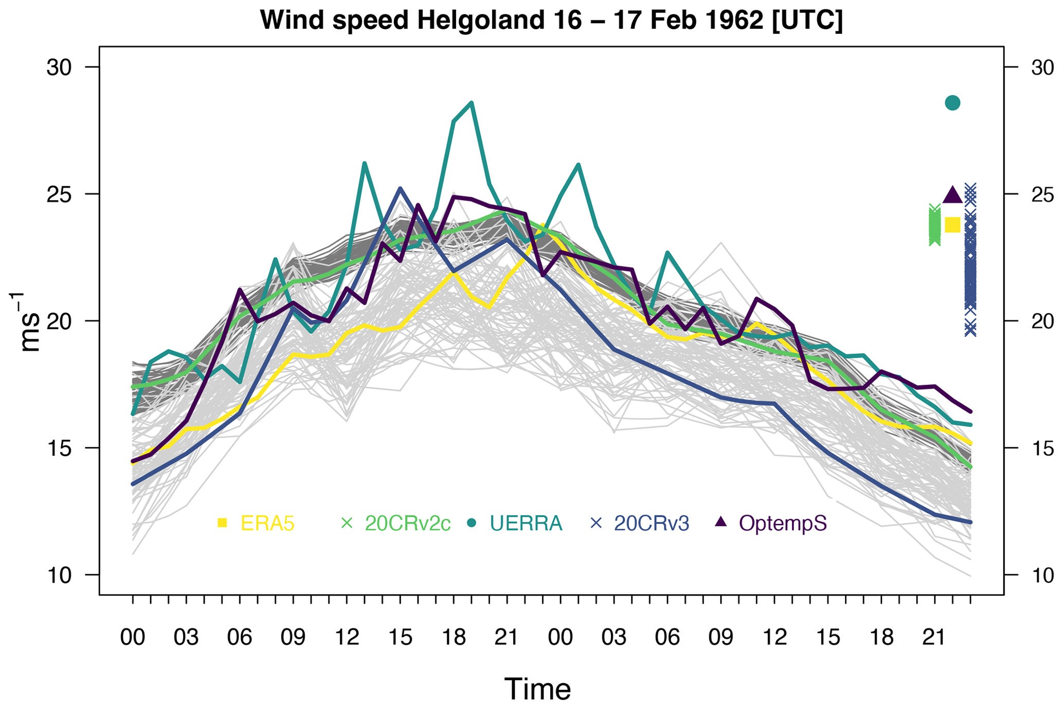
Figure 4 Wind speed near Helgoland for the event on 16/17 February 1962 from UERRA in dark cyan, OptempS in dark violet, ERA5 in yellow, and 20CRv2c (all ensemble members – dark grey; the member with the strongest wind – green) and 20CRv3 in light grey and blue for the highest member. On the right side, the highest peaks of the wind speed are shown for each reanalysis and each ensemble member.

The storm tides caused by the atmospheric conditions described are shown in Fig. 5 for Cuxhaven, located in the Elbe estuary (Fig.1). In addition to the reanalyses, the tide gauge measurements at the location are depicted for comparison. The storm tide event continues for three tidal cycles. For the peak high water the observations lie well within the range of the reanalysis ensemble. The range of the peak water levels from different reanalyses and reanalysis members is, however, rather high at about 1.5 m. Looking more into details, it can be inferred that results obtained with UERRA and OptempS forcings are very close to each other and slightly overestimate the observed peak high water. ERA5-driven storm tides underestimate the observed ones, which is consistent with the wind speed relation between ERA5 and UERRA–OptempS (Fig. 4). All 20CRv2c ensemble members overestimate observations and most of the other reanalyses, which agrees with the slightly higher 20CRv2c wind speeds during the first part of the storm (Fig. 4). Some of the ensemble members forced by the 20CRv3 are very close to the observations; however, the variability in the ensemble set is also large, following the variability in maximum wind speeds. We will follow the description of storm tide reanalyses for other storm events and locations using only the peak water levels from each realisation for comparison. For an explanation, see an example on the right side of Fig. 5.

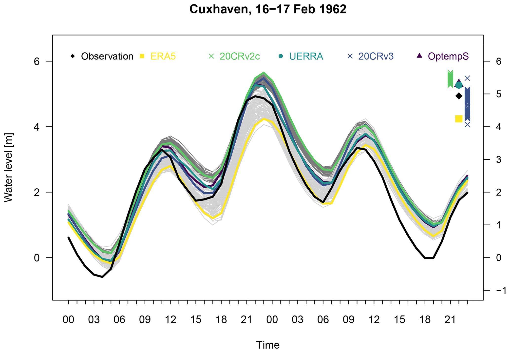
Figure 5 Observed and modelled water level for Cuxhaven for the event on 16/17 February 1962. Observations are in black, and simulated results are from model runs forced by various atmospheric reanalyses (see Fig. 4 for colour-coding).

3.2 Other storm tide events in the German Bight

To compare the effects of the eight investigated storms (see Table 2) on the water level at the different coastal strips of the German Bight, we selected the following stations (Fig. 1): (a) Norderney (southern German Bight), (b) Cuxhaven (Elbe estuary) and (c) Husum (eastern German Bight). The tidal conditions are different for the three selected locations as the tidal wave travels anticlockwise in the North Sea, interacts with the relief, and is formed by the combination of dissipation and reflection. In the German Bight, from east to west and from the open sea to the coast, there are differences of several decimetres in the tidal range (Siefert and Lassen, 1996). Therefore, the tidal range at Norderney (2.46 m) is smaller than at Cuxhaven (2.94 m) and Husum (3.50 m) (see also Table A1). This, of course, affects the absolute water level heights during extreme events but also the relative importance of the surge part for each storm tide.

Figure 6 shows storm tides from modelling results for the selected storm events at the three selected locations together with the corresponding observed maximum water levels. Additionally, for some events for which the potential for amplification was suspected, the results of additional experiments with tidal shift are shown. They represent the member of the 20CRv3 reconstruction which led to the highest storm tide and for which the water level simulation was repeated with the gradual temporal shift in spring tide instead of the historical tide. For the events with extreme surges that occurred during low tide, the observed low water is additionally depicted.

To discuss the results further, we subdivide the storm events according to the type of atmospheric situation they represent, as was described in Sect. 2.1. The multi-model ensemble exhibits similar behaviour within each type.

3.2.1 Scandinavia type

For the events of Scandinavia type – the storms of 1962, 21 January 1976 and 2013 with more northerly storm tracks (Fig. 2) – the modelling results show, in general, a reasonable agreement with observations (Fig. 6). From the 20CRv3 ensemble, there are at least several members which can reproduce historical hydrodynamic conditions for each event and at all three locations. The 20CRv2c ensemble displays less variability in peak water levels, although at least some members are still close to the observations, except for the 2013 event at Norderney and Cuxhaven (southern German Bight). This is consistent with a smaller variability in wind maxima for this ensemble compared to the next version: 20CRv3 (see Figs. 4 and 8). UERRA and OptempS reconstructions also provide realistic atmospheric conditions for the simulation of extreme storm tides, resulting in estimations of water level maxima lying within a 0.3 m (for 1962 and 21 January 1976 events) and 0.5 m (for 2013 event) range relative to observed values for all locations. Simulations driven by ERA5 atmospheric data generally underestimate the observed storm tides at all locations by several decimetres. This result could be anticipated from the wind conditions directly, with ERA5 winds typically having lower extreme wind speeds than, for example, UERRA or 20CRv3 during the selected storms (see, for example, Figs. 4 and 8). The Scandinavia type of storms often leads to large-scale storm surges, which affect the entire German Bight (e.g. Fig. 7a), leading to severe storm tides at all three selected locations and especially in the southern North Sea. In particular, during the storm of 1962, although water levels are slightly overestimated by UERRA and 20CRv2c reconstructions, at least four common members of the 20CRv3 ensemble could reproduce the observed extreme high water levels with the 10 cm accuracy at all three locations. This suggests the possibility of using the most-fitting ensemble members for the reconstruction of the hydrodynamic conditions during this event for the entire coastline of the German Bight, covering with certain confidence even the coastal regions where the observational data were not available.

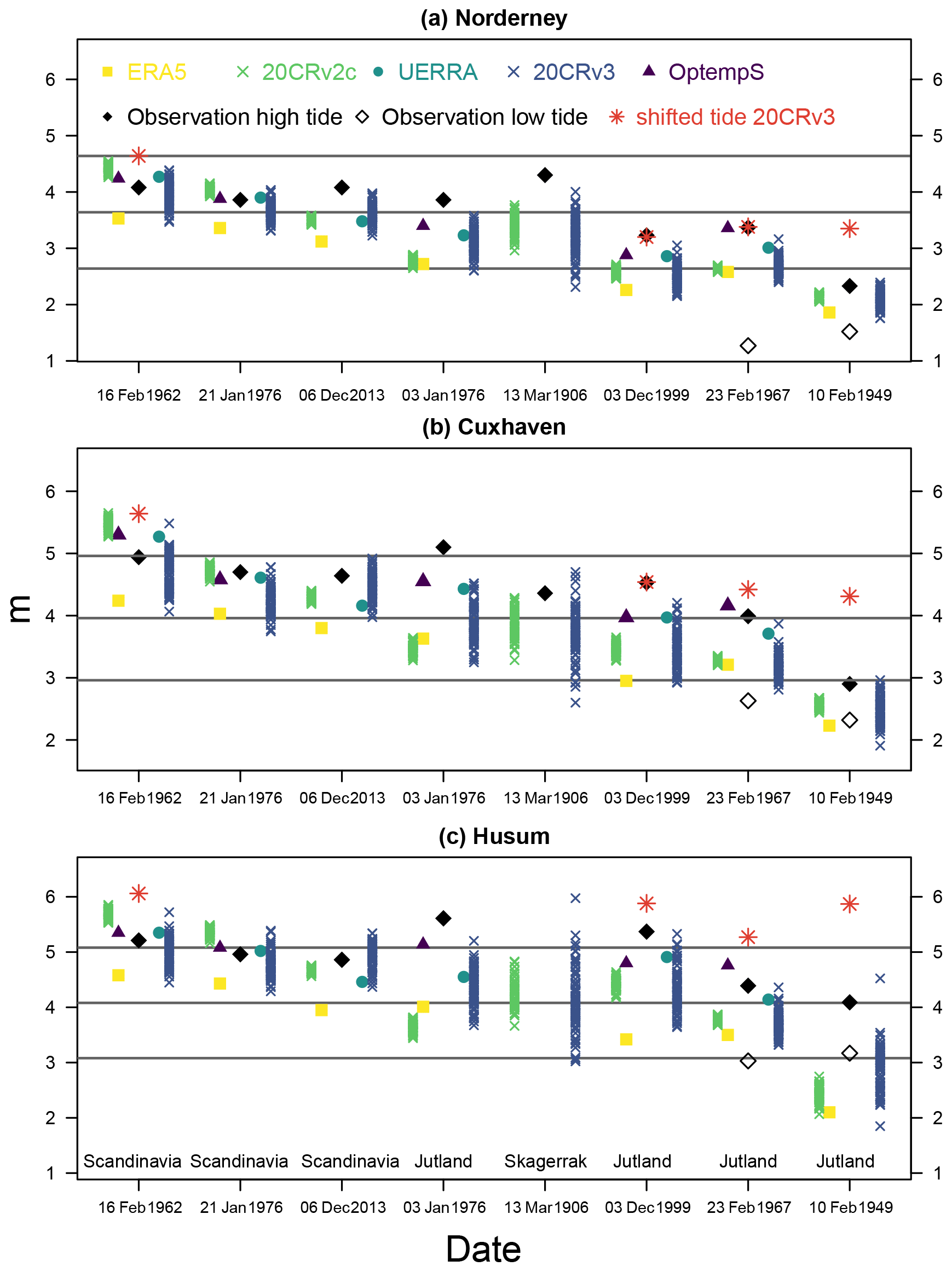
Figure 6 Maximum water levels in metres above normal Amsterdam level (Normaal Amsterdams Peil, NAP) for the three selected locations and the eight storm events. The different symbols and colours represent the different atmospheric forcings (see Table 2 and Fig. 4). The black diamonds stand for the observed water levels during high tide (filled) and low tide (unfilled). A red star marks the maximum water level from the tidal shift experiment for a selected member of the 20CRv3 reanalysis. The grey horizontal lines mark the level of very severe storm tide (top), severe storm tide (middle) and storm tide (bottom) for the respective locations (Table 1). The events are sorted according to the storm tracks crossing at 0^∘ longitude, and the types are defined crossing at 8^∘ longitude.

3.2.2 Skagerrak type

Following the classification of storm tracks, the next type is Skagerrak (Fig. A1) with storms moving along more southerly located trajectories. One of the representatives of such storms was the event of 13 May 1906, responsible for one of the highest observed water levels in the southern German Bight. The detailed analysis of this storm event, issues with the reconstruction of atmospheric conditions and the quality of the simulated storm tides can be found in Meyer et al. (2022). Here we show, for the sake of consistency, the ability of 20CR reanalysis to reproduce the storm consequences for Cuxhaven and Norderney. For Norderney, there were three reliable sources for observations available with the maximum water levels ranging from 3.84 to 4.30 m (Meyer et al., 2022). Depending on which observation source is considered more trustworthy, either the peak water level is slightly underestimated by all results of hydrodynamic modelling or selected ensemble members are able to reproduce the peak water level. For Cuxhaven, several members of hydrodynamic reanalysis show peak water levels close to the observed conditions.

3.2.3 Jutland type

The representatives of the Jutland type of storms – 3 January 1976 and 3 December 1999 – are relatively fast storms moving through the North Sea almost from west to east (Fig. 2). With the cold front passing through the German Bight, they are characterised as being shorter in duration but more intensive in wind speed extremes from south-westerly–westerly directions and rapidly changing directions shortly before the storm peak in the German Bight (Fig. A2). This makes it more difficult for atmospheric reconstructions to capture and reproduce the particularities of the storm, which is reflected also in the results for peak water levels. All considered reconstructions underestimate the peak water levels for both storms and all locations (Fig. 6; see also Table A3 for quantitative statistics). Although some members of the 20CRv3 reconstruction led to water levels close to the observed ones, the previous version 20CRv2c and ERA5 have difficulties in reproducing the exact historical storm conditions. It is assumed that, particularly for the storm on 3 January 1976, the atmospheric reconstructions may be lacking some short-term or small-scale meteorological phenomena crucial for the extreme storm surge formation.

3.2.4 Differences in water level and surge between Scandinavia and Jutland types

To illustrate the effects of storm tracks on the spatial distribution of water levels in the North Sea, Fig. 7 summarises the results for two storm events that exemplify the Scandinavia (16/17 February 1962; Fig. 7a–c) and the Jutland types (3 January 1976; Fig. 7d–f) of storm tracks. Both events caused the two highest observed water levels in Cuxhaven during the last century.

The panels show water level (Fig. 7a, d), tide (Fig. 7b, e) and surge as non-tidal residual (Fig. 7c, f) at the time of peak water level in Cuxhaven during the corresponding event as modelled using the merged atmospheric UERRA–OptempS forcing. The tidal component is estimated by model simulations without atmospheric forcing. Non-tidal residuals comprise (Fig. 7c, f) wind surge and external surge but also consider the inverse barometer effect and non-linear tide–surge interactions. In both situations, storm peaks approximately co-occurred with high tide in the German Bight (Fig. 7b, e). For the event in 1962, the whole German Bight was affected by very high water and surge levels (Fig, 7a, c), whereas, during the event in 1976, only the east coast of the German Bight and the Elbe estuary experienced a very severe storm tide (Fig. 7d, f). Storm tracks of the Jutland type are moving much faster over the North Sea and have a shorter impact on the water level than the storms with northerly tracks. During the storm in 1962, additionally, a large contribution of external surge (Koopmann, 1962) raised the high surge in the entire southern North Sea. This phenomenon is mainly associated with the influence of low-pressure systems in the north-east Atlantic via the inverse barometer effect, then enhancement at the continental shelf and finally propagation into the North Sea (e.g. Böhme et al., 2023). Thus, the ability of atmospheric reconstructions to represent the intensity, location and speed of the low-pressure system in the north-east Atlantic also contributes to a more realistic representation of the storm tides in the German Bight.

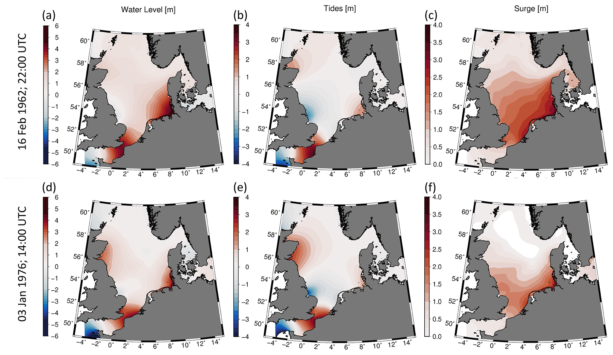
Figure 7 Exemplary spatial distributions of water levels (a, d), tides (b, e) and surges (c, f) at the moment of maximum water level in Cuxhaven for the Scandinavia-type storm (represented by the event of 16 February 1962, upper row) and the Jutland-type storm (represented by the event 3 January 1976, lower row) modelled with the wind forcing by OptempS.

3.3 Variability and uncertainties due to atmospheric conditions

Taking advantage of the ensemble reconstructions, we look now at the effect of internal variability for each investigated storm event (Table 2). As a representative of atmospheric conditions in the German Bight, the wind speeds near Helgoland were selected. Figure 8 shows the maximum wind speeds for each considered storm obtained from each reanalysis or reanalysis member. There are several features of inter-reanalysis relations specific to different storms. For example, OptempS and UERRA wind maxima, showing always one of highest wind speeds among all reanalyses, are sometimes close to each other (e.g. for 3 January 1976 or 3 December 1999 storms) and for other events are different and exceeding all other reanalyses (e.g. 1962, 1967, 21 January 1976 storms). This can partly be attributed to somewhat artificial 6-hourly wind speed peaks in UERRA discussed for the 1962 storm example. These do not have a strong effect on the storm tide extremes, as can be seen for the 1962 and 21 January 1976 example storms in Figs. 5 and 6. Another distinction between the storms is the magnitude of 20CRv2c extremes relative to 20CRv3 extremes. Namely, they are sometimes at the upper range (e.g. for 1962), at the low range (e.g. 1967) or somewhere in between as for all other storms. These relations are not always transferable to the storm tide extremes, e.g. for the storm of 3 January 1976.

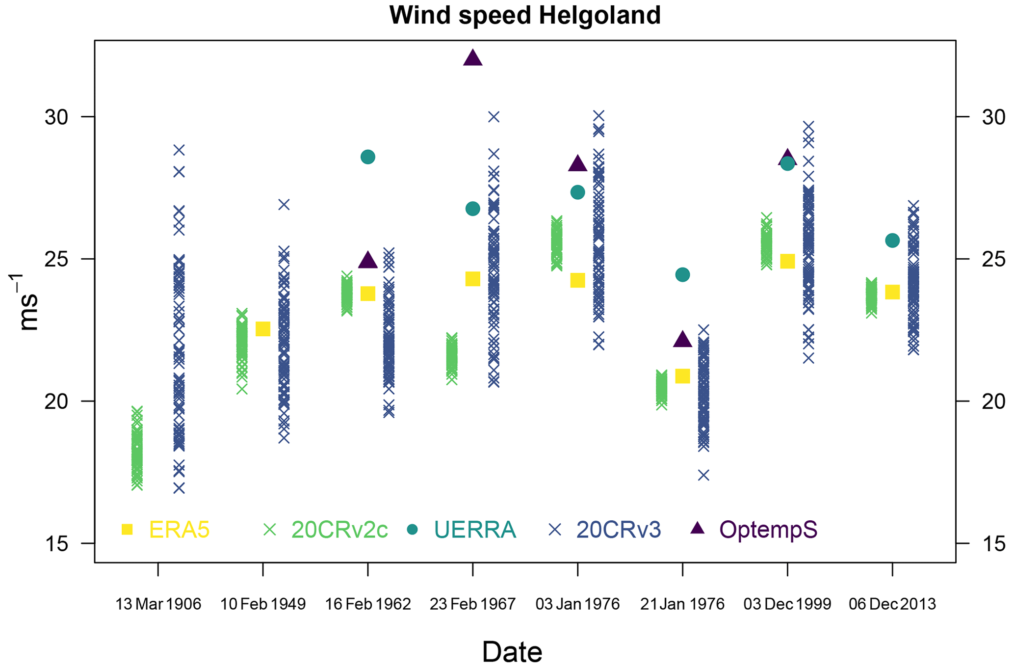
Figure 8 Maximum wind speed simulated by the reanalyses for the location of Helgoland during each event. See also Table A2 and Fig. A2.

There are also some features which are common for all considered storm events. For example, the wind speed maxima from ERA5 reanalysis are generally lower than those from UERRA–OptempS and are within the range of the 20CRv3 ensemble. It is noticeable that the wind speeds from ERA5 are not higher than 25 m s⁻¹ during these severe storm events. Haakenstad et al. (2021) and Dullaart et al. (2020) show that ERA5 underestimates very high wind speed compared to the observations. This is also reflected in the related storm tide extremes (Fig. 6), where extreme water levels forced by ERA5 lie at the lower range of other reanalyses and typically underestimate observations.

When we look at the spread of the wind maxima for different storms, the earlier storms, in particular 1906, show larger variability than more recent storms. This can be attributed to a smaller number of available observations for that period and thus less assimilated data, which leads to more degrees of freedom for the atmospheric circulation. In the year 1949, a large amount of data from the relevant regions had already been assimilated into the model for the Northern Hemisphere. Only surface pressure and wind data were used in the 20CR reanalysis, skipping the substantial increase in data available from satellites starting from 1980.

This may increase the uncertainty of the 20CR reanalysis for the recent decades with respect to other datasets; however, it ensures the consistency of the data quality throughout the whole reanalysis period. This, in turn, enables us to notice the following differences in variability between the considered storms: it can be inferred (e.g. Fig. 8 and Table A2) that both 20CR ensembles demonstrate a larger uncertainty range of the maximum wind speed for the storms of the Jutland type and notably smaller uncertainty for the Scandinavia type. As has been described earlier, during the Jutland-type storms the low-pressure area travels directly through the North Sea (e.g. Fig. A1), and the exact position and travel velocity of the low strongly influence the local wind speed and direction over the North Sea. Thus, the minor variations in the storm track or timing due to natural variability led to relatively large changes in the local wind speed maxima in the German Bight. Whereas for the Scandinavia-type storms, with low-pressure areas travelling mostly beyond the North Sea, the wind is not that sensitive to the minor variations in the position and travel velocity of the low. It is also easier for other reanalyses with only one realisation to be more realistic in wind representation for the Scandinavia type, which makes it easier to reconstruct the storm tides realistically for these types of storms and it takes more effort to make it for the Jutland type, as is the case for the 3 January 1976 storm.

Another characteristic common to all storm events is a significantly smaller variability in the 20CRv2c ensemble with respect to 20CRv3 (Fig. 8 and Table A2). Whereas 20CRv2c wind speed maxima from different members are spread by 1.1 to 2.6 m s⁻¹ for a single location depending on the storm event, the 20CRv3 members are spread by 5.1 up to 11.9 m s⁻¹. The difference between 20CRv2c and 20CRv3 originates mainly in the different assimilation schemes and improved forecast systems by the National Centers for Environmental Prediction (NCEP) with higher resolution in both time and space (Slivinsky et al., 2019). The different uncertainty rates are also noticeable in the storm tide ensembles (Fig. 6, Table A3). For 20CRv2c, the peak storm tides spread between 0.15 and 1 m for various storm events with a median of 0.34 m. For 20CRv3, the spread increases to 0.95–2.1 m with a median of 1.16 m. These uncertainties are associated with the natural variability only, e.g. the slightly shifted location, timing or strength of atmospheric low-pressure system and consequent variability in high-wind-speed directions, duration and magnitude. Being physically consistent with the historical large-scale atmospheric conditions, these atmospheric realisations represent possible realistic developments of certain historic storms and thus realistic storm tides. It should be noted that some ensemble members of both 20CR reanalyses led to higher water levels than observed ones, hinting at potential amplification of storm tides within the historical settings. This should be considered, for example, for coastal protection design, which rests upon historic water level extremes, among other criteria. Another point worth mentioning is that the ensemble mean values of maximum water levels underestimate the observed values almost for all events and both ensembles, with the exception of 1962 and 21 January 1976 storms simulated with 20CRv2c (Table A3). Whereas the selected ensemble members can reproduce or come close to the observed extreme water levels, especially for the Scandinavia-type storms, the ensemble mean underestimation reaches up to 1.6 m. Specifically for Jutland-type events, the use of ensemble mean values for the representation of water level extremes is not recommended.

3.4 Amplification of storm tides by shifting tides

The storm events in 1949 and 1967, mentioned in Table 2 but not discussed so far, exhibited extreme atmospheric conditions but did not lead to extreme water levels at the coast. The event in 1967 was distinguished by exceptionally high wind speeds in the German Bight, and the event in 1949 led to the highest recorded storm surge near Husum (Figs. 6 and 8). During both events, the peak water levels were not noticeably high. The observed low waters at Husum, however, were the highest from the beginning of the record, indicating the presence of exceptionally high storm surges. Both events are reasonably represented, although they are slightly underestimated by at least some members of the water level reconstructions.

These two storm events represent examples of events which possibly could generate more severe peak water levels in the case of a more unfortunate temporal coincidence of the storm peaks and high tide, especially spring high tide. To analyse the potential of these historical storm tides for amplification, physically consistent with the real conditions, additional numerical experiments were done. The member of the 20CRv3 ensemble which produced the highest storm tides during each event was selected to investigate whether these storm events could have caused much higher water levels at the coast under different tidal conditions. In the numerical experiments a spring tide and temporal shift in the tide were used together with the historical atmospheric conditions. It can be concluded, based on BSH categorisation for Norderney and Cuxhaven, that such storms would not result in very severe storm tides in any case, though the 1949 storm had more potential for an increase (about 1 m for Norderney and about 1.35 m for Cuxhaven). For Husum, if the event of 1949 had happened under more unfavourable conditions, it would have led to very severe storm tides comparable to the historically observed maximum water level (Fig. 6). Such considerable amplification can be partly explained by the larger tidal range near Husum and the funnel-shaped coastline, which exacerbate the changes by a switch from low tide to high spring tide. Additionally, being the Jutland type of storms, the 1949 and 1967 events caused a more pronounced surge at the eastern coast of the German Bight, affecting Husum at most of the three selected locations.

The possibility of higher water levels during different tidal conditions was also investigated for the events in 1962 and 1999. The ensemble members with the highest water level for 1962 and 1999 produced by 20CRv3 were shifted to a spring tide. In 1962, the simulated water level was already higher than the observed ones. This is the case for all locations and presents the highest water level for all events: 4.64 m for Norderney, 5.64 m for Cuxhaven and 6.06 m for Husum. The water levels for the 1999 event were underestimated compared to the observed ones, but with the amplification of the tides, the water levels become higher, particularly in Husum.

4 Conclusions

We investigated some of the most prominent storm tides observed in the German Bight during the last 120 years. The water levels associated with the storms were simulated with a tide–surge model using atmospheric forcing from different reanalysis products (20CR, ERA5 and UERRA). The resulting extreme storm tides were compared with observations for three locations at different coastal strips of the German Bight. The comparison of storm tide extremes with measurements gives a hint of the quality of the wind and pressure data and their capability to represent the atmospheric conditions during extreme storm events.

In our investigation, we could show that the historical severe storm tides could be simulated realistically with individual members of 20CRv3, UERRA–HARMONIE and the merged UERRA–HARMONIE–OptempS reanalysis. Only the 3 January 1976 event could not be simulated satisfactorily using any of the considered reanalysis products, and the 1999 event was difficult to represent for the southern German Bight. The ERA5 data did not provide higher wind speed than 25 m s⁻¹ close to the Helgoland location, and all water level results are lower than the observed ones at the coast. Some differences between observed and modelled water levels were expected due to a range of factors not related to the atmospheric drivers. For example, the considered historical storm events occurred within the last 120 years, during which there were significant changes in bathymetry, especially in the shallower areas and estuaries. Changes in the coastline due to erosion, consolidation and extensive protection constructions also took place. Additionally, the mean sea-level rise is manifested in the region with changes of about 25 cm during the period. All these changes were not accounted for in the present study. Additionally, there is a limitation due to the hydrodynamic model spatial resolution of 1.6 km and the ambiguity of some observational data, especially for older storms (e.g. 1906).

The maximum wind speeds during the storms showed more variability for the 20CRv3 ensemble than for 20CRv2c, and the range encompassed the maximum winds from most of the other reconstructions. It translates also into the variability in storm tide peaks, leading to the differences from 0.95 to 2.1 m between the 20CRv3 reconstruction members depending on the storm event. This uncertainty, representing the internal variability in the atmospheric system, indicates the realistic range of extreme storm tides associated with certain atmospheric situations. We have also considered an amplification mechanism due to a combination of atmospheric and non-atmospheric conditions; in particular, we have shifted the tidal high water to coincide with the wind speed peak to get information on what is physically possible for the worst high water level at the coast. In these experiments, the extreme water levels would increase by a few decimetres. For the storm events of 1949 and 1967 with shifted tides, the peak water levels would not be higher than the ones already observed in Norderney and Cuxhaven. For Husum, this experiment produced one of the highest observed or simulated water levels. This can be attributed mainly to the funnel-shaped coastline and larger tidal range near the location but also storm surge distribution, which for these particular storms affected more the eastern than the southern parts of the German Bight. Shifting the tides to spring tide for the 1962 event resulted in the highest simulated water levels for all three locations. Generally, the shift in the tides shows a higher effect for the eastern German Bight than for the southern German Bight for the considered storms (Fig. 6).

Furthermore, in our investigations we have distinguished between the Scandinavia, Skagerrak and Jutland types of storm tracks over the North Sea and investigated their impact on the water levels on the German Bight coast. The northerly storm tracks cause a high surge over the entire southern North Sea. The southern storm tracks cause high surges on the eastern side of the German Bight (Fig. 7). Generally, the water level in the German Bight can be simulated using reanalysis data, but the accuracy of reproducing the observed extreme water levels depends partly on the type of storm track. The simulated water levels in the German Bight coast are more uncertain and mostly underestimated compared to the observations when the storm is categorised as Jutland type. One reason may be the incomplete reconstruction of the fast-running low over the southern North Sea (Fig. 2) in the atmospheric forcing data.

In summary, the various atmospheric reanalysis products are useful forcing data for investigating historical storm tides and their effects on the coasts. The study of historical storm tides, on the other hand, may be considered for risk management in the case of coastal protection, which rests upon historical water level extremes among others.

However, there are still historical events that would benefit from further improvement in the atmospheric data with new digitised historical pressure data, e.g. the severe storm in the Baltic Sea region in November 1872 (Feuchter et al., 2013; Rosenhagen and Bork, 2009). Hawkins et al. (2023), for example, have shown that with new digitised historical pressure data and an improved data assimilation process, the reanalysis of the severe windstorm over England and Wales in February 1903 could be significantly improved. Also, the simulations of the severe storm tides with a low-pressure area moving centrally over the North Sea, like the 3 January 1976 and 3 December 1999 events, need further improvements. These examples show that further investigations and modelling efforts for severe windstorms and the resulting storm tides could be beneficial. This would concern both the forecasting capability and thus the immediate risk awareness, as well as the reconstruction potential, and thus the long-term planning of coastal protection and management.

Appendix A

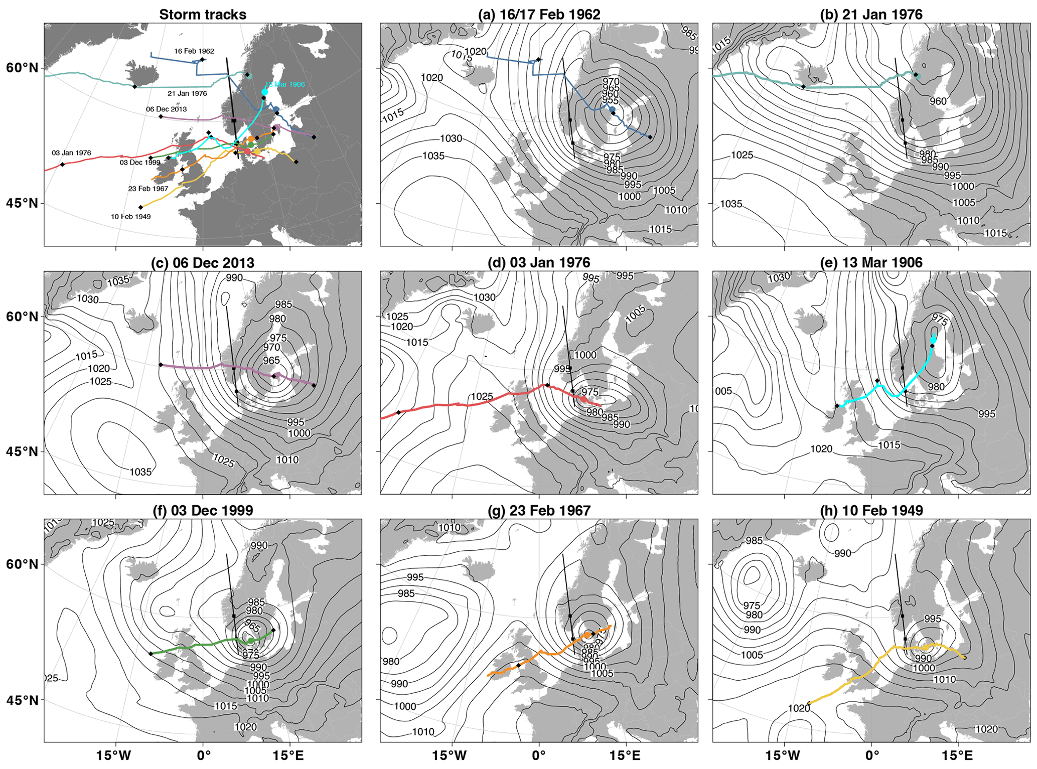
Figure A1 Storm tracks and mean sea-level pressure at the high peak of the storm are shown for the Scandinavia type (a–c), Skagerrak type (e) and the Jutland type (d, f–h). The events are sorted according to the latitude of the storm tracks at longitude 0^∘. All tracks and mean sea-level pressure data are from ERA 5, only panel (e) is calculated from 20CRv3. The tracks are divided at 8^∘ E into categories for the different types according to Prügel (1942) (black line).

Table A1 Information about the locations of the tide gauges and their range over 2004–2013 (10-year mean; Deutsches Gewässerkundliches Jahrbuch, 2014).

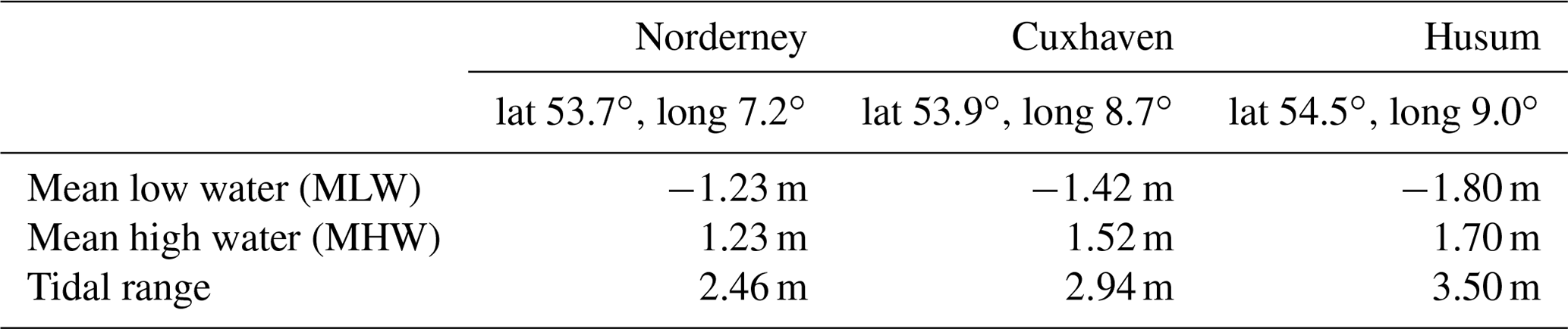
Table A2 Statistics of maximum wind speed (m s⁻¹) of the ensembles during the severe storm event for the 20CRv2c and 20CRv3 products and OptempS for the location of Helgoland.

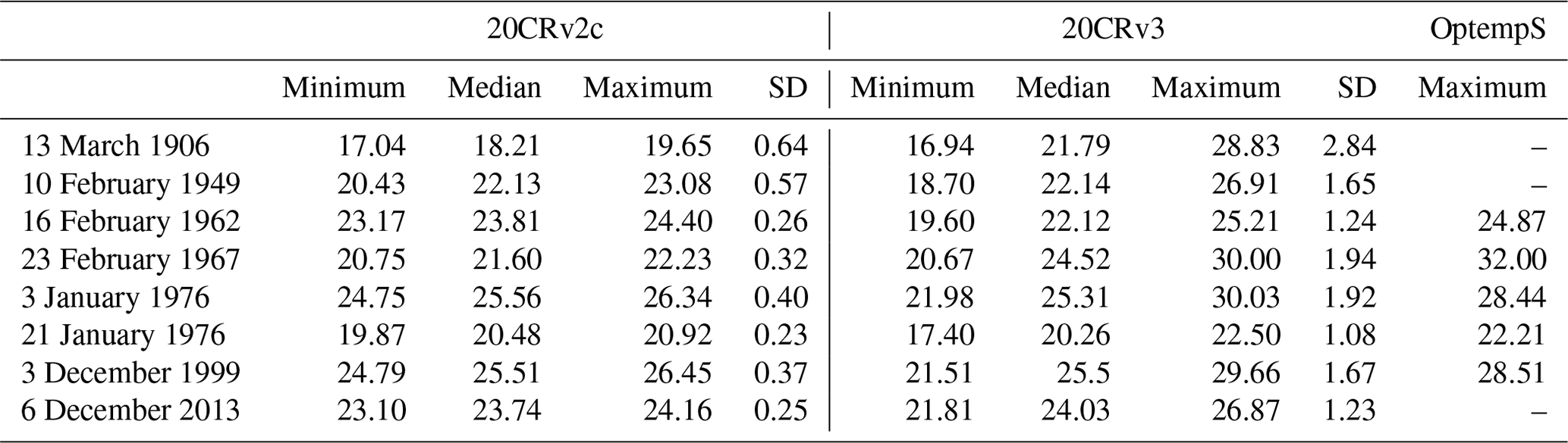
Table A3 Statistics of modelled water levels by 20CRv2c and by 20CRv3 and observations (Obs.) for the location Cuxhaven.

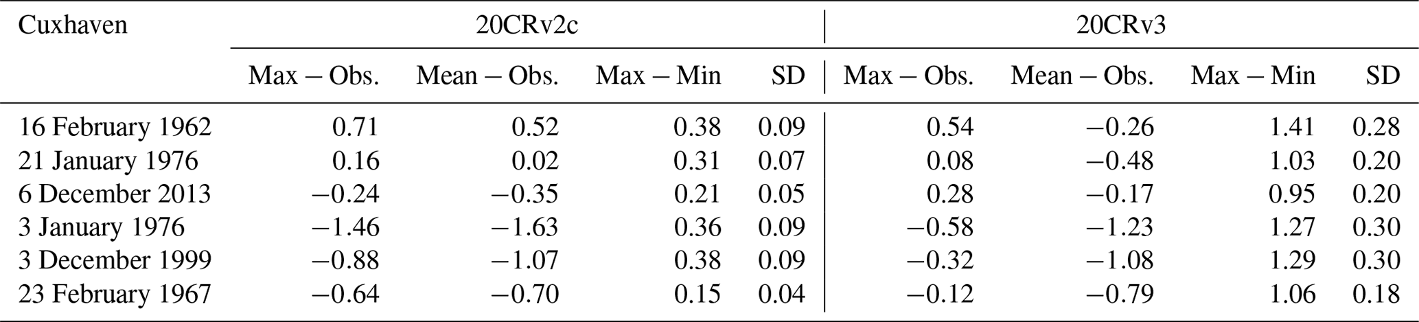
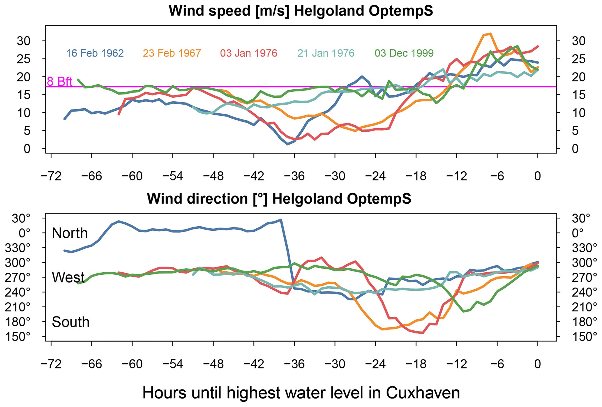
Figure A2 Wind speed and direction for the location of Helgoland in hours before the highest water level in Cuxhaven. The colours indicate the specific event. The light and dark blue colours indicate storms, which are categorised as Scandinavia type, and the others are the Jutland type (orange, red, green).