A multivariate statistical framework for mixed storm types in compound flood analysis

In coastal regions, compound flooding can arise from a combination of different drivers, such as storm surges, high tides, excess river discharge, and rainfall. Compound flood potential is often assessed by quantifying the dependence and joint probabilities of flood drivers using multivariate models. However, most of these studies assume that all extreme events originate from a single population. This assumption may not be valid for regions where flooding can arise from different generation processes, e.g., tropical cyclones (TCs) and extratropical cyclones (ETCs). Here we present a flexible copula-based statistical framework to assess compound flood potential from multiple flood drivers while explicitly accounting for different storm types. The proposed framework is applied to Gloucester City, New Jersey, and St. Petersburg, Florida, as case studies. Our results highlight the importance of characterizing the contributions from TCs and non-TCs separately to avoid potential underestimation of the compound flood potential. In both study regions, TCs modulate the tails of the joint distributions (events with higher return periods), while non-TC events have a strong effect on events with low to moderate joint return periods. We show that relying solely on TCs may be inadequate when estimating compound flood risk in coastal catchments that are also exposed to other storm types. We also assess the impact of non-classified storms that are not linked to either TCs or ETCs in the region (such as locally generated convective rainfall events and remotely forced storm surges). The presented study utilizes historical data and analyzes two populations, but the framework is flexible and can be extended to account for additional storm types (e.g., storms with certain tracks or other characteristics) or can be used with model output data including hindcasts or future projections.

1 Introduction

Growing attention in scientific research has been directed towards compound extreme events resulting from various hydrometeorological drivers, as their impacts are often more severe than those caused by univariate events (e.g., Wahl et al., 2015). Recent studies have highlighted the threat of compound flooding in low-lying coastal and riverine regions that is generally driven by the combination of precipitation, wind-generated storm surge, and streamflow (Hendry et al., 2019; Nasr et al., 2023; Wahl et al., 2015; Ward et al., 2018). Given the potentially devastating consequences of such events, the ability to quantify their likelihoods is crucial for flood risk assessments, infrastructure design, urban planning, (re-)insurance markets, and emergency response, among others.

There are two general methods that have been used in the literature to study compound flooding. The first one focuses on quantifying the compound flood potential by analyzing the dependencies and joint probabilities among compound flood drivers (Couasnon et al., 2020; Hendry et al., 2019; Moftakhari et al., 2017; Ward et al., 2018; Zheng et al., 2013). The second one focuses on quantifying compound flood hazard by employing physics-based models to obtain flood depths and spatial extents of historic flood events (Kumbier et al., 2018; Silva-Araya et al., 2018; Torres et al., 2015; Nederhoff et al., 2024) or for large sets of synthetic events, where flood models are forced with boundary conditions of multiple flood sources (Bass and Bedient, 2018; Gori et al., 2020; Gori and Lin, 2022). Those boundary conditions can come from physics-based models (e.g., Gori et al., 2020) or statistical models (e.g., Jane et al., 2020). In either case, due to the requirement of numerous numerical model simulations, this approach is associated with large computational costs.

Calculating the probabilities of compound flood events is crucial and can be done either by applying extreme value analysis to flood depth information (Bass and Bedient, 2018; Gori et al., 2020; Gori and Lin, 2022; Nederhoff et al., 2024) or by using multivariate models to quantify joint probabilities of the flooding drivers (e.g., Chen et al., 2012; Couasnon et al., 2020; Jane et al., 2020; Lian et al., 2013; Moftakhari et al., 2017; Sebastian et al., 2017; Zheng et al., 2014). For the latter, statistical techniques that have been used include Bayesian networks (Sebastian et al., 2017), bivariate threshold-excess models (Zheng et al., 2014), a bivariate point process method (Zheng et al., 2014), and copulas (Chen et al., 2012; Couasnon et al., 2020; Jane et al., 2020; Lian et al., 2013; Moftakhari et al., 2017; Xu et al., 2018). Copulas have been extensively used to characterize the joint distribution of flood drivers due to their ability to model the dependence structure independently of the marginal distributions. However, most of these studies assume that all extreme events originate from a single population, which refers to a set of events or observations that share common characteristics and are generated by similar underlying processes. This assumption may not be valid for regions where flood drivers can arise from different generation processes and mechanisms (e.g., Barth et al., 2019; Smith et al., 2011; Kim et al., 2023). For example, both tropical cyclones (TCs) and extratropical cyclones (ETCs) can create extreme precipitation and extreme storm surges in the same coastal region, leading to compound flooding. Lai et al. (2021) estimated that TCs and ETCs are the major triggers of compound flooding. They found that more than 80 % of compound flood potential in East Asia and more than 50 % in the Gulf of Mexico is associated with TCs, while ETCs contribute the most in Europe. TCs generally create more intense winds and rainfall (RF) compared to ETCs, while ETCs generally have greater spatial extents and can create RF over longer durations (e.g., Orton et al., 2016; Sinclair et al., 2020). Therefore, the flood drivers generated by these two storm types have different characteristics that may not be well captured by fitting them into a single probability distribution. Furthermore, Kim et al. (2023) highlighted that extreme events generated by TCs have a stronger correlation between RF and storm surge compared to the rest of the events they studied in the Dickinson Bayou watershed in Texas. This implies that the above-mentioned assumption of data coming from a single population could lead to a mischaracterization of the compound flood potential and/or compound flood hazard (from hereon we use compound flood potential since the focus is on the statistical framework, but it can also be used as a starting point to assess compound flood hazard when coupled with a flood model).

Nederhoff et al. (2024) addressed this aspect by employing a compound flood model for the coast of the US, from Virginia to Florida. They separately simulated the total water levels induced by TCs and ETCs to assess their relative contributions and followed the approach outlined by Dullaart et al. (2021) to calculate the combined return water levels. Additionally, a few studies addressed this aspect from the standpoint of coastal sea levels (i.e., univariate). For example, Orton et al. (2016) and Dullaart et al. (2021) quantified storm tide return periods by separately analyzing TCs and ETCs. In contrast, Lai et al. (2021) utilized copulas to model joint probabilities of flood drivers (RF and storm surge) for TCs and ETCs separately. Their study provides insights into the relative contribution of each storm type for joint probabilities but does not quantify the combined hazard. While Lai et al. (2021) and Kim et al. (2023) provided a starting point toward separating compound flood drivers by storm types, a comprehensive multivariate statistical framework for assessing compound flood potential from mixed populations does not currently exist.

An additional key aspect is analyzing compound flooding for future climate conditions where it will likely be amplified due to global warming (Bates et al., 2021). This is typically achieved by incorporating future sea level rise (SLR) projections and future storm climatologies derived from general circulation models (Bates et al., 2021; Bermúdez et al., 2021; Bevacqua et al., 2019; Gori and Lin, 2022; Khanam et al., 2021). However, the low resolution of available general circulation models presents a challenge in capturing locally generated RF events, especially those related to convection (Imada and Kawase, 2021). Heavy precipitation can be caused by convection without being influenced by any cyclonic activity in the near atmosphere (Pfahl and Wernli, 2012). When combined even with small storm surges or just high astronomical tides, such events can lead to compound flooding where gravity-fed drainage is impeded by higher-than-normal coastal water levels. Therefore, it is important to understand the role of these types of events in driving compound flood potential, especially when including future projections from general circulation models that are not capable of capturing them.

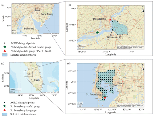
Figure 1 Study site locations; selected catchment boundaries; and locations of the rainfall gauges, tide gauges, and grid points of the Analysis of Record for Calibration (AORC) data for Gloucester City (a, b) and St. Petersburg (c, d).

Prior studies employing synthetic TCs for compound flood analyses have typically selected events that either crossed a specific search radius (e.g., Gori et al., 2020) or were generated in the study region (e.g., Bass and Bedient, 2018). However, cyclonic activity from distant systems can also generate moderate storm surges that propagate into the study region and, when combined with high tides and locally generated RF, can contribute to compound flooding. Hence, it is important to evaluate the potential mischaracterization of compound flood potential by neglecting such distant cyclonic events. Both of these questions regarding the role of local RF and remotely forced storm surge events have not been addressed in the literature.

This paper fills the above-mentioned gaps by introducing a copula-based statistical framework to estimate the compound flood potential at the catchment scale while accounting for mixed storm populations. We estimate the combined joint exceedance probabilities for different storm types and analyze the contribution of TCs, ETCs, and non-classified events (i.e., local RF and remotely forced storm surges). The framework is applied to Gloucester City, New Jersey, and St. Petersburg, Florida, as case studies.

2 Case study site and data

2.1 Study sites

Gloucester City is located in Camden County, New Jersey, along the Delaware River (Fig. 1a) where it accommodates approximately 11 400 residents (City of Gloucester, 2024, New Jersey). The city was affected by several major flood events in the recent past generated by hurricanes and severe storms (Hurricane Floyd 1999, Hurricane Irene 2011, Hurricane Sandy 2012, and an unnamed storm in 2015). Its geographical location bounded by three rivers, the Delaware in the west, Newton Creek in the north, and Little Timber Creek in the south, makes the area susceptible to flooding from various sources. Our study area for Gloucester City encompasses two 14-digit hydrologic units (see Fig. 1b for the combined area) (Jones et al., 2022).

Located in Tampa Bay, Florida, and near the Gulf of Mexico (Fig. 1c), St. Petersburg is also exposed to coastal, fluvial, and pluvial flooding. The city was ranked among the top 10 US cities in terms of the highest asset value exposed to sea level rise by 2070 (Nicholls et al., 2008). The average annual economic loss of St. Petersburg due to flooding was estimated as USD 244 million in 2005 and it is expected to increase to up to USD 763 million by 2050 under 20 cm sea level rise (Hallegatte et al., 2013). Our selected study area encompasses St. Petersburg and combines four 10-digit hydrologic units (see Fig. 1d for the combined area) (Jones et al., 2022).

2.2 Data

The proposed methodology is based on historical data. We consider non-tidal residual (NTR) and RF as flood drivers. We use hourly water level data from the National Oceanic and Atmospheric Administration at the nearest tide gauge location of the study sites to obtain the NTR time series. For Gloucester City, we combine the data records of the Philadelphia (station ID 8545240) and Philadelphia Pier 11 north (station ID 8545530) tide gauges by adjusting for a 1 cm constant offset between records for the overlapping period to construct a 122-year-long data set from 1901 to 2021. The final record is nearly complete, with only 3 % of missing data. The hourly water level data of the St. Petersburg tide gauge (station ID 8726520) from 1948 to 2021 were used for the St. Petersburg study area; missing data are less than 3 %.

The water level time series are detrended using a 30 d moving average to remove the effects of relative mean sea level rise and variability. Then, we perform a year-by-year harmonic tidal analysis using the Unified Tidal Analysis and Prediction (UTide) package in MATLAB to obtain the tidal constituents and tidal levels (Codiga, 2011, 2023). Years with more than 25 % of missing data are omitted from the analysis (Philadelphia: 1903, 1921, 1922, and 1959; St. Petersburg: 1952 and 1964). Hourly time series of NTR are obtained by subtracting the predicted tidal levels from the observed water levels.

For RF, we use hourly gauge data from the longest records near each study site and combine them with gridded data from the Analysis of Record for Calibration (AORC) (Fall et al., 2023) in order to obtain spatial rainfall information and basin-averaged values (see Methods). The measured hourly RF gauge data records of Philadelphia International Airport and St. Petersburg start in 1900 and 1946, respectively. AORC RF data are constructed from different individual observed RF data sets and are available with an hourly temporal resolution and ∼ 4 km spatial resolution covering the period from 1979 to the near present. The data have been shown to have higher accuracy than other available gridded data sets when compared to in situ observations (e.g., Hong et al., 2022; Kim and Villarini, 2022).

We identify TC events using the HURDAT2 TC track data set from the National Hurricane Center to obtain the location of the center of circulation, which is available in 6 h intervals (Landsea and Franklin, 2013). To obtain the best tracks of ETCs, we use the Modeling, Analysis, and Prediction (MAP) Climatology of Midlatitude Storminess (MCMS) tracking algorithm (Bauer et al., 2016) on ERA5 (fifth major global reanalysis produced by ECMWF data) (Hersbach et al., 2020). Considering the overlapping periods of available data sets (after combining gauge and AORC rainfall data), we perform the analysis for Gloucester City for the period of 1901 to 2021 and St. Petersburg from 1948 to 2021.

Figure 2 Quantile plots between basin-averaged AORC data and measured RF gauge data of (a) Gloucester City and (b) St. Petersburg. The red circles show the quantiles before the bias correction and the blue circles after the bias correction.

3 Methods

3.1 Bias correction of RF data

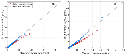
Following Kim et al. (2023), we use basin-averaged RF derived from all AORC grid points within the selected catchment areas. In addition, we want to leverage the long in situ observations to obtain more robust results from the statistical analysis. Rain gauges measure very local weather conditions. However, the assumption that such point RF quantities are uniformly distributed over the entire catchment could lead to mischaracterization of the flood hazard potential. Therefore, we apply a bias correction to the hourly RF gauge data to match the hourly basin-averaged RF quantities calculated from AORC. The quantile mapping method is used for the bias correction, fitting both hourly measured gauge data and hourly AORC basin-averaged data to gamma distributions. We follow the approach outlined in Smitha et al. (2018), which can be mathematically expressed as

$$\begin{array}{}\text{(1)}& {\mathrm{\text{RF}}}_{\text{Mod},x}=F_{\mathit{\gamma }}^{-\mathrm{1}}\left(F_{\mathit{\gamma }}\right({\text{RF}}_{\text{MS},x}\mathrm{|}{\mathit{\alpha }}_{\text{MS}},{\mathit{\beta }}_{\text{MS}}),\mathrm{|}{\mathit{\alpha }}_{\text{AORC}},{\mathit{\beta }}_{\text{AORC}}),\end{array}$$

where RF_Mod,x is the bias-corrected measured value of the original value RF_MS,x, and F_γ is the gamma distribution with α and β being scale and shape parameters. Figure 2 shows the quantile plots before and after the bias correction for the two study sites. The bias-corrected hourly measured RF data are then aggregated to obtain RF accumulation time series ranging from 1 to 48 h.

3.2 Extreme-event sampling and stratification

We define extreme events that can potentially cause compound flooding using the peak-over-threshold (POT) approach. The threshold selection is a subjective process. The threshold needs to be high enough to lead to a good fit of marginal distributions and low enough to capture a sufficiently large number of events to obtain robust estimates of the distribution parameters (i.e., bias-variance trade-off). Here, we set thresholds for NTR and RF time series such that we obtain five exceedances per year on average while using a 5 d declustering window (2.5 d before and after the event peaks) to ensure independence (Camus et al., 2021). We use the two-sided conditional sampling method outlined in Jane et al. (2020) and adopted in Kim et al. (2023). When conditioned on NTR, the maximum RF value within a 3 d window is selected, and the same procedure is followed when conditioning on RF. The sampling process is applied for all the RF accumulation time series from 1 to 48 h.

The identified POT events are stratified into two sets: events caused by TCs and events not caused by TCs. An event is assumed to have been caused by a TC if the center of circulation of a TC passed through a 350 km search distance from the center of the selected catchment within a time window of 3 d (2 d before and 1 d after) of a POT event. All other events are categorized as non-TC events. For Gloucester City, the threshold for NTR is set to 0.63 m, resulting in a total number of 580 POT events (that is consistent with five events per year on average). For RF, thresholds are set to obtain 580 POT events for each RF accumulation time from 1 to 48 h. After stratifying the POT events, 38 events are identified as TCs when conditioned on NTR and 43 when conditioned on RF, while the rest are non-TCs. For St. Petersburg, a threshold of 0.34 m is used for NTR to obtain 355 POT events, and the same number of POT events is obtained for each RF accumulation time. When conditioning on NTR (RF), 37 (47) events are identified as TC related.

To further sub-classify the non-TC events, we follow the same method using ETC track data but with a larger search radius of 1000 km in Gloucester City and 1200 km in St. Petersburg, reflecting the larger size of ETCs compared to TCs. The use of a 350 km radius for the TCs is likely to capture the large majority of TC-influenced events that generate extremes (Towey et al., 2022). The use of a 1000 or 1200 km radius for ETCs is likely to capture nearly all cases where ETCs are involved (e.g., Towey et al., 2018). This gives three classes of events: TC, ETC, and non-classified events. When conditioned on RF, the non-classified sample mainly includes convective RF events that are not related to cyclonic activity in the near atmosphere. When conditioned on NTR, the non-classified sample includes, for example, NTR events that could have still been induced by TCs or ETCs which passed outside the search radiuses. In the subsequent analysis, we first focus on the TC and non-TC events. We then quantify changes in the joint probabilities when excluding non-classified events.

3.3 Dependence analysis

We calculate Kendall's τ between NTR and RF for all RF accumulation times from 1 to 48 h to assess the sensitivity of the correlation to varying RF accumulation times (Kim et al., 2023). This is done in three ways: (a) all the POT events without stratification, (b) TC events, and (c) non-TC events. We find the RF accumulation time corresponding to the maximum correlation and use it for the bivariate analysis. To be consistent with the annual exceedance probability estimation process, a single RF accumulation time is selected in all stratified samples of a given study site.

Some regions along the US coast have experienced an increase in the correlation between RF and NTR since the mid-20th century (Wahl et al., 2015). Therefore, to assess temporal changes in the dependence, Kendall's τ is calculated for 30-year moving windows, shifted 1 year each time step (see Fig. 4). We assess the significance of temporal changes using the range of natural variability. The range is calculated as the 5th and 95th percentiles of Kendall's τ values obtained from randomly sampling 30 years of data for 10 000 iterations (Wahl et al., 2015). When a calculated τ value falls outside this range, the change is considered significant. The non-stationarity analysis is conducted using the selected RF accumulation time for each case study location.

3.4 Marginal distributions and joint probability analysis

Next, we identify the best-fitting marginal distributions for each set of stratified POT samples (TC and non-TC). The conditioning variables (both NTR and RF) are fit to the generalized Pareto distribution (GPD), which is most suitable for modeling POT extremes. When conditioning on NTR, the corresponding maximum RF sample is fit to various distributions with a lower bound at zero, and the best model is selected using the Akaike information criterion (Akaike, 1974). Here, the Birnbaum–Saunders, exponential, two-parameter gamma, three-parameter gamma, inverse Gaussian, lognormal, Tweedie, Weibull, two-parameter mixed gamma, and three-parameter mixed gamma distributions are tested. When conditioned on RF, the corresponding maximum NTR sample is fit to logistic and Gaussian distributions.

We use copulas to model the joint dependence between NTR and RF. According to Sklar's theorem (Sklar, 1959), the bivariate cumulative distribution F_XY(xy) of the variables X and Y, with univariate marginal distributions F_X(x) and F_Y(y) for all $(x,y)\in R^{\mathrm{2}}$, can be written as

$$\begin{array}{}\text{(2)}& F_{XY}(x,y)=C\left[F_X\right(x\left)F_Y\right(y\left)\right],\end{array}$$

where function C represents the bivariate copula on [0,1]. Annual exceedance probabilities (AEPs) can refer to different hazard scenarios (e.g., AND, OR, survival Kendall, structural) that define different geometries of upper sets that contain the events perceived as “dangerous” (Salvadori et al., 2016). Considering the recommendations of Moftakhari et al. (2019) for compound flood assessments, we use the AND scenario, which represents the exceedance of both X and Y. The joint AEP of a given pair of (x,y) is calculated as

$$\begin{array}{}\text{(3)}& {\displaystyle }\begin{array}{rl}{\text{AEP}}_{(x,y)}& =P(X>x\cap Y>y)/\mathit{\lambda }\\ & =(\mathrm{1}-F_X(x)-F_Y(y)+C_{XY}(xy\left)\right)/\mathit{\lambda },\end{array}\text{(4)}& {\displaystyle }{C}_{XY}\left(xy\right)=C\left[F_X\right(x),F_Y(y\left)\right],\end{array}$$

where λ is the average inter-arrival time between threshold exceedances. We consider 40 possible copula families and the independent copula using the VineCopula R package (Nagler et al., 2023) to identify the best-fitting copula family for each pair of samples. The most appropriate copulas are selected based on the Akaike information criterion.

After fitting the selected copulas to the stratified two-sided POT samples, the joint AEP of a given pair of (NTR, RF) can be calculated as follows:

$$\begin{array}{}\text{(5)}& {\displaystyle }\begin{array}{rl}{\text{AEP}}_{\left(\text{NTR,RF}\right)}^{\text{TC,con.NTR}}=& (\mathrm{1}-F_{\left(\text{NTR}\right)}^{\text{TC,con.NTR}}-F_{\left(\text{RF}\right)}^{\text{TC,con.NTR}}\\ & +C_{\left(\text{NTR,RF}\right)}^{\text{TC,con.NTR}})/{\mathit{\lambda }}^{\text{TC,con.NTR}},\end{array}\text{(6)}& {\displaystyle }\begin{array}{rl}{\text{AEP}}_{\left(\text{NTR,RF}\right)}^{\text{TC,con.RF}}=& (\mathrm{1}-F_{\left(\text{NTR}\right)}^{\text{TC,con.RF}}-F_{\left(\text{RF}\right)}^{\text{TC,con.RF}}\\ & +C_{\left(\text{NTR,RF}\right)}^{\text{TC,con.RF}})/{\mathit{\lambda }}^{\text{TC,con.RF}},\end{array}\text{(7)}& {\displaystyle }\begin{array}{rl}{\text{AEP}}_{\left(\text{NTR,RF}\right)}^{\text{non-TC,con.NTR}}=& (\mathrm{1}-F_{\left(\text{NTR}\right)}^{\text{non-TC,con.NTR}}\\ & -F_{\left(\text{RF}\right)}^{\text{non-TC,con.NTR}}\\ & +C_{\left(\text{NTR,RF}\right)}^{\text{non-TC,con.NTR}})/{\mathit{\lambda }}^{\text{non-TC,con.NTR}},\end{array}\text{(8)}& {\displaystyle }\begin{array}{rl}{\text{AEP}}_{\left(\text{NTR,RF}\right)}^{\text{non-TC,con.RF}}=& (\mathrm{1}-F_{\left(\text{NTR}\right)}^{\text{non-TC,con.RF}}-F_{\left(\text{RF}\right)}^{\text{non-TC,con.RF}}\\ & +C_{\left(\text{NTR,RF}\right)}^{\text{non-TC,con.RF}})/{\mathit{\lambda }}^{\text{non-TC,con.RF}},\end{array}\end{array}$$

where F is the marginal distribution, and C is the copula function. Following Bender et al. (2016) (and many other studies since then), we derive the combined AEP of a selected population (TC or non-TC) for a given pair of (NTR,RF) by taking the maximum AEP from the two conditioned samples.

$$\begin{array}{}\text{(9)}& {\displaystyle }{\text{AEP}}_{\left(\text{NTR,RF}\right)}^{\text{TC}}=\text{max}\left\{{\text{AEP}}_{\left(\text{NTR,RF}\right)}^{\text{TC,con.NTR}},{\text{AEP}}_{\left(\text{NTR,RF}\right)}^{\text{TC,con.RF}}\right\}\text{(10)}& {\displaystyle }\begin{array}{rl}& {\text{AEP}}_{\left(\text{NTR,RF}\right)}^{\text{non-TC}}\\ & =\text{max}\left\{{\text{AEP}}_{\left(\text{NTR,RF}\right)}^{\text{non-TC,con.NTR}},{\text{AEP}}_{\left(\text{NTR,RF}\right)}^{\text{non-TC,con.RF}}\right\}\end{array}\end{array}$$

3.5 Combining joint exceedance probabilities of two populations

The calculated AEPs from Eqs. (9) and (10) provide the joint AEPs for NTR and RF associated with the two populations, TC and non-TC, separately. However, both TC and non-TC events can create compound flooding in the same catchment. In the stratification process, a given POT event was categorized as caused by either TC events or non-TC events, thus making the probability distributions of these two populations independent of each other. Accordingly, the total annual non-exceedance probability (ANEP) of a given pair of (NTR,RF) can be calculated as follows:

$$\begin{array}{}\text{(11)}& {\displaystyle }{\text{ANEP}}_{\left(\text{NTR,RF}\right)}={\text{ANEP}}_{\left(\text{NTR,RF}\right)}^{\text{TC}}\times {\text{ANEP}}_{\left(\text{NTR,RF}\right)}^{\text{non-TC}},\text{(12)}& {\displaystyle }\begin{array}{rl}{\text{ANEP}}_{\left(\text{NTR,RF}\right)}=& \left(\mathrm{1}-{\text{AEP}}_{\left(\text{NTR,RF}\right)}^{\text{TC}}\right)\\ & \times (\mathrm{1}-{\text{AEP}}_{\left(\text{NTR,RF}\right)}^{\text{non-TC}}).\end{array}\end{array}$$

The associated return period (RP) is calculated as

$$\begin{array}{}\text{(13)}& {\text{RP}}_{\left(\text{NTR,RF}\right)}={\displaystyle \frac{\mathrm{1}}{\mathrm{1}-{\text{ANEP}}_{\left(\text{NTR,RF}\right)}}}.\end{array}$$

To perform the above calculations to generate joint probability isolines, the parametric space is discretized into small intervals along both NTR (${\text{NTR}}_{\mathrm{1}},{\text{NTR}}_{\mathrm{2}},\mathrm{\dots },{\text{NTR}}_i,\mathrm{\dots },{\text{NTR}}_n$) and RF (${\text{RF}}_{\mathrm{1}},{\text{RF}}_{\mathrm{2}},\mathrm{\dots },{\text{RF}}_j,\mathrm{\dots },{\text{RF}}_m$) axes, creating a mesh. AEPs on each point on this mesh are calculated for all pairs of (NTR_i,RF_j).

Although any combinations of NTR and RF along a given joint probability isoline have the same return probability, most hydrology-related engineering design approaches still rely on a single design event. Therefore, the “most-likely-event” strategy, introduced by Salvadori et al. (2011) and utilized in subsequent studies (e.g., Jane et al., 2020), is employed here. To quantify the relative probabilities of events along specific quantile isolines, we obtain 10⁶ combinations of NTR and RF by sampling from the fitted copulas, ensuring that the relative proportion of extremes is consistent with the empirical distribution. The relative probability along the isolines is then calculated by the kernel density function of the simulated sample. The location of the most likely event is assigned to the point with the highest relative probability density on an isoline (Salvadori and Michele, 2013).

3.6 Role of non-classified events

To assess the contribution of events that are non-classified, we repeat the same steps outlined above, stratifying the POT samples in four ways:

1. Both conditional samples are stratified as TCs and non-TCs.

2. The sample conditioned on RF is stratified as TC and ETC, and the sample conditioned on NTR is stratified as TC and non-TC.

3. The sample conditioned on RF is stratified as TC and non-TC, and the sample conditioned on NTR is stratified as TC and ETC.

4. Both conditional samples are stratified as TC and ETC.

More specifically, in (2) we omit the non-classified POT RF events (77 in Gloucester City and 192 in St. Petersburg), assuming that those are mainly convective events that are not captured, for example, by coarse general circulation models, and hence missing from compound flood assessments for future climates. In (3) we omit the non-classified POT NTR events (43 in Gloucester City and 105 in St. Petersburg), which could be caused by distant storms outside our search radius or, in the case of Gloucester City, could be influenced by high discharge in the Delaware River. In (4) we omit both types of non-classified events mentioned in (2) and (3).

To assess the impact of omitting different types of non-classified events in (2)–(4), we keep the calculated joint probability distribution of (1) as a reference and calculate the relative change in AEP along the probability isolines of (1). We also keep the copula family from (1) fixed for (2)–(4) to isolate effects unrelated to switching to a different copula; results for the same analysis but allowing for different copula families to be selected are shown in the supplementary material. We perform this analysis for the period from 1950 to 2021 where ETC tracks are available and both ETC and TC track data are more reliable.

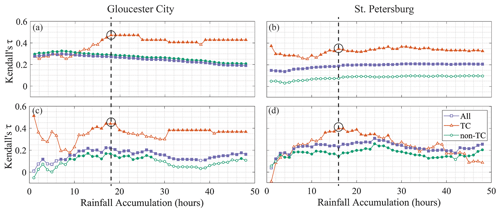
Figure 3 Kendall's τ between NTR and RF for different RF accumulation times for all events (purple), TCs (orange), and non-TCs (green) for samples conditioned on NTR (a, b) and RF (c, d). The filled markers indicate values that are significant at a 5 % level. The black circles with vertical dashed lines show the selected RF accumulation for each location.

4 Results

4.1 Dependence analysis

We use Kendall's rank correlation coefficient τ to calculate the strength of dependence between NTR and RF for different RF accumulation times. For both study sites, NTR and RF exhibit a weak but statistically significant correlation when considering all the POT events without any stratification (Fig. 3). However, when the events are caused by TCs, the correlation is stronger and varies with the RF accumulation time. Considering both conditioned samples, 18 and 16 h RF accumulation times are selected for the bivariate statistical modeling in Gloucester City and St. Petersburg, respectively.

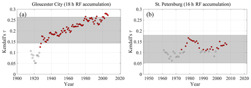
Figure 4 Changes in Kendall's τ between NTR and RF derived from a 30-year moving time window for (a) Gloucester City (18 h accumulation) and (b) St. Petersburg (16 h accumulation). Each circle represents the midpoint of the 30-year window. The red circles indicate significant correlation (α = 0.05). The horizontal grey bands represent the range between the 5th and 95th percentiles of natural variability.

When testing for non-stationarity in the dependence, we focus on the selected RF accumulation times. Figure 4 shows the changes in Kendall's τ between NTR and RF derived from a 30-year moving time window and the range of the natural variability of the correlation. We define the natural variability by randomly sampling 30 years many times (10 000 iterations were used) and calculating Kendall's τ for each sample. Figure 4a shows a significant change in τ during the last 3 decades in Gloucester City. A similar change is not detected for St. Petersburg, but the correlation values are more frequently significant during the late 20th and early 21st century (Fig. 4b). Therefore, to reflect current climate conditions and avoid underestimation of compounding effects, we use only the last 30 years of data to model the dependence structure at both study sites.

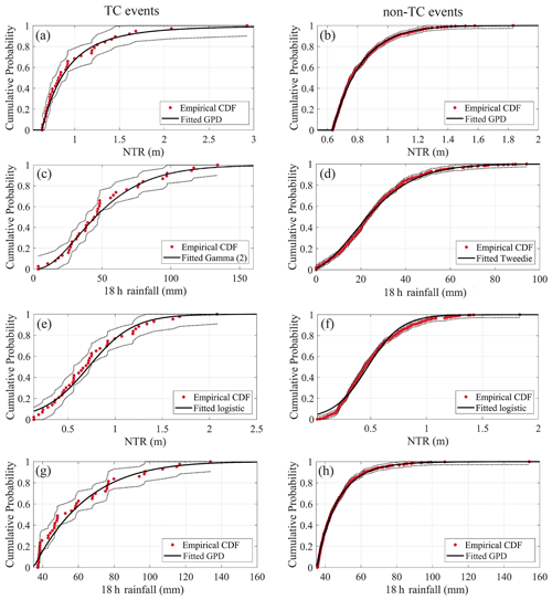
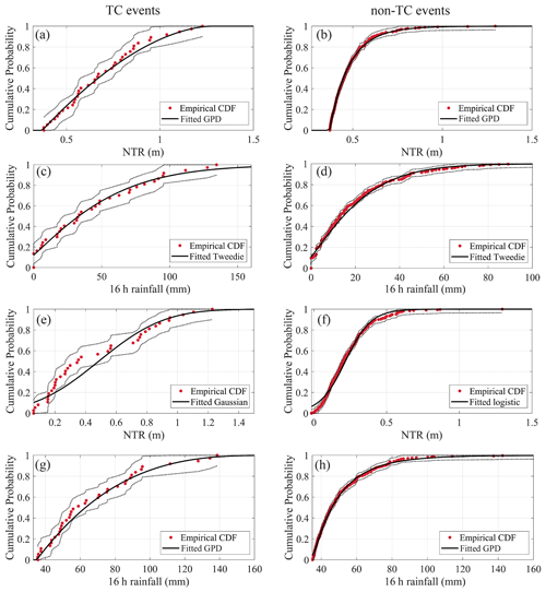
Figure 5 Selected parametric distributions compared to the empirical distributions of Gloucester City for TC events (left) and non-TC events (right). (a, b) NTR POT events when conditioned on NTR. (c, d) Maximum-RF events corresponding to NTR POT events when conditioned on NTR. (e, f) Maximum-NTR events corresponding to RF POT events when conditioned on RF. (g, h) RF POT events when conditioned on RF. The red dots represent the empirical cumulative distribution function (CDF) of the observations. The dashed lines denote the 95 % confidence intervals of the empirical CDF calculated using the Dvoretzky–Kiefer–Wolfowitz inequality.

Figure 6 The same as Fig. 5 but for St. Petersburg.

4.2 Bivariate statistical analysis

As described in Sect. 3.4, the conditioning variable is fit by a GPD, and for the conditioned variable several parametric distributions are tested. Selected distributions for each sample are indicated in Figs. 5 and 6 for the two study sites. The confidence interval of the empirical cumulative distribution function (CDF) is calculated using the Dvoretzky–Kiefer–Wolfowitz inequality (Dvoretzky et al., 1956).

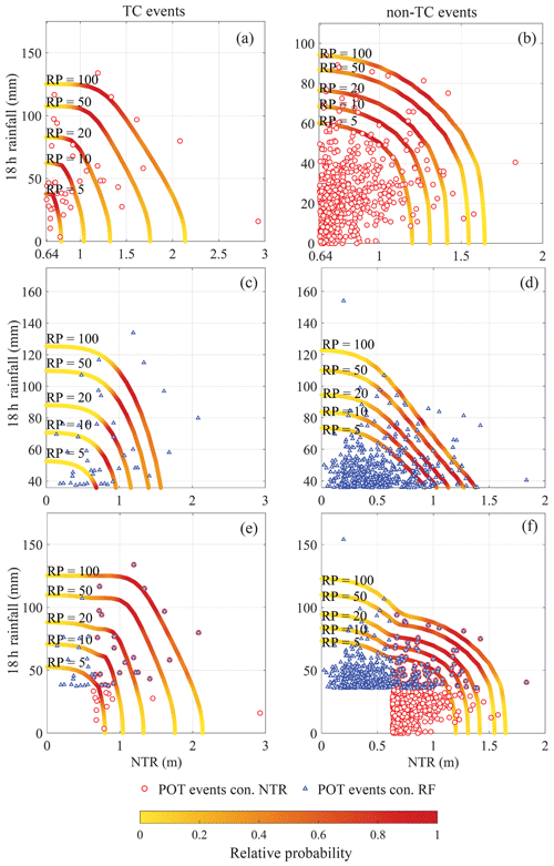
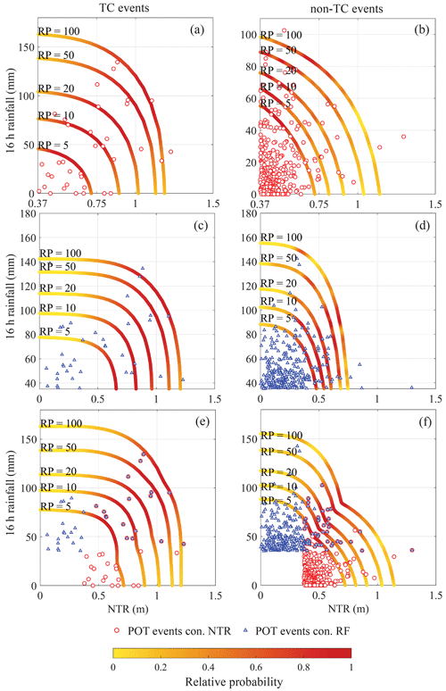
Figure 7 Results of bivariate statistical analysis for Gloucester City for TC events (left) and non-TC events (right) (a, b) when conditioning on NTR, (c, d) when conditioning on RF, and (e, f) when two conditioning samples are combined. Quantile isolines of the 5-, 10-, 20-, 50-, and 100-year joint return periods are shown where the color scale indicates the relative probability of events along the isolines. Note the different x- and y-axis scales for better clarity.

Figure 8 The same as Fig. 7 but for St. Petersburg, Florida.

The quantile isolines of 5-, 10-, 20-, 50-, and 100-year return periods are obtained for each conditional sample for the two study locations (Figs. 7 and 8). The number of events in the stratified samples and the selected copula models are shown in Table S1 in the Supplement. A relatively lower number of TC events are captured in both conditional samples compared to non-TC events (Table S1). The return periods of events with extreme NTR and non-extreme RF are relatively lower (the AEP is higher) when they are caused by TCs compared to non-TCs. When the samples are conditioned on RF, events with extreme RF and non-extreme NTR show nearly the same return periods in both populations (Figs. 7c, d and 8c, d).

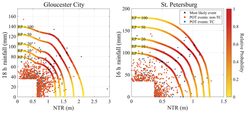
Figure 9 Joint probability isolines for the two study sites after combining the AEPs of the two populations (TC and non-TC). The color scale indicates the relative probability of events along the isolines. The location of the most likely event is assigned to the point with the highest relative probability density on an isoline.

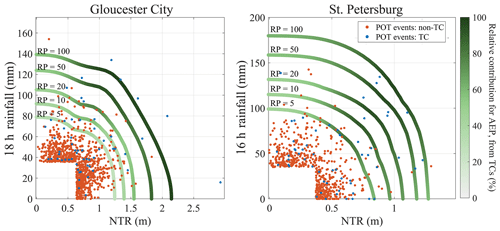
Figure 10 Relative contribution of TCs to the AEP along the joint probability isolines for the two study locations. The color scale indicates the ratio of AEP associated with TCs to the combined AEP of both populations.

The quantile isolines after combining the joint probability distributions of the two storm type populations (TC and non-TC) are shown in Fig. 9. To quantify the relative contribution from each of them, we calculate the ratio of AEP contributed by TCs to the total AEP along the isolines (Fig. 10). In Gloucester City, more than 60 % of the AEP of low-probability events (i.e., events with return periods above 50 years) is associated with TC events, while more than 70 % of the AEP of high-probability events (i.e., events with return periods below 20 years) is associated with non-TCs. In St. Petersburg, when both NTR and RF are extreme, TCs mainly drive the joint AEP. For example, TCs contribute over 90 % to the AEP of events with more than 100 mm 16 h RF and 0.8 m NTR. Closer to the axes (either extreme NTR or extreme RF), both types of events contribute approximately evenly to the joint AEP for rare events. For both locations, the region with extreme RF and non-extreme NTR shows a major contribution of non-TCs to the AEP.

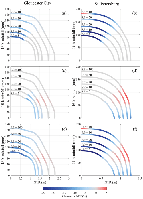
Figure 11 Change in AEP of the combined populations in Gloucester City (a, c, e) and St. Petersburg (b, d, f) (a, b) when omitting the non-classified POT RF events, (c, d) when omitting the non-classified POT NTR events, and (e, f) when omitting all non-classified events. The change in AEP was calculated along the joint probability isolines derived for the analysis where events are stratified as TC and non-TC.

4.3 Role of non-classified events

To assess the role of non-classified events, such as convective RF events and surge events caused by remote cyclones, we repeat the above analysis as outlined in Sect. 3.6. The calculated relative changes in AEP along the joint probability isolines after combining the AEPs of the two populations are shown in Fig. 11. When removing non-classified POT RF events (those are mainly convective events), the AEP decreases for events where RF is extreme and NTR is small to moderate (Fig. 11a and b). This becomes more noticeable for events with higher AEPs (i.e., events with return periods below 10 years), especially in St. Petersburg where they reach up to 25 % reduction. However, in Gloucester City, this impact becomes negligible for rare events (i.e., events with return periods above 50 years). When the non-classified POT NTR events (e.g., caused by remote cyclones) are removed from the analysis, the AEP decreases slightly for events where NTR is extreme and RF is small, while the AEP increases slightly when NTR is extreme and RF is moderate (Fig. 11c and d).

As mentioned in Sect. 3.6, we assume that the copula types that are used for the previous analysis (with events stratified as TC and non-TC) remain the same after removing non-classified events. We also conducted the analysis while allowing the selected copulas for the different conditional samples to change (see Fig. S1 in the Supplement and Table S2 in the Supplement). When allowing copulas to change, the changes in the AEPs along the isolines become more pronounced in Gloucester City when removing the non-classified POT NTR events. For example, they increase up to 35 % for the events where NTR is extreme and RF is moderate (Fig. S1e).

5 Discussion

5.1 Dependence analysis

The strong correlation between NTR and RF when the events are caused by TCs (see Fig. 3) suggests that there is a higher potential for compound flooding by TCs in both study sites. This can be attributed to the nature of TCs, notably their propensity for extreme-RF potential combined with strong winds. The non-TC samples in our analysis contain all events that are not directly linked to a TC (e.g., ETCs or convective events) and show weak but stable (over different rainfall accumulation times) correlation between NTR and RF. The stronger TC correlation is in line, for example, with findings reported by Kim et al. (2023) for the Dickinson Bayou watershed in Texas. However, they reported weak and insignificant correlation throughout all RF accumulation times (1 to 48 h) for non-TC events when conditioning on NTR. For Gloucester City the same conditional sample shows a slightly higher and significant correlation for all RF accumulation times (see Fig. 3). When the events are not stratified and treated as a single population, the correlation is similar to the one found for non-TCs, leading to an underestimation of the compound flood potential. These results highlight the importance of differentiating between storm types associated with different physical processes and characterizing their individual contributions to compound flood potential. By selecting an RF accumulation time that leads to the maximum correlation, we account for the sensitivity of correlation to RF accumulation time while following a conservative approach that avoids underestimating the dependence and compound flood potential.

5.2 Combining joint exceedance probabilities of two populations

Prior studies have only focused on merging the AEPs of two populations within a univariate framework (e.g., Orton et al., 2020). Our proposed methodology combines the AEPs of two populations in a bivariate framework that also has the flexibility to be further expanded to account for three or more populations. The joint probability distributions (Fig. 9), as determined by combining the AEPs of two populations, provide insights into the compound flood potential at each of the study sites. The framework derives a single isoline for each return period, which can be used, for example, to derive a single most likely design event (Salvadori et al., 2011, 2013). For Gloucester City, for instance, the most likely 100-year design event (i.e., the event with the highest relative probability along the 100-year isoline) is given by 1.60 m NTR and 87 mm 18 h RF. Under the assumption of independence between NTR and RF, the same event has a return period of 196 years. It should be noted that the Philadelphia tide gauge is located along the Delaware River (see Fig. 1), and the recorded water levels are influenced by both wind-driven storm surge and river discharge. In this study, we do not explicitly account for wind-driven surge and river discharge separately (NTR incorporates both), but the framework presented here is flexible enough to be extended for this purpose, e.g., by including NTR from an open-coast tide gauge near the Delaware River mouth and an upstream stream gauge. The most likely 100-year design event for St. Petersburg is comprised of 1.02 m NTR and 117 mm 16 h RF under the independence assumption that the return period of the same event increases to 156 years.

The magnitude of the univariate 100-year 18 h RF event is (after combining the AEPs of the two populations) 139 mm for Gloucester City and 180 mm for St. Petersburg (see Fig. 9). This is approximately an 11 % increase compared to the univariate 100-year 18 h RF of the TC samples at each site (125 and 163 mm). For the univariate 5-year 18 h RF the increase is 49 % in Gloucester City (from 53 to 79 mm) and 34 % in St. Petersburg (from 78 to 99 mm) (Fig. 9).

The return levels for RF are similar for the TC and non-TC samples, but TCs lead to higher NTR return levels, particularly in Gloucester City (see Fig. 10). This implies that the most extreme surges are caused by TCs, but both TC and non-TC events can produce similar rainfall totals. These results indicate that relying solely on TCs may be inadequate when analyzing compound flood risk in coastal catchments that are also exposed to other storm types. TCs are most relevant for events with low AEPs, which are important for flood zoning and critical infrastructure design. ETCs, on the other hand, mainly drive compound flood potential for events with higher AEPs, which are most relevant, for example, for stormwater management and design.

5.3 Role of non-classified events

As described in Sect. 3.6, the analysis was repeated to assess the impact of non-classified events. This includes, for example, NTR events caused by remote storms outside our pre-defined search radiuses, NTR in Gloucester City that is caused by high river discharge, and convective RF events. This is important because when studying future compound flooding, we typically rely on general circulation models, which do not capture convective RF events. Similarly, remotely triggered NTR events may be missed in assessments where only cyclones that pass through a defined region are included. Our analysis sheds light on the relative importance of those types of events in addition to TCs and ETCs that directly affect the area of interest.

Neglecting RF events that are likely locally generated can lead to an underestimation of the overall AEP (or overestimation of the return period), particularly for more frequent events (i.e., events with return periods below 10 years) (see Fig. 11a and b). This can be attributed to the nature of locally generated convective RF events since they are generally less intense in magnitude but occur with a greater frequency compared with TCs and ETCs. The reduction in AEP is also higher in St. Petersburg where 55 % (192 events) of the RF events exceeding the threshold are not linked to ETCs or TCs. This highlights the importance of convective RF events in St. Petersburg and thus the need for high-resolution models to characterize future flood hazard potential.

Removing non-classified events where NTR exceeded the threshold from the analysis leads to a slight reduction in AEP for events where NTR is extreme and RF is small and to a slight increase in AEP where NTR is extreme and RF is moderate (see Fig. 11c and d). This increase in AEP is potentially caused by the fact that the non-classified events have weaker correlation between NTR and RF compared to ETCs and TCs; hence, excluding them leads to larger joint AEPs. In the specific case of Gloucester City, those non-classified events can also include high-discharge events in the Delaware River, leading to high water levels (and hence high NTR) at the Philadelphia tide gauge.

Overall, excluding non-classified events leads to smaller changes in the joint probabilities in Gloucester City compared to St. Petersburg, especially when focusing on rare events (i.e., events with return periods above 50 years) (see Fig. 11e and f). This is likely because of the proximity of Gloucester City to the US East Coast where ETCs are more frequent and the overall number of non-classified events is lower (77 when conditioned on RF, 43 when conditioned on NTR).

One limitation of the proposed framework is the identification of compound events based on extreme flood drivers. In some locations, none of the flood drivers need to be extreme to cause compound flooding, as geographical exposure and other factors (e.g., elevation, drainage, permeability) play dominant roles. Therefore, the focus here is on assessing the compound flood potential and how the joint probabilities of different flood drivers are linked to various storm types. To extend the proposed framework to fully characterize the compound flood risk, the statistical approach can be combined with hydrodynamic numerical models (so-called hybrid modeling, e.g., Moftakhari et al., 2019) to estimate flood inundation. However, analyzing only the most likely event (even though it may be the most plausible given the observations) does not capture the range of flood levels that could be generated by different combinations of flood drivers (NTR and RF) along an isoline. One way to address this limitation is to sample an ensemble of events (peak NTR–RF combinations) along the isoline and run them through flood models. Alternatively, a response-based approach can be employed, which involves simulating flood hazard for a large number of synthetic events from the multivariate statical model and then performing the statistical analysis on the response variable of interest (e.g., flood depth at a given location). The latter is computationally demanding, possibly necessitating the use of a surrogate model; however the return level estimates are likely to be more robust than when adopting an event-based approach (Jane et al., 2022a). The simulated probabilistic flood depths and extents can then be incorporated with exposure and vulnerability data to perform a comprehensive flood risk assessment.

Additionally, despite the long data records used (Gloucester City, 1901 to 2021, and St. Petersburg, 1948 to 2021), the stratified TC samples contain a relatively small number of events due to their rare occurrence in historical observations. When the framework is applied to a different site with less data, the smaller sample size may result in higher uncertainty in modeling the upper tail of the NTR and RF distributions. This limitation can be addressed by combining the proposed framework with synthetic flood driver information derived from physics-based models (e.g., Gori et al., 2020).

6 Conclusions

This paper introduces a flexible copula-based statistical framework to assess compound flood potential from multiple drivers while explicitly accounting for different storm types. Here we apply the method to two case study sites, Gloucester City, New Jersey, and St. Petersburg, Florida, which are exposed to different storm climatologies. Our study highlights the importance of differentiating between storm types with different physical processes and characterizing their individual contributions to compound flood potential. Overall, we find that TCs modulate the tails of the joint distributions (events with higher return periods), while non-TC events have a strong effect on events with low to moderate joint return periods. While the most extreme events and associated probabilities are most relevant for flood zoning and critical infrastructure design, more moderate events are crucial, for example, for stormwater management and design. We also quantify how non-classified storms that are not linked to either TCs or ETCs in the region impact the compound flood potential. The results differ across study sites with the effects being overall smaller in Gloucester City than in St. Petersburg, and they also affect different parts of the joint distribution differently. This is important because assessments of future compound flood hazard (and flood hazard in general) typically rely on the output from general circulation models that may not capture such events due to their coarse resolution. This can in turn lead to a misrepresentation of flood hazard and risk. Our results provide insights into how large (or small) the effect is of not capturing all relevant storm types when studying compound flooding. The method is flexible so that additional storm types (e.g., storms with certain tracks or other characteristics) can be identified and their effect on compound flood potential can be quantified. Finally, while we focus on observed data and their derivative products, the framework can be used with model output data including hindcasts or future projections.

The focus here is on the compound flood potential and how the joint probabilities of different flood drivers are linked to different storm types. However, the combined probability distributions of the different populations can also be used to generate a large number of synthetic events that can act as boundary conditions for hydrodynamic numerical models to fully characterize compound flood hazard, including flood depths and extent. This will be demonstrated in a separate study.