Strategies for comparison of modern probabilistic seismic hazard models and insights from the Germany and France border region

The latest generation of national and regional probabilistic seismic hazard assessments (PSHAs) in Europe presents stakeholders with multiple representations of the hazard in many regions. This raises the question of why and by how much seismic hazard estimates between two or more models differ, not only where models overlap geographically but also where new models update existing ones. As modern PSHA incorporates increasingly complex analysis of epistemic uncertainty, the resulting hazard is represented not as a single value or spectrum but rather as probability distribution. Focusing on recent PSHA models for France and Germany, alongside the 2020 European Seismic Hazard Model, we explore the differences in model components and highlight the challenges and strategy for harmonising the different models into a common PSHA calculation software. We then quantify the differences in the source model and seismic hazard probability distributions using metrics based on information theory, illustrating their application to the Upper Rhine Graben region. Our analyses reveal the spatial variation in and complexity of model differences when viewed as probability distributions and highlight the need for more detailed transparency and replicability of the models when used as a basis for decision-making and engineering design.

1 Introduction

Effective mitigation of seismic risk, be it at a local, national, or regional scale, requires a quantitative assessment of not only the strength or impacts of the perils an area may be subjected to, but also their probability of occurrence over a given time frame. For earthquakes, probabilistic seismic hazard assessment (PSHA) is now established as the primary means through which our understanding of the physical phenomena is translated into a framework that can yield critical information of relevance for engineering design, urban planning and development, and financial instruments to mitigate the economic impacts of these events on society. Given the volume of information for risk mitigation that PSHA can produce, national- and regional-scale PSHA models are now available for every country across the globe (Pagani et al., 2020), with many countries now having developed several successive generations of seismic hazard models and, in some regions, multiple models offering different perspectives on seismic hazard for the same area of interest (Gerstenberger et al., 2020).

The issue of multiple perspectives on seismic hazard in a region can be an important one to address from the point of view of model developers, but it also has significant implications for the users of the seismic hazard outputs. In the case that a new seismic hazard model for a region is produced that is intended to update or supersede an existing model, there may be recognition that new data for that region and/or developments in PSHA practice justify revising or updating a seismic hazard model periodically, although this revision will inevitably have implications for stakeholders, particularly when hazards are found to increase or decrease substantially at a location as a result of the new information. In Europe, many different countries are confronted with this situation as new generations of national seismic hazard models emerge. There is, however, also a compounding issue, which is the need for pan-European assessments of seismic hazard. Two major models within the last decade have resulted from large-scale multi-institution projects that have put a strong focus on incorporating state-of-the-art developments in PSHA, namely the 2013 European Seismic Hazard Model (ESHM13) (Wössner et al., 2015) and the 2020 European Seismic Hazard model (ESHM20) (Danciu et al., 2021).

Since the completion of ESHM13, many new seismic hazard models have been developed at national scale, among which are Switzerland (Wiemer et al., 2016), Spain (IGN, 2017), Türkiye (Akkar et al., 2018), Germany (Grünthal et al., 2018), France (Drouet et al., 2020), Italy (Meletti et al., 2021), the UK (Mosca et al., 2022), and many more. Furthermore, in other countries such as Portugal and Greece, although no new national seismic hazard model has been developed, ESHM13 was instrumental in prompting efforts to collect and improve geophysical datasets as an initial step toward new seismic hazard models in these countries in the future. In many cases, it has been possible to leverage these efforts within the model development process of ESHM20. Several factors have motivated these national-scale developments, but chief among these is the establishment of Eurocode 8 (EC8; CEN, 2004) as the predominant standard covering earthquake-resistant design. EC8 devolves some specific components of its seismic design requirements to each of the participating member states via their respective national annexes. Among these components are the seismic hazard map on which the design levels of seismic input are based. In many cases, national building design authorities have opted to undertake revisions to their national seismic hazard maps, in part aiming to bring these into line with (or even exceeding) standards for state-of-practice PSHA modelling in Europe set by ESHM13 but also because new or more detailed data may be available at local scale to allow for a refined estimate of hazards that may not be scalable to larger multi-national regions. These national models should form the authoritative reference seismic hazard model for application to engineering design in their respective countries. In some cases, however, these models have integrated components or ideas developed within ESHM13. We also expect this trend to continue with expected updates to Eurocode 8 and following the publication of ESHM20.

The dual existence of both a regional-scale model (or models) and a national model that cover the same territory raises the question of comparison between models. How and why do models differ and how can we quantify differences? It has become standard practice for modern seismic hazard assessment to contain detailed assessments of epistemic uncertainty in both the seismogenic source model (SSM) and the ground motion model (GMM) components. These are incorporated into the analysis in the form of logic trees, which generate many seismic hazard curves by enumerating (or sampling) combinations of alternative models or model parameterisations and their associated weights. Logic trees have been adopted as the standard tool for epistemic uncertainty assessment in site-specific PSHA for several decades, yet at national and/or regional scales the latest generation of European seismic hazard models is only the second generation to consider epistemic uncertainties as standard practice. The increase in the sophistication and complexity of the logic trees between the first and second generations is considerable. A clear example of this can be found in the national seismic hazard models of Switzerland, which in the previous-generation model contained 72 logic tree branches, with no more than two or three different models capturing epistemic uncertainties in the seismogenic source, the magnitude frequency distribution, and the GMM (Giardini et al., 2004), while the 2015 update boasts more than 1 million logic tree branches describing epistemic uncertainties on a much greater range of source and ground motion parameters (Wiemer et al., 2016). A similar development can be seen in Italy, where the 2004 national seismic hazard map (MPS04, Stucchi et al., 2011) was based on a logic tree of only 16 branches, while MPS19 (Meletti et al., 2021) contains between 33 and 7986 branches depending on whether earthquake hazard at a location is affected by subduction and/or volcanic earthquakes in addition to the shallow crustal seismicity. With comprehensive treatment of epistemic uncertainty now standard in models, the breadth and definition of outputs from PSHA mean that we cannot quantify differences purely in terms of an increase or decrease on a map in peak ground acceleration (PGA) with a 10 % probability of exceedance (PoE) in 50 years, but rather we need to consider the differences in terms of distributions of hazard from the epistemic uncertainty analysis and do so across the range of outputs.

This paper aims to illustrate the full depth of what we mean by comparison of PSHA models by focusing on three recent models that overlap with one another in terms of the territory covered: (1) the 2016 national seismic hazard model for Germany prepared by Grünthal et al. (2018), (2) the PSHA model for metropolitan France by Drouet et al. (2020), and (3) the 2020 European Seismic Hazard Model (ESHM20). These models and the overlapping area in question are of particular interest to us for several reasons. Firstly, the area of overlap for the three models corresponds to the Upper and Lower Rhine region, one of the most populated and economically productive regions of Europe with high economic and human exposure (Crowley et al., 2021), meaning that differences in the characterisation of seismic hazard and its uncertainty may result in significant differences in terms of economic risk or risk to life. In both France and Germany, successive and/or alternative seismic hazard models have prompted discussions among the scientific and engineering communities in both countries as to the causes of differences between models, their interpretation, and their implications for risk and/or engineering design. In this case, however, each model adopts a complex logic tree to describe the epistemic uncertainty in seismic hazard, and as such they illustrate the challenges faced in understanding and interpreting differences between models developed according to the current state-of-practice standards in PSHA.

We begin with a general overview of the three models in Sect. 2, highlighting both the common elements in the models and the critical differences. As each model uses a different PSHA calculation engine, we have endeavoured to translate both the French and the German hazard models from their original proprietary software into the open-source OpenQuake engine, which allows us to explore the models in detail, affording us more control over the calculation and better understanding of the detailed modelling differences that the PSHA software can introduce. Section 3 therefore describes the motivations for translating the models across to another software and some of the lessons learned from this process. With the models implemented into a common PSHA software, we outline various quantitative techniques to explore the differences between them, firstly in terms of the spatial variation in the distribution of activity rates (Sect. 4) and then by looking at the differences in the hazard outputs for the three models in the France–Germany border region (Sect. 5). An overview of the extent of the France–Germany border region and the geographical features of relevance mentioned in this article can be seen in Fig. 1. We conclude with recommendations on how to approach model-to-model comparison based on insights gained from our experience. An additional set of notes has been compiled that expands upon certain topics mentioned in the current paper, which can be found in the Supplement.

We hope these recommendations may form a useful reference point for end users of these models when considering how and why PSHA models for a given region can differ and how to use this information to form a basis for decision-making when it comes to adopting models or migrating from one to another for use in application.

2 Overview of the recent PSHA models for Europe, France, and Germany

The first seismic hazard model considered here is the 2016 national seismic hazard model of Germany (DE2016 hereafter), which was prepared by Grünthal et al. (2018) on behalf of the Deutsches Institut für Bautechnik (DIBt) with the aim of providing an up-to-date seismic zonation for the current design code and national annex to Eurocode 8 (E DIN EN 1998-1/NA:2018-10, 2018). Among the developments included in DE2016 is a new earthquake catalogue for Germany and the surrounding regions that updates the previous European-Mediterranean Earthquake Catalogue (Grünthal and Wahlström, 2012), seismogenic source and ground motion model logic trees, and a novel rigorous approach to characterise uncertainty in the magnitude frequency distribution. The PSHA model covers the entire national territory of Germany (plus a small band outside the national borders) with hazard curves calculated every 0.1° latitude and longitude, resulting in seismic hazard curves at 6226 locations across the country for PGA and spectral accelerations for periods in the range of 0.02 and 3.0 s. Hazard curves are calculated on a reference site condition of V_S30 800 m s⁻¹.

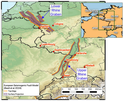
Figure 1 Extent of the France–Germany border region with the main locations of interest for this study marked. Active faults shown for the Lower Rhine Graben and Upper Rhine Graben are taken from the ESHM20 seismogenic fault model and the European Database of Seismogenic Faults (Basili et al., 2023).

The second seismic hazard model we consider is that of Drouet et al. (2020), which covers the whole of metropolitan France (FR2020 hereafter) and was developed to capitalise on the outcomes of preceding research into seismic hazard emerging from the SIGMA project (Pecker et al., 2017). New developments included an updated magnitude-homogeneous earthquake catalogue (FCAT-17, Manchuel et al., 2018), recently developed ground motion models (GMMs) for France (Ameri, 2014; Ameri et al., 2017; Drouet and Cotton, 2015), and refinements to the characterisation of seismic sources and magnitude frequency relations (MFRs) that built on innovative approaches adopted in the eastern United States (EPRI, 2012). The hazard model is produced assuming a site condition of V_S30 800 m s⁻¹ (Eurocode 8 Class A), with hazard curves calculated at 6836 sites for PGA and spectral acceleration with periods in the range of 0.01 to 3 s.

The 2020 European Seismic Hazard Model (ESHM20) is the latest-generation seismic hazard model for Europe, covering 36 countries from Iceland in the northwest to Türkiye in the southeast. As a comprehensive and state-of-the-art multi-national-scale model that has built on new data and scientific developments since ESHM13, ESHM20 provides a comprehensive set of seismic hazard curves, hazard maps, and uniform hazard spectra calculated at more than 100 000 locations, including the whole of continental Europe, the UK, and Ireland, as well as Iceland and various islands in the Mediterranean and Atlantic. ESHM20 not only is the basis for the seismic input parameter maps of S_α and S_β (the short- and long-period coefficients anchoring the elastic design spectrum) that will form an informative annex to the forthcoming Eurocode 8, but also provides the seismic hazard input into the 2020 European Seismic Risk Model for Europe (Crowley et al., 2021). For Eurocode 8, seismic hazard is calculated with respect to the reference soil condition of V_S30 800 m s⁻¹ (assuming depth to the V_S 800 m s⁻¹ layer of less than 5 m), which is consistent with both FR2020 and DE2016.

Our comparison of the models begins at the level of the model components. At the first level this comprises the seismogenic source model(s) and the ground motion model(s), but we subsequently deconstruct the former into elements relating to the delineation of the sources and the calculation and representation of earthquake recurrence in the logic tree. The respective logic trees of our three hazard models (DE2016, FR2020, and ESHM20) all implement branch sets to capture epistemic uncertainty in each of these components. An overview of the components of the three models and how they approach the characterisation of each aspect and its epistemic uncertainty can be seen in Table 1. The complete logic trees are shown for DE2016, FR2020, and ESHM20 in Figs. 2, 3, and 4 respectively.

Table 1 Comparison of seismic hazard model components for each of the three models (DE2016, FR2020, and ESHM20).

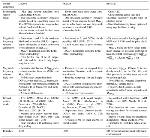
Figure 2 Complete logic tree of seismogenic source models (a) and ground motion models (b) for DE2016 (Grünthal et al., 2018).

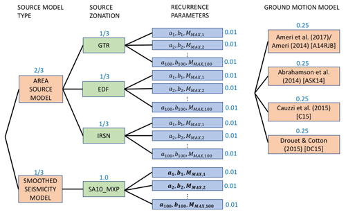
Figure 3 Complete logic tree for France (Drouet et al., 2020) containing both the seismogenic source model and the ground motion model.

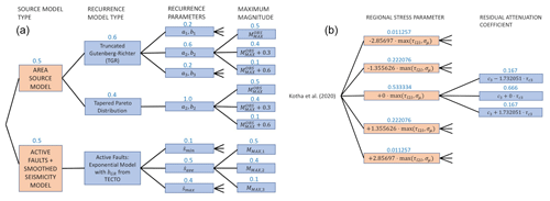
Figure 4 Complete logic tree of seismogenic source models (a) and ground motion models (b) for ESHM20 (Danciu et al., 2021).

2.1 Representation of the seismic source

As our focus is on Germany and France, we work in areas of primarily low to moderate seismicity and low tectonic deformation. Although active faults have been mapped in certain areas, most notably the Lower Rhine Graben (Vanneste et al., 2013), not all the assessments have aimed to represent these explicitly in the seismic source models or they have only chosen to do so in some branches. An active fault in the current context can be defined as a fault that is capable of generating earthquakes with M≥5.5 and with a non-zero minimum bound on the slip rate (e.g. Danciu et al., 2021). As such, the distribution of active faults is limited only to the fastest-slipping and most well constrained structures in and around the Rhine Graben, and each set of seismogenic source models principally comprises area source zones and/or gridded seismicity zoneless sources. These types of sources are known as distributed seismicity sources, and earthquake recurrence is modelled mostly by a double-truncated Gutenberg–Richter model whose parameters, a, b, COV(a,b), and maximum magnitude (M_MAX), are constrained by fit to observed seismicity in each zone. The area zonations of the three models can be found in the Supplement Part A Sect. S1.

DE2016 adopts five alternative area source zonations (Models A, B, C, D, and E) alongside two zoneless smoothed seismicity models. For the area sources, Grünthal et al. (2018) explicitly formulate their logic tree as a combination of large-scale area source zones (LASZs) and small-scale area source zones (SASZs). Models A and B are LASZs, which assume that the regional-scale tectonics are the main factors delineating the seismic sources and that seismicity may be uniform across large areas when viewed at longer timescales than those captured by the observed seismicity. Models C to E are SASZs, which regard local-scale seismicity and geological features as the primary guide to the seismogenic sources and therefore delineate smaller-scale zones. The smoothed seismicity branches differ in approach from those found in both FR2020 and ESHM20, which use a smoothing kernel with an adaptive bandwidth but for which the bandwidth is calibrated on the local density of seismicity (e.g. Helmstetter and Werner, 2012). Instead, DE2016 uses an adaptive kernel with a magnitude-dependent bandwidth based on the method of Woo (1996). The two branches are equally weighted and consider the two cases in which the bandwidth is capped at 25 km (H(m)≤25 km) and one in which it is unconstrained (H(m)≤∞). One feature of note among the SASZ models is that Model C adds explicit active fault sources in the Lower Rhine Graben (LRG). These adopt the fault geometry proposed by Vanneste et al. (2013) but use observed seismicity with M≥5.3 across two catchments (area sources) to constrain long-term seismic activity rates for the faults. The seismic activity rates for M≥5.3 within the two catchments are distributed among the faults within the catchments according to their respective fault length, while for M<5.3 the catchments are treated as area sources. This combined area and fault source model receives the highest weighting of the five source models.

FR2020 adopts three area source zonations, which assimilate those implemented in previous studies by different organisations: Geoter (now Fugro) (GTR), Électricité de France (EDF), and the Institut de Radioprotection et de Sûreté Nucléaire (IRSN). In addition, a single zoneless source model branch is included, which is developed using smoothed seismicity with an adaptive kernel bandwidth applied to the observed seismicity in France from 1960 to 2017. The smoothed seismicity produces seismic sources in the form of 10 km × 10 km cells, with the activity rate (a value) varying cell by cell but the b value and M_MAX calculated based on the location of the cell with respect to a set of superzones, i.e. large-scale area zones delineating tectonically based domains (Grands Domaines).

The seismogenic source model of ESHM20 follows a different approach to that of either FR2020 or DE2016. In terms of the number of different source models considered, the source model branch set is simpler. It contains one branch of exclusively area source zones and another branch for a combined smoothed seismicity and active fault model. As described in Danciu et al. (2021), the area source model aims to unify existing area source zonations from different national PSHA models across Europe, modifying the source geometries at the boundaries of models to ensure a seamless transition from one region to another. In the France–Germany region, the unified area source model adopts DE2016's Model C as its basis in Germany and the IRSN source model branch of FR2020 for France, alongside existing models from Belgium, Switzerland (Wiemer et al., 2016), and the UK (Mosca et al., 2022). The active fault and smoothed seismicity model includes explicit characterisation of faults in both the Upper and the Lower Rhine Graben regions, as well as numerous faults in France adapted from the dataset of Jomard et al. (2017). Information regarding the dataset of active faults can be found in Basili et al. (2023). Smoothed seismicity is characterised using an isotropic power law kernel with adaptive bandwidth, whose parameters are optimised using log-likelihood scoring (Nandan et al., 2022). To combine the smoothed seismicity with the active faults, a buffer zone is defined for each fault, within which magnitudes lower than a fault-size-dependent threshold are kept as smoothed seismicity, while magnitudes larger than the threshold are associated with the fault surface. For regions away from the fault, the b value and M_MAX are based on values determined from area sources in a large-scale zonation, reflecting regional-scale tectonics (named TECTO). More information on the relevance of this is seen in Sect. 2.2.

In this first component we can see that the three PSHA models display both similarities and differences in their approach to characterising epistemic uncertainty in the seismogenic source model. FR2020 and DE2016 aim to represent uncertainty in the sources predominantly through multiple uniform area zonations, while ESHM20 divides its weights more evenly between two different source typology definitions. Though only DE2016 explicitly adopts the LASZ/SASZ characterisation, this same philosophy is present in FR2020's Grands Domaines model and ESHM20's TECTO model. In the FR2020 model the distinction between large- and small-scale zone models within the three zonations considered (GTR, EDF, and IRSN) is not as clear and intentional as it had been for DE2016. Where the contrast exists, it manifests mostly in the difference between the IRSN and EDF models (46 and 49 zones respectively) and the zonation provided by GTR (92 zones). Each of these three models could be described as delineating zones accounting for both geology and seismology, albeit in proportions that are difficult to define. Only DE2016 models the LASZ explicitly in its A and B source zonations; however, all three models will come to adopt similar approaches toward earthquake recurrence by using their LASZ as a basis for fitting their earthquake recurrence models, which may then inform (either by direct calibration or as a prior distribution) the MFRs for the small-scale area sources with few events. In that sense, their philosophies toward area zonation are similar, but their implementation differs.

Adaptive kernel smoothed seismicity source models are present in all respective logic trees, though each PSHA model has taken a different approach to characterisation and implementation. Both FR2020 and ESHM20 have used approaches similar to that of, for example, Helmstetter and Werner (2012), optimising the parameters controlling the adaptive kernel's bandwidth using log-likelihood analysis applied to a pseudo-prospective seismicity forecast. However, the models arrive at significantly different outcomes in terms of the spatial distribution of activity rate. DE2016 adopts a different approach by using magnitude-dependent adaptive kernels, which increase the bandwidth for larger magnitudes, meaning that the rate in many low-seismicity regions is dominated by activity from the most extreme events. This contrasts with the adaptive bandwidth methods used in FR2020 and ESHM20 for which the bandwidth is based on the density of seismicity. For FR2020 and DE2016 the total weight assigned to the smoothed seismicity branches is the same (0.25), while for ESHM20 the combined seismic seismicity and active fault branch receives half the total weight.

2.2 Magnitude frequency relation (MFR)

For the majority of the seismic sources found within the three source model logic trees (DE2016, FR2020, ESHM20), a truncated form of the Gutenberg–Richter model (Gutenberg and Richter, 1944) is adopted as the magnitude frequency relation. The only exceptions to this are the DE2016 smoothed seismicity models (which may be considered non-parametric recurrence models) and the branches of ESHM20 for which a tapered Pareto model is used. In all three regional seismic hazard models, epistemic uncertainty in the recurrence model is included, both in terms of its a and b values and in terms of its M_MAX.

The first issue to address in comparing the derivation and representation of the magnitude frequency distribution is that of declustering, as all three models choose to remove foreshocks and aftershocks from their respective catalogue prior to fitting the MFR. This means that the distributions of activity rates shown subsequently refer to the rates of the mainshocks and not of the total seismicity. Both FR2020 and DE2016 claim to apply the declustering process described in Burkhard and Grünthal (2009), which is based upon earlier studies by Grünthal (1985). It is unclear whether the same code for implementation was adopted by both studies, so it is difficult to assess the extent to which the same seismic clusters are identified. ESHM20 explored the impact that the choice of declustering algorithm has on the resulting activity rate models, noting a contrast in the proportions of the catalogue removed by different algorithms when applied to more seismically active or stable regions (Danciu et al., 2021). Despite the different outputs of declustering, however, ESHM20 also opts to adopt the same algorithm as FR2020 and DE2016 to remove non-Poissonian events from the catalogue prior to calculation of activity rate in the final model. At present, the use of declustering remains common practice across many seismic hazard models, in both Europe and worldwide. Whether this will remain the case for future models remains an open question, particularly when emerging practice has shifted toward calculating activity rates using the complete catalogue in recent state-of-the-art PSHA models in the United States (Field et al., 2024) and New Zealand (Rollins et al., 2024).

The general form of the truncated Gutenberg–Richter model to determine the rate ν(M) of earthquakes with a magnitude greater than or equal to M is

$$\begin{array}{}\text{(1)}& \mathit{\nu }\left(M\right)={\mathit{\nu }}_{\mathrm{0}}{\int }_M^{M_{\mathrm{MAX}}}{\displaystyle \frac{\mathit{\beta }{e}^{-\mathit{\beta }m}}{e^{-\mathit{\beta }{M}_{\mathrm{MIN}}}-e^{-\mathit{\beta }{M}_{\mathrm{MAX}}}}}dm,\end{array}$$

where β=bln (10), and ν₀ is the rate of earthquakes greater than or equal to minimum magnitude M_MIN, which can be retrieved from the a value by ${\mathit{\nu }}_{\mathrm{0}}=\frac{e^{\mathit{\alpha }}}{\mathit{\beta }}(e^{-\mathit{\beta }{M}_{\mathrm{MIN}}}-e^{-\mathit{\beta }{M}_{\mathrm{MAX}}}$) where α=aln (10). As both France and Germany are regions that would be characterised as having low to moderate seismicity, the number of events per individual source zone is often too small to determine a and b. All three models address this issue in a similar way by invoking the concept of large-scale superzones that span a sufficiently large region from which to define estimates of the recurrence parameters using a maximum likelihood estimator accounting for the temporal variation in catalogue completeness (Weichert, 1980). The a and b values from these superzones then act as prior distributions for estimates of each source zone in the respective seismogenic source models within a penalised maximum likelihood estimation (MLE) approach (FR2020) or alternatively by maximising a likelihood function assuming a common b value across multiple zones but with the seismicity rate varying for each zone (described in Appendix B of Stromeyer and Grünthal, 2015). For specific details of how the two approaches perform the MLE and how they account for uncertainties in the catalogue and its completeness, the reader is referred to the original publications. The relevant point here is that either approach will define for each source zone an expected $\widehat{a}$ and $\widehat{b}$ value (or similarly $\widehat{\mathit{\alpha }}$ and $\widehat{\mathit{\beta }}$) and corresponding covariance matrix COV(α,β) from which we retrieve the uncertainties σ_α and σ_β and their correlation ${\mathit{\rho }}_{{\mathit{\sigma }}_{\mathit{\alpha }},{\mathit{\sigma }}_{\mathit{\beta }}}$. Where individual source zones contain very few events or span an insufficiently wide magnitude range, the distributions of the recurrence parameters may be informed by, or be fit according to, the superzone to which the source zone is assigned.

The superzone concept is critical for each of the models, not only in defining estimates of a and b values, but also for characterising M_MAX. Here, both FR2020 and DE2016 adopt the EPRI methodology to characterise the distribution M_MAX (Johnston et al., 1994; EPRI, 2012). This invokes a Bayesian approach in which a global prior Gaussian distribution of M_MAX is defined based on the observed maximum magnitudes in analogous tectonically stable regions across the Earth, which is then updated for each superzone such that f(M_MAX)=0 for $M_{\mathrm{MAX}}<M_{\mathrm{MAX}}^{\mathrm{obs}}$ in any given region, and the posterior distribution combines the shape of the prior and corresponding likelihood function L(M|βN_EQ). L is dependent on both the b value of the zone and the number of earthquakes observed during the corresponding period. The resulting posterior distribution is either sampled (in the case of FR2020) or approximated by a discrete set of weighted values using the approach of Miller and Rice (1983) (in the case of DE2016). ESHM20 updates an earlier work of Meletti et al. (2013) to define the M_MAX distribution, which yields the three branches $M_{\mathrm{MAX}}^{\mathrm{obs}}$, $M_{\mathrm{MAX}}^{\mathrm{obs}}+\mathrm{0.3}$, and $M_{\mathrm{MAX}}^{\mathrm{obs}}+\mathrm{0.6}$ with assigned weights of 0.5, 0.4, and 0.1 respectively. Though not explicitly applying the EPRI methodology, the weights assigned to each of the three branches reflect an interpretation of a posterior distribution for f(M_MAX) that is broadly consistent with that of the EPRI approach.

As the superzones act as larger-scale constraints on the parameters of the MFR (a, b, and M_MAX) for regions of tectonic similarity, it is inevitable that their definition is based almost exclusively on tectonic and geological criteria rather than local-scale seismicity. This is applied consistently across all three models: the Grands Domaines for FR2020, the LASZ Model A for DE2016, and the TECTO model for ESHM20. The three superzonations are compared in Fig. 5. In the regions where these models overlap, there is a considerable degree of divergence in the tectonic zonations, with different models providing strongly contrasting interpretations of the extent of the larger-scale tectonic structures that influence the spatial distribution of seismicity. ESHM20 and DE2016 are perhaps more consistent with one another in defining three zones of similar extent that delineate the Paris Basin, the Upper Rhine Graben, and the South German Block. However, in the Lower Rhine Graben and continuing through Belgium and the Netherlands and into the North Sea, all three models diverge. Though far from the only factor that will eventually contribute toward the differences between the three models in terms of seismic hazard, this divergence in the tectonic interpretations in the superzone models will inevitably propagate into the recurrence models, particularly in regions of low seismicity where the superzones act to fix parameters of or provide strong priors for the resulting MFRs.

Though we have so far focused our attention on the definition of the superzones and their influence in constraining the MFRs themselves, equally important in terms of the impact on PSHA is how the resulting distributions of $\widehat{a}$, $\widehat{b}$, and COV(a,b) (or COV(α, β)) are evaluated within the logic tree. Here, there is yet again significant divergence between the models, with each model constructing the logic tree for MFR epistemic uncertainty using an entirely different approach.

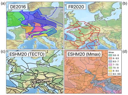
Figure 5 Large-scale area source zonations (LASZs) assumed for DE2016 (a) and FR2020 (b) and the two LASZs for ESHM20 based on regional tectonics (c) and maximum magnitude (d). Colours for DE2016 indicate the groupings of LASZs (from Model A) sharing a common b value.

DE2016 follows the methodology set out by Stromeyer and Grünthal (2015), who describe the uncertainty in cumulative activity rate ν at each magnitude m from the covariance matrix such that

$$\begin{array}{}\text{(2)}& \begin{array}{rl}{\mathit{\sigma }}^{\mathrm{2}}\left(m\right)& ={\left(\genfrac{}{}{0ex}{}{\mathrm{1}}{-m}\right)}^T\mathbf{COV}\left(a,b\right)\left(\genfrac{}{}{0ex}{}{\mathrm{1}}{-m}\right)\\ & ={\mathit{\sigma }}_a^{\mathrm{2}}-\mathrm{2}m{\mathit{\sigma }}_a{\mathit{\sigma }}_b+m^{\mathrm{2}}{\mathit{\sigma }}_b^{\mathrm{2}}.\end{array}\end{array}$$

The cumulative rate of events greater than or equal to magnitude ν_c(m) then becomes

$$\begin{array}{}\text{(3)}& {\mathit{\nu }}_{\mathrm{c},i}\left(m\right)={\int }_M^{M_{\mathrm{MAX}}}{\mathrm{10}}^{\stackrel{\mathrm{‾}}{a}-\stackrel{\mathrm{‾}}{b}m+\mathit{\sigma }\left(m\right)z_i}dm,\end{array}$$

where z_i is the number of standard deviations of a standard normal distribution. The incremental activity rate in any given bin of width dm then simply becomes ${\mathrm{10}}^{\stackrel{\mathrm{‾}}{a}-\stackrel{\mathrm{‾}}{b}m+\mathit{\sigma }\left(m\right)z_i}$. The uncertainty in each magnitude is now represented by a marginal distribution of 𝒩(0, σ(m)). This epistemic uncertainty can thus be mapped onto a discrete set of $i=\mathrm{1},\mathrm{2},\mathrm{\dots },k$ branches such that z_i and its corresponding weight, w_i, are discrete approximations to the standard normal distribution according to the Gaussian quadrature approach of Miller and Rice (1983). As Eq. (1) is dependent on M_MAX, the posterior distribution f(M_MAX) returned by the EPRI approach for each zone is first approximated into five discrete branches using the same Gaussian quadrature method. Each of the five M_MAX values is then input into Eq. (3), which is then discretised into four branches to approximate 𝒩(0, σ(m)). The epistemic uncertainty in the MFR for each area source is therefore represented by 20 logic tree branches (shown in Fig. 2).

ESHM20 starts from a similar point to DE2016, as it defines $\widehat{a}$, $\widehat{b}$, and COV(a,b) according to Stromeyer and Grünthal (2015) but then approximates the distribution differently. Monte Carlo sampling is used to generate 1 million realisations of a and b from the multivariate normal distribution, and from these samples the pairs corresponding to the 16th, 50th, and 84th percentile values are taken to define the lower, middle, and upper branches respectively, with weights of 0.2, 0.6, and 0.2 respectively. M_MAX is defined independently of a and b using the three branches described previously. Though ESHM20 evaluates the multivariate distribution of a, b, and COV(a,b) in a slightly less formally correct manner compared to DE2016, one would still expect the distribution of resulting hazard curves to be similar. However, ESHM20 diverges further from both the DE2016 and the FR2020 approaches by introducing as an alternative set of MFR branches a tapered Gutenberg–Richter recurrence model (Kagan, 2002):

$$\begin{array}{}\text{(4)}& \mathit{\nu }\left(M_{\mathrm{0}}\right)={\left({\displaystyle \frac{M_{\mathrm{t}}}{M_{\mathrm{0}}}}\right)}^{\mathit{\beta }}\exp \left({\displaystyle \frac{M_{\mathrm{t}}-M_{\mathrm{0}}}{M_{\mathrm{cm}}}}\right)\text{for}{M}_{\mathrm{t}}\le M_{\mathrm{0}}<\mathrm{\infty },\end{array}$$

where M₀ is the seismic moment of an event with magnitude m, M_t is the threshold moment, β=bln (10), and M_cm is the corner moment. Unlike the truncated Gutenberg–Richter model, the tapered Gutenberg–Richter distribution is theoretically unbounded at large moments; however, the exponential decay in the functional form above M_cm effectively tapers the rate of events to triviality for magnitudes larger than the corresponding M_cm, so truncation can be safely applied within 0.2–0.3 magnitude units above M_cm with only minimal impact on the hazard calculation. For the set of branches corresponding to this distribution, the rate and b value are fixed according to the $\widehat{a}$ and $\widehat{b}$ values defined previously, while the three M_MAX branches are applied as epistemic uncertainty in M_cm. In total, for area sources the source model logic tree contains 12 branches to represent the uncertainty in the MFR: for the truncated Gutenberg–Richter model three branches of a and b and another three of M_MAX and for the tapered Gutenberg–Richter model only three branches for M_cm.

For both DE2016 and ESHM20 it is also necessary to define activity rates for both the smoothed seismicity sources and the active fault sources. Because of its implicitly non-parametric approach to defining activity rates, no MFR uncertainty is considered for the zoneless smoothed seismicity model of DE2016. Similarly, for ESHM20 the smoothed seismicity model is optimised through an iterative forecast testing approach, which yields a single preferred smoothed seismicity model without epistemic uncertainty in the MFR. Both models do define epistemic uncertainty in the activity rates for the fault-based models. In the case of DE2016 the maximum magnitudes on the composite fault sources are characterised according to their fault dimension using a normal distribution of 𝒩(M_MAX,0.3) (Vanneste et al., 2013). These distributions are mapped onto five branches using the Miller and Rice (1983) methodology. On-fault recurrence is modelled using a truncated Gutenberg–Richter relation, but as the authors could not constrain the proportion of aseismic slip, they opted to assign the seismicity for M_W≥5.3 to the fault sources and the rest to their respective catchment zone (Model C, zones C15 and C22), with the proportion of seismicity rate for each fault assigned according to the relative length of the fault. This results in a total of 20 MFR branches on the fault sources, comprising five M_MAX branches and the four branches of recurrence uncertainty from the catchment zones. In ESHM20 the recurrence models for the active fault sources also use a truncated Gutenberg–Richter model, albeit moment balanced from the geological coseismic slip rate. As the slip rates are themselves uncertain, three branches for alternative coseismic slip rates are considered along with three branches for M_MAX.

FR2020 takes a different approach to characterising epistemic uncertainty compared to either ESHM20 or DE2016. For each area source and for each larger-scale superzone the seismicity is represented by a truncated Gutenberg–Richter model represented by $\widehat{a}$, $\widehat{b}$, and C(a,b), in addition to the posterior density function f(M_MAX) that is defined for each superzone. Rather than discretise the distributions of ν(m) (as DE2016) or of a, b, and M_MAX into a small set of branches according to Miller and Rice (1983), Drouet et al. (2020) instead use Monte Carlo sampling, drawing 100 samples from each distribution, with each sample then represented as an equally weighted MFR branch (weight $=\mathrm{1}/\mathrm{100}$) in the logic tree. Samples are drawn independently from f(M_MAX) and the multivariate normal distribution representing the a and b value $\mathrm{MVN}\left(\begin{array}{c}\widehat{a}\\ \widehat{b}\end{array},\mathbf{C}\left(a,b\right)\right)$. This results in a total of 400 source model branches from four source models (GTR, EDF, IRSN, and zoneless), each with 100 MFR samples. Implementation of the model revealed that the original authors had adopted a stratified sampling strategy for a and b, which is illustrated in more detail in the Supplement Part A Sect. S2.

2.3 Upper Rhine Graben source example: similar approaches, different outcomes

To illustrate how the different approaches to characterisation and implementation of the MFRs in a logic tree can yield quite different distributions of activity rates for a given source, even where many inputs to the source model are similar, we consider the case of the Upper Rhine Graben (URG). Among the different source zonations within the different logic trees there are some differences to the exact shape of the source(s) in the Upper Rhine, though most models describe a source that follows the main outline of the graben starting just north of the Basel earthquake sequence in the south and terminating close to Karlsruhe in the northwest. We select the DEAS107 zone from the ESHM20 unified area source model branch, the Fosse-Rhenan Sud (FRS) zone from the FR2020 GTR source zonation, and the D051 zone from the DE2016 model to look at in detail as they depict similar geometries with respect to the spatial seismicity distribution. These sources are shown with seismicity from their respective earthquake catalogues in the top row of Fig. 6. Here we observe a first point of divergence, as the catalogues show remarkably different patterns of seismicity for the same zone. This is somewhat surprising as ESHM20 adopts the same earthquake catalogue as FR2020 within the French territory, namely FCAT-17 (Manchuel et al., 2018), and the same catalogue within the German territory as DE2016 for the post-1900 seismicity. Differences emerge in the pre-1900 earthquake catalogues as ESHM20 adopts the European Preinstrumental Earthquake Catalogue (EPICA) (Rovida et al., 2022), which is compiled independently from the other catalogues.

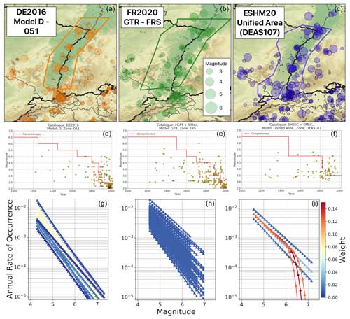
Figure 6 Example comparison of fit and representation of earthquake recurrence for the Upper Rhine Graben (URG) for DE2016 (a, d, g), FR2020 (b, e, h), and ESHM20 (c, f, i). Example geometry of the selected URG seismic source in different models and the respective earthquake catalogues with symbols scaled according to magnitude (a, b, c), distribution magnitude with time for the respective zones and the corresponding temporal completeness magnitude assumed by the model (d, e, f), and distribution of magnitude frequency relations for the zone colour scaled according to weight. All catalogues share the same symbol size scaling with magnitude (a, b, c), and all magnitude frequency distributions share the same colour scale (g, h, i).

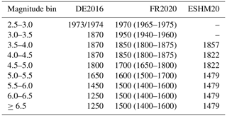
The next point of divergence can be seen in the estimate of completeness magnitude and its variation in time, which can be seen in the middle row of Fig. 6 and is given in Table 2. FR2020 and DE2016 estimate completeness using the method of Hakimhashemi and Grünthal (2012), although adopting different spatial zones to apply the method, while ESHM20 estimates completeness using an inversion method based on forecast testing (Nandan et al., 2022). Drouet et al. (2020) provide the uncertainty range for the completeness estimates, and although the preferred values are different for many magnitude bins, the earliest years of completeness for magnitudes in the range $\mathrm{4.0}\le M_{\mathrm{W}}\le \mathrm{6.5}$ for the DE2016 and ESHM20 models are consistent with the uncertainty range shown in Table 2 for FR2020. Taking the best estimates, however, and contrasting these against the catalogues (shown in the middle row of Fig. 6), it is obvious that both the catalogues and the completeness estimates are dissimilar.

The bottom row of Fig. 6 shows the distributions of activity rate with magnitude for all the MFR branches assumed by the respective logic trees. Although each model uses some form of maximum likelihood estimate (Johnston et al., 1994; Stromeyer and Grünthal, 2015) to determine the Gutenberg–Richter parameters for the zone, the results are significantly different. ESHM20 has an expected a and b value of 1.9565 and 0.7334 respectively, which are mapped onto three branches of a−b pairs: (1.886, 0.685), (1.9565, 0.7443), and (2.0278, 0.803). By contrast, FR2020 yields a and b values of 2.3711±0.182 and 0.8696±0.0918 respectively, with ρ_ab=0.8991, and while DE2016 is dependent on M_MAX, the a and b values range from 3.89 to 2.86 and from 1.08 to 0.95 respectively. Not only do the MFR parameters themselves then vary significantly, but the different mappings onto logic tree branches also yield significantly different activity rate distributions, as illustrated in Fig. 6. ESHM20 places more weight on the middle branches, and in this case the MFR logic tree mixes both the truncated Gutenberg–Richter distribution and the tapered Pareto distribution. FR2020 clearly shows the largest spread of MFRs, which arises in part from the independence of a and b from M_MAX and in part because of the large number of evenly weighted sample values. DE2016 is something of a middle point, with a narrower range of values and notably higher weights on a specific subset of branches.

Table 2 Variation in completeness window for each magnitude bin assumed for the selected URG source zone.

The comparison here is not an exhaustive description of all the reasons for the differences in seismic hazard that we will eventually see between the three models, but it is illustrative of how they can diverge significantly in the critical information for PSHA (namely activity rate per magnitude bin) despite adopting theoretically similar approaches. Particularly insightful is the contrast in the way in which the distribution of a and b is mapped onto the epistemic uncertainty, which would potentially suggest that even if the three models produced a similar fit in their recurrence models, they could still diverge significantly in the resulting activity rate distributions inside the PSHA calculation. We discuss in the “Discussion and conclusion” section the implications for future harmonisation of the seismic hazard, but a key point to take from this brief analysis is that each step of the process, from the basic earthquake data through to the distribution of activity rates, requires both transparency and scrutiny. Though the models considered here are arguably better documented than many, there are still many steps in the processes that are not completely described, or if they are described it may be difficult to perceive how this can influence the hazard. These factors contribute to the differences in hazard model components and hazard model outputs shown in Sects. 4 and 5.

2.4 Ground motion models

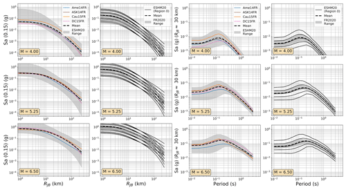
For the ground motion model (GMM) logic tree it is not necessarily the technical process itself and the decisions made therein that differ significantly between the three PSHA models but rather the general philosophy of how to characterise epistemic uncertainty. Specifically, between the three models we see an example of a multi-model (or “weight-on-model”) GMM logic tree (FR2020), a hybrid multi-model logic tree with backbone scaling factors (DE2016), and a fully regionalised scaled-backbone logic tree (ESHM20). All three models explicitly invoke the same objective of “capturing epistemic uncertainty in terms of the centre, body and range of the technically defensible interpretations of available data” (U. S. Nuclear Regulatory Commission, 2012). To contrast distributions of GMMs from different PSHA models, we created a set of trellis plots in which the GMM selections from two different models are plotted side by side for the same set of predictor variables. The range of GMM median or standard deviation values for the contrasting model is described by a shaded region beneath the GMMs for the model in question.

The GMM logic tree for DE2016 was initially based on a multi-model approach, with five models identified as suitable for application in Germany (Akkar et al., 2014a; Bindi et al., 2014; Derras et al., 2014; Cauzzi et al., 2015; Bindi et al., 2017), but it adds to each of these models a set of scaling factors to the median ground motions (0.7, 1.0, 1.25, and 1.5) to account for epistemic uncertainty in regional stress drop. Of the five models selected, Akkar et al. (2014a), Bindi et al. (2014), and Derras et al. (2014) are fit to data from the pan-European RESORCE dataset, while Cauzzi et al. (2015) and Bindi et al. (2017) are fit using data predominantly from Japan (supplemented by some records from other regions of the globe). The latter is fit using records from the NGA-West2 dataset but using a simpler functional form than the NGA-West2 GMMs. This makes Bindi et al. (2017) better suited for the level of parameterisation commonly found in moderate- to low-seismicity regions where seismogenic sources are predominantly based on distributed seismicity rather than directly on active faults. The DE2016 GMM logic tree combines a standard multi-model approach with elements of a scaled-backbone approach to capture some of the uncertainty in the underlying seismological properties of the target region; hence, we refer to it as a hybrid multi-model and backbone GMM logic tree.

Grünthal et al. (2018) outline several key factors that influence their decision-making process: (i) varying strengths of the different databases of ground motion, e.g. tectonic similarity for Europe (RESORCE), a wealth of short-distance records (NGA-West2), and detailed site parameterisation (Japan – Cauzzi et al., 2014); (ii) variation in functional form and how this influences ground motion prediction for small- to moderate-magnitude events; and (iii) the observation of several earthquakes with higher-than-average stress drop in stable regions of France, Germany, and the UK. The multi-model approach and the choice of models selected largely address the first two of these issues. Three different datasets (RESORCE, NGA-West2, and Japan) are represented, which also implicitly incorporate GMM source-region-to-source-region variability (i.e. Europe, western United States, and Japan). The highest weight assigned to the three GMMs derived from RESORCE and then split evenly between the three models therein is 0.5, while the Cauzzi et al. (2015) and Bindi et al. (2017) models receive equal weights of 0.25. Functional form variation and parameterisation are accounted for by mixing classical random effect models (each with slight differences in functional form) with purely data-driven neural network models (Derras et al., 2014).

The GMM logic tree adopted for FR2020 is the simplest of the three, using four ground motion models each assigned an equal weight of 0.25 (Ameri, 2014¹; Abrahamson et al., 2014; Cauzzi et al., 2015, with variable reference V_S30; Drouet and Cotton, 2015, using rupture distance and with 10 MPa stress drop for large-magnitude events). Two of these models (Ameri, 2014; Drouet and Cotton, 2015) are based exclusively on French seismological data, while the Abrahamson et al. (2014) model is fit to records from the NGA-West2 dataset (global in scope but with most records originating from California), and the Cauzzi et al. (2015) model is fit predominantly to Japanese strong-motion data. None of the selected GMMs is based on the pan-European RESORCE ground motion dataset (Akkar et al., 2014b), although Drouet et al. (2020) indicate that several of the GMMs that were derived using pan-European ground motion data were considered in the selection process. The analysis to support their model selection is based on the exploration of the model space of the GMMs using Sammon's maps (Scherbaum et al., 2010), which reveal that the four models are relatively well separated within the model space described by all pre-selected GMMs and by a set of reference models derived from the mean of the considered GMMs scaled up and down (representing stress drop variation) and with faster or slower attenuation. In this sense, the multi-model logic tree accounts for epistemic uncertainty in both the model functional form and the geophysical properties of the target region, with the latter being represented by the different GMM source regions implicit within the selected models: France (Ameri, 2014; Drouet and Cotton, 2015), the western United states (Abrahamson et al., 2014), and Japan (Cauzzi et al., 2015).

In practice, the DE2016 and FR2020 approaches yield similar outcomes, with the same three source regions represented: local/Europe, Japan, and the western United States, with the local region receiving a weight of 0.5 and the other two a weight of 0.25 each. The two sets of GMMs for the DE2016 and FR2020 models are compared in terms of their range of median ground motions (Fig. 7) and their aleatory uncertainty σ_T (Fig. 8). For these comparisons and those in the subsequent figures (Figs. 9 to 12), the three scenario magnitudes (M_W4.0, 5.5 , and 6.5) are chosen because they represent the minimum magnitude considered by the models (M_W4.0), the typical controlling magnitude of the hazard for return periods of engineering interest (M_W5.5), and a feasible but low-probability extreme scenario (M_W6.5) that is close to the M_MAX in stable zones but lower than the M_MAX of the active fault sources found in the Rhine Graben and Alpine front.

The uncertainty in stress drop is the motivation behind adding the additional scaling factors, which capture both the possibility that stress drop may be lower in Germany than in the respective source regions of the models (0.75) and the possibility that it is higher (1.25 and 1.5). Weights of 0.36 are assigned to each of the 1.0 and 1.25 scaling factors, while the outer branches (for lower-than-average or much-higher-than-average stress drop) are assigned smaller weights of 0.14 each. This pushes the balance of the weight toward higher stress drop in Germany.

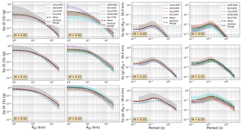
Figure 7 Trellis plots comparing the median ground motions of the GMM selections of the FR2020 and DE2016 logic trees. (left) Attenuation with distance for Sa (0.15 s) for M_W 4.0, 5.25, and 6.0 and (right) scaling with period at a site R_JB 30 km from the source for M_W 4.0, 5.25, and 6.0. The range of values from the compared models is shown by the grey-shaded region in each plot, while the dashed black lines show the sum of the median ground motions from each model (μ_i) weighted by their logic tree weights (w_i): ${\sum }_i({\mathit{\mu }}_i\cdot w_i)$.

Compared to the strategies adopted for FR2020 and DE2016, the ESHM20 model has taken a different approach to defining a GMM logic tree that captures the centre, body, and range of the technically defensible interpretations of available data, and it does so by abandoning the multi-model concept entirely in favour of a regionalised scaled-backbone logic tree. The full explanation of the logic tree, including both its motivation and its calibration, is given in Weatherill et al. (2020). This change in approach is motivated in large part by the development of the Engineering Strong Motion (ESM) database and flatfile (Lanzano et al., 2019), which increases the number of ground motion records available in Europe by nearly an order of magnitude, particularly those of small- to moderate-magnitude earthquakes, including many more from France and Switzerland compared to RESORCE. The backbone GMM is fit to this dataset (Kotha et al., 2020), but with such a large volume of data additional random effects are included to capture region-to-region variability in the stress parameter scaling of the model (δL2L_l) and in the attenuation (δc₃, where c₃ is the coefficient of the anelastic attenuation term of the model). These two random effects are both normally distributed variables with means of 0 and standard deviations of τ_L2L and ${\mathit{\tau }}_{c_{\mathrm{3}}}$ respectively, and individually they quantify the total regional variability in the stress parameter and residual attenuation within Europe. For regions with little or no ground motion data, the distributions of 𝒩(0, τ_L2L) and $\mathcal{N}(\mathrm{0},{\mathit{\tau }}_{c_{\mathrm{3}}})$ are mapped onto sets of discrete branches using the method of Miller and Rice (1983), making the model a scaled-backbone model. Where data are available the distributions can be adjusted to reflect the local stress parameter or attenuation properties implied by the data; thus the model is also regionalisable.

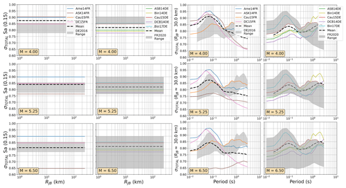
Figure 8 As Fig. 7 but comparing the aleatory uncertainty distributions of the FR2020 and DE2016 GMM logic trees. The dashed black lines refer to the sum of the aleatory variabilities of each GMM (σ_i) weighted by their logic tree weight (w_i): ${\sum }_i({\mathit{\sigma }}_i\cdot w_i)$.

Even in the larger ESM flatfile there are few events from Germany, and those that are present are almost all located in the Upper Rhine Graben and Alpine Foreland. In France the majority of earthquake and records come from the Alpine and Pyrenees regions. Observations were available for the regions where δc₃ could be calibrated, so regions of similar δc₃ were grouped together to differentiate between regions of slower, average, or faster attenuation. These differences are reflected in the model, where the attenuation parameters of the backbone GMM for sites in these regions are adjusted to incorporate these differences. Altogether, the regionalised scaled-backbone logic tree maps the unadjusted (un-regionalised) δL2L_l term onto five branches and the regionalised δc₃ term onto three branches, resulting in 15 GMM branches altogether. The median accelerations predicted by ESHM20 GMMs are compared against those of FR2020 and DE2016 in Figs. 9 and 10 respectively and the aleatory uncertainties in Figs. 11 and 12.

Figure 9 As Fig. 7 but comparing the median ground motions of the ESHM20 and FR2020 GMM logic trees.

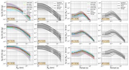
Figure 10 As Fig. 7 but comparing the median ground motions of the ESHM20 and DE2016 GMM logic trees.

Among the most important trends to be seen in the plots in Figs. 7 to 12 are the general tendencies toward higher median ground motions at short distances and small magnitudes for the GMM logic trees of the DE2016 and ESHM20 models compared to those of FR2020. For larger magnitudes the trends reverse, and it is the ESHM20 GMM logic tree that provides a lower central tendency in the ground motions. At intermediate magnitudes and distances, where we are best constrained by data, ESHM20's GMM logic tree tends toward lower short-period motions at most magnitudes and distances, while longer-period motions are comparable. However, we note that the very high and very low stress parameter branches of the ESHM20 GMM logic tree that envelope the range of values in the plots have very little weight associated with them, and it is the three more central branches that have the greatest influence on the mean hazard.

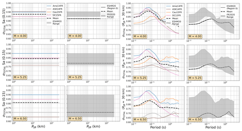
Figure 11 As Fig. 8 but comparing the aleatory uncertainty distributions of the FR2020 and ESHM2020 GMM logic trees.

For the DE2016 and FR2020 comparisons, the DE2016 GMMs tend to skew higher. This reflects the influence of the stress drop scaling, where more weight is put on toward the scaling factors greater than or equal to 1.0. Without these adjustments the GMM selections would likely have returned a similar centre and range of ground motions, except at near-source distances (R_JB<10 km) where the Derras et al. (2014) GMM with the point-source to finite rupture distance correction seems to extrapolate toward much higher motion than the other models.

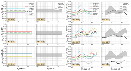
Figure 12 As Fig. 8 but comparing the aleatory uncertainty distributions of the ESHM2020 and DE2016 GMM logic trees.

For the aleatory variability the ESHM20 is based on a scaled-backbone model with no branches for epistemic uncertainty in this term; thus the range of σ_T collapses to a simple line in Figs. 11 and 12. What is evident, however, is the heteroscedastic variability that is present in the ESHM20 model and in the Abrahamson et al. (2014) model. This results in lower σ_T at high magnitudes, which in turn lowers the aleatory uncertainty in the ESHM20 model compared to the other GMM logic trees. We also observed that the ESHM20 model shows a lower aleatory variability in general compared to the spread found in other GMM logic trees. Two factors play a role here: the first is that the Kotha et al. (2020) model was derived using robust linear mixed-effect regression that down-weights outlier values and the second is that the ESHM20 GMM implementation adopts different site-to-site variability (ϕ_S2S) for the cases when the site condition (V_S30) is measured and when it is inferred from a proxy (Danciu et al., 2021; Crowley et al., 2021). For the measured V_S30 case, which is the one being considered in the ESHM20 application, ϕ_S2S is reduced compared to most other GMMs shown here because it is fit to the site-to-site variability of the subset of stations with measured V_S30, while most other models have calibrated this variability based on records from stations that mix measured and inferred V_S30.

3 Harmonising model implementations into a common software format

We have so far looked at some of the fundamental differences in the seismic hazard inputs between the three national seismic hazard models, and though there are different approaches and philosophies underpinning each, there are also many key similarities, most notably in the types of sources being adopted (i.e. uniform area zones; smoothed seismicity; and, in the case of ESHM20 and DE2016, active fault surfaces). An important difference, however, is not just in the construction of the inputs but also in how they are processed in the PSHA calculation. Here, the PSHA calculation software plays an important role. Each of the three models was implemented in a different PSHA software: FR2020 used a proprietary software developed by Fugro that is based on a customised version of FRISK88 (McGuire, 1976); DE2016 also used a proprietary software that is their own customisation of FRISK88 for the area and fault sources, which was combined with their own software code to implement smoothed seismicity PSHA; and ESHM20 was developed using OpenQuake (Pagani et al., 2014).

Our first major objective in this work was to harmonise all three models into a common format around the OpenQuake engine seismic hazard and risk software. This harmonisation serves multiple purposes. The first is to migrate the models from the proprietary software in which they were originally implemented and to support them using open-source software so that they can be reproduced by other parties. The second purpose is the main objective of this paper, which is to define a common representation of hazard inputs and outputs that will allow for the quantitative comparisons shown in Sects. 4 and 5. Finally, OpenQuake includes both a seismic hazard calculator and a seismic risk calculator, which in combination with the exposure and vulnerability models provided as part of ESRM20 allow us to explore implications of the different models in terms of seismic risk. This latter objective will, however, be the subject of a future study and is beyond the scope of the current paper.

3.1 PSHA software comparisons: rationale and applications

Although PSHA models have developed in sophistication over the decades, the fundamental framework for PSHA has remained largely unchanged since its establishment by Cornell (1968) and McGuire (1976). Arguably the most notable evolutions in practice emerge with the “grand inversion” methodology for modelling fault systems (e.g. Field et al., 2015, 2024) and more widespread usage of Monte Carlo techniques (e.g. Ebel and Kafka, 1999; Musson, 2000; Weatherill and Burton, 2010; Assatourians and Atkinson, 2014). These later adaptations do not alter this core probabilistic framework but rather evaluate it in a manner that may be flexible or better suited to incorporating new modelling developments or providing input into a broader range of applications. Yet, despite the robustness of the conceptual probabilistic seismic hazard integral, different PSHA software can be remarkably divergent in the way the input source and ground motion models are processed and translated into the PSHA framework.

Differences between PSHA software can be broadly grouped into three categories:

• Irreconcilable discrepancies owing to fundamental differences in software operation. These can include characterisation of the seismic source and/or magnitude frequency relation and their discretisations within the hazard integral; treatment of rupture finiteness in distributed seismicity sources; and its scaling with earthquake magnitude, calculation of fault rupture to site distances, and evaluation and/or approximation of the statistical density functions to retrieve probabilities of exceedance of ground motion. Such differences can be identified but not necessarily replicated from one software to another without significant changes to the code.

• Implementation discrepancies, which mainly refer to bugs or errors in the source codes themselves, potential instability due to rounding errors, or different interpretations of ambiguously described features or parameters in implemented models such as GMMs. These can be identified and resolved by following quality assurance procedures and can be greatly assisted by model authors providing open-source implementations of their models.

• Free modelling parameters and configuration choices that allow users to control the operation of the software but that are seldom fully documented (particularly in scientific papers). These may resemble the irreconcilable discrepancies more if one software implements a part of the hazard calculation in a flexible manner that affords the user control of the operation, while another software may hard-code this same process and afford the user no control.

The way that different software packages characterise common elements of a PSHA calculation and the corresponding impacts on the resulting hazard curves have been evaluated as part of the PEER Probabilistic Seismic Hazard Code Verifications (PEER Tests hereafter) (Thomas et al., 2010; Hale et al., 2018). These are elemental PSHA calculations usually comprising a single source, a ground motion model, and a limited number of target sites with fixed properties, which are designed specifically to assess how the different software programmes approach a particular modelling issue. The results are compared against either “exact” solutions calculated by hand, where possible, or the range of curves determined from the participating PSHA codes when the problem cannot be evaluated by hand.

The PEER Tests have been particularly insightful in identifying how and why PSHA codes diverge, which is especially important given that many codes participated in them (both proprietary and open source) that are widely used in commercial application. As they are elemental in nature, however, they cannot necessarily predict the extent to which different codes will yield different outputs for seismic hazard at a given location, where many modelling differences come into play. The importance of this type of application and the benefits of multi-software implementations of a seismic hazard model as part of a quality assurance (QA) process for the design of critical facilities have been emphasised by Bommer et al. (2015) and Tromans et al. (2019), among others, and both are becoming more widely used in practice. The QA application is only one context, however, and arguably a favourable one in which multiple parties are involved, and resources are often made available to document and debate the implementations and to resolve discrepancies as and when they emerge.

More relevant for the case at hand is migration of an existing or established hazard model from one software to another. Here the challenges are different, as the existing model forms the reference, and the new software may need to replicate the behaviour of the previous one in order to ensure consistency in the outputs. In some cases, if the new software user is different from or does not have the support of the original software developer, and the source code of the software is closed, then there can often be critical elements of the PSHA calculation process that are hidden from the user. In this instance complete agreement between the existing and migrated models may not be possible, primarily due to the irreconcilable differences between the software highlighted above. Instead, a target level of “acceptable agreement” between the previous and new implementation needs to be defined (e.g. Abbot et al., 2020; Allen et al., 2020).

In the migration processes described in this section, we set a target level of agreement in terms of the OpenQuake-calculated seismic hazard curves at given target sites agreeing with those produced from the original PSHA software code to within a ±10 % annual probability of exceedance (APoE) for the corresponding range of ground motion intensity measure levels (IMLs) for APoEs greater than 10⁻⁴ (corresponding to a return period of approximately 10 000 years). Although in many cases agreement can be achieved for lower APoEs, the irreconcilable differences due to issues of discretisation, rounding, numerical instability etc. may begin to influence the extreme tails of the distributions that assume greater importance at these longer return periods. An APoE of 10⁻⁴ is sufficient to span the range of return periods considered for conventional design building codes, which reflect the applications for which these specific hazard models are intended. As both the FR2020 model and the DE2016 model have logic trees, we undertake comparisons in two steps, the first comparing specific branches of the logic tree to ensure broad agreement over source and ground motion model combinations and the second comparing the curves in terms of the respective means and quantiles. We note that from the seismic hazard curves similar agreement targets could be set in terms of the IMLs for a fixed range of APoEs, which may be slightly more intuitive. Both options were explored, and no cases were found in which the agreement in curves for the IMLs failed to reach the set ±10 % target when the agreement in terms of APoEs did. As all three software programmes considered return seismic hazard curves in terms of PoE for a user-input set of IMLs, and statistics of means and quantiles were calculated based on PoE, we opted to use APoE as the variable for the comparisons to avoid introducing potential discrepancies from different interpolation approaches. Summaries of the migration issues for both FR2020 and DE2016 can be found in the Supplement Part A Sects. S3, S4, and S5, and further details of the issues encountered in the migration of FR2020 to OpenQuake can be found in Weatherill et al. (2022). Illustrative comparison plots of the two software implementations for both national seismic hazard maps and seismic hazard curves at selected locations can be seen in the Supplement Part B.

3.2 Defining means and quantiles

In OpenQuake the mean is calculated as the weighted arithmetic mean of the probabilities of exceedance (PoEs) for each given intensity measure level (IML). Similarly, quantiles are determined based on the probabilities of exceedance for each intensity measure level by sorting the PoEs from the lowest to the highest at each IML and interpolating the corresponding cumulative density function to the desired quantile values (typically 0.05, 0.16, 0.5 (median), 0.84, and 0.95). As OpenQuake adopts the earthquake rupture forecast (ERF) formulation for the PSHA calculation (Field et al., 2003), all hazard statistics are extracted from the probabilities of exceedance rather than the rates of exceedance. This formulation of the mean and quantiles represents one of several different ways of retrieving this term. Other PSHA software programmes may apply the statistics to the IMLs for a given PoE and/or work with the geometric means rather than arithmetic means, and each approach yields different results. From communication with the model developers, we verified that FR2020 defines the mean hazard as the arithmetic mean of the probabilities of exceedance, while for DE2016 the means are based on the arithmetic mean of the annual rates of exceedance. For consistency with OpenQuake, in the comparisons of means and quantiles, we retrieved these values from the complete suite of hazard curves and processed them identically rather than taking the mean or quantiles from the software itself.

3.3 Source-to-source correlation in MFR epistemic uncertainties

We see in Sect. 2 how the three different models attempt to translate the uncertainty in a, b, and COV(a,b) into the logic tree and how this yields quite different distributions of activity rates. A factor that is not discussed is the issue of source-to-source correlation in the MFRs. To summarise, consider an idealised model with just four area sources, each with their own truncated Gutenberg–Richter MFR, and a corresponding logic tree with three branches for uncertainty in a and b (e.g. $-\mathrm{\Delta }\cdot \left(a,b\right),\left(\stackrel{\mathrm{‾}}{a,b}\right),+\mathrm{\Delta }\cdot \left(a,b\right))$ and three for uncertainty in M_MAX (e.g. $M_{\mathrm{MAX}}^{\mathrm{LOW}},\stackrel{\mathrm{‾}}{M_{\mathrm{MAX}}}+M_{\mathrm{MAX}}^{\mathrm{HIGH}}$). If the MFRs are fit independently for each zone, then the resulting logic tree would need to permute every combination of the MFR parameters for each source, which would in this simple case result in 9⁴=6561 logic tree end branches, i.e. ${\left(N_{\mathrm{BRANCHES}}\right)}^{N_{\mathrm{SRCS}}}$. Applying this same logic to the area source zonations for DE2016, for example, we have between 31 and 107 sources per model and 20 MFR branches, which would result in between 20³¹ and 20¹⁰⁷ logic tree branches for each source model. This is clearly intractable for any PSHA calculation software, and OpenQuake cannot even construct such a logic tree from which to sample. A common alternative is to assume perfect correlation between the sources, which in the idealised case would be to apply the same branches (e.g. $-\left(a,b\right)|M_{\mathrm{MAX}}^{\mathrm{low}},\left(\stackrel{\mathrm{‾}}{a,b}\right)|M_{\mathrm{MAX}}^{\mathrm{LOW}},+\left(a,b\right)|M_{\mathrm{MAX}}^{\mathrm{LOW}},-\left(a,b\right)|$ $\stackrel{\mathrm{‾}}{M_{\mathrm{MAX}}},\mathrm{\dots },+(a,b)|M_{\mathrm{MAX}}^{\mathrm{HIGH}}$) to all of the sources at the same time. This results in a more manageable logic tree of just 9 branches in the simple idealised case and 20 MFR branches per source model in the DE2016 case.

Both DE2016 and ESHM20 adopt discrete MFRs for each of the sources, meaning that in order to execute the calculation, perfect correlation between sources had to be assumed in both cases. However, by sampling the MFRs for each source separately in the 100 branches, FR2020 preserves independence in the source model MFRs. This issue of correlation can impact on the outcomes of the hazard as the assumption of perfect source-to-source correlation in MFRs could conceivably assign disproportionately large weights to the extreme cases such that all sources may have higher or lower activity rates. This inflates the uncertainty, meaning that the resulting hazard distributions may be larger than intended, potentially skewing the mean toward higher values compared to the case in which MFR epistemic uncertainties are characterised independently for each source. Work is currently ongoing to explore this issue and its impacts on seismic risk assessment for a country in further detail.

3.4 Calculation scale

A final issue of PSHA implementation relates to the scale of calculation, by which we refer to the volume of data and, by extension, the CPU time and RAM needed to execute the PSHA for logic trees of this size. Each of the three software programmes address this differently, and as two of the software programmes are proprietary, we have not been able to benchmark the calculations. For OpenQuake, however, this type of logic tree with many source and MFR branches has not been efficiently handled at the time of writing. The main reason for this is that for each source model and MFR branch a new earthquake rupture forecast is constructed. This requires re-calculation of distances and ground motions for each logic tree branch and MFR branch, increasing both the CPU requirements and the RAM requirements. Calculations here were run on a 192 CPU server with 760 GB RAM, and this was insufficient to execute the calculations in a single run. Instead, the models for FR2020 and DE2016 were split into subsets of branches, and the resulting hazard curves were later recombined and post-processed to retrieve the mean and quantiles. It is hoped that future efforts will be undertaken to improve the efficiency of the calculations for this type of epistemic uncertainty, which is commonly applied in regions of low to moderate seismicity.

4 Quantitative comparisons of the seismogenic source models by visualising activity rate model space

In Sect. 2 we show the overall structure of the different models, contrasting some of the assumptions behind them and looking in detail at the France–Germany border region to understand the differences in catalogues, definitions of source models, and the fitting and characterisation of the recurrence models. Although this process brings to light some of the main factors that go toward explaining the differences in seismic hazard results shown in the next section, it is also important to be able to quantify and interpret differences in the two primary components of the PSHA model: the seismic source model and the ground motion model. Comparisons at this point can be particularly useful as they can allow us to understand the cumulative impact of the diverging steps that have led to the construction of the respective source and ground motion models before these are then integrated into the PSHA calculation. A crucial motivation for the migration of the PSHA models into a common software, as described in detail in Sect. 3, is to have the three models represented in a common format that allows us to isolate the model-to-model differences from the software differences. In this section all the analyses work with the OpenQuake implementations of the models rather than the original implementations (in the case of FR2020 and DE2016).

4.1 Interpreting the seismogenic source model space using descriptive statistics

Section 2 explains how all three models share some similarities in the source types that they use, as well as their differences. As each model adopts a logic tree with epistemic uncertainty in both the source types and the recurrences, how can one quantitatively compare not just the sources but also their respective distributions? The starting point is to render each source into a common representation that allows for quantitative comparisons of the models and their respective distributions. Each source branch of each model is translated into a three-dimensional array $\mathit{\lambda }(\mathit{\varphi },\mathit{\theta },\mathit{M})$ of longitude, latitude, and magnitude, with each cell containing the incremental rate of activity for the corresponding longitude, latitude and magnitude bin λ_ijm, where $i=\mathrm{1},\mathrm{2},\mathrm{\dots },N_{\mathit{\varphi }}$ corresponds to the longitude bin, $j=\mathrm{1},\mathrm{2},\mathrm{\dots },N_{\mathit{\theta }}$ to the latitude bin, and $m=\mathrm{1},\mathrm{2},\mathrm{\dots },N_{\mathrm{m}}$ to the magnitude bin. For area sources, the rate of the uniform area source is partitioned into each grid cell according to the proportion of total area overlapping with each cell. In the case of gridded seismicity, the rate assigned to each target grid cell corresponds to that of the original source cell's centroid falls (which can result in latitudinally dependent striations of “empty” cells depending on the different map projections used). Finally, for the fault sources the seismicity rate per cell is partitioned according to the proportion of the fault's surface projection that intersects the cell. All seismogenic sources here are shallow crustal sources, so although hypocentral depth is relevant to the seismic hazard, for the current purposes, rates are not distributed across different depth layers.

Each source model logic tree branch k of N_k total branches is rendered into the three-dimensional rate grid ${\mathit{\lambda }}_k\mathbf{(}\mathit{\varphi }\mathbf{,}\mathit{\theta }\mathbf{,}\mathit{M}$), and each grid is associated with its respective logic tree branch weight. This relatively simple translation of the respective source models into a common grid representation facilitates quantitative comparisons by virtue of simple descriptive statistics. For example, Fig. 13 shows the spatial variation in the mean cumulative rate of seismicity above M 4.5 for each of the three models, which is weighted by the logic tree branch weight for each source branch:

$$\begin{array}{}\text{(5)}& \begin{array}{rl}\stackrel{\mathrm{‾}}{\mathit{\lambda }\left(\mathit{\varphi }\mathbf{,}\mathit{\theta }|M\ge \mathrm{4.5}\right)}& ={\sum }_{k=\mathrm{1}}^{N_k}{w}_k\cdot {\sum }_{m=\mathrm{1}}^{N_M}{\mathit{\lambda }}_k\left(\mathit{\varphi }\mathbf{,}\mathit{\theta }\mathbf{,}{M}_m\right)\\ & \cdot H\left[M_m\ge \mathrm{4.5}\right],\end{array}\end{array}$$

where H[⋅] is the heaviside step function. Similarly, weighted percentiles can be extracted for each spatial bin, which we show in Fig. 13 as the 16th and 84th percentiles. The minimum magnitude m_min=M4.5 is used in these comparisons as this is the common minimum magnitude in the PSHA calculations for all three models. Other values of m_min could be compared depending on the relevant context; however, m_min=4.5 is sufficient to illustrate the application here. From these descriptive statistics we can extract a measure of the centre and body of the activity rate distributions, with the latter illustrated in terms of the weighted interquartile range in Fig. 14. Note that the striations in the maps for the FR2020 model emerge from the gridded seismicity branches being regularly Cartesian spaced every 10 km, while the reference grid is in a geodetic system (latitude and longitude).

It is not our intention to provide a complete interpretation of all the features visible in these maps, though for the comparisons of hazard in the France–Germany border region, noteworthy differences include the relative activity of the Albstadt Shear Zone (SE Germany) and the Upper and Lower Rhine Graben. The Albstadt Shear Zone is a particularly complex feature where the smoothed-seismicity-driven branches of DE2016 and ESHM20 produce a very localised zone of high activity, while several area zonations (particularly those based on regional tectonics) do not isolate this region from the larger regional seismicity. Therefore, higher quantiles tend to reflect the smoothed seismicity branches in which the ASZ is highly visible, and lower quantiles reflect the larger-scale zonations where the ASZ is not present.

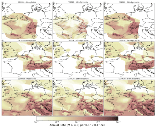
Figure 13 Grids of activity rates for M≥4.5 for FR2020 (a, b, c), DE2016 (d, e, f), and ESHM20 (g, h, i) in terms of mean rate (a, d, g), 16th percentile (b, e, h), and 84th percentile (c, f, i).

Figure 14 Interquartile ranges of activity rates from each source model logic tree: FR2020 (a), DE2016 (b), and ESHM20 (c).

Relative differences between the models can be quantified from this same characterisation via the use of difference maps, both for the mean activity rates (Fig. 15, top) and for the relative differences in the model range shown by the ratio of the interquartile ranges (Fig. 15, bottom). The difference maps present a somewhat incoherent picture, which is not unexpected given the complexities and variations in the constituent source models. We note that in the presentation of the relative comparisons in Fig. 15 (and in subsequent figures), we do not identify any specific model as a reference and instead show all combinations.

Figure 15 Relative increase (in %) between the mean activity rate grids for each model comparison (a, b, c) and the increase in interquartile range (%) (d, e, f): FR2020/DE2016 (a, d), ESHM20/DE2016 (b, e), and ESHM20/DR2020 (c, f).

4.2 A non-parametric statistical approach

Comparisons of the mean and quantiles of the rate distributions such as those shown in Figs. 13 and 15 are certainly important as they highlight regions where the underlying source models have a general tendency toward increased or reduced activity. However, these metrics alone do not necessarily provide insight into the complete similarity or dissimilarity of the full distributions of activity rate divergence or how this divergence varies geographically. To visualise this sort of information we can instead adopt metrics from information theory to help quantify dissimilarity between distributions: weighted Kolmogorov–Smirnov statistic (D_KS) (e.g. Monohan, 2001) and Wasserstein distance (D_WS) (Vaserstein, 1969). If ${\mathit{\lambda }}_k(\mathit{\varphi },\mathit{\theta },m_{\min })$ is the rate grid for source branch k, with weight w_k we can then define for each complete source model logic tree a probability distribution $f_{\mathrm{MODEL}}\left({\mathit{\lambda }}_k\right|\mathit{\varphi },\mathit{\theta },m_{\min })$ at each location, where ${\mathit{\lambda }}_k|\mathit{\varphi },\mathit{\theta },m_{\min }$ is the total activity rate in the spatial domain (ϕ,θ) greater than or equal to a specified minimum magnitude m_min. In the simplest case the spatial domain refers to each grid cell; however, this same process applies to any spatial subdomain of the region enclosed by the original rate grid and could be applied to larger regions or somehow coarsened with respect to the grid. If $f_{{\mathrm{MODEL}}_{\mathrm{A}}}\left({\mathit{\lambda }}_k\right|\mathit{\varphi },\mathit{\theta },m_{\min })$ and $g_{{\mathrm{MODEL}}_{\mathrm{B}}}\left({\mathit{\lambda }}_k\right|\mathit{\varphi },\mathit{\theta },m_{\min })$ are the respective empirical probability density functions for the two full seismic source models A and B implied by their logic trees, then

$$\begin{array}{}\text{(6)}& \begin{array}{rl}{D}_{\mathrm{KS}}& =\begin{array}{c}\sup \\ {\mathit{\lambda }}_k\end{array}\left|F_{{\mathrm{MODEL}}_{\mathrm{A}}}\left({\mathit{\lambda }}_k|\mathit{\varphi },\mathit{\theta },m_{\min }\right)\right.\\ & \left.-G_{{\mathrm{MODEL}}_{\mathrm{B}}}\left({\mathit{\lambda }}_k|\mathit{\varphi },\mathit{\theta },m_{\min }\right)\right|\end{array}\end{array}$$

and

$$\begin{array}{}\text{(7)}& \begin{array}{rl}{D}_{\mathrm{WS}}& ={\int }_{-\mathrm{\infty }}^{\mathrm{\infty }}\left|F_{{\mathrm{MODEL}}_{\mathrm{A}}}\left({\mathit{\lambda }}_k|\mathit{\varphi },\mathit{\theta },m_{\min }\right)\right.\\ & \left.-G_{{\mathrm{MODEL}}_{\mathrm{B}}}\left({\mathit{\lambda }}_k|\mathit{\varphi },\mathit{\theta },m_{\min }\right)\right|d{\mathit{\lambda }}_k,\end{array}\end{array}$$

where $F_{{\mathrm{MODEL}}_{\mathrm{A}}}$ and $G_{{\mathrm{MODEL}}_{\mathrm{B}}}$ are the respective empirical cumulative density functions of models A and B. The conceptual definitions of these terms are illustrated in Fig. 16, where we can see D_KS as the maximum absolute distance between the empirical cumulative density functions (CDFs) and D_WS as the total area enclosed between the CDFs. D_KS is constrained to the domain [0, 1], with 0 indicating perfect agreement in the CDFs and 1 indicating no overlap in the respective ranges of λ_k, while D_WS is constrained only by a lower bound of 0 (total agreement). By working on the cumulative density functions, both terms account for the distribution of weights in each of the logic trees.

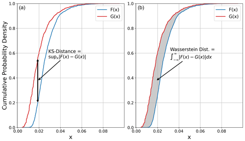
Figure 16 Definition of the Kolmogorov–Smirnov (KS) statistic (a) and Wasserstein distance (b) with respect to empirical CDFs F(x) and G(x).

With D_KS and D_WS we have metrics that allow us to assess spatial variation in the similarity between the effective rate distributions predicted by two different models, which is shown for the combinations of FR2020/DE2016, ESHM20/DE2016, and ESHM20/FR2020 in Fig. 17. The most immediate contrast between the maps using the two different metrics is the apparent “noisiness” of the D_KS metric compared to that of D_WS. The Kolmogorov–Smirnov statistic can appear to change significantly over short distances, often highlighting boundaries of source zones, while Wasserstein distances show a smoother transition, particularly in regions of higher seismicity. The sharp spatial contrasts and variability appear to be particularly exacerbated for comparisons involving ESHM20. This behaviour may be anticipated by the conceptual definitions of the metrics shown in Fig. 16, in which the largest absolute distance between empirical CDFs can change significantly even with relatively small changes in the shape of the CDF. In the empirical CDFs for $F_{{\mathrm{MODEL}}_{\mathrm{A}}}$ and $G_{{\mathrm{MODEL}}_{\mathrm{B}}}$, notable changes in shape may appear from one source zone to another due to changes in the MFRs for each of the zones, while in the case of ESHM20 the comparatively few MFR branches result in empirical CDFs that are more step-like, which results from having gaps in the probability density function (PDF) that can arise due to coarse discretisation of the continuous distributions and/or transitions from one type of source or recurrence model to another. In this respect, D_WS appears to be a better-suited metric for interpretation as it is less sensitive to small changes in the empirical CDFs than D_KS. Focusing on this metric, in the France–Germany border regions we can see more coherent trends, such as greater divergence in the Lower Rhine Graben than along the Upper Rhine for all models, with the ESHM20 providing a notably divergent distribution here. Similarly, the Albstadt Shear Zone emerges as a point of divergence between FR2020 and the other two models.

The rendering of each model into regular rate grids allows us to make comparisons of the source models in a common framework and to interpret differences using simple descriptive statistics as well as through more non-parametric measures that are based on information theory. Here, we contrast the source models from the three different PSHA models (FR2020, DE2016, and ESHM20), though similar comparisons could be made for successive generations of models; however, one need not go back more than one or two generations of regional-scale models before concepts such as the logic tree are no longer found. From the comparisons of the source models shown here, a recommendation would be to compare models firstly via difference maps of mean rates and potentially a small number of selected quantiles and then to apply D_WS to be able to interpret quantitatively how and where the distributions diverge.

Figure 17 Seismicity rate distribution differences between the models given in terms of KS distance, D_KS (a, b, c), and Wasserstein distance, D_WS (d, e, f): FR2020 to DE2016 (a, d), ESHM20 to DE2016 (b, e), and ESHM20 to FR2020 (c, f).

5 Quantitative comparisons of the seismic hazard model results

With the components of the seismic hazard models compared in the previous section, the obvious endpoint to this analysis is to make a comparison of the distribution of the seismic hazard results. To make such comparisons, we limit the area of investigation to the France–Germany border region, stretching from the border with Switzerland in the south to the Luxembourg border in the north. The focus is now limited to this region as it is only here that we have sufficient overlap between all three models to capture contributions from sources up to the stated integration distance of 200 km. Although the Lower Rhine Graben to the north is also of critical importance for understanding seismic hazard in Germany, this region is located at the very eastern extreme of the source models for France; thus the FR2020 sources do not provide complete coverage. Seismic hazard calculations have been run using the OpenQuake engine implementations of each model for a target region enclosed by 47–50.5° N and 5–9.5° E, with target locations spaced every 0.05° (≈ 5.5 km spacing NW and ≈ 3.5–3.7 km spacing EW). Mean hazard and its respective quantiles are calculated using the arithmetic mean of the probabilities of exceedances rather than the levels of ground motion. Hazard curves are determined for all model PGAs and spectral accelerations at periods between 0.05 and 3.0 s. Seismic hazard maps and corresponding difference maps for the 10 % probability of exceedance in 50 years are shown for three intensity measures (PGA, Sa (0.2 s) and Sa (1.0 s)) in Fig. 18.

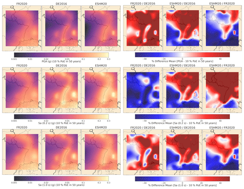
Figure 18 (left) Probabilistic seismic hazard maps covering the France–Germany border region for PGA (top row), Sa (0.2 s) (middle row), and Sa (1.0 s) (bottom row) for 10 % PoE in 50 years. (right) Corresponding difference maps for the hazard comparing FR2020/DE2016 (right column), ESHM20/DE2016 (middle column), and ESHM20/FR2020 (right column).

As we have seen for the distributions of activity rate, comparisons of the resulting hazard maps for means and quantiles only reflect part of a larger picture. Instead, we can also frame the concept of similarity in hazard at a given probability of exceedance in terms of similarity or dissimilarity in the full distribution of hazard values emerging from the logic tree. Once again, we can invoke the two distances (D_KL and D_WS) as measures of dissimilarity for a given ground motion level, A, with a P % probability in T years. In addition, we consider a third metric developed by Sum Mak (personal communication, 2020), which we refer to as overlap index (OI). The OI is illustrated conceptually in Fig. 19 for the distribution of ground motions from the FR2020 and DE2016 models. The distribution of hazard (represented here as PGA with a 10 % probability of exceedance in 50 years) is rendered into a histogram, with the weight of each value corresponding to its branch weight from the logic tree. OI between the distributions of seismic hazard from two different PSHA models at a given probability of exceedance is calculated from

$$\begin{array}{}\text{(8)}& \mathrm{OI}={\int }_{x}min\left(f\left(x\right),g\left(x\right)\right)\mathrm{d}x,\end{array}$$

where f(x) and g(x) correspond to the observed probability densities of ground motion values for the two models respectively. As with D_KS, OI is bounded in the region [0, 1], but here 0 indicates no region of overlap between the models, and 1 indicates perfect agreement.

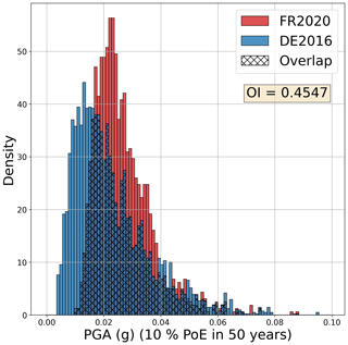
Figure 19 Illustration of the overlap index (OI) between the distribution of hazard at a site using the FR2020 and DE2016 models.

The spatial distribution of dissimilarity between the full hazard models (in terms of the 10 % probability of exceedance in 50 years) can be mapped using the three metrics (D_KL, D_WS, and OI) shown in Figs. 20 and 21. The different maps reveal several interesting features about the differences in the models in this region. Along the main channel of the Rhine as it forms the border between France and Germany from Basel to near Karlsruhe, both D_KS and D_WS measure less dissimilarity between the ESHM20 and DE2016 models, while for these same two models the OI finds less overlap along much of the entire Rhine Graben. Differences between the FR2020 and other models are clearly period dependent in the same region, with the Upper Rhine Graben seemingly in good agreement with other models for PGA and Sa (1.0 s). Yet, for Sa (0.2 s), this same region is clearly illuminated as an area of significant disagreement. Dissimilarity seems to be lower in the northwest of the target region close to the France–Luxembourg border, while it is in most cases at its greatest in northern Switzerland. The Albstadt Shear Zone in the southeast is once again clearly highlighted, with the divergence between the FR2020 and other models clearly visible.

The hazard maps and the corresponding dissimilarity maps show how the distributions of seismic hazard for a given intensity measure type (IMT) and return period change with space, but these should also be complemented with more in-depth comparisons of the hazard curves and uniform hazard spectra (UHS) at specific locations. In Fig. 22 we show two such comparisons for the cities of Saarbrücken (49.23° N, 7.0° E), in an area of lower hazard, and Strasbourg (48.58° N, 7.76° E), which is located in the region of higher hazard along the Upper Rhine Graben. Here, the full seismic hazard curves, including the mean, 16th percentile, and 84th percentile, are shown for Sa (0.15 s) (a period close to the peak of the UHS), alongside corresponding UHS for a 10 % and 2 % probability of exceedance in 50 years. Saarbrücken is located in a region that, as inferred from Figs. 20 and 21, shares a similar seismic hazard distribution in the FR2020 and ESHM20 models but is notably lower in DE2016, while Strasbourg lies about halfway along the Upper Rhine Graben, a region where all three models seem to agree with one another. If we recall the comparison of the URG source zone in Sect. 2 (Fig. 6) and the differences between the recurrence models for the three PSHA models found therein, the degree of agreement between the three models for Strasbourg is somewhat surprising. For both return periods the mean curves and UHS predicted by each model fall within the 16th to 84th percentile of each of the others. Though this is illustrative of the considerable range of ground motion values described by the 16th to 84th percentile, it does suggest a degree of consistency between them that may not be understood if one were to consider solely the changes in mean hazard.

Figure 20 Spatial variation in the dissimilarity between distributions of seismic hazard values for a 10 % PoE in 50 years for PGA (top row), Sa (0.2 s) (middle row), and Sa (1.0 s) (bottom row) using KS distance (left-column set) and Wasserstein distance (right-column set).

Figure 21 As Fig. 20 but considering the overlap index (OI).

6 Discussion and conclusion

The key aim of this study has been to set out a broader perspective of what we mean by comparison in the sense of PSHA models and to illustrate different quantitative techniques to undertake this. Through the examples compared here (FR2020, DE2016, and ESHM20), we consider seismic hazard models that are sufficiently complex for “simple” difference maps to be an insufficient metric of comparison. However, the degree of complexity observed in the models is indicative of the current state of practice, particularly for PSHA in low- to moderate-seismicity regions. Model comparison therefore needs to account for this degree of complexity. In the current analysis we consider three models developed by three separate teams of modellers, each of which worked for different objectives, with different tools, and with a different geographical scope. Under such circumstances it is inevitable that the perspectives on seismic hazard that emerge for a common region (in this case the France–Germany border region) will display a degree of divergence, even if there are many similar elements in each of the models. These can reflect different views as to which uncertainties should be captured by the logic tree and, depending on the tools available, how these uncertainties are evaluated. An important point often overlooked in model comparison is the extent to which the calculation software can influence the actual decisions made by the modeller. The execution of the epistemic uncertainty in the magnitude frequency relation in the three models is a clear example of the complex relationship between tools and modelling decisions and how these can lead to quite different outcomes.

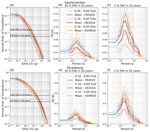
Figure 22 Comparison of the distributions of seismic hazard for Saarbrücken (a, b, c) and Strasbourg (d, e, f) for hazard curves at Sa (0.15 s) (a, d) and UHS for 10 % PoE in 50 years (b, e) and 2 % PoE in 50 years (c, f).

To understand why and how PSHA models for a region diverge, one needs to break down the key factors in the model development and implementation process and analyse each systematically: the input data, modelling approach and philosophy, modelling tools, seismic hazard model components (e.g. seismogenic source model and ground motion model), and – finally – seismic hazard model outcomes. The first two factors are compared in a more qualitative sense than a quantitative one. This is reflected in the presentation of the three models in Sect. 2 of this paper, which juxtaposes the approaches the three different models have taken to represent the seismogenic sources, to model the recurrence of earthquakes from each source, and to capture the expected ground motions from each earthquake. Each of the three models works from input data that share many common characteristics, such as the earthquake catalogue, which for ESHM20 comprises data from both the FCAT-17 catalogue and the input seismic catalogue used by DE2016. Likewise, all three models had available geological data for active faults in both the Upper Rhine Graben and the Lower Rhine Graben, and these have been discarded, partly integrated, or fully integrated depending on the model. In terms of the modelling approach and philosophy, however, it is interesting to note the many places in which the models have largely adopted a similar philosophy, yet the respective implementations yield substantially different outcomes. A key example of this is the use of large-scale area zones (LASZs) based on tectonics and smaller-scale area zones based on local seismicity or geological features, both of which are balanced against a smoothed seismicity model. The LASZs then form the prior zones or direct measurements for the MFRs of the small area source zones within the maximum likelihood estimation, the outcomes of which are distributions of a and b values and their covariances. However, each model differs in the specific zonations and in how the MFRs are, first, fit to the data and, second, mapped onto branches of a logic tree.

One of the main opportunities that emerged from this work was to have all three models implemented in a common format for use with the OpenQuake engine seismic hazard and risk calculation software. This served several purposes, one of which being to understand to what extent the three models differ by virtue of the calculation engine used to run them. The migration process of a PSHA model from one software tool to another is seldom a trivial issue. Discrepancies emerge in computational implementation of the PSHA calculations from one software to the next, which we separate into the following categories: (i) irreconcilable differences in operation, (ii) bugs/errors and/or differences of interpretation, and (iii) configurable parameters. Migration of an implemented or existing model from one software to another is therefore a time-consuming process that focuses on the finest details of the PSHA calculation rather than on the general strategy for source and ground motion modelling.

Model migration differs from dual implementation, a practice that is becoming more widely adopted for quality assurance for critical facilities. This approach executes models in multiple software programmes side by side, identifying discrepancies that are then discussed and potentially resolved (e.g. Bommer et al., 2015; Aldama-Bustos et al., 2019). Migration assumes a reference seismic hazard output from the original software, which the target software aims to reproduce regardless of whether the calculation processes of the original software are deemed optimal. As perfect agreement in the calculations is rarely, if ever, achievable, we can only define agreement between the implementations of a model in its original software and those in the target software in terms of a degree of mismatch over an APoE range of relevance for application. We adopted ±10 % for APoE ≥ 10⁻⁴ (return period ≈10 000 years) for this purpose, which applies first at a branch-by-branch level and then in terms of the mean and quantiles. For DE2016 the target agreement was achieved for the mean and upper quantiles of seismic hazard for the vast majority of sites considered and across multiple spectral periods. In some cases, the OpenQuake implementation estimated lower quantiles that exceeded those of the original software beyond the specified target range. For FR2020 the target agreement could be achieved for all area source branches individually; however, for the smoothed seismicity branches the OpenQuake hazard curves appeared to be on average 20 %–30 % higher over the APoE range of interest. This resulted in OpenQuake's estimations of the mean and quantiles to exceed those of the original software by between 10 %–20 % depending on the location and period, which does not meet the target agreement. At the time of writing, no specific cause for this disagreement had been identified, and we hope that this may still be resolved in subsequent iterations of the model.

The process of model migration for FR2020 and DE2016 was greatly facilitated in this case by the authors of the original models, who supplied us with digital files of both the software inputs and the resulting seismic hazard curve outputs. Despite this, each migration took several iterations, with more information regarding the calculation details needed as each discrepancy was identified and, where possible, resolved. In both cases the specific details of the calculations were not found in the accompanying documentation to the model and required clarification from the authors. In several cases the points of clarification were related to not only small details of implementation but also major differences in how the models were being executed within the calculation, sometimes even contradicting the supporting literature for the model. Though we are sincerely grateful for the input of the model authors in aiding this migration, this highlights a larger problem of model reproducibility and a lack of standardisation in PSHA model documentation. One recommendation for improving practice here would be to require that where PSHA models are intended for use in large-scale applications (e.g. a seismic design code), the digital input and output files for the calculation are made available. In addition, a standard documentation template may be developed that requires the modellers to specify explicitly how the software they are using implements each component of the PSHA model, which parts of the process are configurable, and what values are adopted. Such information could greatly reduce the effort in model migration and ensure greater transparency in the entire PSHA model implementation.

With the FR2020 and DE2016 models migrated to OpenQuake with a satisfactory level of agreement, we have a consistent framework within which we can make quantitative comparisons of the hazard models, both in terms of the fundamental components of the model inputs (i.e. the source and ground motion model) and in terms of the resulting hazard outputs. The latter describes the extent to which models differ, while the former provides insights into why they differ. The key issue we have sought to address in the comparisons is the growing complexity of the logic trees, which means we must now describe both the hazard model inputs and the hazard model outputs in terms of probability distributions and model space. This is the fundamental difference between the current generation of PSHA models in Europe and many of their predecessors. The logic trees of each of the three models considered here incorporate not only alternative source models but also multiple branches for epistemic uncertainty in the magnitude frequency relation. This results in a much larger number of alternative predictions of activity rate and magnitude recurrence (400 for FR2020 and 200 for DE2016), which begin to better resemble probability distributions (albeit of no specific functional form) rather than individual alternative models. We have illustrated here how we can compare models in this context quantitatively, first by looking at metrics describing the centre and variance of the distributions and then by invoking more information theoretic metrics that quantify the proximity of different probability distributions in model space, such as Kolmogorov–Smirnov distance (D_KS) and Wasserstein distance (D_WS). Combining these different metrics and exploring their spatial trends can help provide insight into where the models are most divergent, which can help identify where future efforts could be focused to improve consistency across models in future generations of seismic hazard models for Europe.

This last point takes us toward a critical question that we believe emerges from the work and affects how we may use the models in practice. What can we do to effectively harmonise multiple seismic hazard models that cover a region? This question is not necessarily a scientific one but rather a procedural one. Multiple groups developing separate models for a region and making individual modelling decisions will inevitably result in different estimates of seismic hazard. This is widely recognised, and procedures such as those adopted by the Senior Seismic Hazard Analysis Committee (SSHAC) (Ake et al., 2018) are intended specifically to formalise the management of information and scientific review in order to define the set of technically defensible interpretations and ensure that their centre, body, and range are adequately represented. Seismic hazard modelling in Europe (illustrated here for FR2020, DE2016, and ESHM20) does not currently take place within such a framework, as each model has been commissioned for different purposes and by different organisations with no designation of a body to oversee coordination. ESHM20 aimed to integrate components of both the FR2020 model and the DE2016 model, yet practical limitations, the desire to incorporate new data and developments in PSHA, and the need to create a harmonised model at a larger scale prevented it from faithfully incorporating all elements of the existing models into its framework. Divergence is therefore ensured from the very beginning of this process. Efforts such as the European Facilities for Earthquake Hazard and Risk (EFEHR) are seeking to provide a community structure to hazard and risk modelling around which data and tools are made openly available, and its working groups aim to focus on broadening the discussion of key issues and challenges for modelling. EFEHR cannot necessarily act in the role of technical integrator to the various organisations with remits to model hazard and risk in their respective countries, but it can and does provide harmonised datasets and tools for use as well open-source implementations of hazard and risk, all combined with extensive documentation. These can facilitate harmonisation from the bottom up, eventually moving differences in modelling decisions, alternative interpretations, and parameter uncertainties into a broad distribution of technically defensible interpretations across a region. We hope that if the EFEHR community is successful and can continue to expand, divergence between the models may eventually be minimised to better reflect the actual epistemic uncertainty in a region.