Estimating ground motion intensities using simulation-based estimates of local crustal seismic response

It is estimated that 2 billion people will move to cities in the next 30 years, many of which possess high seismic risk, underscoring the importance of reliable hazard assessments. Current ground motion models for these assessments typically rely on an extensive catalogue of events to derive empirical ground motion prediction equations (GMPEs), which are often unavailable in developing countries. Considering the challenge, we choose an alternative method utilizing physics-based (PB) ground motion simulations and develop a simplified decomposition of ground motion estimation by considering regional attenuation (Δ) and local site amplification (A), thereby exploring how much of the observed variability can be explained solely by wave propagation effects. We deterministically evaluate these parameters in a virtual city named Tomorrowville, located in a 3D-layered crustal velocity model containing sedimentary basins, using randomly oriented extended sources. Using these physics-based empirical parameters (Δ and A), we evaluate the intensities, particularly peak ground acceleration (PGA), of hypothetical future earthquakes. The results suggest that the estimation of PGA using the deterministic Δ−A decomposition exhibits a robust spatial correlation with the PGA obtained from simulations within Tomorrowville. This method exposes an order-of-magnitude spatial variability in PGA within Tomorrowville, primarily associated with the near-surface geology and largely independent of the seismic source. In conclusion, advances in PB simulations and improved crustal structure determination offer the potential to overcome the limitations of earthquake data availability to some extent, enabling prompt evaluation of ground motion intensities.

1 Introduction

The United Nations Human Settlements Programme (UN-Habitat) forecasts that by 2050 some 2 billion new citizens will move to urban centres so that, by then, some 68 % of the world's population will live in cities (United Nations, 2022). It is estimated that 95 % of this urbanization will happen in the Global South. Urban population growth is often accommodated by rapid urban expansion in areas with well-documented seismic risk. The problems of understanding and reducing disaster risk in such rapid development are significant, and while this expansion presents a major global challenge, it also provides a time-limited opportunity to provide evidence-based decision support for this new development (UNISDR, 2015). Efforts in earthquake risk reduction through urban planning guided by high-resolution hazard assessment could reduce disaster risk for hundreds of millions of these future citizens. This approach also provides a cost-efficient method by concentrating on new constructions, where the expenses related to implementing effective earthquake-resistant design and construction are significantly lower compared to the costs of retrofitting at a later stage.

Seismic hazard analysis informs building codes, constraining the construction of new development in earthquake-prone areas through the development of ground motion models (Baker et al., 2021; Bradley, 2019; McGuire, 2008; Stirling et al., 2012; Stirling, 2014; Kramer and Mitchell, 2006; Kramer, 1996). Observed ground shaking is a result of the interaction between a range of individually heterogeneous fields and processes, leading to great complexity in even the simplest relationships. Measures of ground-shaking intensity, for example, show an expected systematic decrease with the distance between the observation and source, but the systematics are overprinted by the interactions between the complexities of the event and the crustal volume explored by the seismic-wave train. The result is high-amplitude variability in the observed intensity. Note that the uncertainty in the observations, in either intensity or distance, makes only a small contribution to this variability; the variability is an intrinsic part of the process.

Consider a series of events recorded at a large number of sensors. In the commonly applied approach, the analyst chooses a functional form for the systematic decay of intensity and uses some fitting procedures to estimate its parameters. The resulting model is commonly known as a ground motion model (GMM) (Douglas and Edwards, 2016; Douglas and Aochi, 2008) and takes the form

$$\begin{array}{}\text{(1)}& \mathrm{lnIM}={\mathit{\mu }}_{\mathrm{lnIM}}+{\mathit{\sigma }}_{\mathrm{lnIM}}\cdot \mathit{ϵ},\end{array}$$

where IM is the required intensity measure, μ_lnIM is the estimated mean-field intensity, σ_lnIM is an estimate of the variability around the mean that is usually assumed to conform to a log-normal distribution and ϵ is the standard normal variate.

It is important to note that the μ_lnIM term does not just describe the attenuation of intensity with distance. Common forms of μ_lnIM attempt to parameterize descriptions of the physics of the entire process, including source properties, such as the focal mechanism and the resulting directivity, as well as the local response of the site using estimates of V_s30 (time-averaged shear-wave velocity in the top 30 m) and κ (high-frequency attenuation parameter), for example (Shi and Asimaki, 2017; Aki, 1993; Bradley, 2011; Kaklamanos et al., 2013; Hough and Anderson, 1988; Borcherdt and Glassmoyer, 1992). Expressions for μ_lnIM in current GMMs include numerous parameters, use advanced statistical techniques to fit these complex functions and represent a practical approach to a fundamentally intractable problem (Douglas and Edwards, 2016).

In practice, an ergodic assumption is invoked in GMM development by aggregating the data from multiple spatial locations that are assumed to be equivalent to the distribution in time (Anderson and Brune, 1999). However, with the increasing data for a particular tectonic area, the non-ergodic or partial non-ergodic approaches are favoured, modifying μ_lnIM and σ_lnIM based on calibration with the local data that are available (Stewart et al., 2017; Bradley, 2015; Rodriguez-Marek et al., 2014). It is observed that a major component of ground motion amplification can be associated with the local geological factors, e.g. sedimentary basins (Graves et al., 1998; Zhu et al., 2018; Pilz et al., 2011), surface topography (Maufroy et al., 2012; Wang et al., 2018; Lee et al., 2009) and soil conditions (Bazzurro and Cornell, 2004; Cramer, 2003; Torre et al., 2020). Hence, the general practice in GMM development is dominated using near-surface site-specific parameters (for example V_s30 and κ). It is suggested that these near-surface parameters might exhibit strong correlations with geological features at greater depths, like basin depth parameters (Z_xx) (Chiou and Youngs, 2014; Tsai et al., 2021; Kamai et al., 2016), and consequently the amplification. However, opposing studies show that the amplification patterns might not necessarily correlate with these parameters (Castellaro et al., 2008; Mucciarelli and Gallipoli, 2006; Pitilakis et al., 2019), for example, sites with velocity profiles which are not monotonically increasing with depth. This highlights the necessity to investigate more regional geological structure to better understand the complexities of ground motion amplification.

Recently, the advances in computational capabilities and understanding the physical processes have made it possible to use physics-based (PB) simulations for modelling ground motions (Smerzini and Villani, 2012; Taborda and Roten, 2014; Bradley, 2019; Graves and Pitarka, 2010). PB simulations are carried out by numerical modelling of the entire process of rupture characterization and seismic-wave propagation through the earth's potentially complex crust. However, the high computational cost and complex input requirements associated with them restrict the large-scale usage of these methods, particularly in 3D. As a consequence the relative contribution of these processes to the total observed variability has been relatively unexplored compared to that of local shallow (decametre) site conditions.

Two immediate problems emerge in enacting the current approaches to ground motion modelling in the context of rapid urbanization in the Global South described above. Firstly, understanding ground motion requires extensive seismic databases recording appropriate measures of intensity from a large number of earthquakes recorded with a network of sensors in the area of interest, for example, the Pacific Earthquake Engineering Research Center Next Generation Attenuation (PEER NGA) databases (Ancheta et al., 2014; Spudich et al., 2013; Atkinson and Boore, 2006). Such catalogues necessitate the deployment of seismometers for many years, even in the most seismically active areas for which is not possible to address the current time-critical problem (Freddi et al., 2021). Secondly, urban development projects require hazard information at unusually high resolution. Urban flood modelling and landslide susceptibility estimates, for example, typically strive to use digital terrain models with 2 m resolution supplemented by high-resolution geotechnical assessments (Jenkins et al., 2023). Seismic intensity also varies significantly over the scale of interest for urban planning, particularly where development is planned over sedimentary basins or near to coasts or rivers with strong spatial contrasts in subsurface seismic velocity (Bielak et al., 1999; see also, Cadet et al., 2011; Foti et al., 2019). Some efforts have been made to incorporate these factors into ground motion prediction equations (GMPEs; Chiou and Youngs, 2014; Campbell and Bozorgnia, 2014; Abrahamson et al., 2014; Marafi et al., 2017); however, the extensive information required to accurately characterize such effects remains a challenge. As a result, the potential for risk reduction with a high cost–benefit ratio that would accrue from a high-resolution understanding of ground motion variability remains elusive. Typically, GMMs developed in data-rich countries of the Global North are reconditioned for deployment in areas for which they have no obvious physical validity (Nath and Thingbaijam, 2011; Hough et al., 2016). At best, this leads to poor spatial resolution precluding the detailed site classification that is critical for seismic microzonation studies needed for cost-effective urban planning (Ansal et al., 2010). The development of appropriate techniques for rapid, local, high-resolution seismic hazard assessment is a significant global challenge.

In this research, we approach this challenge using a simplified decomposition of ground motions into parametric relations explaining the regional and local variations in the measured intensity. We focus on the effects only due to the sedimentary basins, which are known to enhance the amplitude and duration of seismic waves through frequency-dependent focusing, trapping and resonance (Frankel, 1993; Yomogida and Etgen, 1993; Castellaro and Musinu, 2023). We demonstrate the usefulness of PB simulations in capturing the primary low-frequency (LF), < 1 Hz, sedimentary basin effects that contribute to the variation in ground motion within an urban area situated within a seismically active region. We show, to first order, seismic intensity decays along the wave path according to the integrated rheological properties of the region, and this is concurrently subject to relative amplification specific to any point on the surface. We first provide the theoretical physical basis for the decomposition and then describe the simulation domain and the numerical scheme used to explore it. We then describe how the main elements of the problem, i.e. regional mean-field attenuation (Δ) and local site amplification (A) (explained in the subsequent section), can be extracted from the simulations and demonstrate their use in the reconstruction of originally simulated intensities. We highlight that the assessment of these reconstructed intensities is not notably influenced by source characteristics (such as location and directivity). Therefore, calibrating these parameters and understanding short-scale ground motion amplification variability can address the challenge posed by the lack of earthquake data. We suggest that this approach, when extended to include high frequency (HF), might provide an improved relative seismic risk assessment in the form of more reliable microzonation maps at the scale of urban planning, which is based on rapid seismological site characterization in the absence of long-duration seismic catalogues.

2 Theoretical considerations

Using the seismic representation theorem (De Hoop, 1958; Knopoff, 1956), in polar coordinates the displacement U_δ,ε recorded at site ε for point-source earthquake δ is given by

$$\begin{array}{}\text{(2)}& U_{\mathit{\delta },\mathit{\epsilon }}=G_{\mathit{\delta }\left(r,\mathit{\theta },\mathrm{\varnothing }\right),\mathit{\epsilon }}\cdot {\mathit{f}}_{\mathit{\delta }\left(r,\mathit{\theta },\mathrm{\varnothing }\right)},\end{array}$$

where r is the distance between the source and receiver, θ and ∅ are the positional angles in a spherical coordinate system, f_δ is a force vector at δ, and G is the elastodynamic Green's function providing the displacement at ε due to f_δ. Since we consider the peak displacement in an elastic medium in what follows, this equation is time invariant.

Consider a receiver at point ε that experiences displacements due to sources of a given seismic moment at point δ (see Fig. 1). The average logarithm of the peak displacement field for all possible point sources δ_r at distance r from receiver ε can then be expressed as

$$\begin{array}{}\text{(3)}& \stackrel{\mathrm{‾}}{\ln \left(U_{{\mathit{\delta }}_r\mathit{\epsilon }}\right)}={\displaystyle \frac{\mathrm{1}}{\mathrm{2}{\mathit{\pi }}^{\mathrm{2}}}}{\int }_{\mathrm{0}}^{\mathit{\pi }}{\int }_{\mathrm{0}}^{\mathrm{2}\mathit{\pi }}\ln \left(U_{\mathit{\delta }\left(r,\mathit{\theta },\mathrm{\varnothing }\right),\mathit{\epsilon }}\right)\mathrm{d}\mathit{\theta }\mathrm{d}\mathrm{\varnothing },\end{array}$$

where $\stackrel{\mathrm{‾}}{\ln \left(U_{{\mathit{\delta }}_r\mathit{\epsilon }}\right)}$ then represents the expectation value for the intensity at ε due to all possible events at distance r. In this formulation, we consider point sources without any particular focal mechanism, so Eq. (3) might be considered an integration over all possible focal mechanisms at all possible points on the hemisphere.

Figure 1 A cuboidal domain having a receiver at ε and a seismic point source at $\mathit{\delta }(r,\mathit{\theta },\mathrm{\varnothing })$. The top surface of this domain represents receiver field Ω_ε and the volume defines source field Ω_δ. All sources at distance r from ε can be represented as the surface of hemisphere δ_r. These ground motion intensity at ε due to these sources are integrated in Eq. (3). This can further be integrated for all receivers at surface Ω_ε as calculated in Eq. (4).

Integrating over all receivers Ω_ε on the surface of the domain,

$$\begin{array}{}\text{(4)}& \stackrel{\mathrm{‾}}{\ln \left(U_{{\left(\mathit{\delta }\mathit{\epsilon }\right)}_r}\right)}={\displaystyle \frac{\mathrm{1}}{{\mathrm{\Omega }}_{\mathit{\epsilon }}}}\int {\int }_{{\mathrm{\Omega }}_{\mathit{\epsilon }}}\stackrel{\mathrm{‾}}{\ln \left(U_{{\mathit{\delta }}_r\mathit{\epsilon }}\right)}\mathrm{d}\mathit{\epsilon },\end{array}$$

which then provides a mean-field estimate of the expected intensity for any source–receiver pair separated by distance r, and a graph of $\stackrel{\mathrm{‾}}{\ln \left(U_{(\mathit{\delta }\mathit{\epsilon }{)}_r}\right)}$ against r represents the mean-field decay of intensity with distance throughout the entire volume.

The response at a particular location on the surface to any specific event at some distance r will, of course, be subject to the source, path and site effects, all contributing to some local modification of the mean-field expectation. Consider the ground motion at receiver ε due to any source δ; again, peak displacement (U_δ,ε) can be calculated using the representation theorem, this time giving

$$\begin{array}{}\text{(5)}& U_{\mathit{\delta },\mathit{\epsilon }}=G_{\mathit{\delta },\mathit{\epsilon }}\cdot {\mathit{f}}_{\mathit{\delta }}.\end{array}$$

This peak ground displacement U_δ,ε varies with ε, but from Eq. (4), we know its mean across the surface is $\stackrel{\mathrm{‾}}{\ln (U_{\left(\mathit{\delta }\mathit{\epsilon }{)}_r\right)}}$. Normalizing the U_δ,ε by $\stackrel{\mathrm{‾}}{\ln \left(U_{(\mathit{\delta }\mathit{\epsilon }{)}_r}\right)}$ removes the mean-field decay leading to normalized displacement ${\widehat{U}}_{\mathit{\delta },\mathit{\epsilon }}$ given by

$$\begin{array}{}\text{(6)}& {\widehat{U}}_{\mathit{\delta },\mathit{\epsilon }}=U_{\mathit{\delta },\mathit{\epsilon }}/\stackrel{\mathrm{‾}}{\ln \left(U_{(\mathit{\delta }\mathit{\epsilon }{)}_r}\right)}.\end{array}$$

Finally, to encapsulate the effect of all possible sources at each receiver, this normalized displacement can be integrated for the entire source field (Ω_δ), giving

$$\begin{array}{}\text{(7)}& \stackrel{\mathrm{‾}}{\ln \left({\widehat{U}}_{\mathit{\epsilon }}\right)}={\displaystyle \frac{\mathrm{1}}{{\mathrm{\Omega }}_{\mathit{\delta }}}}\int \int {\int }_{{\mathrm{\Omega }}_{\mathit{\delta }}}\ln \left({\widehat{U}}_{\mathit{\delta },\mathit{\epsilon }}\right)\mathrm{d}\mathit{\delta }.\end{array}$$

This $\stackrel{\mathrm{‾}}{\ln \left({\widehat{U}}_{\mathit{\epsilon }}\right)}$ describes a local normalized amplification expected at any point for all possible sources. This can be considered the integrated effect of the whole wave path from all possible sources that is dominated near ε, where these paths converge. This term introduces the empirical site-specific variability using the normalized intensity of a suite of earthquakes of any magnitude.

Equations (4) and (7) now allow us to express the final estimate of the intensity measure as

$$\begin{array}{}\text{(8)}& \ln \left(\mathrm{IM}\right)=\stackrel{\mathrm{‾}}{\ln \left(U_{{\left(\mathit{\delta }\mathit{\epsilon }\right)}_r}\right)}+\stackrel{\mathrm{‾}}{\ln \left({\widehat{U}}_{\mathit{\epsilon }}\right)}.\end{array}$$

For the sake of simplicity, for an event at i, observed at location j, separated by distance r, lnΔ_r is used to denote the first term, mean intensity decay $\stackrel{\mathrm{‾}}{\ln \left(U_{{\left(\mathit{\delta }\mathit{\epsilon }\right)}_r}\right)}$, and lnA_j defines the second term describing amplification, $\stackrel{\mathrm{‾}}{\ln \left({\widehat{U}}_{\mathit{\epsilon }}\right)}$. Now, Eq. (8) can then be re-written as

$$\begin{array}{}\text{(9)}& {\mathrm{IM}}_{ij}={\mathrm{\Delta }}_r\cdot A_j,\end{array}$$

where IM_ij is a non-specific intensity measure recognizing that the argument so far may be generalized to peak velocity or acceleration. IM_ij then provides an estimate of the intensity of ground motion based on the mean-field expected intensity at distance Δ_r, integrated over the entire crustal volume under consideration, and relative amplification A_j due to the integrated effect of the seismic velocity structure around the site. Both terms on the right-hand side are properties of the crust, regional and local, and do not include extended descriptions of the earthquake source, as we show in the next section. Equation (9) defines the Δ−A decomposition, a static ground motion model that emphasizes local geology rather than the descriptions of the earthquake source.

In practice, mean field Δ and amplification A, can both be calibrated through simulation-based estimates for a given domain; hence the basis is essentially non-ergodic, but it is different than data-based statistically estimated parameters used in typical non-ergodic GMMs (e.g. Landwehr et al., 2016; Kuehn et al., 2019). The spatial coefficients estimated in these non-ergodic model are data-dependent; hence in order to find potential drivers of GM variability in data-sparse regions, there is very little scope to use these models. To clarify, the motivation for the potential use of the Δ−A method is to target the data-sparse regions without the extensive availability of earthquake catalogues.

3 Defining domain and source scenarios for simulations

To explore the behaviour and stability of Δ and A (in Eq. 9) and how they might be estimated in practice, we use a virtual world that allows for the exploration of the ideas in the absence of uncertainty but which allows for the introduction of precisely constrained variability. We use a virtual crustal environment, as shown in Fig. 2a and b, that incorporates a simplified subsurface velocity structure centred on a shallow and a deep river basin overlying a crystalline basement to which simplified velocities have been assigned. The description of the domain includes depth-varying density (ρ), shear wave speed (V_s), primary wave speed (V_p) and anelastic attenuation factors (Q_p,Q_s), and it is determined based on the assumed values of these parameters at the surface of the shallow basin (river channel), deep basin and basement (Brocher, 2005, 2008). The reader is referred to Sect. 3.1 of Jenkins et al. (2023) for detailed description of the crustal domain and earthquake moment distribution. Alternatively, this information is also accessible in the Supplement (Table S1 and Fig. S1).

In the middle of the crustal domain, we locate a virtual urban environment Tomorrowville (Menteşe et al., 2023; Gentile et al., 2022; Cremen et al., 2023; Wang et al., 2023; Jenkins et al., 2023). The geology of Tomorrowville is based on a stretch of the Nakhu River valley on the outskirts of Lalitpur to the south of Kathmandu though the velocity structure described here that extends far to the north and south and does not represent the actual subsurface seismic velocity in the area. Instead, we simply generate a hypothetical near-surface velocity structure representative of any urban settlement located around a river channel set in a deeper and wider sedimentary basin. The depths of shallow and deep basins in Tomorrowville are presented in Fig. 2c and d.

The random distribution of 40 thrust-faulting earthquakes (EQ1 to EQ20 are M_w 6 and EQ21 to EQ40 are M_w 5) is simulated across the domain (see Fig. 2e, f) using an established physics-based solver, SPEED, which uses spectral element method (SEM) for solving the wave propagation equations (Mazzieri et al., 2013; Paolucci et al., 2014; Smerzini et al., 2011). SEM combines the geometrical flexibility of the finite-element method (FEM), i.e. the capability to naturally account for irregular interfaces and mesh adaptivity, with the high spectral accuracy, i.e. the exponential convergence rate to the exact solution that results in a fewer number of grid points per wavelength to maintain low dispersion. The crustal domain has a minimum shear wave velocity of 250 m s⁻¹ and the smallest element size of 200 m with the spectral degree of 4; hence, the simulations are able to resolve for the vibrational periods greater than 0.8 s. Fault plane dimensions are determined using widely used empirical relationships developed by Wells and Coppersmith (1994). Kinematic characterization of rupture model is done based on the model developed by Liu et al. (2006) and Schmedes et al. (2013), in which the correlation between the slip, rise time, peak time and rupture velocity among the sub-faults are derived based on a large ensemble of dynamic rupture simulations of dipping faults. The moment distribution remains same for each magnitude ensemble, but the strike and dip are varied. This distribution of rupture scenarios produces a wide range of expected source directivity for any location. The peak ground acceleration (PGA) maps shown in Fig. S2 and Movie S1 are referred to for the visualization of the source orientation and their corresponding effects across the surface of entire domain. The wavefront evolution for EQ1 can also be found in Movies S2, S3 and S4 of the Supplement as well.

Figure 2 The computational domain used for the simulations and the distribution of earthquake scenarios is shown. (a) The sedimentary basin structure showing a river channel creating a shallow basin with a maximum depth of 500 m located inside a 2 km deep basin (see Jenkins et al., 2023, for details). The grey rectangle represents Tomorrowville (e.g. Cremen et al., 2023; Menteşe et al., 2023), which has been designed to help understand the implications of development decision-making regarding consequent risk to future communities. (b) The extent of the basin geometries using the shear wave velocities in a crustal volume of dimensions 100 km in length, 100 km in width and 30 km in depth. (c, d) The basin depths of shallow and deep basins across Tomorrowville with the building distribution (red polygons). The building distribution is shown to highlight the direct impact of seismicity across the potential future infrastructure. (e, f) The 40 thrust earthquakes with random distributions of dip, rake and strike with EQ21 to EQ40 of M_w 5 and EQ1 to EQ20 of M_w 6 are generated across the domain. The hypocentres are represented by blue stars on the fault surface. The colour distribution across each rupture surface shows the moment release following the kinematic rupture models as developed by Liu et al. (2006) and Schmedes et al. (2013).

The Δ−A decomposition, developed theoretically above (Sect. 2), includes no source variability, whereas any attempt to understand seismic hazard must. The azimuth of the events from the seismometer with respect to the dominant velocity anisotropy introduced by the river basin will also contribute to the expected ground motion variability. The aim of this paper is not to examine the influence of these features on the observed local intensity; that will follow in a later work. Instead, we simply explore the extent to which the relative amplification term, A_j, might act as a usable proxy that, to first order, governs the intensity variation across an urban area, irrespective of the source orientation. This might be considered a lower bound on the skill of Eq. (9) in providing the basis for a static site-dependent ground motion model that might be improved later by the introduction of a source term to be constrained by the structural fabric and stress state around any specific location.

4 Estimation of Δ and A for Tomorrowville

The simulation results are used to estimate Δ for the crustal domain and A for Tomorrowville (Eq. 9). The geometric mean of horizontal components of PGA values are used as an intensity measure for all of the rupture scenarios.

To calculate Δ, we uniformly sample the surface of the crustal domain, which is a practical and computationally inexpensive approach to approximate the integration in Eq. (4). In the entire simulation domain, a random set of 100 recording locations is chosen (see green triangles in Fig. 3a), for which estimates of the PGA are simulated for every event, generating a large number of estimates of the peak amplitude for different epicentral distances giving the data points for events of magnitude 5 and 6 shown in Fig. 3b. We use simple least-squares regression to the decay equation

$$\begin{array}{}\text{(10)}& \left|\left.{\mathrm{\Delta }}_r\right|\right.=a+b\times \ln \left(r+c\right),\end{array}$$

where |Δ_r| is an estimation of the mean-field intensity measure Δ_r (introduced in Eq. 9); r is the epicentral distance; and a, b and c are the empirical parameters evaluated from the data-fitting procedure which might be modified without loss of insight (Fig. 3b). The choice of 100 recording locations for |Δ_r| estimation can have inherent uncertainties based on the selection. For instance, if the stations are predominantly concentrated in the basin, it could result in higher intensities in Fig. 3b, consequently causing an upward shift in the mean-field curve. However, such a scenario would not uniformly sample the entire domain as intended; hence, the current choice of stations seems satisfactory.

Figure 3 (a) A map of the computational domain showing the shallow basin (blue) created by a river channel and a deep basin (red), as well as the location of Tomorrowville (grey). Green triangles indicate the random locations of the 100 virtual seismometers. (b) Points indicate PGA versus the epicentral distance for each of the 40 events at each virtual seismometer, and the curves represent the least-squares estimate of the mean-field amplitude decay for these data.

It should be noted that the regression method chosen here does not distinguish the repeatable (within-event) and non-repeatable (between-events) effects, which is determined the fact that each source used here is characteristically similar and is recorded at the exact same set of receivers. Assuming the entire domain has a homogeneous earthquake distribution, each recording is considered independent, irrespective of whether the seismic energy originated from the same or different sources. The concept of earthquake source homogeneity implies that in a scenario with limited prior knowledge of the tectonics in the area, a reverse faulting earthquake could potentially occur at any azimuth with respect to the city.

We now must turn our attention to the variability in the data around the curves (Fig. 3b) and will focus on the Tomorrowville sub-domain. Note that any numerical uncertainties due to the calculation, conditional on the input geological structure, are negligible compared to the variability observed in Fig. 3b. Hence, given the assumption that the simulation is providing accurate estimates in a virtual setting, each point in Fig. 3b accurately represents the local peak amplitude of waves from a particular event recorded at a single station. To estimate |A_j for any location j, the PGA values from all events are extracted for the Tomorrowville domain (Fig. 4a). The linear interpolation of intensities is used to provide these high-resolution maps, which sample Tomorrowville at an approximate grid spacing of 28 m.

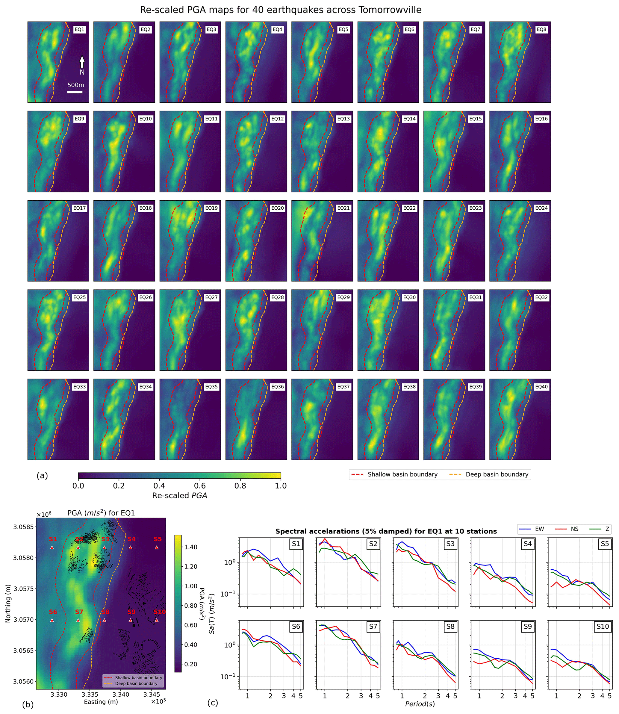
Figure 4 (a) PGA maps for 40 events plotted on the Tomorrowville city domain. EQ1 to EQ20 represent data from M_w 6 earthquakes, while EQ21 to EQ40 are for M_w 5. Note that we have scaled each map between 0 and 1, where 0 is the minimum and 1 is the maximum PGA for each earthquake. The similarity of the maps indicates that, to first order, regardless of the absolute value of the PGA across the zone, the relative amplitude for different locations is invariant. (b) The PGA (geometric mean of two horizontal components) values for EQ1 along with the boundaries of shallow and deep basins, represented by dashed red and orange lines, respectively. Red triangles show 10 stations, S1 to S10, that are used to show the spectral accelerations of 0.8 to 5 s in (c). Three components of east–west (EW), north–south (NS) and vertical (Z) are plotted separately.

As an example, the PGA from earthquake 1 (EQ1) is shown along with the spectral accelerations (5 % damped) at 10 stations, S1 to S10 (Fig. 4b, c). Please note that these receivers are positioned within the Tomorrowville domain and are not accounted for in the wider receiver distribution illustrated in Fig. 3a for the evaluation of |Δ_r|. It can be clearly seen that the basin area is showing strong amplification resulting in higher PGA values due to wave trapping and resonance of the sedimentary basin layers, as compared to the lower PGA values along the areas of the crystalline basement. Spectral accelerations at 10 stations show different orders of amplification over the entire period range (0.8 to 5 s) corresponding to the geological locations of these stations. The consistent decrease in amplitude with an increasing period observed at all stations indicates that it is majorly controlled by the selected source spectra. S2, S3 and S7 lie in the combined (both deep and shallow) basin area (hence, recording the maximum amplification), while S1 and S6 lie above only deep-basin area (hence, the amplification is lesser but still significant at higher periods for all three components). The rest of the stations, S4, S5, S9 and S10, are situated over the basement rocks (hence, recording the lowest value of spectral accelerations).

Our simulations focus on frequencies below 1 Hz due to high computational costs associated with sampling higher frequencies in simulations. However, this analysis remains relevant since basins, like the Kathmandu basin, often exhibit resonance at similar frequencies (Oral et al., 2022; Asimaki et al., 2017). Additionally, when dealing with higher frequencies, it becomes necessary to account for other nonlinear site effects that play a significant role in intensity variations (Semblat et al., 2005), which are not included in this analysis. More discussion on basin resonance is provided in the Supplement (Sect. S1).

Given the geometry of the basin stretched approximately north–south (NS) whilst being much more confined along east–west (EW), the amplification of both horizontal components should be theoretically contrasting. However, the periods resolved in the simulations show the inter-component variability is still lower than the inter-station variability across different geological domains (Fig. 4c). This suggests that the geometric mean of the horizontal components of PGA at each station seems to be a usable guide to explore the amplification further discussed in this study.

The pattern of higher amplification along the river basin and lower amplification along the basement area is common for PGA maps of all the earthquake scenarios (Fig. 4a). Hence while the absolute PGA is strongly dependent on the source magnitude and distance, the relative amplitude within any map is qualitatively independent of the earthquake source orientation and even magnitude. The structural similarity of PGA maps in Fig. 4a seems to indicate the potential utility of the Δ−A decomposition.

To extract this pervasive feature of relative amplification from all earthquake scenarios, we normalize and stack the PGA maps for each event. First, all PGA maps are normalized using the mean smooth-earth expectation value |Δ_r, calculated from Eq. (10). This normalization is the practical implementation of the theoretical description given in the Eq. (6), where the normalization factor is taken as the mean intensity decay in Eq. (4). Let |U_ij be the simulated PGA at a particular site j due to earthquake i at distance r, then the normalized PGA $\left|\left.\widehat{U_{ij}}\right|\right.$ would be

$$\begin{array}{}\text{(11)}& \left|\widehat{U_{ij}}\right|=\left|U_{ij}\right|/\left|{\mathrm{\Delta }}_r\right|.\end{array}$$

After normalization, the average PGA of the normalized maps is calculated for the number of earthquake scenarios N_e, as described in Eq. (7). This final, averaged PGA map is a characteristic spatial kernel for the chosen city domain and theoretically contains the average local amplification (A_j) at any site j for any possible earthquake regardless of source (see Fig. 5a). Here, A_j has the form

$$\begin{array}{}\text{(12)}& A_j={\left(\prod _{i=\mathrm{1}}^{N_{\mathrm{e}}}\left|\widehat{U_{ij}}\right|\right)}^{\frac{\mathrm{1}}{N_{\mathrm{e}}}}.\end{array}$$

The calculation of A_j results in a mean amplification field consistent with the spatial variations observed in the simulations (Fig. 5a). Each pixel represents the mean amplification experienced at that location over all magnitudes, azimuths and directivity.

There is, of course, a dispersion of $\ln \left|\left.\widehat{U_{ij}}\right|\right.$ values around this mean which is itself a spatially variable field over the domain, calculated by ${\mathit{\sigma }}_{\ln \left|\left.\widehat{U_{ij}}\right|\right.}$ (Fig. 5b) as

$$\begin{array}{}\text{(13)}& {\mathit{\sigma }}_{\ln \left|\left.\widehat{U_{ij}}\right|\right.}=\sqrt{{\displaystyle \frac{\mathrm{1}}{N_{\mathrm{e}}}}\sum _{i=\mathrm{1}}^{N_{\mathrm{e}}}(\ln \left|\left.\widehat{U_{ij}}\right|\right.-{\mathrm{lnA}}_j{)}^{\mathrm{2}}},\end{array}$$

where ${\mathit{\sigma }}_{\ln \left|\left.\widehat{U_{ij}}\right|\right.}$ gives the variability due to various source scenarios used in the analysis and the corresponding path effects. The maximum value of ${\mathit{\sigma }}_{\ln \left|\widehat{U_{ij}}\right|}$ is 0.56, which is 23.8 % of the entire lnA_j range of 2.35 in Tomorrowville. The difference of 2.35 in maximum (lnA_j,max) and minimum (lnA_j,min) values would mean that the ratio $A_{j,\max }/A_{j,\min }$ is e^2.35∼ 10.48, implying an order-of-magnitude variation within Tomorrowville. Notably, the ranges of the amplification and standard deviations are of a realistic order often found in some of the extensively studied real-world settings as well, for example as shown by Day et al. (2008) in southern California.

Figure 5 (a) Estimates of lnA_j and (b) the standard deviation (${\mathit{\sigma }}_{\ln \left|\left.\widehat{U_{ij}}\right|\right.}$) for Tomorrowville. Two locations, one in the river basin (S2) and one where the crystalline basement outcrops at the surface (S9), are chosen in (a) to plot the convergence of lnA_j at S2 and S9 with an increasing number of events, as shown in (c).

Another approach to understanding the variability in the amplification field involves varying the number of events used to calculate lnA_j and examining its variability at a specific location using the events selected through a bootstrapping approach. We chose two stations from Fig. 4b, one representing an area of high amplification over the river basin, named S2, and one in low amplification over the outcropping basement, named S9 (see Fig. 5a). The number of events N_c, used to estimate A_j, is plotted against lnA_j, where the colour intensity represents the distribution of the iterations across the entire lnA_j range (Fig. 5c). For each N_c value, 100 random combinations of events with repetition are used for lnA_j calculation. The red dashes correspond to the ±1σ_s2 and ±1σ_s9 variability around the mean lnA_j value for the respective N_c value. The convergence of the lnA_j values can be observed even with as low as about seven events, with a stable ±σ_s2 and ±σ_s9 around the lnA_j values of 0.12 each. This distribution of lnA_j is non-overlapping for both sites S2 and S9, which suggests that the local crustal features at both of these sites are the dominant contributor in the amplification.

5 Estimation of PGA using Δ and A for 40 earthquakes

The theoretical treatment described in Sect. 2 above suggests that the ground motion at a point can be decomposed into the effect of the mean-field attenuation over the wave path integrated over the crustal volume and the effect of the local velocity structure. This implies that the reversal of this process should reproduce the original PGA field. Thus if we have robust estimates of Δ and A, then we should be able to reproduce the intensity at any point using Eq. (9).

We demonstrate this process for a single earthquake, EQ13 located 30.4 km to the NW of Tomorrowville, we will show that the choice of the earthquake is not important. The simulated PGA at every point will be referred to as the true value PGA_true (see Fig. 6a, e). To estimate the PGA value explained in Eq. (9) for this event, referred herein as PGA_ΔA, we first calibrate Δ (Fig. 6b) and A (Fig. 6c) using the rest of the 39 simulated events. Δ and A are multiplied as shown in Eq. (9) to obtain PGA_ΔA values for this earthquake (see Fig. 6d). The difference between PGA_ΔA and PGA_true is calculated and plotted as a residual map (see Fig. 6f). The basin area shows higher negative residuals, suggesting underestimation of PGA_ΔA where PGA_true values are higher, while surrounding the basement exhibits positive values, suggesting overestimation. A graph of PGA_ΔA as a function of PGA_true is shown in Fig. 6g along with the histograms of all the grid points across Tomorrowville. There is a systematic overestimation of PGA_ΔA values for this particular event at the lower-PGA range, and a minor underestimation can be seen on the higher-PGA side. This pattern can be attributed to the characteristic that the lnA_j values, which are used to calculate PGA_ΔA, have mean amplification values spanning a wider range compared to this specific event. The Pearson correlation coefficient (γ) between logarithms of PGA_ΔA and PGA_true is 0.98, suggesting a strong correlation between the two. The histograms presented in parallel to the axes also indicate that the distribution nature of PGA remains preserved across Tomorrowville, exhibiting a tri-modal pattern in both PGA_true and PGA_ΔA (Fig. 6g). This tri-modal pattern is a distinctive influence of three geological domains in the city, the deep-basin area (to the left of shallow-basin boundary), the area comprising both deep and shallow basins, and the basement region.

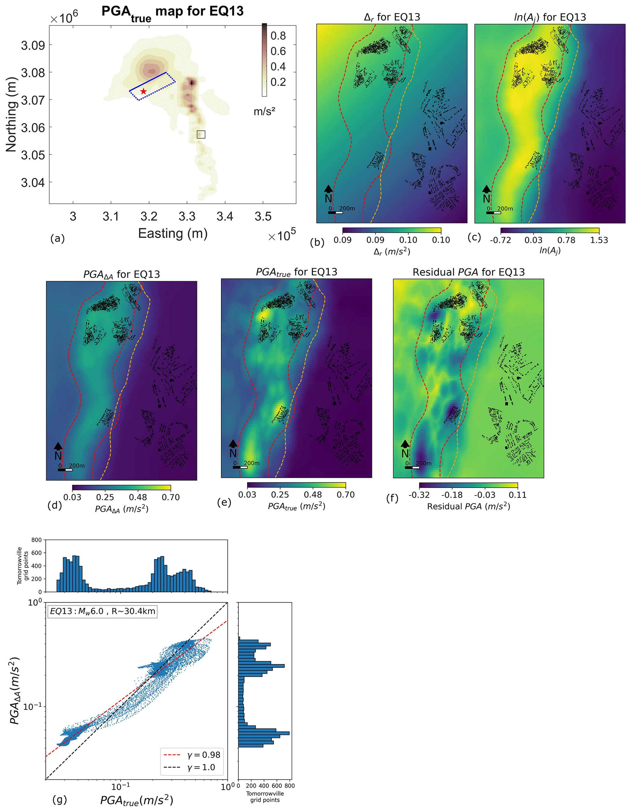
Figure 6 Result showing estimated parameters for EQ13. (a) PGA_true map for EQ13 showing the simulation results across the entire crustal domain, with the dashed blue rectangle showing the location of the rupture surface (top edge is solid blue), red star showing the hypocentre and black rectangle in the middle of domain showing the location of Tomorrowville. (b) Δ_r and (c) lnA_j for EQ13 for Tomorrowville. (d) The PGA_ΔA distribution calculated by multiplying Δ_r with A_j as conceptualized in Eq. (9). (e) PGA_true map for this event obtained through the PB simulation. (f) Residual between PGA_ΔA and PGA_true. (g) The comparison between PGA_ΔA and PGA_true for EQ13 using the Pearson correlation coefficient (γ) of 0.98 for this event. Marginal panels show histograms of PGA_ΔA (right) and PGA_true (top), indicating the similarity in distribution of PGA values across the Tomorrowville city domain.

Finally, for each event in the suite of 40 earthquakes, the remaining 39 simulations are used to calculate Δ and A, which are multiplied to obtain PGA_ΔA. The results are compared with the corresponding PGA_true of each earthquake using the γ value and best-fitting regression line (Fig. 7a). The lowest γ value is 0.89, which suggests that the correlation is strong for all the earthquakes. In conclusion, there is a clear potential of predictability in PGA_ΔA, with some variability translated from different source-specific variability due to the heterogeneous moment distribution along the fault surface, as well as path-related variability due to the azimuth of sources with respect to Tomorrowville. This variability in PGA_ΔA is captured earlier using the ${\mathit{\sigma }}_{\ln \left|\widehat{U_{ij}}\right|}$ values calculated in Fig. 5b.

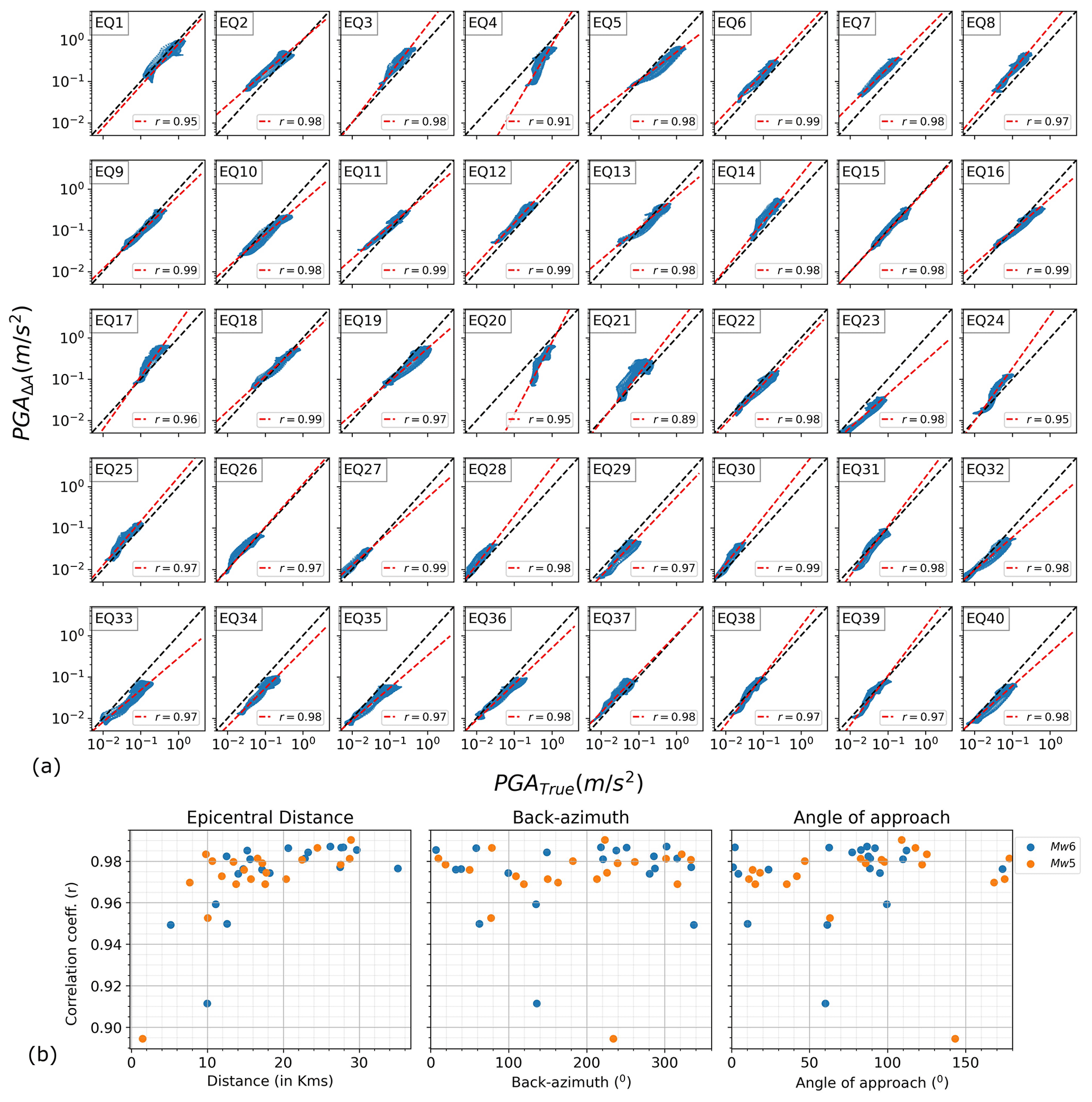
Figure 7 PGA_ΔA is calculated for all 40 earthquakes and compared with the simulated PGA values (PGA_true). (a) The correlation between PGA_ΔA and PGA_true for all earthquakes, where the dashed red line shows the line of best fit and black dashes show the γ=1 line. The γ value is mentioned for all the earthquakes. (b) The γ value versus the distribution of the following three parameters for all 40 earthquakes: epicentral distance, back azimuth (bearing of the line joining the hypocentre to the centre of Tomorrowville) and the angle of approach (the azimuthal difference between the line connecting the hypocentre to the major fault asperity and the line connecting the hypocentre to the centre of Tomorrowville).

The impact of source orientation on the obtained γ value is illustrated by examining three parameters: the epicentral distance, back azimuth of the earthquake (bearing of the line joining hypocentre to the centre of Tomorrowville) and angle of approach (the azimuthal difference between the line connecting the hypocentre to the major fault asperity and the line connecting the hypocentre to the centre of Tomorrowville) (Fig. 7b). The back azimuth and angle of approach provide insights into the influence of the horizontally anisotropic crustal domain and directivity effects resulting from variations in fault orientation relative to Tomorrowville, respectively. γ is observed to have a positive trend with epicentral distance indicating that the earthquakes closer to Tomorrowville are poorly constrained by PGA_ΔA compared to the ones farther away. It can also be seen that the chosen earthquake distribution samples a wide range of values for the back azimuth and angle of approach, indicating a comprehensive representation of these factors. γ does not show any notable trend with the these two factors; hence, their impact on estimating the distribution of PGA values across Tomorrowville is not substantial.

6 Discussion and summary

Estimates from the United Nations Office for Disaster Risk Reduction (UNDRR) suggest that the number of people at risk from a major earthquake will increase from some 370 million in 2020 to more than 850 million by 2050 (United Nations, 2022). Due to historically unprecedented rapid urbanization, these people will be increasingly concentrated in urban centres; the same source estimates that by 2050 global urban population will increase from the current 56 % to around 68 %, with 95 % of this growth happening in the Global South. Without a concerted effort to provide decision support for risk-sensitive construction with a high cost–benefit ratio, ongoing urbanization in areas of high seismic hazard will increase disaster risk for millions.

That the intensity of seismic shaking varies at high spatial frequencies is graphically demonstrated by large differences in seismic damage over very short distances in areas with a uniform building code (Bielak et al., 1999; see also Asimaki et al., 2012; Dolce et al., 2003; Ohsumi et al., 2016; Sextos et al., 2018). What is less well known is the extent to which this variability is the result of differences in the earthquake source or in contrast to the rheological properties of the near surface that might impose a stable and estimable LF amplification, to first order, independent of that source. The former prioritizes forecasting likely earthquake sources in seismic hazard assessment, while the latter suggests that measuring the properties of the near surface might produce a pathway to understanding spatial patterns of seismic shaking regardless of the source. This would in turn open a path to the development of physics-based, high-resolution building-code classification and support evidence-based seismic urban planning policy.

Current methods for seismic hazard assessment require seismic catalogues built from the long-term deployment of large numbers of seismometers to calibrate ground motion models (Douglas and Aochi, 2008; Douglas, 2017; Douglas and Edwards, 2016). The observed variability around these models is assumed to be stochastic, and statistical methods are used to provide the moments of the emerging distributions leading to low-spatial-resolution estimates of seismic hazard. Over most of the Global South such long-term data have not been collected nor is there any current appetite for deploying dense networks of seismometers required for this assessment at the resolution which would be required to guide seismic-risk-informed urban planning at actionable scales.

In this study we have harnessed the potential of high-resolution PB earthquake simulations to explore the extent to which seismic intensity variability might be described by near-surface geology and explained that relative seismic intensity is independent of the earthquake source. Do some areas shake more than others, regardless of the earthquake? We exploit the certainty of a virtual world, Tomorrowville, in which the rheology, described by the geometry of the seismic velocity, is known everywhere; in which seismic sources are precisely described by kinematic models (Graves and Pitarka, 2010; Schmedes et al., 2013); and in which wave propagation is perfectly described by the wave propagation solver (SPEED) we use (Mazzieri et al., 2013). The choice of software should not lead to any notable deviation from the results obtained in this study.

The study develops a Δ−A decomposition that splits the seismic process into a mean-field attenuation model, describing the amplitude decay with source–receiver distance, and an amplification field, describing the integrated amplification of the entire wave path as experienced at each point on the surface. We have shown methods for the estimation of the Δ model and for the A field for Tomorrowville and demonstrated that their description can be used to estimate the true PGA field.

This study utilizes PB simulations in a virtual environment that shows a significant fraction of the observed variability can be explained without categorizing them as stochastic. In the real world, beyond these deterministic variations, stochastic elements of the process must be considered separately. Moreover, it becomes important to classify uncertainties as aleatory or epistemic when the real data guide the model fitting and resulting deviations (Der Kiureghian and Ditlevsen, 2009). However, in this study, PB simulation results are assumed to be devoid of any modelling uncertainties (or aleatory variability), and they are treated as reproducible true solutions in the analysis. Consequently, the deviations obtained in the results of Fig. 7a are fundamentally epistemological. The difference between the amplification map for any event and the A field that determines the value of the local PGA is precisely quantified and accessible. Investigations show that the maximum standard deviation of the A field is about 23.8 % of lnA_j measured across the entire area that includes the source- and path-dependent variability. More importantly, analysis of the variability in the amplification value at any point indicated stable convergence from as few as seven event simulations. Furthermore, comparisons of amplifications at locations over the river basin with locations on the basement in Tomorrowville produced stable, order-of-magnitude differences in amplification which converged rapidly and which gave stable non-overlapping amplification estimates. Of course, both the stability and the contrast in amplification are functions of the choice of velocity distribution, but the choice of the model here was developed to reflect not uncommon velocity geometry, not to accentuate amplification contrasts. We expect that the general conclusions of this work are independent of the details of the Tomorrowville velocity model.

We have not attempted to explore the variability in the amplification with the source parameters, and the initial results suggest that the influence is not likely to be strong. The main candidates expected to be dominant in the strongly anisotropic velocity model used here, source directivity and epicentral azimuth, do not make an appreciable systematic contribution to the A field. Descriptions of active fault geometry and seismotectonics of Tomorrowville could impose a source fabric introducing some systematic influence on the amplification field. Incorporation of any such influence could only constrain the variability, so the results described here might be considered a lower bound on the stability of the A field. The primary factor influencing ground motion amplification in this study is the basin geometry or buried topography, although the impact of surface topography is also anticipated to significantly affect the amplification pattern (Poursartip et al., 2020; Lee et al., 2009; García-Pérez et al., 2021; Geli et al., 1988). The surface topography, often rich in high-resolution data, is the most straightforward to control, and it is expected to contribute to the observed variability. Future research will concentrate on investigating the influence of surface topographic features, in addition to buried topography, on the amplification phenomenon.

The reconstruction of the simulated PGA fields provided further evidence of the efficacy of the method. Using estimates of the Δ and A components from a set of 39 simulations (out of 40) provided strong correlations between true and inverted PGA fields for the 40th. Further, in keeping with the observation of non-overlapping amplification values for basement and basin locations, places with high-intensity shaking were broadly consistently high intensity for all events, whereas locations experiencing low-intensity shaking were also consistent across all events.

The results are suggestive of an underlying physical process in which small-scale LF relative shaking intensity is controlled more by local geology than by source process. Given the description of the relevant fields through simulations, each taking approximately a day on a commonly available computer cluster (see Table S3 for simulation parameters and run-time estimates), it is feasible to estimate the entire PGA field (PGA_ΔA) for an event of a specific magnitude and location in milliseconds of computing time. At a minimum, this provides a workflow through which normal probabilistic seismic hazard assessments that require estimates of PGA for thousands of events at each location can benefit from the advances in PB simulations without the massive compute overhead that makes these computations unfeasible at present.

The stability of the relative amplification field together with the stable, order-of-magnitude difference in PGA across the surface of Tomorrowville demonstrated in this study points to methods for high-resolution seismic hazard estimation based on understanding the static properties of the near surface, rather than on the unpredictable properties of future earthquakes. The challenge becomes a problem of measurement, rather than forecasting. There remains the critical problem either of the elucidation of the velocity structure of the near surface (Sebastiano et al., 2019), so the Δ and A fields might be estimated through simulation as in this paper, or of the direct estimation of the field by measurement of the intensity of shaking at high resolution in the area of interest. To clarify again, this study explores only LF near-surface effects arising from the presence of complex sedimentary basins and shows their contribution in short-scale variability in amplification. It is noteworthy that these LF effects are additional to the site effects related to very near-surface (decametre) depths, which include nonlinear soil responses and other high-spatial-frequency velocity variations, all of which can lead to intricate outcomes (Taborda et al., 2012). Consequently, for applications like enhancing microzonation maps, it is imperative to merge this analysis with elements accounting for HF variability.

In conclusion, rapid urban expansion in areas of poor historical instrumentation leaves significant gaps in data for seismic hazard assessment. Furthermore, current methods both require decade-long deployment of dense seismic networks in the area of near-future urban development and fail to provide high-resolution assessments that identify areas of strong and weak shaking that could underpin seismic-code classification with a high cost–benefit ratio. The potential of PB simulations has prompted the evaluation of the seismic-wave field across areas of near-future development. The results suggest methods to allow for the rapid, high-resolution assessment of geological structure that could lead to risk assessment at unprecedented resolution.