Convection-permitting climate model representation of severe convective wind gusts and future changes in southeastern Australia

Previous research has suggested that the frequency and intensity of surface hazards associated with thunderstorms and convection, such as severe convective winds (SCWs), could potentially change in a future climate due to global warming. However, because of the small spatial scales associated with SCWs, they are unresolved in global climate models, and future climate projections are uncertain. Here, we evaluate the representation of SCW events in a convection-permitting climate model (Bureau of Meteorology Atmospheric Regional Projections for Australia, BARPAC-M) run over southeastern Australia for the months of December–February. We also assess changes in SCW event frequency in a projected future climate for the year 2050 and compare this with an approach based on identifying large-scale environments favourable for SCWs from a regional parent model (BARPA-R). This is done for three different types of SCW events that have been identified in this region, based on clustering of the large-scale environment. Results show that BARPAC-M representation of the extreme daily maximum wind gust distribution is improved relative to the gust distribution simulated by the regional parent model. This is due to the high spatial resolution of BARPAC-M output, as well as partly resolving strong and short-lived gusts associated with convection. However, BARPAC-M significantly overestimates the frequency of simulated SCW events, particularly in environments having steep low-level temperature lapse rates. A future decrease in SCW frequency under conditions with steep lapse rates is projected by BARPAC-M, along with less frequent favourable large-scale environments. In contrast, an increase in SCW frequency is projected under conditions of high surface moisture, with more frequent favourable large-scale environments. Therefore, overall changes in SCWs for this region remain uncertain, due to different responses between event types, combined with historical model biases.

1 Introduction

Damaging surface winds can have large impacts on society and are important to consider in designing buildings and infrastructure. In the mid-latitude regions of southeastern Australia, extreme surface wind speeds (that is, gusts that exceed a 20-year average recurrence interval) tend to be associated with convection (Holmes, 2002), with these events sometimes being known as severe convective winds (SCWs). As discussed by Wakimoto (2001), these events can be divided into two broad classes of related physical processes: firstly, there are convective downdraughts (or “downbursts”) associated with precipitation and evaporative cooling that can transport momentum to the surface (Fujita, 1985; Wakimoto, 1985; Srivastava, 1985; Atkins and Wakimoto, 1991; Geerts, 2001), including in supercell rear-flank downdraughts (Klemp and Rotunno, 1983). Secondly, there are mesoscale downdraught processes, such as bow echoes, derechos, and associated rear inflow jets, that can form as a result of organised convection (Johns and Hirt, 1987; Wakimoto et al., 2006). Both classes of processes can sometimes be embedded within synoptic-scale weather systems, with the vertical mixing of strong winds from aloft having a large contribution to severe surface winds in these situations (Ludwig et al., 2015; Pantillon et al., 2020).

Some of these convective processes may possibly be affected by human-induced climate change. For example, global warming is expected to increase surface heat and moisture availability for deep moist convection and severe thunderstorms, based on estimates of large-scale environmental changes from global climate models (GCMs; e.g. Trapp et al., 2009; Púčik et al., 2017; Lepore et al., 2021) and theoretical changes in the convective environment due to tropospheric warming (Ye et al., 1998; Singh et al., 2017). Future human-induced climate change could also potentially impact other factors relevant for deep moist convection, such as temperature lapse rates, vertical wind shear, and relative humidity (Seeley and Romps, 2015; Chen et al., 2020). Therefore, the frequency of large-scale environments favourable for SCWs is expected to shift in the future but with significant uncertainties related to a wide range of associated processes such as those mentioned above, as well as a relatively limited number of regional studies (Martinez-Alvarado et al., 2018; Brown and Dowdy, 2021a; Prein, 2023). Also, these methods for future projections based on the large-scale environment do not consider potential changes in storm-scale processes that may be sensitive to future warming, such as those related to internal storm dynamics and storm mode, the distribution of hydrometeors, or potential changes in storm initiation mechanisms and convective inhibition (e.g. Hoogewind et al., 2017; Allen, 2018; Raupach et al., 2021). These limitations have resulted in relatively low confidence in future projections of severe thunderstorms and SCWs based on environmental changes (Seneviratne et al., 2021).

To increase confidence in future projections of severe convection, methods based on large-scale environmental changes have recently been complemented by approaches that use convection-permitting atmospheric models, regionally nested within global climate models. These models often show significant improvements in representing convective hazards relative to coarse-scale models, due to partially resolving deep convection (e.g. as reviewed by Prein, 2015). Recent studies have used these convection-permitting models to estimate changes in severe convection and hailstorms in the United States (Trapp et al., 2011; Gensini and Mote, 2015; Trapp et al., 2019; Ashley et al., 2023) and convective rainfall in Europe (Kendon et al., 2017; Chan et al., 2023) and Africa (Kendon et al., 2019), for example. These studies have shown that convection-permitting models can elucidate important details in future projected changes that are not resolved by coarse-scale models and methods. For example, projected decreases in the rate of convective initiation have been reported in the United States but with increases in the intensity of thunderstorms that do occur based on simulated radar reflectivity and updraught speeds (Hoogewind et al., 2017; Haberlie et al., 2022).

A limited number studies have focused on future regional changes in surface wind gusts related to convection using convection-permitting models (Trapp, 2021; Van de Walle et al., 2021; Dowdy et al., 2021; Manning et al., 2023). These studies have suggested potential future increases in the frequency of SCWs but still with significant uncertainties related to a small number of regions and models. In addition, while convection-permitting models might be able to broadly represent convective downdraughts and internal storm dynamics leading to SCWs, as shown previously for individual cases (Hawbecker et al., 2017; Bolgiani et al., 2020), there are often significant errors in the timing, location, and characteristics of severe convection in general (Weisman et al., 2008; Kendon et al., 2021). These errors are likely related to several dynamical processes that are not sufficiently resolved by these model configurations, such as microphysical processes and the entrainment of environmental air (Bryan and Morrison, 2012; Jucker et al., 2020; Bergemann et al., 2022). Errors in convective storm timing and location have also been shown to be caused by deficiencies in boundary conditions in some cases, relating to representations of the large-scale thermodynamic environment (Hanley and Lean, 2021). Also, the turbulent nature of SCW events means that the relevant surface winds are often parameterised in these models (Hawbecker, 2020), which can lead to biases in surface wind speeds. Further, the extent of the abovementioned biases may vary with different physical SCW processes that can have different spatial scales, including the convective-scale and mesoscale processes outlined above. Many of these physical processes are potentially relevant for SCWs in southeastern Australia, as demonstrated by Brown et al. (2023).

This study will further complement recent developments in the climate modelling of severe convection by examining the representation of SCWs in a convection-permitting modelling framework, in southeastern Australia, compared with coarse-scale models and weather station observations. Future projected changes in simulated SCW events will then be assessed and compared with future changes based on the large-scale convective environment. Environmental data will also be used to separate different types of SCW events in the model and in observations to examine potential variations in the quality of model representation and future projected changes between these event types. The paper is structured as follows: firstly, the modelling framework being examined here is introduced, as is the observation-based dataset using station wind gust measurements. Secondly, the intensity distribution for all daily maximum wind gusts over the domain of southeastern Australia is compared between the models and observations. Then, the characteristics of convection-associated severe wind gusts are compared between the convection-permitting model and the observed dataset. This includes an analysis of wind gust duration and strength compared to the background flow, the spatial variability in severe events, and variations in these characteristics between different types of SCW events. Finally, future projected changes in simulated SCW events and favourable SCW environments are presented and compared, before a discussion of the results and concluding comments.

2 Datasets and methods

2.1 Bureau of Meteorology Atmospheric Regional Projections for Australia (BARPA)

The convection-permitting model used here is a part of the broader BARPA modelling framework from the Australian Bureau of Meteorology (Su et al., 2021). BARPA downscales global atmospheric model data to regional domains using the Australian Community Climate and Earth System Simulator (ACCESS), which is based on the Global Atmosphere configuration of the UK Met Office Unified Model. Here, the BARPA hindcast simulations over 1990–2015 covering two nested domains are analysed: firstly, BARPA-R, which is a regional simulation with a domain that covers eastern Australia and, secondly, BARPAC-M, which is a convection-permitting simulation nested within BARPA-R with a domain covering southeastern Australia (Fig. 1). The BARPAC-M simulations were run after the full time period of BARPA-R simulations was completed. BARPAC-M can therefore be considered an offline simulation with no feedback into the BARPA-R simulation. The BARPA-R simulation used here is configured with ACCESS at 12 km horizontal grid spacing, downscaled from ERA-Interim (that is, on a 0.75° latitude–longitude grid; see Dee et al., 2011) at the boundaries with no data assimilation. BARPAC-M is configured with ACCESS on a 2.2 km horizontal grid and therefore does not parameterise deep convection. The BARPAC-M simulations use a sponge zone for the lateral boundary nesting in the BARPA-R simulations, with analysis excluding data from that sponge zone, as was also the case for the BARPA-R simulations nested in ERA-Interim (Su et al., 2021). The BARPAC-M data available for use here cover the months of December–February, over the same years as BARPA-R.

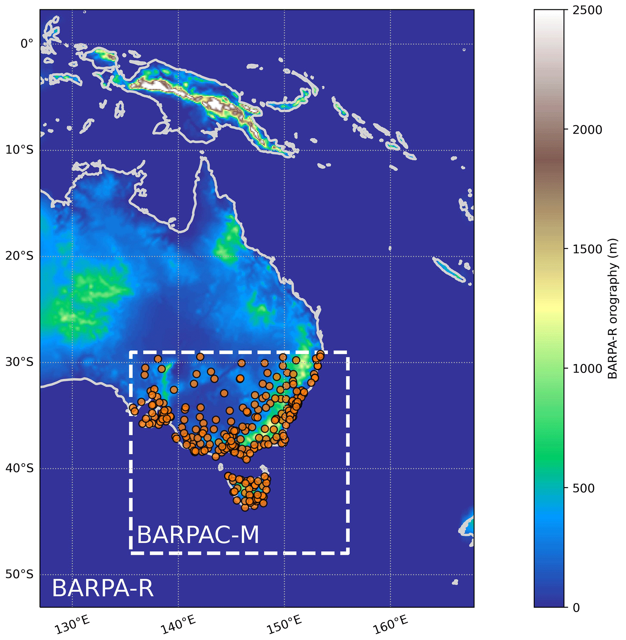
Figure 1 BARPA-R domain, with the inner BARPAC-M domain indicated by dashed white lines. The location of all automatic weather stations used here is indicated with orange circles. Orographic heights used in BARPA-R are shown with shaded contours.

In addition to these hindcast simulations, two 20-year BARPA climate simulations are also analysed. These are downscaled from the ACCESS1-0 global climate model (that is, on a 1.25° × 1.875° latitude–longitude grid; see Bi et al., 2013) under a historical forcing scenario over 1985–2005 and an RCP8.5 (Representative Concentration Pathway) scenario over 2039–2059. Historical and future climate simulations have the same configurations as mentioned above for BARPAC-M and BARPA-R.

In each BARPA configuration, surface wind gusts are parameterised by adding a turbulent component to the predicted 10 m wind speed. This parameterisation is intended to represent a gust defined by 3 s average wind speed, based on the standard deviation of the resolved horizontal wind speed, surface roughness, and stability of the surface layer (Ma et al., 2018). Parameterised 3 s wind gust output is saved at 10 min intervals in both models. For BARPAC-M, the 10 min output represents the maximum 3 s gust over all model time steps. In contrast, for BARPA-R, the 10 min output represents the wind gust from a single model time step, based on a model time step of 5 min. For the purposes of comparing the two model configurations, the BARPA-R 3 s gust distribution based on instantaneous 10 min output is expected to be similar to a 10 min maximum, given the relatively coarse model time step of 5 min but with slightly lower mean and extreme values. This is demonstrated in the Supplement (Sect. S1) by resampling observational wind gust data to 5 min intervals, where a bias of around −1.0 to −0.5 m s⁻¹ is introduced using 10 min instantaneous observed gusts relative to 10 min maximum observed gusts. However, this bias is not expected to significantly impact the analysis of extreme wind gusts associated with convection, where spatial resolution and physical process representation are most relevant when comparing between models (as will be shown in Sect. 3.1 and 3.2).

Lightning flashes are also estimated by BARPAC-M and saved as daily output (number of flashes each day). Lightning flashes are parameterised based on an upwards graupel flux approach, combined with the distribution of ice-phase hydrometeors, which is known to correlate with observed lightning (McCaul et al., 2009). Lightning flashes are matched with BARPAC-M and BARPA-R wind gusts using a radius of 50 km on the same day.

2.2 Observations of wind gusts and convection

Wind gust observations are obtained from a large number of automatic weather stations (AWSs) managed by the Australian Bureau of Meteorology at 272 locations in southeastern Australia (Fig. 1). All available AWSs were used here, except for those located more than 1000 m above sea level and those located offshore. These stations are excluded because of difficulties in identifying convective wind gusts. Wind gusts are reported as the maximum in 1 min intervals and represent a 3 s average wind speed at a height of 10 m. The 10 min maximum of these 1 min observations is taken to match to the BARPA hindcast wind gust data. Automatic quality control information is provided with each wind gust measured by an AWS, with only data that have passed this quality control check retained here. In addition, six instances of erroneously large wind gusts are manually removed based on unrealistic gust evolution and/or gust speeds.

Lightning observations from the World Wide Lightning Location Network (WWLLN Virts et al., 2013) over the period of 2005–2015 are also analysed in relation to severe wind gusts. Lightning flash counts are binned onto a 0.25° latitude–longitude grid, at hourly intervals. The hourly grid values are then resampled to daily sums to match to BARPAC-M parameterised lightning output, and grid cells are matched spatially to station locations with a 50 km radius.

2.3 Environmental diagnostics

Large-scale diagnostics that describe the convective environment and are relevant for SCWs are calculated, using 6-hourly BARPA-R and ERA5 output on pressure and surface levels. These environmental diagnostics will be used for the clustering of different SCW types (see Sects. 3.3 and S2 for further details), as well as for identifying favourable SCW environments in Sect. 4. To identify favourable SCW environments, the Brown and Dowdy (2021b) statistical diagnostic (BDSD) is applied. The BDSD is based on a logistic regression approach that relates environmental variables to the probability of a measured SCW event, in the form

$$\begin{array}{}\text{(1)}& \mathrm{BDSD}={\displaystyle \frac{\mathrm{1}}{\mathrm{1}+e^{-z}}},\end{array}$$

where

$$\begin{array}{}\text{(2)}& \begin{array}{rl}z& =\mathrm{6.1}\times {\mathrm{10}}^{-\mathrm{2}}\left(\mathrm{EBWD}\right)+\mathrm{1.5}\times {\mathrm{10}}^{-\mathrm{1}}\left(\mathrm{Umean}\mathrm{800}\text{–}\mathrm{600}\right)\\ & +\mathrm{9.4}\times {\mathrm{10}}^{-\mathrm{1}}\left(\mathrm{LR}\mathrm{13}\right)+\mathrm{3.9}\times {\mathrm{10}}^{-\mathrm{2}}\left(\mathrm{RHMin}\mathrm{13}\right)\\ & +\mathrm{1.7}\times {\mathrm{10}}^{-\mathrm{2}}\left(\mathrm{SRHE}\right)+\mathrm{3.8}\times {\mathrm{10}}^{-\mathrm{1}}\left(\mathrm{Qmelting}\right)\\ & +\mathrm{4.7}\times {\mathrm{10}}^{-\mathrm{4}}\left(\mathrm{Eff}\text{-}\mathrm{LCL}\right)-\mathrm{1.3}\times {\mathrm{10}}^{\mathrm{1}},\end{array}\end{array}$$

EBWD is the effective bulk wind difference (m s⁻¹), Umean800–600 (m s⁻¹) is the mass-weighted mean wind speed over the 800–600 hPa layer (m s⁻¹), LR13 is the temperature lapse rate from 1–3 km above ground level (°C km⁻¹), RHMin13 (%) is the minimum relative humidity in the 1–3 km layer, SRHE (m² s⁻²) is the effective storm relative helicity, Qmelting (g kg⁻¹) is the water vapour mixing ratio at the height of the melting level, and Eff-LCL (m) is the lifting condensation level of an effective-layer parcel. The effective layer and related quantities are defined following Thompson et al. (2007). Here, following Brown and Dowdy (2021a) a threshold probability of 0.83 is applied to Eq. (1) to classify an environment as being favourable. For further details on the definition and calculation of this diagnostic, please refer to Brown and Dowdy (2021a, b).

Each BARPAC-M wind gust is matched to BARPA-R environmental diagnostics using the most recent 6-hourly time step before the gust and by taking the maximum of each diagnostic in a 50 km radius around the gust location using model land points only, following Brown et al. (2023). Similarly, each observed gust is matched to ERA5 environmental diagnostics using the same method. It is noted that the distribution of relevant environmental diagnostics between ERA5 and BARPA-R is very similar, providing confidence in the use of these diagnostics from BARPA-R (see Sect. S2).

3 BARPA hindcast evaluation

3.1 Daily maximum wind gust intensity distribution

Here we compare the wind gust intensity distribution between each of the BARPA hindcast model configurations, the forcing model (ERA-Interim), and observations measured from AWS. BARPA wind gusts are first subset to grid points that are spatially nearest to each AWS location, using model land points only. BARPA data are only retained at times when neighbouring AWSs are reporting quality data, over a 2005–2015 period using only the months of December–February (with this period representing the overlap between BARPAC-M, BARPA-R, and WWLLN). The daily maximum gust at each station location is then calculated to reduce the number of samples while preserving strong gusts that are of interest here. Daily maximum ERA-Interim gusts are calculated in the same way as each BARPA model described above, noting that ERA-Interim gusts are available as the maximum in 3-hourly intervals. It should be noted that the observations used here are representative of a single point location, compared with each of the model datasets that are intended to represent a grid cell average. Therefore, some differences between the observed wind gust distribution and model distributions should be expected, including lower model wind speeds for local wind gust events at station locations in general. The effect of model grid spacing will be investigated later in this section for BARPAC-M.

Figure 2a shows a wind gust intensity histogram for all daily maximum gusts from each dataset, with Fig. 2b–e showing quantile–quantile plots for each model compared with the observed dataset. ERA-Interim is shown to realistically represent wind gust percentiles up to around 15 m s⁻¹ while significantly underestimating percentiles above this. This is likely due to the large grid cell area of this model dataset, as mentioned above in relation to comparison with point observations. The maximum gust produced by ERA-Interim is around 37 m s⁻¹, which is 7 m s⁻¹ below the maximum observed gust (Table 1). BARPA-R provides an improved gust distribution for the upper tail, with a realistic estimate of wind gust percentiles up to the 99th percentile, equivalent to around 24 m s⁻¹ (Fig. 2d). For percentiles greater than this, BARPA-R tends to underestimate the wind gust speed compared with observations (Table 1). BARPA-R does produce a small number of gusts between 33 and 44 m s⁻¹, although these are all related to the same large-scale low-pressure system produced by the model on a single day. Therefore, the uncertainties associated with the estimate of the maximum wind gust in BARPA-R are relatively large, as demonstrated by dashed lines in Fig. 2d.

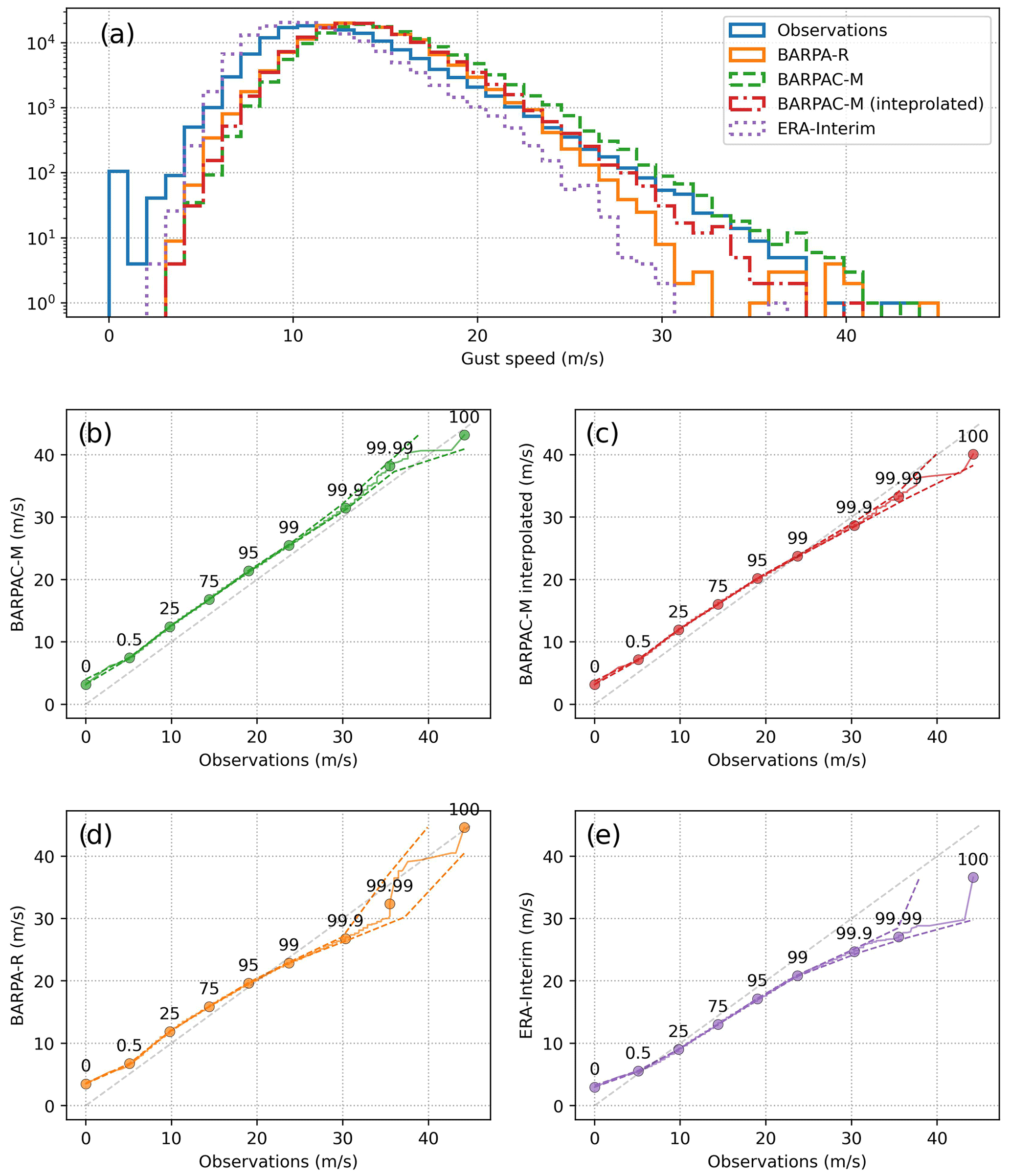
Figure 2 (a) Histogram of daily maximum wind gust intensity over the 2005–2015 period (months of December–February), from the BARPA-R and BARPAC-M hindcasts, the BARPAC-M hindcast interpolated to the BARPA-R grid, ERA-Interim, and station wind gust observations (with a log scale for counts in each bin). (b) Quantile–quantile plot comparing daily maximum BARPAC-M hindcast wind gust percentiles with station wind gust percentiles, with a line plotted using 1000 evenly spaced quantiles up to the 95th percentile and then a number of quantiles equivalent to 5 % of the number of samples plotted from the 95th to 100th percentile. Selected percentiles are also indicated with circle markers and labelled with text. Dashed lines represent a two-sided 95 % confidence interval, calculated by resampling each distribution 1000 times with replacement and determining each of the labelled percentiles. (c, d, e) Same as (b) but comparing BARPAC-M interpolated to the BARPA-R grid, BARPA-R, and ERA-Interim with station wind gusts, respectively.

BARPAC-M tends to overestimate the observed wind gust distribution for most percentiles by around 1–3 m s⁻¹ (Fig. 2b), although with a better representation of the extreme upper tail (above the 99th percentile) compared with BARPA-R. The physical reasons for this improvement are investigated in Sect. 3.2 by analysing convective wind gusts in the model. Here, we also examine the effects of the horizontal grid size on the representation of the daily wind gust distribution by presenting the distribution from the BARPAC-M hindcast that has been regridded to the BARPA-R grid (using a conservative interpolation approach). Regridding leads to a reduction in the overestimation of the gust speed from BARPAC-M for low percentiles and a slight underestimation of wind gusts relative to observations for percentiles exceeding the 99.9th percentile (above 30 m s⁻¹). The regridded BARPAC-M distribution produces higher wind gust percentiles than BARPA-R for the extreme upper tail, closer to observations (Fig. 2c, Table 1). This indicates that added value in BARPAC-M is provided by improvements in relatively small-scale resolved processes, in addition to higher-resolution output.

Table 1 Percentile values of daily maximum observed wind gusts (m s⁻¹) and the bias in each model dataset for those percentiles. A two-sided 95 % confidence interval is shown in brackets, estimated by randomly resampling each model distribution 1000 times, with replacement.

To examine how changes in large-scale forcing could affect the daily maximum wind gust distribution, we also compare the BARPAC-M hindcast with the historical climate simulation driven by the ACCESS1-0 model. This comparison is performed over a common 1990–2005 period, with distributions for the two BARPAC-M simulations shown in Sect. S3. Results indicate that differences in the wind gust distribution between the BARPAC-M simulations with different forcings are relatively small compared with differences between the BARPAC-M hindcast and coarser-scale models (Fig. 2). However, wind gust percentiles are higher in the historical climate simulation compared with the hindcast simulation for all percentiles between the 75th and 99.99th percentile. These differences could be due to several factors, including different internal variability within each simulation or bias in the ACCESS1-0 large-scale environment that could lead to greater atmospheric instability or background wind speeds, for example. Biases in the ACCESS1-0 environment are not examined here but could be the topic of future work.

3.2 Wind gust ratio and definition of convective wind gusts

In addition to the improved spatial and temporal resolution of the model output, the improvements in the BARPAC-M representation of extreme wind gusts compared to BARPA-R are likely due to severe gusts produced by convective processes, given that the model is convection permitting (rather than needing to parameterise convective processes). This is evaluated here using a wind gust ratio approach to associate wind gusts with convection in the BARPA hindcasts and in observations. This quantity describes the ratio of the daily maximum wind gust to the 4 h mean at a station location (centred on the time of the gust), calculated based on data at 10 min intervals. Relatively high wind gust ratios are representative of strong, transient gusts associated with convection, compared with strong gusts generated by synoptic-scale processes that can persist over many hours.

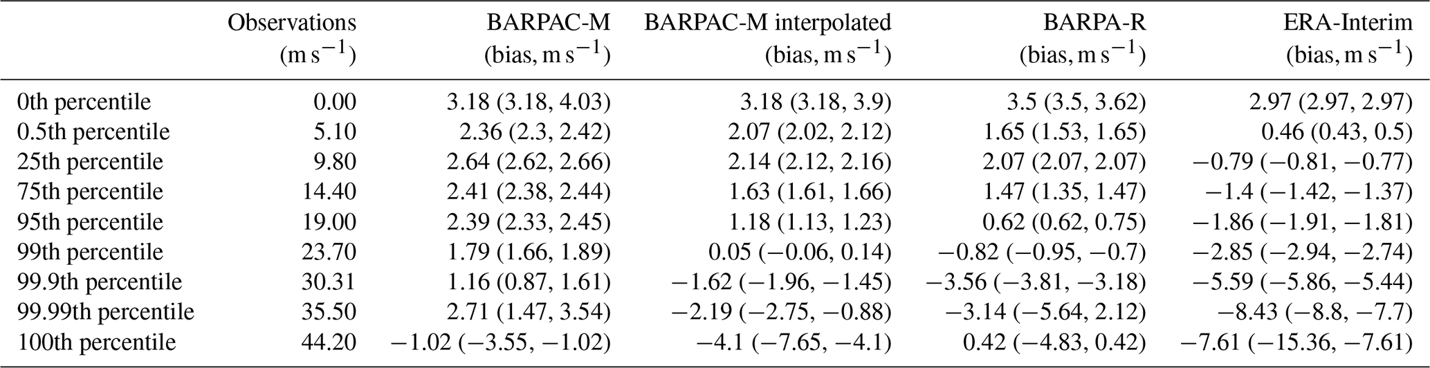
BARPAC-M is able to broadly reproduce the observed wind gust ratio distribution for severe (+25 m s⁻¹) daily maximum wind gusts, while BARPA-R produces much lower values of the wind gust ratio (Fig. 3). Note that the threshold of 25 m s⁻¹ for severe gusts is chosen for consistency with forecasting definitions (http://www.bom.gov.au/weather-services/severe-weather-knowledge-centre/severethunder.shtml, last access: 22 May 2023), with the number of daily maximum gusts that exceed 25 m s⁻¹ shown at the bottom of Fig. 3. This corresponds to around the 99th percentile based on the entire observational wind gust distribution (Table 1).

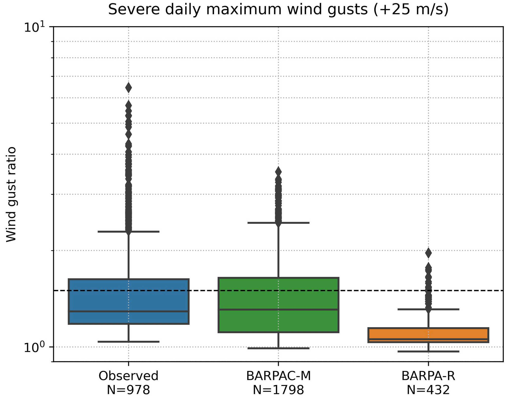
Figure 3 Boxplots indicating the distribution of wind gust ratios for severe daily maximum gusts from station observations, BARPAC-M hindcast, and BARPA-R hindcast. Boxes range from the 25th to the 75th percentile, horizontal lines represent the median, and whiskers represent 1.5 times the inter-quartile range. A dashed black line indicates a wind gust ratio of 1.5, and the total number of severe gusts (N) is indicated beneath each boxplot. Note that a logarithmic scale is used on the vertical axis.

A wind gust ratio threshold of 1.5 will be used here to classify a wind gust as convective. This value is consistent with the value used by Durañona et al. (2007) for defining extreme non-synoptic wind gusts and similar to the value of 2 by El Rafei et al. (2023), noting that the 10 min maximum gust data used here would be expected to result in lower overall wind gust ratios compared with the 1 min maximum gust data used in that study. A wind gust ratio of 1.5 also appears to reasonably discriminate between lightning-associated daily maximum wind gusts and non-lightning-associated daily maximum wind gusts (Sect. S4). This threshold is exceeded by around 31 % of severe daily maximum gusts in observations and 34 % of severe gusts in BARPAC-M but is only exceeded by 3 % of severe gusts in BARPA-R. This is expected given that the BARPA-R model configuration does not have an explicit representation of convective processes, with severe gusts in that model likely driven by larger-scale processes that persist over several hours.

For the remainder of this paper, analyses of simulated and observed wind gusts associated with convection will use a wind gust ratio threshold of 1.5 applied to daily maximum wind gusts. Daily maximum gusts that exceed a wind gust ratio of 1.5 will be referred to as convective gusts and will be compared with non-convective gusts. By discriminating between two types of wind gusts and comparing each BARPA distribution with observations, improvements in the BARPAC-M extreme wind speed representation can clearly be attributed to the representation of convective gusts (Fig. 4). In contrast, the biases in non-convective gust speeds are very similar between BARPAC-M and BARPA-R.

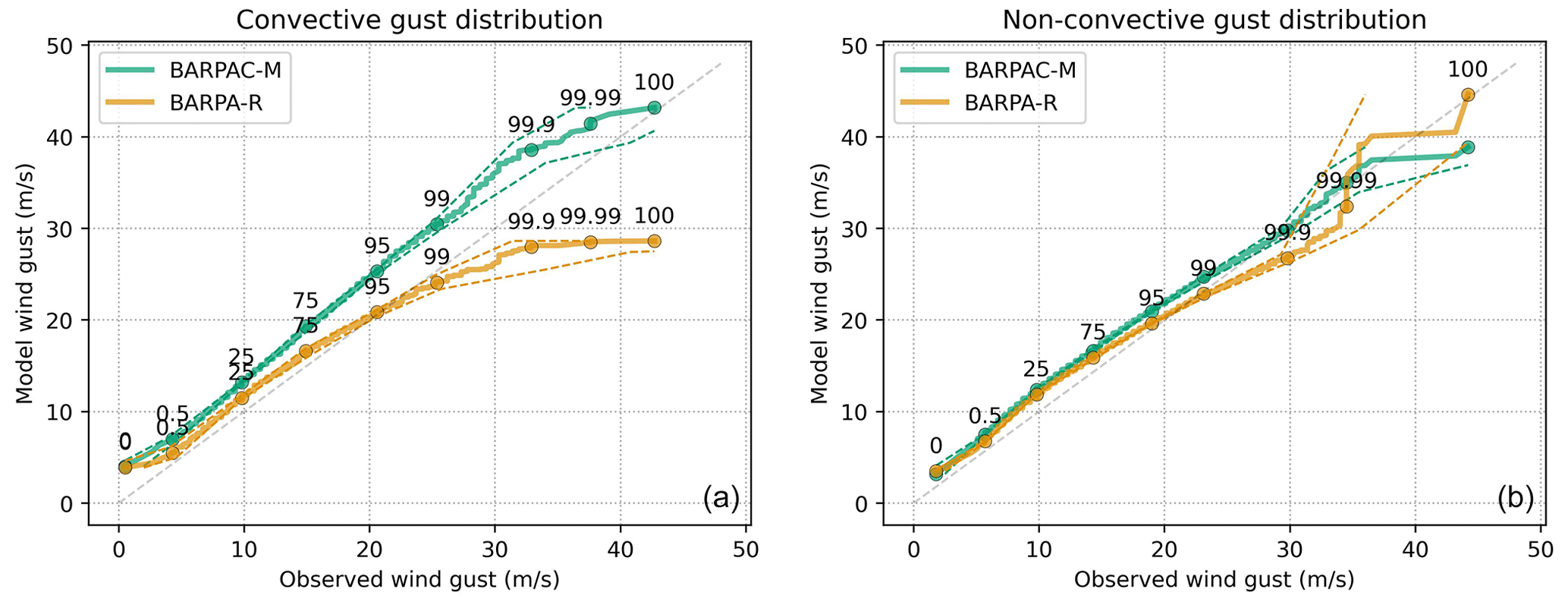
Figure 4 As in Fig. 2b and d but for (a) convective daily maximum wind gusts and (b) non-convective daily maximum wind gusts from BARPAC-M (green) and BARPA-R (orange). Convective and non-convective gusts are defined by a wind gust ratio threshold of 1.5.

Manual checks of two individual severe convective wind events produced by the BARPAC-M hindcast show that the model has physically realistic behaviour compared with analogous events based on observations (see Sect. S5). This includes spatial wind gust structures that might be expected in reality based on observed reflectivity structures and simulated wind gust time series that appear similar to the evolution of analogous measured gusts. This gives confidence in the ability of BARPAC-M to represent severe wind gusts associated with convection, in addition to the statistical approach presented in this section.

3.3 Different types of severe convective wind events

Here, we compare characteristics of SCWs in the BARPAC-M hindcast with observations, separately for different types of SCW events. Characteristics include the wind gust ratio, the ratio of the wind gust to the 0–6 km mean wind speed (“deep-layer wind ratio”), wind gust intensity, daily lightning counts, and spatial variability in SCW occurrence frequency across station locations. For the deep-layer wind ratio, the 0–6 km mean wind speed is calculated from ERA5 for observed events and from BARPA-R for the BARPAC-M events. High values of the deep-layer wind ratio represent gusts that are stronger than the background wind flow, indicating that those gusts are generated by internal storm processes, rather than by vertical mixing of strong synoptic winds due to convection, for example. A 0–6 km layer is chosen, as this is likely representative of the background flow relevant for vertical mixing by downdraughts and storm motion, with wind speed data over this layer already available based on their application for event clustering (see Sect. S2).

The separation of different event types is important given that there are a range of physical processes that can lead to severe surface winds associated with convection (e.g. Wakimoto, 2001) and the extent to which these processes are represented by BARPAC-M may vary. Three event types are defined here, based on clustering developed by Brown et al. (2023), that depend on the large-scale environment (see Sect. S2 for more details). This clustering results in SCW events with strong background wind, steep lapse rates, and high moisture. Brown et al. (2023) suggest that events with strong background wind are related to the vertical transport of strong synoptic-scale winds by relatively shallow convection to the surface, while events with steep lapse rates appear to be driven by downdraughts associated with the evaporation and melting of precipitation in convective clouds and events with high moisture appear to be associated with the outflow of intense deep moist convection, including supercells. Environmental diagnostics for clustering are calculated using ERA5 for measured events, as well as BARPA-R for BARPAC-M events, using methods described in Sect. 2.

Consistent with Brown et al. (2023), Fig. 5c, e, and g demonstrate that the observed wind gust ratio, daily lightning flashes, and deep-layer wind ratio all increase with clusters that are supportive of relatively deep convection. That is, these quantities are highest for SCW events in the cluster with high moisture, followed by the clusters with steep lapse rates and strong background wind. BARPAC-M is able to replicate this behaviour for the distribution of daily lightning flashes (Fig. 5f) and the deep-layer wind ratio (Fig. 5h). This broad separation of SCW characteristics between different types of events gives some confidence in the suitability of applying the clustering method to BARPAC-M. In addition, the distribution of large-scale environmental diagnostics is broadly consistent between observations and BARPAC-M across event types, as shown in the Supplement (Sect. S2). However, there are also some key differences in SCW characteristics between BARPAC-M and the observed dataset for different event types. For example, while BARPAC-M produces higher wind gust ratios for SCWs associated with the cluster with steep lapse rates compared with the cluster with strong background wind, as observed (Fig. 5d), the model produces significantly lower values for the cluster with high moisture compared with observations. This suggests that key processes related to SCWs within the cluster with high moisture are not represented in BARPAC-M. This could relate to, for example, supercell downdraughts that occur on small spatial scales and mostly occur within this cluster (Brown et al., 2023). There appears to be little difference in the severe wind gust intensity distribution between clusters, based on the results here (Fig. 5a–b).

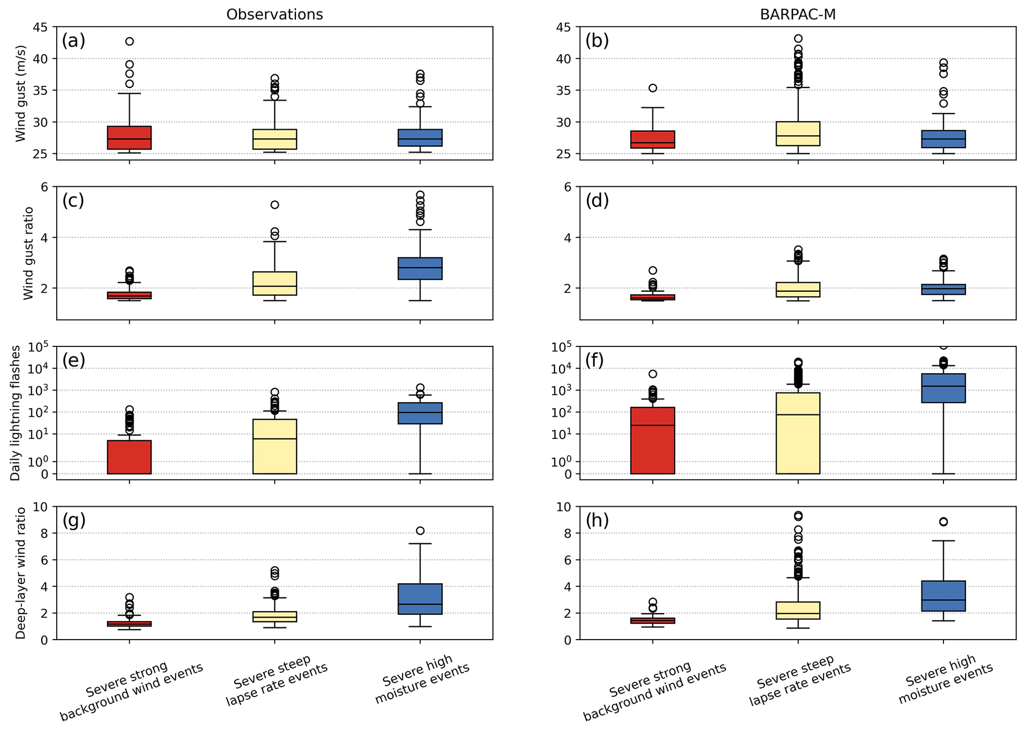
Figure 5 Boxplot distributions showing the distributions of the (a, b) wind gust speed, (c, d) wind gust ratio, (e, f) daily lightning flashes, and (g, h) deep-layer wind ratio, for severe convective daily maximum wind gusts from (a, c, e, g) station observations and (b, d, f, h) the BARPAC-M hindcast. Distributions are shown separately for severe convective daily maximum wind gusts that are associated with environments with strong background wind (red boxes), steep lapse rates (yellow boxes), and high moisture (blue boxes). Boxes range from the 25th to 75th percentile, and whiskers show 1.5 times the inter-quartile range, with circles representing data outside this range.

BARPAC-M also appears to broadly reproduce the observed spatial variability in SCW event occurrence frequency between different environmental clusters (Fig. 6). This includes events with strong background wind mostly occurring in the south of the domain, events with steep lapse rates occurring at a wide range of locations including inland, and events with high moisture occurring mostly in the coastal and eastern part of the domain. Figure 6 also shows that the total number of events between BARPAC-M and observations is comparable for the cluster with strong background wind (100 and 89 from observations and BARPAC-M, respectively) and cluster with high moisture (99 and 124), although the number of events with steep lapse rates is significantly overestimated (100 and 401).

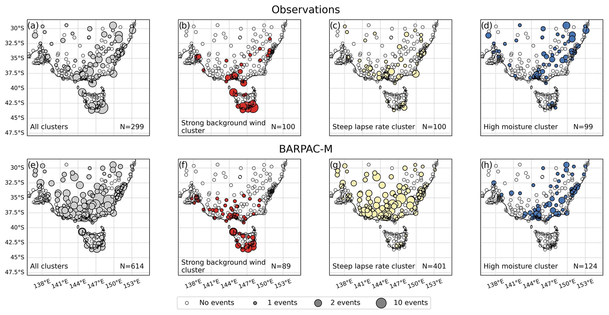
Figure 6 Maps showing the relative number of severe convective daily maximum wind gusts at each AWS location, with the size of the circle location markers scaled by event occurrences based on (a–d) station observations and (e–h) the BARPAC-M hindcast. Maps are shown separately for (a, e) all environments, (b, f) environments with strong background wind, (c, g) environments with steep lapse rates, and (d, h) environments with high moisture. The total number of events shown on each map is indicated on the bottom right of each panel. Empty circles represent stations with no events.

This bias in the number of BARPAC-M SCW events is investigated further here using quantile–quantile plots comparing the daily maximum wind gust distribution between BARPAC-M and observations for each environmental cluster, separately for all convective and non-convective gusts (Fig. 7). Results indicate that BARPAC-M tends to overestimate the intensity distribution of convective daily maximum wind gusts (Fig. 7d–f), especially when considering severe gusts over 25 m s⁻¹ in the cluster with steep lapse rates (Fig. 7e). This bias results in a greater portion of the BARPAC-M convective wind gust distribution exceeding the 25 m s⁻¹ severe threshold in environments with steep lapse rates, compared with observations, and therefore relates to the overestimation of simulated SCW events with steep lapse rates presented earlier (Fig. 6c and g) and in the overall number of SCW events (Fig. 6a and e). These errors appear to be greatly reduced for non-convective daily maximum wind gusts but with a slight high bias (Fig. 7a–c).

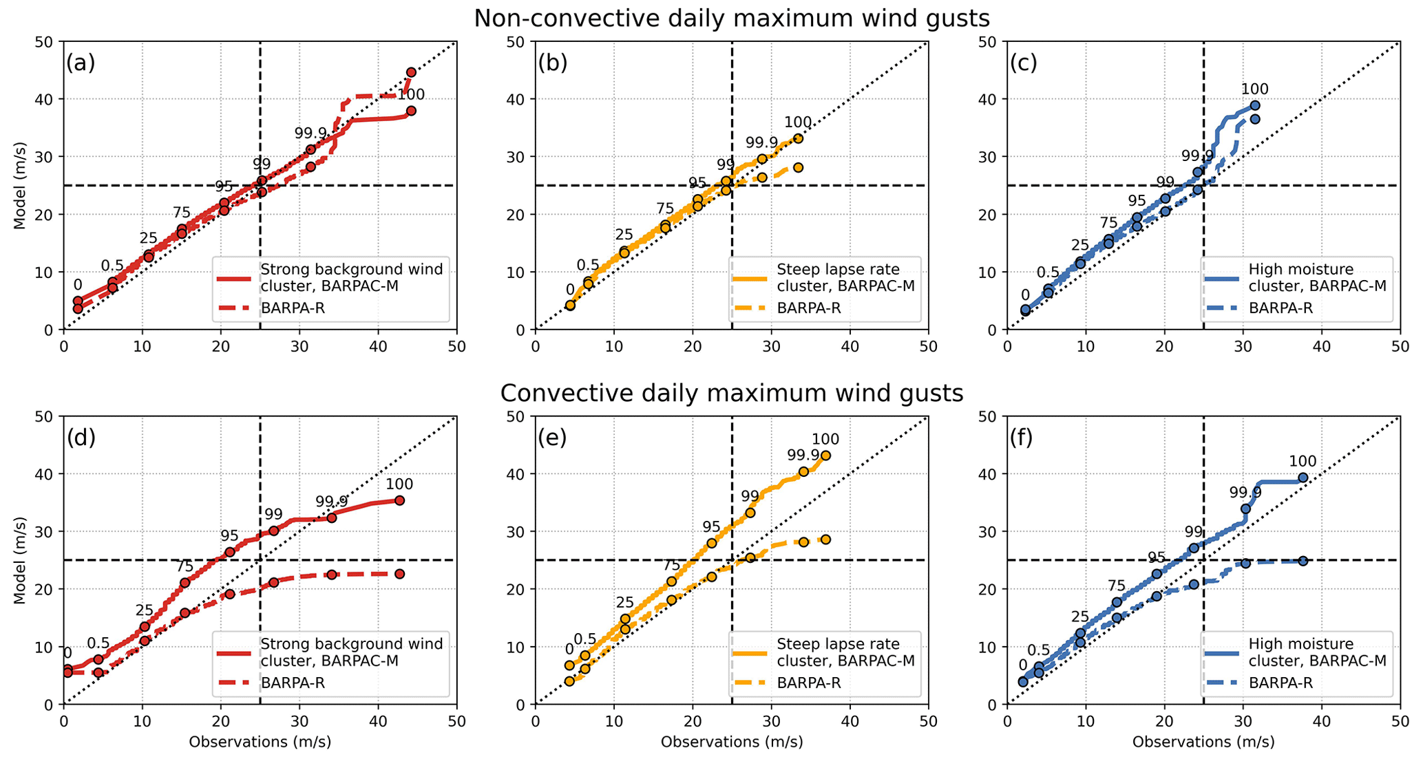
Figure 7 Quantile–quantile plots comparing the distribution of daily maximum (a–c) convective gusts and (d–f) non-convective gusts from station observations and the BARPAC-M hindcast. Shown for three different environmental clusters: (a, d) strong background wind, (b, e) steep lapse rates, and (c, f) high moisture. Bold dashed lines indicate the threshold used to define severe events. BARPA-R distributions are also shown in a dotted line, for reference. The number of quantiles used for plotting and the labelled percentiles are the same as in Fig. 2.

This overestimation in the number of SCW events with steep lapse rates could be due to several factors. These include biases in the large-scale environment inherited from BARPA-R, with a slightly higher occurrence frequency of favourable environments with steep lapse rates compared with ERA5 (see Fig. S8b). However, the relative bias in favourable environments with steep lapse rates is much smaller than the relative bias in simulated SCW event frequency from BARPAC-M within environments with steep lapse rates (compare Fig. S8b and c). This suggests that the bias in simulated SCW event frequency is not primarily driven by biases from BARPA-R and is instead due to errors in dynamical processes related to SCWs in BARPAC-M, such as convective downdraughts that are too intense or numerous or errors in gust parameterisations (explored further in the Discussion section). This is further supported by a relatively consistent frequency in daily lightning occurrence between BARPAC-M and WWLLN for environments with steep lapse rates, compared with the frequency of SCW occurrence (see Fig. S8d).

4 Future changes in severe convective wind events

Firstly, we compare the entire distribution of daily maximum convective wind gust speeds between historical and mid-century BARPAC-M simulations, forced by the ACCESS1-0 climate model (see Sect. 2.1). This is done using daily maximum convective wind gusts from the entire model domain, using land points only. According to the results shown in Fig. 8, BARPAC-M suggests an upwards shift in the daily maximum convective wind gust distribution for the extreme upper tail (over 40 m s⁻¹), consistent with Dowdy et al. (2021), who also analyse future BARPAC-M wind gust changes (their Fig. 4.4c). However, resampling different years in each simulation indicates high levels of uncertainty, with the future wind gust distribution potentially not being significantly different from the historical distribution (confidence interval shown by dashed lines in the Fig. 8b quantile–quantile plot). Some of this uncertainty is due to extreme gusts that are in some cases related to the same convective systems (or neighbouring convective systems). This uncertainty is supported by spatial wind gust intensity changes for the extreme upper tail that have no coherent spatial structure (see 20-year maximum wind gust changes in Sect. S7). The spatial changes likely relate to individual convective storm tracks and result in a low signal-to-noise ratio. The above points highlight the challenge of assessing future potential changes in the intensity of convective phenomena.

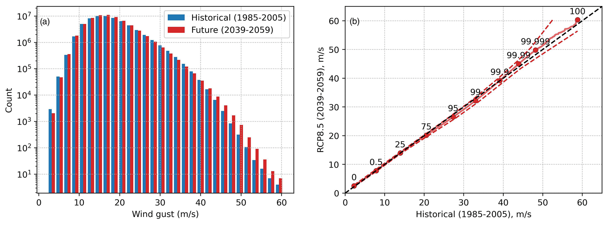
Figure 8 (a) Histograms comparing the December–February daily maximum convective wind gust distribution between the historical and RCP8.5 mid-century BARPAC-M simulations, over the entire BARPAC-M domain. (b) Quantile–quantile plot as in Fig. 2 but comparing the historical and mid-century convective wind gust distributions, with dashed lines representing a 95 % confidence interval calculated by randomly resampling different years from the future BARPAC-M simulation 1000 times with replacement. The dashed diagonal line represents a theoretical plot if both distributions were identical.

We now investigate future changes in the frequency of SCWs, defined by a wind gust threshold of 25 m s⁻¹ and wind gust ratio of 1.5. This is done by calculating the mean daily occurrence probability of simulated SCW events in historical and mid-century BARPAC-M climate simulations, across all spatial (land) grid points. Changes in simulated SCWs will be analysed for each of the event types presented in Sect. 3.3, with event clustering performed using BARPA-R data. Future changes in simulated SCWs are also compared to changes in the mean daily occurrence probability of a favourable SCW environment from BARPA-R (F_ENV), using the method of Brown and Dowdy (2021a), as described in Sect. 2.3. For comparison here, BARPAC-M-simulated SCWs are regridded to the BARPA-R grid by taking a maximum of one simulated SCW occurrence within each BARPA-R grid cell.

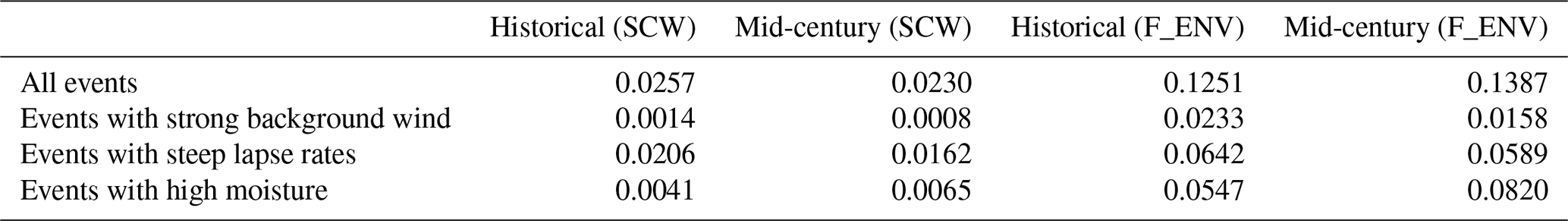
BARPAC-M suggests a decrease in the mean daily occurrence probability of simulated SCWs in the mid-century climate scenario, relative to the historical scenario (Fig. 9a), equivalent to a −10.5 % change. This decrease is primarily due to decreases in the occurrence probability of events with steep lapse rates, given the relatively high base probability of events with steep lapse rates compared with other clusters (Table 2, Fig. 6). However, it should be noted that there is a bias for BARPAC-M to produce an unrealistically high number of SCWs in environments with steep lapse rates, based on comparisons with observed event frequency (Sect. 3.3), and this result should be therefore treated with caution. Figure 9a also shows small decreases in simulated SCW probabilities within the cluster with strong background wind, while increases are shown for the cluster with high moisture. Due to large variability in event occurrences (see spatial maps of change in Sect. S7), total changes are not statistically distinct from zero, although cluster-wise results are less uncertain (95 % uncertainty range based on random resampling of different years is shown in Fig. 9a). These cluster-wise future changes are similar when considering changes in SCW probability conditional on the occurrence of each cluster (hatched bars in Fig. 9a), although the change in conditional occurrence probability for the cluster with steep lapse rates may not be statistically distinct from zero, due to the large variability noted previously.

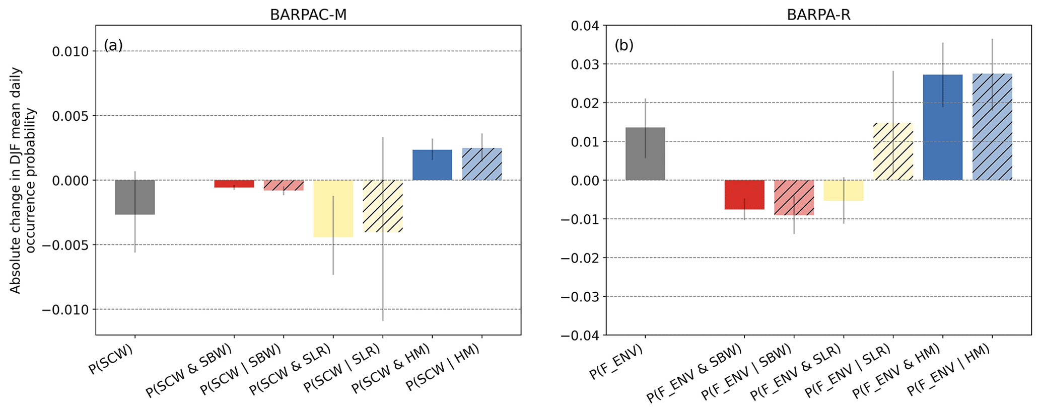
Figure 9 (a) Change in mean December–February (DJF) daily occurrence probability of a simulated severe convective wind (SCW) event, from BARPAC-M, between the historical and mid-century climate simulations. (b) Change in mean daily occurrence probability of a favourable severe convective wind environment (F_ENV), from BARPA-R. Shown separately for environments with strong background wind (SBW, red), steep lapse rates (SLR, yellow), and high moisture (HM, blue), as well as for all events (grey). For individual clusters, two probabilities are shown: the absolute change in the probability of occurrence considering all days (in solid bars, P(SCW & SBW), for example), and the probability conditional on that environmental cluster occurring (in hatched bars, P(SCW|SBW), for example). A two-sided 95 % confidence interval is shown with grey lines, estimated by randomly resampling years from the future period 1000 times with replacement.

Table 2 Mean daily occurrence probability of simulated severe convective wind events from BARPAC-M (SCW) and favourable SCW environments from BARPA-R (F_ENV) for each environmental cluster and all clusters combined. Shown separately for the historical and mid-century climate simulations.

In contrast to overall decreases in SCW probability shown by BARPAC-M, BARPA-R suggests future increases in the mean daily occurrence probability of favourable SCW environments (F_ENVs; see Fig. 9b) equivalent to an increase of 10.9 %. Although changes in F_ENV for each environmental cluster are the same sign as the changes in simulated SCWs from BARPAC-M, there is a higher increase in the F_ENV probability of the cluster with high moisture relative to other clusters and a smaller relative decrease in the F_ENV probability of the cluster with steep lapse rates. This leads to an overall increase in F_ENVs. Considering conditional probabilities, results for the cluster with strong background wind and high moisture are the same as for the non-conditional probabilities. However, there is an increase in the probability of a favourable environment with steep lapse rates conditional on the occurrence of that cluster, compared with a decrease in the non-conditional probability. This indicates that although there is a decrease in the number of environments with steep lapse rates, these are more favourable for SCWs when they do occur. However, the opposite is true for the conditional probability of simulated BARPAC-M SCWs in environments with steep lapse rates, noting large uncertainties (Fig. 9a).

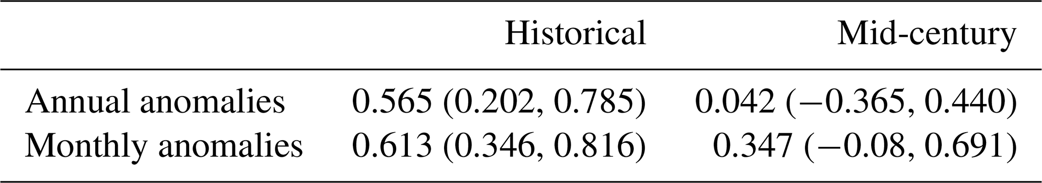
Because there is an overall decrease in SCW probability and an overall increase in F_ENV probability as discussed above, the relationship between the annual number of simulated SCWs and F_ENVs is less correlated in the future period relative to the historical period (Table 3). The relationship based on monthly anomalies also becomes weaker but to a lesser extent compared with the annual anomalies. The weakening of this relationship potentially highlights the limitation of applying environmental diagnostics to future projections, given that other factors influencing the formation of severe convection could change in the future, as noted by previous studies (for example Hoogewind et al., 2017).

Table 3 Pearson correlation coefficients describing the relationship between the mean annual and monthly anomalies of December–February simulated severe convective wind occurrence from BARPAC-M and the anomalies of favourable environment occurrences from BARPA-R. Shown separately for the historical and mid-century climate scenarios. A 95 % confidence interval is indicated in brackets, calculated by randomly resampling the annual and monthly time series 1000 times with replacement.

5 Discussion

A convection-permitting configuration of the BARPA modelling framework with 2.2 km horizontal grid spacing (BARPAC-M) shows significant improvements over a 12 km BARPA configuration (BARPA-R) and a global reanalysis that provides atmospheric forcing (ERA-Interim) in representing the extreme upper tail of the observed daily maximum wind gust distribution over 11 December–February periods. These improvements shown here seem to be due to a combination of higher spatial resolution in BARPAC-M output and enhanced representation of severe wind gusts related to convective processes that are not represented explicitly in coarse-scale models. Findings shown here for extreme winds including severe convective winds (SCWs) in eastern Australia are consistent with numerous studies that have demonstrated the potential added value from convection-permitting models over coarse-scale models, related to convective storm forecasting (e.g. Done et al., 2004; Clark et al., 2009) and the representation of extreme sub-daily precipitation (see reviews by Prein, 2015; Kendon et al., 2021) and extreme wind climates (Manning et al., 2022; Belušić Vozila et al., 2023).

However, BARPAC-M still has significant biases related to the representation of the extreme regional wind climate. This includes an overestimation of SCW event frequency based on the occurrence of convective gusts of at least 25 m s⁻¹, particularly in environments with steep lapse rates where event frequency is overestimated by a factor of 4. This could potentially be related to biases in the parameterisation of turbulent gusts at the surface, which depends on temporal fluctuations in the resolved wind and the surface layer stability profile and/or the representation of convective processes and storm-scale dynamics. For example, El Rafei et al. (2023) found a systematic positive bias in the turbulent gust representation of a reanalysis version of BARPAC-M run at 1.5 km grid spacing with data assimilation over subtropical eastern Australia. In addition, bias for too many intense convective cells has been shown previously for the Unified Model (that BARPA is based on) compared with radar observations in the United Kingdom (Hanley et al., 2015) and in tropical Australia (Jucker et al., 2020; Bergemann et al., 2022) and is consistent with the results here for SCW frequency. Unfortunately, we are unable to determine further details regarding the convection and storm dynamics in BARPAC-M here due to a lack of available data, although this should be a focus of future work.

With these biases in mind, future simulated changes in SCW event probability are analysed from a mid-century RCP8.5 BARPAC-M climate simulation and compared with changes in favourable SCW environments from the regional BARPA-R model. This comparison is intended to provide insights into the consistency between two commonly used methods for future climate projections of convective hazards. In addition, future changes are compared separately for three types of SCW events that have been shown to occur in this region, based on statistical clustering of the large-scale environment (Brown et al., 2023). A future projected increase in environments with high moisture favourable for SCWs is suggested by BARPA-R. These types of favourable environments are often associated with high amounts of CAPE (convective available potential energy; Brown et al., 2023), and so these future changes agree with previous studies that determine hazardous convective environments from GCMs using CAPE-based diagnostics (for example, Allen et al., 2014; Seeley and Romps, 2015; Lepore et al., 2021). In contrast, favourable environments with steep lapse rates, which are likely associated with dry microburst processes (Brown et al., 2023), are projected to decrease in frequency. This supports the findings of Brown and Dowdy (2021a), who showed that the frequency of favourable SCW environments decreases under an end-of-century RCP8.5 scenario when applying environmental proxies based on temperature lapse rates, compared with an increase when using proxies based on CAPE. In addition, favourable environments with strong background wind, which are associated with low CAPE and high amounts of vertical wind shear (Sherburn and Parker, 2014; Brown et al., 2023), are also projected to decrease in frequency. Similar to previous studies in other regions such as Hoogewind et al. (2017) and Haberlie et al. (2022), the BARPAC-M convection-permitting model indicates future changes that are the same sign as the environmental changes from the driving model, within each type of environment. However, because the majority of BARPAC-M events occur in environments with steep lapse rates, the overall future change suggested by that model is a decrease in simulated SCW frequency, while the opposite is true for the BARPA-R environmental method where environments with high moisture are relatively important. This indicates that considering different types of events is critical for understanding future projections of SCWs in this region. This also highlights that process-based biases in the frequency of simulated events could potentially have an impact on future projections, such as an unrealistically high number of events with steep lapse rates in BARPAC-M, and that these projections should be treated with caution.

The annual and monthly (December–February) correlation between the number of favourable SCW environments (from BARPA-R) and simulated SCWs (from BARPAC-M) across the entire domain has also been investigated in the historical and future climate periods. In the historical period, an annual Pearson correlation of r=0.565 is reported with a monthly correlation of r=0.613. This is of a similar magnitude to the correlation between annual SCW environments and measured SCW events around Australia reported by Brown and Dowdy (2021a) (r=0.454) and between annual tornado reports and favourable environments in the United States documented by Gensini and Brooks (2018) (r=0.66) but lower than the relationship between monthly mean simulated hazardous convection (strong simulated updraughts) and favourable environments reported for the United States by Hoogewind et al. (2017) (r=0.91). In the future climate, a much weaker annual (r=0.042) and monthly (r=0.347) correlation between favourable SCW environments and simulated SCWs is reported here, due to the different future changes in favourable environments and simulated SCWs discussed above. This is in contrast to Hoogewind et al. (2017), who found that this correlation was equally strong in a future climate scenario (r=0.93). The lack of correlation between future simulated SCWs and favourable SCW environments found here highlights potential uncertainties in the application of methods that have been developed in the historical climate, as also mentioned by previous studies (Hoogewind et al., 2017; Raupach et al., 2021). This includes the application of the Brown and Dowdy (2021b) statistical diagnostic (BDSD) that is used here to diagnose favourable SCW environments (see Sect. 2.3). Additional uncertainty is also potentially introduced here by the fact that the BDSD was initially trained on an observational dataset (Brown and Dowdy, 2021b) and is being applied here to a regional climate model with a potentially different relationship between SCW events and the large-scale environment. Future work could be aimed at further investigating the physical mechanisms relating favourable SCW environments to simulated events in current and future climates. Although the future changes reported here have low confidence based on this discussion, our results suggest a potential increase in the frequency of SCWs in environments with high moisture, which may be compensated by a reduction in SCWs in environments with steep lapse rates.

A potential benefit of convection-permitting climate modelling is that simulated changes in the intensity of convective hazards are able to be analysed, compared with environmental approaches that are generally limited to changes in occurrence frequency. Future changes in extreme convective wind gust speeds are relevant for design and adaptation (Holmes, 2002; Lombardo and Zickar, 2020) and have therefore been analysed here using BARPAC-M for southeastern Australia. Although the mid-century BARPAC-M scenario does suggest increases in the occurrence of daily maximum convective gusts that exceed 40 m s⁻¹, these changes are not statistically significant based on random resampling of different years. This is due to the high amounts of spatial and temporal variability in these convective-scale events, including many events occurring on a single day in the future period, for example. This demonstrates the challenges of assessing future changes in simulated convective hazards for relatively rare events, such as gusts exceeding 40 m s⁻¹. The approach used in this study could be complemented by future work using idealised and/or realistic modelling of projected future individual events, similar to work already underway using pseudo-global-warming approaches (González-Alemán et al., 2023; Li et al., 2023).

The uncertainties related to extreme wind events mentioned above could also be associated with internal climate variability, including natural modes of variability such as the El Niño–Southern Oscillation (ENSO) and others, which could potentially affect the future projections presented here more generally. Internal variability can be a source of uncertainties in future climate projections (Deser et al., 2012) as well as in historical trends of severe thunderstorm environments for this region (Allen and Karoly, 2014). Uncertainties from internal variability could be exacerbated by the relatively short 20-year period used for the analysis here, noting that this was the maximum period of data available for use and that these data were used in previous research such as described in Dowdy et al. (2021). Simulating long periods with convection-permitting models is very computationally demanding, as noted by previous studies that have used temporal windows with a length of about 10–15 years for future projections of severe convection (Gensini and Mote, 2015; Ashley et al., 2023). Future work to provide convection-permitting climate model simulations over longer periods will be beneficial, including with a larger sample helping to reduce the influence of internal climate variability (associated with ENSO, for example) on estimates of longer-term climate changes. In addition, the relationships between SCW events and individual modes of climate variability in this region are relatively uncertain, with conflicting results for severe convection based on lightning and hail observations and severe thunderstorm environments (Allen and Karoly, 2014; Dowdy, 2016; Soderholm et al., 2017; Dowdy, 2020). Future work towards revealing these relationships could likely provide additional insights into the potential impact of internal climate variability on historical and future trends in convective hazards, including severe wind gusts.

6 Conclusions

Here, the wind gust intensity distribution from a convection-permitting model hindcast (BARPAC-M) has been evaluated using an observational dataset and compared with distributions from the associated forcing models. Daily maximum wind gusts are assessed during December–February in southeastern Australia, over an 11-year period. The characteristics of severe gusts associated with convection, as represented by the convection-permitting model, have been compared and contrasted with observed characteristics. This is done for different types of SCW events, as diagnosed by statistical clustering applied to the large-scale environment. Severe convective wind (SCW) event occurrences are then compared between a historical and mid-century climate simulation using BARPAC-M, and future changes in simulated events are compared with changes in environmental conditions that are favourable for SCWs from the regional model that forces BARPAC-M (BARPA-R). Key findings are as follows:

• BARPAC-M shows significant improvements in representing the extreme upper tail (above the 99th percentile) of the observed daily maximum wind gust intensity distribution compared with BARPA-R. Both of these models show improvements over the global forcing model, ERA-Interim, above the 75th percentile.

• Consistent with observations, BARPAC-M is shown to represent severe, transient wind gusts with high wind gust ratios. These gusts are likely related to deep convection and associated outflow and are not represented by BARPA-R, which parameterises convective processes.

• BARPAC-M can replicate some of the variability in wind gust characteristics and spatial patterns of occurrences between different types of severe convective wind events. However, some key processes appear to not be represented, as evidenced for example by lower wind gust ratios than observed for events in environments with high moisture.

• BARPAC-M tends to overestimate the frequency of severe convective wind gusts, particularly in environments with steep lapse rates. Based on findings from previous studies, this bias is likely due to a combination of errors in the surface wind gust parameterisation for convective outflow, as well as in the frequency and/or intensity of deep convection.

• BARPAC-M indicates a decrease in the occurrence of simulated severe convective wind events under a mid-century RCP8.5 scenario, driven by a decrease in events within environments with steep lapse rates. However, this result is uncertain due to large variability in event occurrences and model biases, as are future estimated changes in convective wind gust intensity.

• In contrast, an overall future increase in the frequency of favourable SCW environments is suggested, driven by an increase in favourable environments with high moisture. As a result, the relationship between the annual and monthly number of simulated severe convective wind events and favourable environments is less correlated in the mid-century scenario compared with the historical simulation.

These findings are intended to provide insight into future regional projections in the frequency and intensity of severe wind gusts associated with convection. Future work should continue to evaluate convection-permitting models and their representation of convective hazards, with an emphasis on physical processes. In addition, experiments using forcings from a range of future climate scenarios should provide important information for projections of severe convective hazards, including an estimation of scenario uncertainty that has not been investigated here. Results show that BARPAC-M appears somewhat suitable in the application of future wind projections, based on the ability to reliably represent the extreme tail of the distribution of daily maximum wind gusts and SCW characteristics aggregated over a large number of events. However, the overestimation of simulated events in environments with steep lapse rates strongly influences the future changes indicated by the model. This change disagrees with estimates based on environmental changes and represents a significant uncertainty. This suggests that future projections for convective hazards such as SCWs should be done using a multi-model approach to account for uncertainties in the representation of convective processes.