Global estimates of 100-year return values of daily precipitation from ensemble weather prediction data

High-impact river floods are often caused by very extreme precipitation events with return periods of several decades or centuries, and the design of flood protection measures thus relies on reliable estimates of the corresponding return values. However, calculating such return values from observations is associated with large statistical uncertainties due to the limited length of observational time series, uneven spatial distributions of rain gauges and trends associated with anthropogenic climate change. Here, 100-year return values of daily precipitation are estimated on a global grid based on a large data set of model-generated precipitation events from ensemble weather prediction. In this way, the statistical uncertainties in the return values can be substantially reduced compared to observational estimates due to the substantially longer time series. In spite of a general agreement in spatial patterns, the model-generated data set leads to systematically higher return values than the observations in many regions, with statistically significant differences, for instance, over the Amazon, western Africa, the Arabian Peninsula and India. This might be linked to an overestimation of tropical extreme precipitation in the model or an underestimation of extreme precipitation events in observations, which, if true, would have important consequences for practical water management.

1 Introduction

Extreme precipitation is often associated with river floods, which are one of the most dangerous hazards for society and have caused high socioeconomic losses around the globe (Merz et al., 2021; Kron, 2015; Barredo, 2007; Douben, 2006). There are many historical examples of these events such as several flash floods due to a mesoscale convective system in South America in 2022 (Alcântara et al., 2023), an extreme flood event in central Europe in 2021 (Mohr et al., 2023) and widespread flooding in Thailand during the monsoon season in 2011 (Gale and Saunders, 2013). River floods typically develop along one of two distinct pathways: either very quickly in the form of a flash flood or as a slower increase in the runoff and water levels over several hours. On the one hand, flash floods, which often occur in smaller rivers, are associated with very high precipitation rates in a spatially limited domain, leading to quickly developing peak discharge (Sene, 2016) that can threaten society along the river route and also downstream of the extreme precipitation event. On the other hand, larger-scale floods in larger rivers with a slower increase in water levels are typically caused by longer-lasting heavy precipitation over a larger area. A multitude of atmospheric drivers can contribute to the development of such extreme precipitation events and floods in different regions around the globe, such as convective cells, mesoscale convective systems, monsoonal lows, or intense upper-level troughs or cut-off lows (Alcântara et al., 2023; Mohr et al., 2023; Ruff and Pfahl, 2023; Gaume et al., 2016; Gale and Saunders, 2013). In addition, orographic enhancement of precipitation can contribute to the development of floods in complex terrain.

The increase in global population, especially in high-risk areas, and the rise in the vulnerability of society increases the risk of flood disasters (Kron, 2015). Moreover, climate simulations project that the frequency and intensity of extreme precipitation events is going to increase in a warmer climate (Pendergrass and Hartmann, 2014; Fischer et al., 2013; O'Gorman and Schneider, 2009), which is also associated with increasing frequency of intense floods (see e.g. Alfieri et al., 2015). This, along with higher exposure of a growing proportion of the population to floods in a warmer climate, will drastically increase the flood risk on a global scale (Tellman et al., 2021; Alfieri et al., 2017; Jongman et al., 2012). In order to reduce or even prevent flood losses and damage, different kinds of flood protection measures have been developed. More-recent extreme events have shown that flood damage has been reduced with the help of flood barriers, compared to damage from extreme precipitation that occurred several decades ago (see e.g. Merz et al., 2014; Bissolli et al., 2011), and that there is further potential to minimise flood losses in the future (Jongman et al., 2015). To this end, e.g. for the appropriate construction of dikes, it is crucial to precisely determine the amount of precipitation from potential extreme events that the protection measures should be able to withstand. In practical water management, such an event is often denoted “probable maximum precipitation” (World Meteorological Organization, 2009).

From a statistical point of view, this probable maximum precipitation can be quantified as the precipitation amount associated with extreme events with long return periods, typically on the order of 100 years, through extreme value statistics. To estimate such return values, long precipitation time series are required, which are conventionally obtained from observations. Although there are several observational data sets available with high quality, relatively high temporal and spatial resolution, and coverage, this approach is affected by certain limitations (Rajulapati et al., 2020). First, the time series are often shorter than 100 years, which requires extrapolation to determine 100-year-or-larger return values and increases the associated statistical uncertainties. Second, in addition to the first limitation, there are different extreme value methods (type of distribution or parameter fitting) used to perform this extrapolation, which have to be selected by the users. Third, if global coverage is desired, the uneven spatial distribution of rain gauges requires combining different data sources (e.g. rain gauge and satellite data), which can lead to spatial inhomogeneity in the estimated return values and associated uncertainties. Combining different data sets with diverging representations of extreme precipitation can also lead to inconsistencies on local scales (see e.g. Rajulapati et al., 2020). And fourth, precipitation trends, e.g. due to anthropogenic climate change (Fischer et al., 2014), can compromise the extreme value statistics. Accordingly, Rajulapati et al. (2020) have shown that precipitation observations typically do not provide a consistent representation of extreme events and that 100-year return values differ significantly between observational data sets. Due to these limitations, previous studies often focused on extreme events with return periods of much less than 100 years (Rodrigues et al., 2020; Donat et al., 2013), for which observational time series are sufficient, and/or on specific regions (Rodrigues et al., 2020; Maraun et al., 2011). Alternatively, model simulations, for instance from weather prediction (Ruff and Pfahl, 2023), seasonal forecasts (Kelder et al., 2020) or climate models (Mizuta and Endo, 2020), can provide long time series that allow for a statistically robust estimate of 100-year return values as well. Nevertheless, these model-based estimates may of course suffer from other biases due to the imperfect representation of precipitation processes in the models.

In this study, we explore the possibility of using a model-generated data set from ensemble weather prediction for estimating 100-year return values of daily precipitation on a 1°×1° grid covering the entire globe, extending our previous analysis that focused on European river catchments (Ruff and Pfahl, 2023). The equivalent length of the weather prediction data set is about 1200 years, which is much longer than the 100-year return period, promoting statistical robustness. Due to the daily accumulation, relatively large spatial scale and limited model resolution, the studied extreme precipitation events are most relevant for larger-scale river floods and not as appropriate for local flash floods triggered by convective precipitation. The main goal of the study is to compare these model-based 100-year return values to estimates from three different observational data sets and quantify their relative biases and statistical uncertainties. This may provide a basis for using the model-generated data set also for practical estimates of probable maximum precipitation, in particular in data-sparse regions.

The following section describes the ensemble weather prediction data as well as three observational data sets that are applied to evaluate the differences between the model-based and observation-based estimates of 100-year return values. In Sect. 3, the statistical methods to evaluate the ensemble prediction data and determine return values and confidence intervals are explained in detail. The resulting return values, their confidence intervals and differences to observational data sets are presented in Sect. 4. Finally, conclusions and a discussion of the main findings and their limitations are provided in Sect. 5.

2 Data

The 100-year return values are estimated from a large global data set of daily precipitation events, which is obtained from ensemble weather prediction data. The resulting estimates are compared to observational data sets obtained from rain gauge measurements and satellites for evaluating the differences between a model-based and an observational approach. All data sets are described in the following sections.

2.1 Ensemble prediction data

In order to generate a large data set of realistic and daily precipitation events, ensemble weather prediction data are used. In this study, the ensemble prediction system (EPS) of the European Centre for Medium-Range Weather Forecasts (ECMWF) is accessed for this purpose. The ensemble predictions from the EPS are obtained from the Integrated Forecasting System (IFS), which is a comprehensive Earth system model with an atmospheric component from the ECMWF, and from other community models for certain other components of the Earth system (ECMWF, 2023f). More details regarding the IFS and the operational EPS forecasts are described in ECMWF (2023d). An operational weather prediction model is very useful for such an approach as the model is capable of representing daily precipitation events more realistically than, e.g. climate models, due to a comprehensive comparison to observations (even without a surface precipitation assimilation scheme). Nevertheless, the EPS data may suffer from interdependence between the ensemble members, which is investigated in more detail in Sect. 3.1, and from temporal inhomogeneities due to updates to the prediction system. The latter as well as additional limitations of the application of ensemble weather prediction data for the approach in this study are discussed in more detail in Sect. 5.

Started in March 2003, ensemble simulations of the operational weather prediction model are performed twice a day, at 00:00 and 12:00 UTC, with forecasting times of at least 10 d. The ensemble contains 51 ensemble members. One member is a controlled run without any perturbations, while the other 50 members represent runs with marginally changed initial conditions and with stochastic perturbations of the model physics. This results in 102 simulations per real day. More information about the workflow of the EPS can be found in Molteni et al. (1996).

The analyses in this study are based on daily precipitation sums, which are computed by adding up the large-scale and convective precipitation over 24 h. From each simulation, the daily precipitation sum of only the 10th forecast day (between forecast hours 216 and 240, the same procedure for every initialisation time) is selected instead of using all forecast days. This approach follows Ruff and Pfahl (2023), who used a daily precipitation data set from the EPS to investigate the atmospheric conditions during extreme precipitation events over central Europe, and Breivik et al. (2013), who estimated return values of oceanic surface wave heights from EPS data. The basis of the approach is the assumption that due to the advanced forecast time, the model realisation on the 10th forecast day does not significantly correlate with the conditions at the beginning of each specific simulation. In addition, an interdependence of consecutive days, which would also decrease the effective sample size of extreme events in further analyses, is excluded by selecting just 1 d of this multiday forecast. Therefore, the different realisations obtained from the ensemble members can be considered statistically independent from each other. While the simulations of individual ensemble members are highly correlated with each other in the beginning due to very similar initial conditions, this correlation reduces with increasing forecast time. This decrease is particularly large for precipitation compared to, e.g. geopotential height, due to its high variability in space and time and its dependence on small-scale processes. Both Ruff and Pfahl (2023) and Breivik et al. (2013) performed comprehensive statistical analyses to demonstrate the independence of the ensemble members on the 10th forecast day and to compare the statistics of daily precipitation and wave height to observational data. The data set used here is very similar to the data of Ruff and Pfahl (2023), except that they analysed spatially averaged precipitation time series over central European river catchments, while this study uses time series on a spatial grid of 1°×1° spanning the entire globe. Therefore, only a short statistical evaluation of the ensemble prediction data (see Sect. 3.1) adapted to time series at individual grid point is performed in this study, while we refer to Ruff and Pfahl (2023) for other, more detailed statistical analyses.

The operational model IFS has been updated on a regular basis. Certain technical and physical schemes have been changed with each implementation of a new model cycle during the years 2003–2019, in order to continuously improve the forecast skill. However, this has the potential to influence the simulated precipitation and the upcoming results of this study. Although mainly minor improvements were implemented within each individual model cycle, there are some important updates that include changed formulation of the humidity analysis (Cycle 26r1, in 2003), improved precipitation forecasts over Europe (Cycle 32r3, in 2007) and improved precipitation forecasts over coastal areas due to changes in cloud physics (Cycle 45r1, in 2018). Details of all model cycle changes are described in ECMWF (2023c), and a full documentation of each model cycle itself is available from ECMWF (2023d). Ruff and Pfahl (2023) have evaluated the influence of these model cycle updates on their daily precipitation time series. They demonstrated a systematic decrease in high precipitation percentiles (99th, 99.9th and 99.99th) that corresponds to extreme precipitation events with large return periods over central Europe within the first 5 years of the ensemble simulations (2003–2007). On the contrary, since 2008 the amplitude of these percentiles is rather constant, as discussed in more detail in Sect. 3.1. Hence, in order to avoid any temporal inconsistencies within the data set, only the ensemble simulations from 1 January 2008 until 31 December 2019 are used in this study, following Ruff and Pfahl (2023). The restricted time period of 12 years of forecasts from the EPS archive, along with 102 daily simulations, provides a data set with an equivalent length of 1224 years of modelled but realistic daily precipitation events. The data set is available on a regular lat–long grid with increasing resolutions over time (higher than 1°×1° over the entire period) due to changes in the forecast model cycles. For a consistent analysis and comparison to observational data, they are downloaded on a coarser grid (here 1°×1°). During that process, the Meteorological Interpolation and Regridding (MIR) scheme by the ECMWF “up-scales” the data by linear interpolation based on a triangular mesh, which is a drawback for the current study since it does not, in general, conserve area-mean precipitation. More details can be found in ECMWF (2023e, g).

2.2 Observational data sets

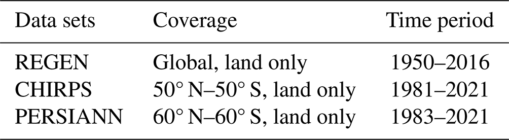
One observational data set based on rain gauge measurements from Rainfall Estimates on a Gridded Network (REGEN) and two data sets based on a combination of satellite data and rain gauges from Climate Hazards Group Infrared Precipitation with Stations (CHIRPS) and Precipitation Estimation from Remotely Sensed Information using Artificial Neural Networks–Climate Data Record (PERSIANN) are used to compare observations and daily 100-year precipitation return values and their confidence intervals from the EPS forecasts. The observational data sets mainly differ in their covered regions, the type and number of observations, and the interpolation of the data to a regular lat–long grid. The observational data sets are first regridded and then the very high return values are determined in order to provide extremes of area-averaged precipitation. This is relevant for large-scale precipitation extremes over large river catchments, on which this study focuses, and provides the best comparability to the model-generated EPS data. More detailed descriptions of the observations can be found in the following sections. The most important information for all observational data sets as used in this study is summarised in Table 1.

2.2.1 REGEN data

REGEN is an observational data set for daily precipitation that uses quality controlled rain gauge measurements, spatially interpolated from daily precipitation data of large observational archives such as the Global Historical Climate Network Daily provided by the National Oceanic and Atmospheric Administration and the Global Precipitation Climatology Centre provided by the Deutscher Wetterdienst. More information about this data set is presented in Contractor et al. (2020b). The spatial density of available rain gauges is very different between certain regions. Especially over Africa and central Asia, the rain gauge density is considerably lower than over North America, Europe and Australia. The reliability of these precipitation observations for specific regions can be evaluated with a quality mask, which takes, for instance, the weather station density and interpolation variation measures into account (Contractor et al., 2020b). Trustworthy areas are mainly located over North America, Europe and Australia, as well as over large parts of continental Asia, Brazil and South Africa. While this study only uses the daily precipitation sums (version 1-2019), other information is additionally available on a global grid such as, e.g. the number of rain gauges and the standard deviation of the precipitation sums. The precipitation data are constructed from around 135 000 rain gauges between 1 January 1950 and 31 December 2016. Not all stations are available for the entire period and the data can be used on a regular lat–long grid with a spatial resolution of 1°×1° for all global land areas except for Antarctica.

2.2.2 CHIRPS data

The CHIRPS data archive is a quasi-global daily precipitation data set hosted by the US Geological Survey Earth Resources Observation and Science Center in collaboration with the Santa Barbara Climate Hazards Group at the University of California. The CHIRPS data result from a combination of quasi-global geostationary thermal infrared satellite observations from two NOAA sources, in situ precipitation observations obtained from a variety of national and regional meteorological services, the Tropical Rainfall Measuring Mission product from NASA, a monthly precipitation climatology, and atmospheric model rainfall fields from the NOAA Climate Forecast System. A more-detailed description of the development workflow of the CHIRPS data can be found in Funk et al. (2014a). The data are available from 1 January 1981 until 31 December 2021 over land areas on a regular lat–long grid between 50° N and 50° S. In this study, the CHIRPS data (version 2.0) with a spatial resolution of 0.25°×0.25° are selected and averaged over a 1°×1° box for further analyses.

Table 1 Summary of the most important details of the REGEN, CHIRPS and PERSIANN observational data sets as used in this study.

2.2.3 PERSIANN data

The Precipitation Estimation from Remotely Sensed Information using Artificial Neural Networks–Climate Data Record (PERSIANN-CDR) hosted by the Center for Hydrometeorology and Remote Sensing at the University of California is a satellite based daily precipitation observation data set. This data set results from gridded satellite infrared data, obtained from a combination of several international geostationary satellites in combination with an artificial neural network training using hourly precipitation data from the National Centers for Environmental Prediction stage IV. Additionally, the monthly product of the Global Precipitation Climatology Project is used for bias adjustments. Further details on this data set are described in Ashouri et al. (2015b). The daily precipitation sums of this data set (version 1) are available from 1 January 1983 until 31 December 2021 on a regular lat–long grid between 60° N and 60° S with a spatial resolution of 0.25°×0.25°. In this study, the data are averaged over a 1°×1° box, and only data over land areas are used for further analyses. Missing values in the data set appear in cases when satellite data are not available and on dry days when no precipitation occurred (see Fig. S1 in the Supplement). As an under-representation of dry days strongly influences the evaluation of quantile distributions of the data (used for evaluations in Sect. 3.1), all missing values are set to 0 for further analyses in order to improve the representation of the percentiles. However, this also leads to errors over areas that are regularly affected by non-availability of satellite data. This is especially dominant at around 50° N and 70° E, which is why these areas should be taken into account when interpreting the results from the PERSIANN observations.

3 Methodology

In this section, statistical analyses of the suitability of the EPS data for determining 100-year precipitation return values on a global grid are presented. Subsequently, the method to determine the return values and their confidence intervals is described.

3.1 Statistical evaluation of the ensemble prediction data

For the determination of 100-year return values of daily precipitation on a global scale, the EPS data from the 10th forecast day are used as a large climatological data set. This implies that the data set can be considered a combination of realistic and independent realisations of daily precipitation in order to suitably apply extreme value statistics to this data set. Therefore, we evaluate if (1) the ensemble members can be considered independent from each other; (2) each ensemble member properly represents the statistical distribution of precipitation compared to observations; and (3) no significant trend in the high precipitation percentiles can be identified over time, following Ruff and Pfahl (2023) and Breivik et al. (2013). These criteria are statistically evaluated and discussed in the following based on time series of daily precipitation sums on the 10th day of each forecast and at each global grid point. This spatial coverage is the main difference between this study and Ruff and Pfahl (2023), who analysed time series of spatially averaged precipitation in several central European river catchments.

Beginning with the first criterion, the daily precipitation from the 10th forecast day of each individual ensemble member is investigated with regard to its independence from the others. For this, Ruff and Pfahl (2023) analysed the statistical distribution of Spearman correlation coefficients between all possible ensemble member combinations (5151 in total) for time series of both daily precipitation sums and their annual maxima (which are used to determine the 100-year return values; see Sect. 3.2). They showed that the time series based on all daily events are weakly but still significantly correlated between the ensemble members (mean correlation around 0.19, similar for all river catchments). Time series of yearly maxima of daily precipitation sums are generally very weakly correlated as well (mean around 0), but there is almost no significant correlation identified, supporting the assumption that daily extreme precipitation is independent between ensemble members. Here, this correlation analysis is expanded to the global grid, leading to an analysis of multiple correlations. In order to determine the statistical significance of the correlation coefficients in such a multi-test framework, the false discovery rate (FDR) test of Benjamini and Hochberg (1995) as described in Ventura et al. (2004), is applied to all p values of the correlation coefficients from each combination of ensemble members at certain grid points. Figure 1 shows the number of statistically significant correlation coefficients from the FDR test for time series of annual maximum daily precipitation at each global land grid point except for Antarctica. For most of the grid points, (almost) no significant correlations are found, especially poleward of 20° N and 20° S, supporting the hypothesis that annual maximum precipitation events are independent between ensemble members on a global scale. However, there are certain areas over tropical South America and Africa as well as over the Maritime Continent where FDR tests show high numbers of significant correlation coefficients. In these regions, extreme precipitation events in the individual ensemble members show a certain dependence, and the EPS data set cannot be considered equivalent to a time series of 1224 years in the analysis of 100-year return values. A likely reason for this interdependence is the influence of internal climate modes with relatively long timescales, such as the El Niño–Southern Oscillation, on tropical precipitation events, which can lead to a synchronisation of annual maxima between ensemble members.

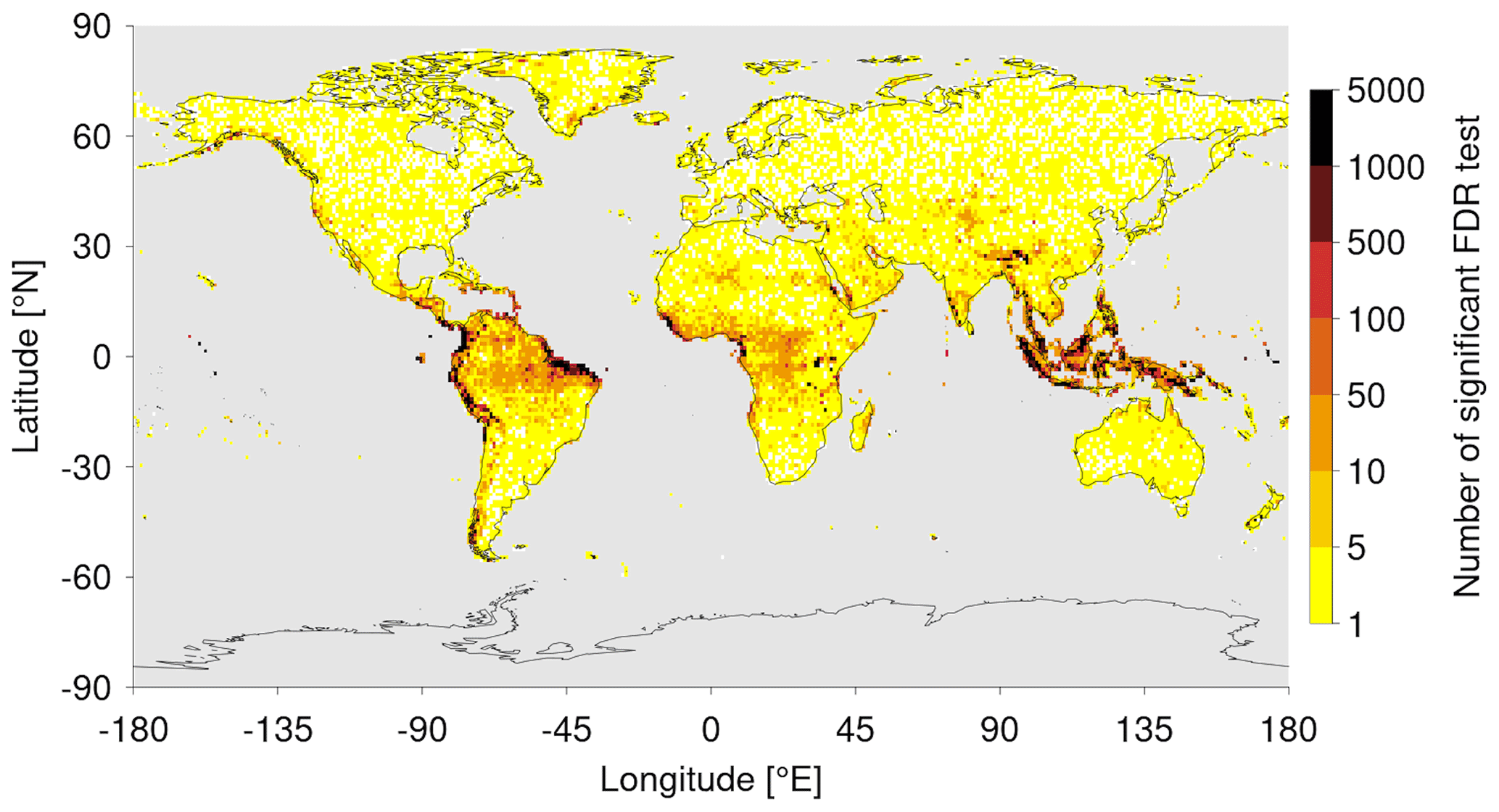
Figure 1 Number of statistical significant correlation coefficients per grid point obtained from the FDR tests of Benjamini and Hochberg (1995), as described in Ventura et al. (2004), applied to multiple (5152) p values associated with the Pearson correlations between yearly maxima time series of individual ensemble members. Note the logarithmic colour scale.

To evaluate the statistical distribution of daily precipitation, Ruff and Pfahl (2023) compared quantiles from the EPS data to three observational data sets and found good agreement in the central European river catchments. For a similar analysis on the global scale with a more pronounced focus on more intense daily precipitation, we select the 99th and 99.99th percentiles at each grid point. Note that all days of a time series, including dry days, are considered for the determination of these percentiles (Pfleiderer et al., 2019). Figure 2 shows the 99th percentile (ca. 0.3-year event) and the 99.99th percentile (ca. 30-year event) from the EPS data (taking all members together) in panels (a–b) and the differences vs. the observational REGEN data in (c–f). High values of the 99th percentile of daily precipitation can generally be found over the tropics and subtropics (see Fig. 2a), especially in the area of the Intertropical Convergence Zone (ITCZ), as well as near complex terrain. Over the extratropical continents, the 99th percentile is slightly lower. The differences vs. the REGEN data set in Fig. 2c and e reveal that EPS data show relatively good agreement over regions where the REGEN observations are trustworthy (black dots). There is generally a slight overestimation of the percentiles in the EPS data, except for some parts of Europe, Mexico and India where REGEN observations indicate higher 99th percentiles. Larger differences can be found over South America, Africa and the Maritime Continent in particular, where the REGEN observations are not considered trustworthy, with values of up to +500 % or −80 %. The absolute and relative differences vs. the CHIRPS and PERSIANN observations in general show similar results (see Fig. S2a, c, e and g). However, there are some large differences also between the observational data sets, e.g. lower 99th percentiles over North America, China and the Maritime Continent in PERSIANN observations; lower 99th percentiles over central Asia in CHIRPS observations; and large differences in the 99th percentile over large parts of Africa between all observational data sets. Similar results are obtained for the 99.99th percentile. Even higher precipitation values from the EPS data are found in the tropics (see Fig. 2b), while there is still relatively good agreement over areas with trustworthy REGEN observations (see Fig. 2d and f). However, the differences vs. the REGEN observations generally increase with higher percentiles. This is also evident for differences in the 99.99th percentile vs. the CHIRPS and PERSIANN observations (see Fig. S2b, d, f and h), while some large differences still remain over the previously mentioned regions between the observational data sets. In summary, the percentiles calculated from EPS data show relatively good agreement with observational estimates over North America and large parts of Europe, central Asia, Australia and South America. With increasing percentiles, the differences vs. observational data sets increase, which might be due to an overestimation of the EPS data or to biases in the representation of very high percentiles in the observations due to a limited length of the time series. Still, bias correction of the EPS data is not considered in this study as the observational data sets show large uncertainties over several parts of the globe. Ruff and Pfahl (2023) also compared the precipitation statistics between each individual ensemble member, but as they found no systematic differences, this analysis is not repeated here.

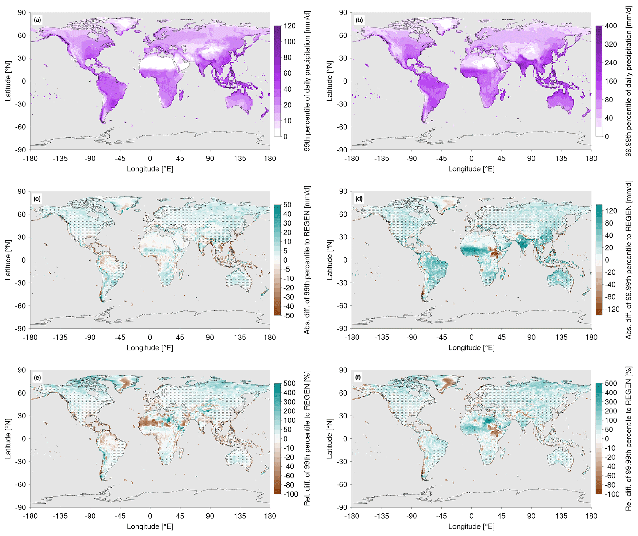
Figure 2 Global distribution of the (a) 99th and (b) 99.99th percentiles of daily precipitation from the EPS data and their (c, d) absolute and (e, f) relative differences vs. the REGEN observations. Stippling in panels (c)–(f) shows where the REGEN observations are trustworthy, as explained in Sect. 2.2.1. Note the non-linear colour scales.

Stationarity of the time series is important for applying the extreme value analysis described in Sect. 3.2. To evaluate the stationarity of the EPS data, Ruff and Pfahl (2023) applied the Mann–Kendall test to several high percentiles and to the yearly number of 100-year precipitation events for the years 2008 to 2019, and they also compared the occurrences of such events to a Poisson distribution of independent events with a constant mean rate. They did not find an indication of temporal non-stationarity in this 12-year period. Here, the same Mann–Kendall test is applied to the yearly maximum of daily precipitation at all global land grid points. In order to evaluate the statistical significance of these multiple tests, again the FDR test is applied (see Fig. S3) as introduced earlier. No significant trend is found for the EPS data. For the observational data sets, also due to the longer time series covering 39 years or more, some areas are associated with significant trends: over a rather evenly distributed area over the globe (for REGEN, 6.7 % of grid points with significant trends), over central Africa and central Asia (for CHIRPS, 0.7 % of grid points with significant trends), or over India and central Asia (for PERSIANN, 1.2 % of grid points with significant trends). Nevertheless, trends are still not significant over most parts of the globe. In order to use a consistent methodology for all data sets and locations, we thus also make the stationarity assumption for the observational time series.

In summary, our analyses show that in most regions, daily precipitation obtained from different members of the ECMWF EPS can be considered statistically independent. Exceptions are some areas over tropical regions of South America and Africa, as well as over the Maritime Continent (see again Fig. 1). Additionally, the model data represent different quantiles of daily precipitation quite well in comparison to three observational data sets (see Figs. 2 and S2), again with the exception of a few regions mostly in the tropics, and have larger differences for very high percentiles. Finally, there is no indication of non-stationarity in the data set over the time frame analysed here. Thus, we consider the EPS data to be suitable for a global analysis of 100-year return values of daily precipitation.

3.2 Determination of return values and confidence intervals

To determine 100-year return values of daily precipitation and their confidence intervals at each grid point, the daily precipitation sums from all ensemble members are used to build long time series. For this investigation, extreme value statistics (see Coles et al., 2001) are applied in order to fit a generalised extreme value distribution (GEV) to a selected sample of block maxima using the maximum likelihood approach. This sample of block maxima is here selected from yearly blocks of daily precipitation. Such an approach leads to 1224 block maxima, to which the GEV can be fitted at each grid point. The best fit of the GEV is accomplished by estimating the location (μ), scale (σ) and shape (ξ) parameters from the maximum likelihood approach. Following Stephenson (2002), the return value v can be computed from these estimated parameters using the following equation:

$$\begin{array}{}\text{(1)}& {\displaystyle }\begin{array}{rl}{\displaystyle }& {\displaystyle }v=\mathit{\mu }+\mathit{\sigma }\cdot {\displaystyle \frac{(x^{\mathit{\xi }}-\mathrm{1})}{\mathit{\xi }}}\\ {\displaystyle }& {\displaystyle }x={\displaystyle \frac{-\mathrm{1}}{\log \left(\mathrm{1}-\frac{\mathrm{1}}{p}\right)}}\end{array}\end{array}$$

in which a certain yearly return period is described by p. The confidence intervals of the return values are computed by the bootstrap resampling method (see Coles et al., 2001). Taking the original set of block maxima, a new set of maxima is drawn with replacement. Then, the previously explained approach of fitting a GEV to a selected sample of block maxima is repeated with the new set of block maxima, and the return value is again determined from Eq. (1). As each procedure leads to a slightly changed return value, the uncertainty can be evaluated by repeating this process several times. Here, it is repeated 1000 times. From the resulting 1000 return values, the 0.025 and 0.975 quantiles are considered to be the confidence intervals of the return value from the original sample of block maxima. This process to determine return values and their confidence intervals from EPS data is also used for all the observational data sets.

At some grid points with very low precipitation amounts during the entire year (e.g. over the Sahara Desert), the best fit of the GEV yields very high estimates of the shape parameter ξ (up to 3). This results in extraordinary high return values compared to neighbouring grid points with low return values. Papalexiou and Koutsoyiannis (2013) analysed estimated shape parameters from GEV fits for over 15 000 globally distributed observational records, using yearly maxima of daily precipitation as block maxima as well. Even for rather short time series of at most 10 years, which are often associated with higher shape parameters than longer time series, the shape parameters all lie between −0.6 and 0.6, independent of their location. However, almost no time series from their observational data set are located in very dry regions such as the Sahara Desert. In order to prevent unrealistic high or low return values but still allow shape parameters outside the range of −0.6 and 0.6 for areas that are typically not covered by observations, grid points with estimated shape parameters above 1 and below −1 and scale parameters above 70 and below −70 are excluded from the analyses in this study.

4 Results

In this section, the estimated 100-year return values of daily precipitation and their confidence intervals are presented. Estimates from the EPS data are compared to the observational estimates based on REGEN, CHIRPS and PERSIANN.

4.1 Return values

Global estimates of 100-year return values of daily precipitation from the EPS data set are shown in Fig. 3a. Generally, higher return values can be found in the tropics and parts of the subtropics, with values between 400 and 600 mm d⁻¹ over most parts of India and near the Himalaya, as well as values around 300 mm d⁻¹ for tropical regions, while return values decrease towards the poles. A 100-year event in the midlatitudes is typically associated with values of 50–100 mm d⁻¹, while usually dry regions such as the Sahara Desert and the Taklamakan Desert are associated with very low return values of around 30 mm d⁻¹. Still, such extreme events over these very dry regions typically lead to an exceptional exceedance of the annual precipitation amount: with values of about 300 %–700 % for the two latter regions (see Fig. S4).

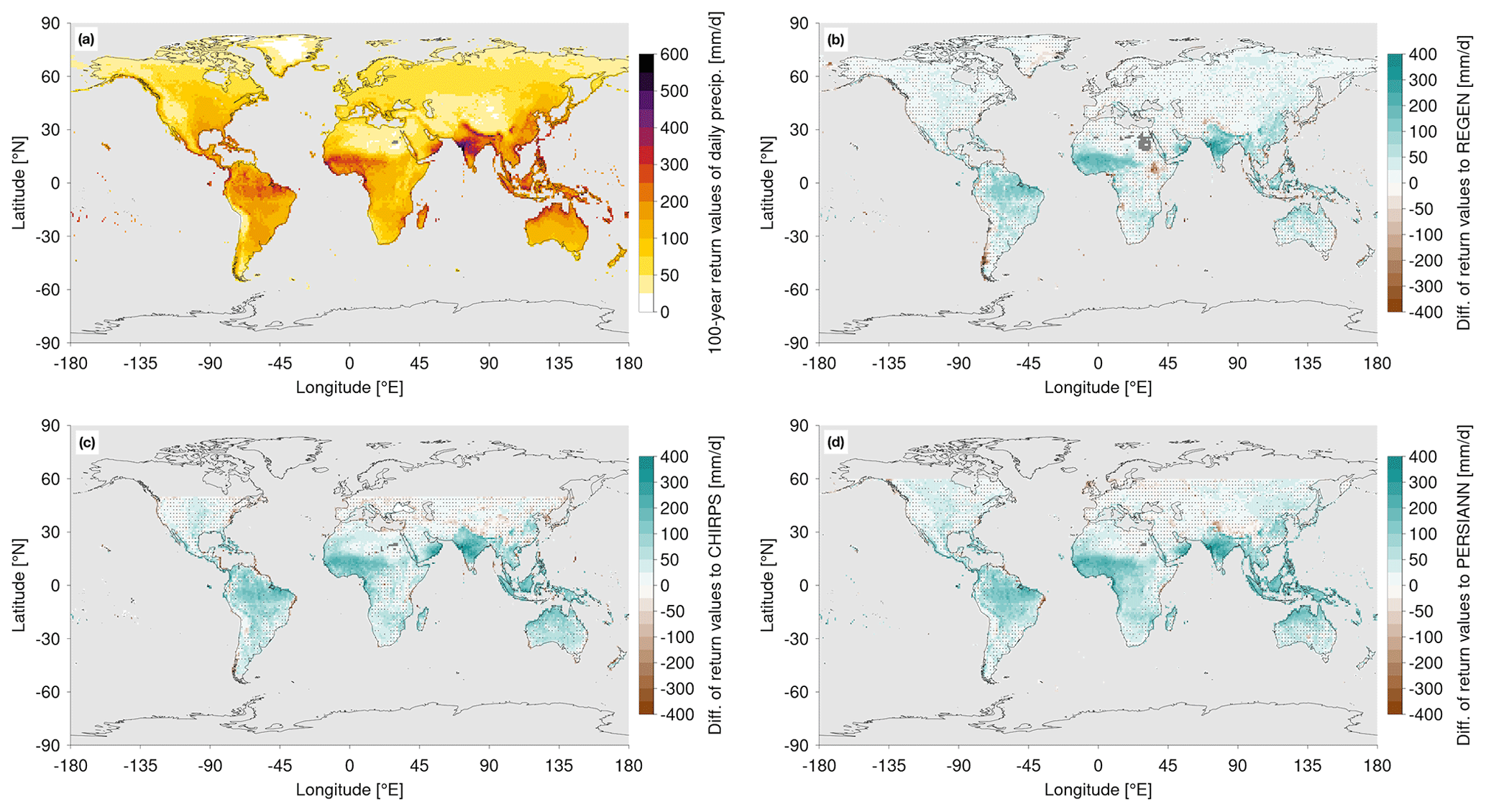
Figure 3 (a) Global distribution of 100-year return values of daily precipitation estimated from EPS data and their differences vs. the observational estimates from (b) REGEN, (c) CHIRPS and (d) PERSIANN. Dark grey shading indicates grid points for which the GEV parameters are outside the allowed range, and thus no return values can be estimated. Stippling in panels (b)–(d) shows where the confidence interval of the EPS data overlaps with the confidence interval from the specific observational data set. Note the non-linear colour scales.

A comparison with the observational data set REGEN shows generally higher EPS estimates over large parts of the globe and very large differences in several tropical and subtropical regions (Fig. 3b). The 100-year return values from the EPS data are clearly higher, e.g. over India (by 200–400 mm d⁻¹), western Africa (by 100–300 mm d⁻¹) and over the Amazon (by 50–150 mm d⁻¹), with large differences also existing for much-lower return periods at individual locations (see Fig. S5c and d). Additionally, the confidence intervals of the EPS data do not overlap with the REGEN data in these regions (even for much lower return periods; see Fig. S5c and d); the differences are thus statistically significant. Over other parts of South America, the southern half of Africa and Australia, the EPS estimates are about 50 mm d⁻¹ higher, but the confidence intervals overlap in parts of these areas. The midlatitudes do not show large differences in the estimated return values (similar for lower return periods at individual locations; see Fig. S5a and b). However, over parts of Chile, the Abyssinian Plateau in East Africa and over some coastal areas in Southeast Asia, the EPS data are associated with lower return values than the REGEN data (mostly no overlap of confidence intervals). Overall, the confidence intervals of EPS and REGEN return value estimates overlap at 55.6 % of the grid boxes. The differences in EPS return values vs. the CHIRPS and PERSIANN observational estimates (Fig. 3c and d) are very similar to each other. The confidence intervals of EPS and CHIRPS overlap at 48.6 % of the grid boxes, and for EPS and PERSIANN this overlap is 51.6 %. Furthermore, the CHIRPS and PERSIANN results are mostly consistent with the differences vs. the REGEN estimates described above. However, the strongly negative differences over Chile and the Abyssinian Plateau do not occur for the CHIRPS and PERSIANN data. Additionally, the positive differences over India, Southeast Asia and Australia are even slightly larger. It should be kept in mind here that over the tropical parts of South America and the Maritime Continent in particular, the EPS estimates are less trustworthy than in other regions due to methodological issues associated with interdependence between the ensemble members (see again Sect. 3.1).

4.2 Confidence intervals

Confidence intervals (CIs) on a 95 % level are determined for each return value estimate. To compare the confidence interval ranges (that is, the difference between upper and lower bounds) between data sets, on the one hand, in Fig. 4a and b they are shown relative to the corresponding return value estimates, as higher return values are typically associated with larger confidence intervals. In this way, the relative uncertainty in the 100-year return values is quantified. On the other hand, Fig. 4c and d shows the absolute confidence interval ranges, quantifying the absolute uncertainties.

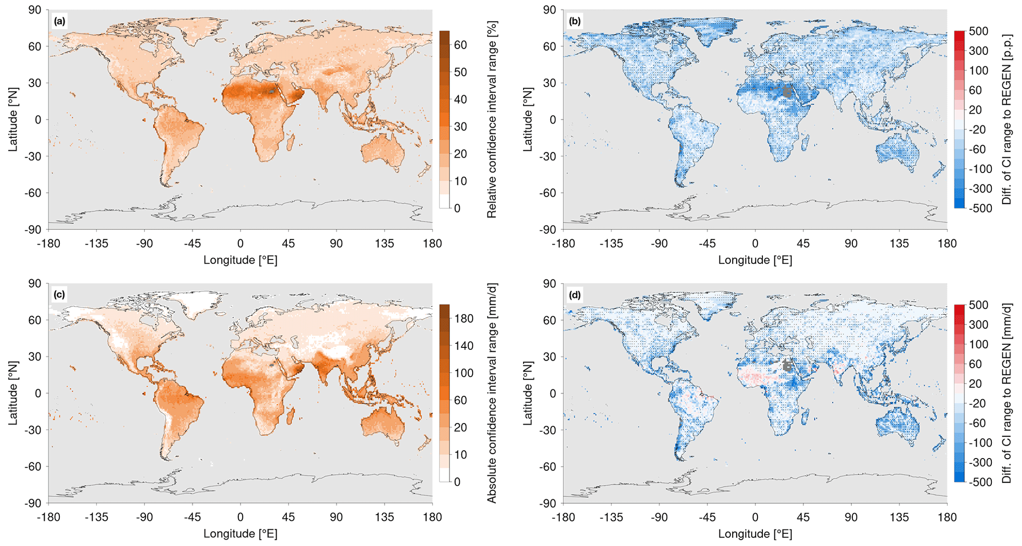
Figure 4 (a, c) Global distribution of EPS data confidence interval ranges on a 95 % level and (b, d) their differences vs. the observational estimates from REGEN for (a, b) the relative range, relative to the associated return values, and (c, d) the absolute range of these confidence intervals. Dark grey shading indicates grid points for which the GEV parameters are outside the allowed range, and thus no return values can be estimated. Stippling in panels (b) and (d) shows where the confidence interval of the EPS data overlaps with the confidence interval from the REGEN observations. Note the non-linear colour scales.

The largest relative uncertainties are found in tropical and subtropical regions. Over the Sahara Desert and the southeastern part of the Arabian Peninsula in particular, the relative CIs range from 30 % to 65 %, while poleward of 30° N and 30° S, the range of the relative CIs lies between 10 % and 20 % (see Fig. 4a). This pattern of relative CIs strongly correlates with the ratio of a 100-year event vs. the annual precipitation amount in Fig. S4. Over regions where a 100-year event represents a multiple of the annual precipitation amount, the daily precipitation distribution is typically associated with a rather short and thick tail. An estimation of very high percentiles from such a distribution is more difficult and leads to higher uncertainties. As mentioned before, higher return values are associated with higher CIs, as shown by the absolute values in Fig. 4c. The tropics and several subtropical areas have the highest absolute CI ranges with typical values of 50–150 mm d⁻¹. Absolute CIs over the midlatitudes typically lie around 10 mm d⁻¹.

The differences in the relative CI ranges between the EPS and REGEN data sets are shown in Fig. 4b. Over almost all continental areas, the relative uncertainties are reduced in the EPS data compared to REGEN, with typical differences on the order of 50–100 percentage points (p.p.). Over specific regions such as the west coast of South America, the Sahara Desert and the Arabian Peninsula, this decrease is even larger (−200 p.p. to −800 p.p.), while the CIs mainly overlap with each other in these regions. A slight increase in the relative uncertainty by around 10 p.p. is found for some grid points over the Amazon, West Africa, India and China. In terms of absolute CI ranges (Fig. 4d), the uncertainty is often reduced in the EPS data compared to REGEN by up to 300 mm d⁻¹ over the tropics and subtropics and by around 20 mm d⁻¹ over the midlatitudes. Note that this corresponds to a reduction by at least a factor of 2 – substantially reduced uncertainty in most regions. There are a few more extended (compared to the relative CI ranges) areas of larger absolute uncertainties in the EPS data over the Amazon, West Africa and India, with increases of 20–100 mm d⁻¹. These are also regions where the CIs do not overlap.

Similar results are found for both relative and absolute uncertainties, taking the CHIRPS data for comparison. The relative CI range is smaller in the EPS data over almost all regions (see Fig. S6a), and the magnitude of this reduction is typically even larger (around −100 p.p.) than for REGEN, except for the Sahara Desert. Differences in the absolute uncertainty compared to CHIRPS are again similar for REGEN but with a more enhanced and broader increase of up to 300 mm d⁻¹ in the southeast of the Arabian Peninsula (see Fig. S6c). Finally, the uncertainty in EPS is also reduced compared to PERSIANN, with similar patterns over the continents for REGEN and CHIRPS (see Fig. S6b and d). Note that a co-occurring increase in absolute uncertainty and decrease in relative uncertainty in return value estimates are linked to substantially higher return value estimates in the EPS data.

The main advantage of the model-generated EPS data compared to the observational data sets is the extraordinary length of the time series that is used for the 100-year return value estimate. However, it is not directly evident how large this effect of the length of the time series is on the return value estimate and its uncertainty. In order to quantify this effect, the determination of the 100-year return value and its confidence intervals is repeated for different sample sizes of the yearly EPS block maxima, starting with a sample size of 60 as this is roughly the length of the observational data sets. The results show that the estimated return values do not depend strongly on the sample size and increase only slightly with increasing sample sizes over all parts of the globe (not shown). Figure 5 shows the distribution of 1000 return value estimates and its confidence intervals for sample sizes of 60, 120, 240, 480 and 1200 for one grid point over Berlin, Germany (52° N, 13° E). As mentioned previously, the increase in the return value estimate with higher sample sizes is rather small. This indicates that the systematic overestimation of the EPS return values in many parts of the world is likely due to biases of the model or the observational data sets and is not caused by the systematic differences in sample size. However, there is a clear reduction in the uncertainty in the 100-year return value with a larger sample size. Thus, the sampling effect can clearly explain the reduced uncertainty in the EPS data set.

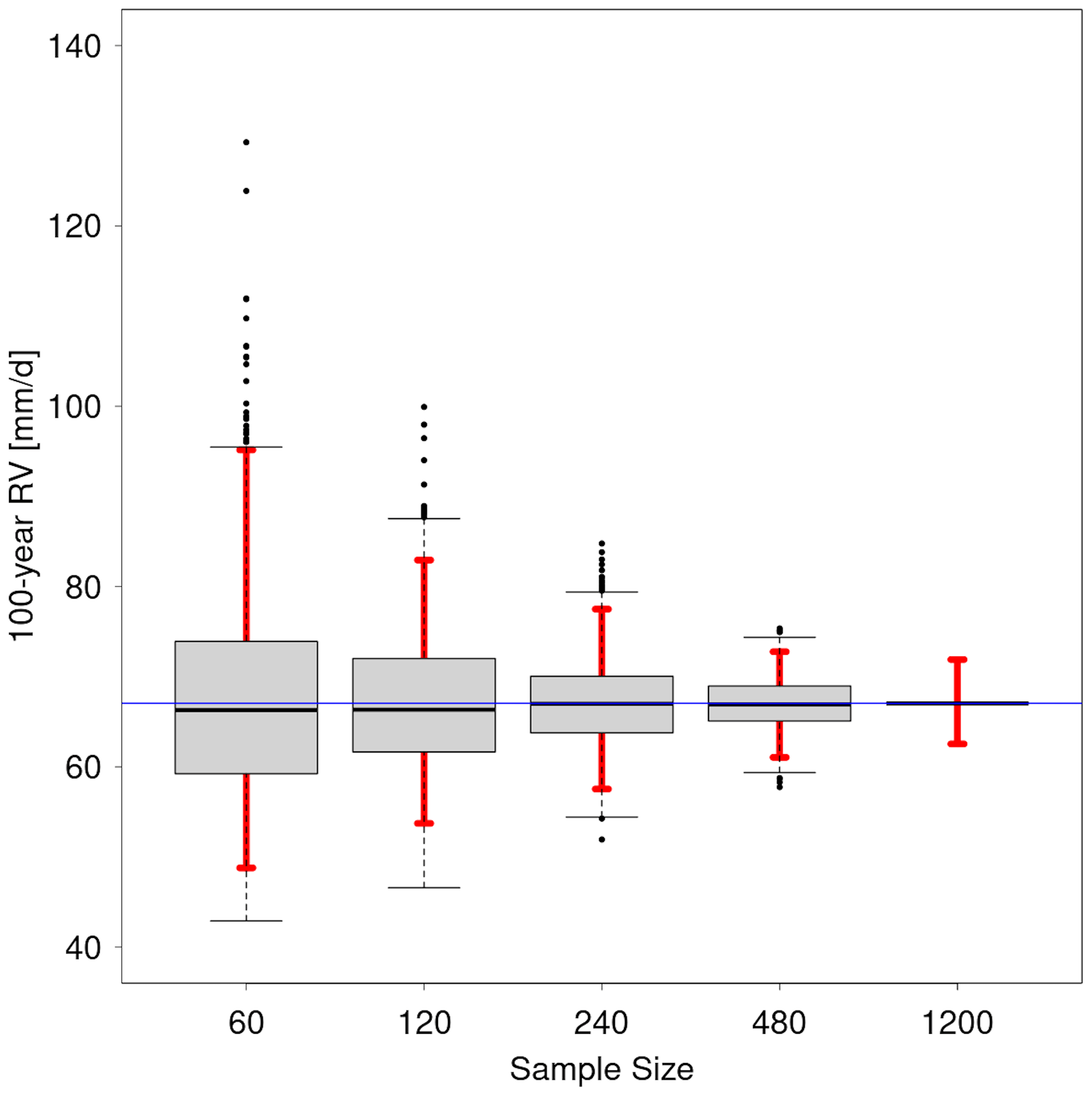
Figure 5 Boxplot distribution of 1000 return value estimates of a 100-year event obtained from subsampling the EPS block maxima with different sample sizes for a single grid point over Berlin, Germany (52° N, 13° E). The boxplot whiskers represent the data point, which is no more than 1.5 times the interquartile range from the box. The red bars indicate the 95 % confidence interval. The blue line indicates the 100-year estimate from the largest sample size of 1200.

5 Discussion and conclusion

The aims of this study have been to determine 100-year return values of daily precipitation and their confidence intervals (CIs) on a global scale from a large data set of model-generated events and to evaluate the differences vs. three observational data sets (REGEN, CHIRPS and PERSIANN). Quantification of such extreme return values is crucial for properly setting up flood protection measures and also because such extreme events are expected to occur more frequently in a warmer climate. The large set of simulated global daily precipitation fields has been obtained from operational ensemble weather prediction data by the ECMWF, following the approach of Breivik et al. (2013) and Ruff and Pfahl (2023). Our statistical analyses show that when using the 10th forecast days from these simulations, annual precipitation maxima are independent between the different ensemble members in most regions except for some tropical areas over South America, Africa and the Maritime Continent. There, extreme precipitation events are correlated between different ensemble members such that these events can not be considered independent. This reduces the effective sample size of events for the analyses and decreases the length of the precipitation time series, leading to less-trustworthy results of 100-year return values. Biases in the climatological distribution of extreme precipitation with respect to the observational data sets, evaluated through the 99th and 99.99th percentile, are relatively small in most regions of North and South America, Europe, central Asia, and Australia but larger for other regions and generally increase for very high percentiles. Additionally, there is no significant trend in the occurrence of intense precipitation over the 12 years at all grid points, and the EPS data can thus be considered stationary in time. With the help of extreme value statistics, 100-year return values and the associated confidence intervals on a 95 % level are determined and compared to estimates from the observational data sets.

Based on these EPS data, the largest 100-year return values of daily precipitation, which are computed over 1°×1° grid boxes, occur in the tropics and subtropics, with a maximum of up to 600 mm d⁻¹ (absolute CI range of 150 mm d⁻¹) over India and typical values around 300 mm d⁻¹ (absolute CI range around 100 mm d⁻¹) for most of the other tropical and subtropical regions. The return values decrease towards the poles, with values of 50–100 mm d⁻¹ (absolute CI range of 10 mm d⁻¹) over the midlatitudes. Such an extreme event would typically amount to about 10 %–20 % of annual mean precipitation (20 %–50 % for Australia), but in dry regions such as the Sahara Desert, the estimated 100-year return value even exceeds the annual mean precipitation by a factor of up to 7. The 100-year return values from the EPS data are in general agreement with other studies of multi-year precipitation extremes. For instance, Rodrigues et al. (2020) determined 10-year return values for Brazil and found slightly lower values and a local maximum of 200 mm d⁻¹ further towards the east coast. Gründemann et al. (2023) studied 100-year return values over global land areas based on several statistical approaches and a data set obtained from a combination of satellite observations, reanalyses and gauge data. They found similar spatial patterns as were documented here but lower return values over, for instance, the Sahel, the east coast of the Arabian Peninsula and parts of India. Also, the comparison with the observational data sets in this study indicates systematically higher return values in the EPS data set over most of the globe. In many regions, in particular in the extratropics, the confidence intervals of EPS and observational estimates still overlap. Larger, also statistically significant differences are obtained in some tropical regions where the EPS method is less robust due to interdependence of ensemble members and/or general biases in the precipitation climatology, but they also occur over other areas where the data set performs well in our statistical evaluation, such as parts of northeastern South America, western tropical Africa, India and eastern China. This might be due to model deficiencies, e.g. in the representation of convective extreme precipitation in the tropics. However, it may also point to a systematic underestimation of extreme daily precipitation events in observations. Such a potential underestimation might have important consequences for practical applications and should be considered in estimates of probable maximum precipitation for designing flood protection measures.

The relative uncertainty in the 100-year return values is quantified through relative confidence interval ranges, which typically lie within 10 %–30 % for most of the regions but can be higher than 50 % over the Sahara Desert and the Arabian Peninsula. An important result is that these relative uncertainties (and in most regions also the absolute CI ranges) are substantially reduced in the EPS data compared to observational estimates. This reduction is typically on the order of 50–100 p.p. but can locally amount to up to 500 p.p., e.g. over the Sahara Desert and the Arabian Peninsula.

Observation-based estimates of very high percentiles of daily precipitation contain uncertainties due to the finite length of observational time series; the ambiguous choice of the statistical method to estimate extreme values and spatial inhomogeneities from, e.g. an uneven distribution of rain gauges; and trends from anthropogenic climate change. The two latter limitations are reduced using a weather prediction model for a rather short period of time (12 years). Additionally, the systematic and substantial reduction in statistical uncertainty in this study is due to the much longer time series and is the main advantage of the model-generated EPS data compared to the observational data sets. However, we do not claim that these model data are superior to observations in any other way but rather show the advantages and disadvantages of both model-generated EPS and observational data when estimating 100-year daily precipitation events on a global scale and their uncertainties.

Our approach to estimate 100-year precipitation return values from EPS data has several limitations, as also discussed by Ruff and Pfahl (2023). First, the model-generated precipitation data are affected by model biases and the imperfect representation of specific processes in the model, especially over the tropics. Such biases are assumed to be particularly large for small-scale convective precipitation events, which is one reason why we focus on larger-scale events on a 1°×1° grid. Second, the time span of the forecast data is limited to 12 years (2008–2019), which comes along with a limited sampling of large-scale boundary conditions. Therefore, the entire range of (multi-)decadal variability in the climate system is not reproduced in the data set. Third, there is a certain influence of anthropogenic forcing in the data set in specific regions, as mentioned in Sect. 3.1, which can lead to temporal inhomogeneities. However, our trend analyses show that this is mainly restricted to a few areas. Fourth, the method does not work well in regions where the ensemble members are not independent from each other, which mainly includes the tropical regions of South America and Africa as well as the Maritime Continent.

In future research, the approach used here may be applied to events with different return periods and also to other weather prediction ensemble data sets, which may help in clarifying the reasons for the systematically higher return values in the EPS data compared to observations. Finally, large initial condition ensemble simulations with climate models may be used to investigate the influence of climate warming on 100-year precipitation events.