Heat wave characteristics: evaluation of regional climate model performances for Germany

Heat waves are among the most severe climate extreme events. In this study, we address the impact of increased model resolution and tailored model settings on the reproduction of these events by evaluating different regional climate model outputs for Germany and its near surroundings between 1980–2009. Outputs of an ensemble of six EURO-CORDEX models with 12.5 km grid resolution and outputs from a high-resolution (5 km) WRF (Weather Research and Forecasting) model run are employed. The latter was especially tailored for the study region regarding the physics configuration. We analyze the reproduction of the maximum temperature, number of heat wave days, heat wave characteristics (frequency, duration and intensity), the 2003 major event, and trends in the annual number of heat waves. E-OBS is used as the reference, and we utilize the Taylor diagram, the Mann–Kendall trend test and the spatial efficiency metric, while the cumulative heat index is used as a measure of intensity. Averaged over the domain, heat waves occurred about 31 times in the study period, with an average duration of 4 d and an average heat excess of 10 ^∘C. The maximum temperature was only reproduced satisfactorily by some models. Despite using the same forcing, the models exhibited a large spread in heat wave reproduction. The domain mean conditions for heat wave frequency and duration were captured reasonably well, but the intensity was reproduced weakly. The spread was particularly pronounced for the 2003 event, indicating how difficult it was for the models to reproduce single major events. All models underestimated the spatial extent of the observed increasing trends. WRF generally did not perform significantly better than the other models. We conclude that increasing the model resolution does not add significant value to heat wave simulation if the base resolution is already relatively high. Tailored model settings seem to play a minor role. The sometimes pronounced differences in performance, however, highlight that the choice of model can be crucial.

1 Introduction

Heat waves are climatological extreme events with severe negative impacts on organisms and ecosystems. Their effects can be illness, large-scale mortality, substantial losses in agricultural production, forest fires and an increased energy demand for cooling (Beniston et al., 2007; Ciais et al., 2005; Robine et al., 2008; Kyselý et al., 2011; Bastos et al., 2014; Urban et al., 2017). Especially in the midlatitude zones, heat waves are regarded as a major cause of weather-related human mortalities (Luber and McGeehin, 2008; Plavcová and Kyselý, 2019). In Europe, they are a regular part of the summer climate (Vautard et al., 2013), and an increasing trend in the number of summer heat waves across recent decades was reported, along with a tendency for them to prolong (Della-Marta et al., 2007; Kyselý, 2010; Valeriánová et al., 2017; Saeed et al., 2017). According to Fischer and Schär (2010), the frequency and length of heat waves have nearly tripled and doubled, respectively, over the period 1880–2005 in western European regions. Especially since the turn of the millennium, Europe has experienced multiple extraordinary heat waves (Lhotka et al., 2018b). Two of the most prominent events were the heat episodes in 2003 over western Europe (Fink et al., 2004) and the 2010 event over eastern Europe and Russia (Schneidereit et al., 2012). In the more recent past, severe summer heat episodes took place in central Europe in 2013 (Lhotka and Kyselý, 2015a), 2015 (Hoy et al., 2017) and, especially, in 2018 (e.g., Vogel et al., 2019; Rousi et al., 2023). In the context of climate change, heat waves are expected to become more frequent, more intense and longer lasting in the future around the globe (Meehl and Tebaldi 2004; Lau and Nath 2014; Lemonsu et al. 2014; Seneviratne et al., 2014; Diffenbaugh and Ashfaq 2010). Coumou and Rahmstorf (2012) estimate that the probability of severe events like that in 2003 over western Europe has increased by a factor of 2–4 because of global warming. Shifts of the temperature distribution are considered the primary drivers of these changes (Ballester et al., 2010; Lau and Nath, 2014). According to Fischer and Schär (2010), a larger variance of the summer temperature distribution in future climates is another possible driver. Lhotka et al. (2018a) additionally emphasize the increased temporal autocorrelation of the daily maximum temperature, which leads to more persistent heat waves, as a potential driver.

Regional climate models (RCMs) are used to analyze and understand such changes at the regional scale and to allow projections of the characteristics of future heat wave events. For better interpretation of future climate scenarios and their uncertainties and limitations, it is important to evaluate RCM simulations of the recent or historical climate to detect biases, which are usually present despite the added value compared to GCMs (Lhotka et al., 2018a; Plavcová and Kyselý, 2019; Lin et al., 2022). The availability and reliability of RCM simulations have rapidly evolved in recent years (Štepánek et al., 2016). This is also due to concerted downscaling projects and initiatives such as PRUDENCE (Christensen and Christensen, 2007), ENSEMBLES (van der Linden and Mitchell, 2009) and, most recently, CORDEX (Giorgi et al., 2009). In the recent past, there have been several heat-wave-related studies using data from the CORDEX initiative for different parts of the world that have focused on both past periods and future scenarios. For the EURO-CORDEX domain, the focus was on the evaluation of the RCM's capability in simulating past heat episodes in France (Ouzeau et al., 2016) and all of Europe (Vautard et al., 2013; Lhotka et al., 2018a; Plavcová and Kyselý, 2019; Lin et al., 2022) as well as on the development of future episodes under different scenarios for Portugal (Cardoso et al., 2019), France (Ouzeau et al., 2016), the Mediterranean area (Molina et al., 2020) and all of Europe (Lhotka et al., 2018b; Smid et al., 2019; Machard et al., 2020; Lin et al., 2022). Regarding the rest of the globe and the other CORDEX domains, evaluation studies have been carried out for Africa (Russo et al., 2016), East Asia (Wang et al., 2019b) and South America (Silva et al., 2022). Furthermore, projection studies were performed for Africa (Dosio, 2017), Afghanistan (Aich et al., 2017), South America (Feron et al., 2019), China (Wang et al., 2019a), the MENA region (Varela et al., 2020), the eastern Mediterranean (Wedler et al., 2023), East Asia (Kim et al., 2023) and the entire globe (Coppola et al., 2021). In the mentioned studies, different horizontal grid resolutions of the models were used and the effects of increased resolution were often analyzed, which led to different findings: Zeng et al. (2016) and Vichot-Llano et al. (2021), for example, found that higher resolution leads to better reproduction of temperature fields, while Di Luca et al. (2013) came to the conclusion that the potential of increased resolution to add value is small. It is important to consider the differences between the compared resolutions in such studies (Petrovic et al., 2022). Besides the model resolution, the model setup (the domain configuration and physical parameterizations for the selected target region) is a crucial factor for reliable simulations (e.g., Stoelinga et al., 2003; Kumar et al., 2010). For the temperature simulation, Vautard et al. (2013) found that it is primarily sensitive to convection and microphysics schemes. They emphasize that a large part of the model spread in their study can be attributed to different parameterizations. Moreover, they draw a connection between parameterizations and different spatial resolutions. Mooney et al. (2013) found that the simulated temperature showed relatively high sensitivity to the land surface model, some sensitivity to the radiation schemes, and minor sensitivity to the microphysics and planetary boundary layer (PBL) schemes. They concluded that the optimal parameterization combination had a strong dependence on the region and season. Kotlarski et al. (2014) state that bias spreads between different configurations of the same model can be similar to those between different models.

To our knowledge, there is no study that presents an evaluation of the EURO-CORDEX RCM's capability to reproduce heat wave characteristics for Germany, which motivated us to perform the present analysis. At the same time, this study is the follow-up to the model comparison study for droughts performed by Petrovic et al. (2022). The thematic proximity is obvious, since heat and drought are often, but not always, related to each other. We analyze a variety of RCM simulations, i.e., a 5 km, three-domain Weather Research and Forecasting (WRF, Skamarock et al., 2008) model run and an ensemble of six EURO-CORDEX realizations at 12.5 km horizontal resolution. The setup for the WRF model was precisely determined for Germany. Intuitively, one would expect the WRF model to give better performance when simulating hot temperatures due to its higher resolution and focus on the target region compared to the EURO-CORDEX runs. The WRF model was shown to be capable of simulating spatiotemporal features of heat wave events over a large domain (Wang et al., 2019b). To attribute potential WRF performance benefits to a resolution or a settings effect, we additionally include a 15 km WRF simulation configuration in our analysis which is slightly coarser than that for the EURO-CORDEX standard. Therefore, following on from the drought study (Petrovic et al., 2022), the objectives of this study are as follows:

1. Evaluate the performance of regional climate models in reproducing hot temperatures and associated heat wave characteristics by employing a six-member EURO-CORDEX ensemble and a high-resolution WRF run. The EURO-CORDEX RCMs and WRF differ in resolution, while the model physics configuration is different for every single RCM.

2. Obtain insights about the heat wave history of Germany and its near surroundings between 1980 and 2009.

For this purpose, the results are evaluated and compared to observations. Specifically, we analyze the reproduction of the daily maximum temperature, the number of heat wave days, heat wave characteristics (frequency, duration and intensity), trends in the number of heat waves per year, and the heat wave event in 2003.

Moreover, we compare the new core findings for heat waves with those from the aforementioned drought analysis (Petrovic et al., 2022) in terms of similarities and differences.

2 Data

In this study, data from the same sources as in Petrovic et al. (2022) are used. While monthly data on precipitation and minimum and maximum temperatures were used in that study, the daily values of the maximum (surface) temperature (T_max) are employed here.

We use data from an ensemble of six EURO-CORDEX RCM simulations. Each of the experiments were conducted with 0.11^∘ (≈ 12.5 km) horizontal grid resolution and cover the EUR-11 CORDEX domain. Outputs from the following RCMs were used: COSMO-CLM, ALADIN 6.3 (hereafter referred to as ALADIN in the text), REMO2015 (REMO), RegCM 4.6 (RegCM), RACMO 2.2e (RACMO) and RCA4. The boundary conditions for all the runs were obtained from the global ERA-Interim reanalysis (Dee et al., 2011). When this analysis was initiated, these runs were the only ones that covered the study period 1980–2009 and contained the relevant meteorological variables.

In addition to the EURO-CORDEX data, we included the outputs from the ERA-Interim-forced reanalysis WRF run for the time period 1980–2009 from Warscher et al. (2019). These simulations were preceded by a comprehensive search and final identification of the optimal model physics and parameterization configuration for the target region, i.e., Germany (Wagner and Kunstmann, 2016). This is the first major difference from the EURO-CORDEX outputs, which were aimed at the entire EUR-11 CORDEX domain (Giorgi et al., 2009). A two-domain setup with one-way nesting was employed to downscale the ERA-Interim reanalysis of approx. 75 km. The horizontal grid resolution of the innermost domain, which frames Germany and its near surroundings, is 5 km. This increased resolution is the second major difference from the EURO-CORDEX outputs. As mentioned above, we also used the outputs from the 15 km second WRF domain in the same run. Therefore, we will refer to WRF@5 km and WRF@15 km from hereon to distinguish between the two runs.

More detailed information about the EURO-CORDEX RCMs and an overview of the different model physics configurations for all runs can be obtained from Tables 1 and 2 in Petrovic et al. (2022). The gridded observational data set from E-OBS (Haylock et al., 2008), version 23.1e, with 0.1^∘ (≈ 11.1 km) horizontal grid resolution serves as a reference.

The study region extends from 47 to 55^∘ N and from 6 to 15^∘ E so that it contains Germany and its near surroundings. The WRF and E-OBS data were regridded using bilinear interpolation to match the horizontal grid resolution of the EURO-CORDEX RCMs.

3 Methods

3.1 Analysis of daily maximum temperature reproduction

Since T_max is the main variable determining heat waves, the grid-cell-based summer values (June, July, August) are first analyzed. We use the Taylor diagram (Taylor, 2001), which provides a succinct visual statistical summary of the agreement between patterns, including their correlation, their root-mean-square difference, and the ratio of their variances or standard deviations (Taylor, 2001). Moreover, we calculate the density plot to visualize and compare the distributions of the values of the individual data sets. From spatially and temporally averaged daily values, we calculate the mean bias values in order to be able to draw conclusions about the role of the model bias for further results. It must be noted that both a good simulation of the right tail of the temperature frequency distribution and the persistence of the high temperatures is important for the reproduction of heat waves (Lhotka et al., 2018a).

3.2 Heat wave definition

There is no universal definition of a heat wave. In fact, there are multiple definitions that include different metrics and criteria depending on the region, season and purpose of the study (Feron et al., 2019; Becker et al., 2022). Generally, it describes a period of consecutive days with conditions excessively higher than normal (Perkins et al., 2012). Here, we define a heat wave as an event lasting at least 3 consecutive days where the 90th percentile of T_max is exceeded on each calendar day of the study period (Fischer and Schär, 2010). Therefore, the 90th percentile for each calendar day and each grid cell from each data set was calculated first. This was done individually for each data set to circumvent the T_max biases among the different models (Vautard et al., 2013; Lhotka et al., 2018b). We only address summer heat waves in this study.

3.3 Analysis of heat wave characteristics

Based on the heat wave definition described above, we calculate the number of heat wave days and number of heat waves for each grid cell for the whole study period 1980–2009. Based on the number of heat wave days and heat waves, we determine the mean duration of heat waves for each grid cell from each data set. In order to describe the mean heat wave intensity, we use the cumulative heat index as a measure (e.g., Katavoutas and Founda, 2019; Perkins-Kirkpatrick and Lewis, 2020). This refers to the integration of heat exceedance above the 90th percentile threshold for all heat wave days during a heat episode or whole season:

$$\begin{array}{}\text{(1)}& \mathrm{CumHeat}=\sum _{i=\mathrm{1}}^n\mathrm{\Delta }(T_{\text{max},i}-T_{\text{max},\text{P90},i}),\end{array}$$

where i indicates the calendar day of the heat wave event and $T_{\text{max},\text{P90},i}$ is the 90th percentile of T_max for day i and each grid cell. To get the mean intensity of heat waves, we integrated all excess values for the whole study period and divided the results by the number of heat waves for each grid cell of each data set. For each aspect (number of heat wave days, number of heat waves, mean heat wave duration and mean heat wave intensity), we calculate the domain mean value for every data set. In the next step, we subtract the E-OBS reference domain from each RCM domain to get the bias patterns and also calculate the domain mean values. To further evaluate the spatial agreement between the reference and each RCM, we utilize the spatial efficiency (SPAEF) metric (Demirel et al., 2018; Koch et al., 2018). The SPAEF is a multiple-component performance metric for the comparison of spatial patterns. It is calculated as

$$\begin{array}{}\text{(2)}& \mathrm{SPAEF}=\mathrm{1}-\sqrt{(\mathit{\alpha }-\mathrm{1}{)}^{\mathrm{2}}+(\mathit{\beta }-\mathrm{1}{)}^{\mathrm{2}}+(\mathit{\gamma }-\mathrm{1}{)}^{\mathrm{2}}},\end{array}$$

where α is the Pearson correlation coefficient between the observed (obs) and simulated (sim) patterns,

$$\begin{array}{}\text{(3)}& \mathit{\beta }=\left({\displaystyle \frac{{\mathit{\sigma }}_{\text{sim}}}{{\mathit{\mu }}_{\text{sim}}}}\right)/\left({\displaystyle \frac{{\mathit{\sigma }}_{\text{obs}}}{{\mathit{\mu }}_{\text{obs}}}}\right),\end{array}$$

as the fraction of the coefficient of variation that represents the spatial variability, and

$$\begin{array}{}\text{(4)}& \mathit{\gamma }={\displaystyle \frac{{\sum }_{i=\mathrm{1}}^n\text{min}(K_i,L_i)}{{\sum }_{i=\mathrm{1}}^n{K}_i}},\end{array}$$

as the overlap between the histograms of the observed (K) and simulated (L) patterns, both of which contain the same number n of bins. To calculate γ, we use the z score of the patterns, which allows the comparison of two variables with different units. The number of values in each bin i in the histograms of K and L is counted. Afterwards, for each bin, the lower of the two values is taken to ensure that the number of common values is used. Thereafter, these numbers are summed and divided by the total number n of values in K or L. The SPAEF has a predefined range between −∞ and 1, where 1 corresponds to ideal agreement between two patterns. The three components are independent of each other and typically equally weighted so that they complement each other in a meaningful way and provide holistic pattern information. In this way, instead of exact values on the grid scale, global features such as distribution and variability are evaluated (Koch et al., 2018).

3.4 Heat wave trend analysis

In order to investigate the temporal characteristics of heat wave occurrences, we apply the non-parametric Mann–Kendall trend test approach (Mann, 1945; Kendall, 1975). For this purpose, we first count the number of heat waves per year for each grid cell to obtain the annual development. Then the test is applied to the resulting time series for each grid cell to detect significant monotonic trends at a significance level of 0.05. The Mann–Kendall test is based on the correlation between the ranks of a time series and their time order.

For a time series x₁x₂x₃…x_n, the Mann–Kendall test statistic S is given by

$$\begin{array}{}\text{(5)}& S=\sum _{i=\mathrm{1}}^{n-\mathrm{1}}\sum _{j=i+\mathrm{1}}^n\text{sign}(x_j-x_i),\end{array}$$

with

$$\begin{array}{}\text{(6)}& {\displaystyle }\text{sign}(x_j-x_i)=\text{sign}(R_j-R_i)=\mathrm{1}\text{ if }{x}_j-x_i>\mathrm{0}\text{(7)}& {\displaystyle }\text{sign}(x_j-x_i)=\text{sign}(R_j-R_i)=\mathrm{0}\text{ if }{x}_j-x_i=\mathrm{0}\text{(8)}& {\displaystyle }\text{sign}(x_j-x_i)=\text{sign}(R_j-R_i)=-\mathrm{1}\text{ if }{x}_j-x_i<\mathrm{0},\end{array}$$

where “sign” represents an indicator function, n is the number of data points, and R_i and R_j are their respective ranks. A positive S statistic indicates an increasing trend; a negative one indicates a decreasing trend.

3.5 The 2003 heat wave event

The heat wave and drought event in the summer months of 2003 in central Europe is considered to be one of the most severe extreme events to have occurred in the last few decades. It caused 70 000 excess deaths (Poumadere et al. 2005; Robine et al., 2008), a distinct decrease in plant productivity, crop failures (Bastos et al., 2014) and a record breaking loss of Alpine glacier mass (Braithwaite et al., 2013). This is why the event is also considered a “mega heat wave” (Barriopedro et al. 2011; Vautard et al., 2013).

We investigate the capability of the RCMs to reproduce a single extreme event of this kind in terms of intensity and maximum duration. Therefore, we calculate the cumulative heat for the whole summer period 2003 and determine the maximum duration of the heat episodes during this time for each grid cell. The results are also evaluated based on the domain mean values, the mean bias values, and the SPAEF.

4 Results

4.1 Daily maximum temperature reproduction

Figure 1 shows the Taylor diagram of the grid-cell-based T_max values from each data set for the summer months. There is an obvious difference between the EURO-CORDEX RCMs and the two WRF runs. In terms of correlation with the E-OBS reference, the two WRF runs stand out, with values above 0.9. The 15 km WRF run shows a slightly higher value than its 5 km counterpart. The EURO-CORDEX RCMs reach values between 0.65 and 0.8. RACMO holds the highest value, RegCM the lowest. Regarding the centered root mean square error (CRMSE), all RCMs have a value below 5. Again, there is a significant difference between the WRF runs and the EURO-CORDEX RCMs, since the WRF runs have distinctly lower values (below 2). The 15 km run is slightly better than its 5 km counterpart. The values of the EURO-CORDEX RCMs are relatively close to each other. RACMO holds the lowest CRMSE value and ALADIN the highest. As far as the agreement of the standard deviation with the reference is concerned, the EURO-CORDEX RCMs show large discrepancies. RACMO comes closest to the reference, while ALADIN's standard deviation shows the biggest difference. RACMO's standard deviation shows even a better match than the WRF runs; the same goes for COSMO-CLM. Once again, the WRF@15 km run is closer to the reference than its 5 km counterpart. This underlines that the temporal variability is better captured with the coarser resolutions. The results suggest that the WRF model settings lead to better performance compared to the EURO-CORDEX RCMs. RACMO is the best-performing EURO-CORDEX RCM in all three categories (correlation, CRMSE and standard deviation match), while ALADIN is the worst.

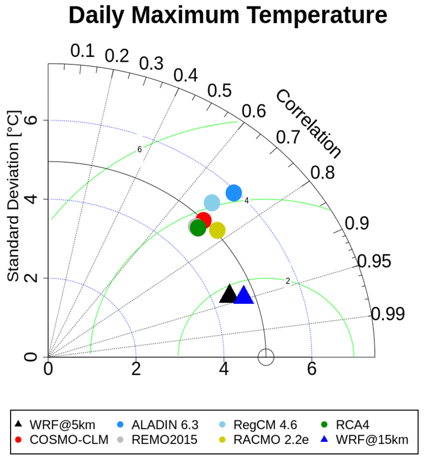
Figure 1 Taylor diagram comparing the model performances in terms of reproducing the daily summer T_max values in relation to the E-OBS reference for the study period 1980–2009 and the whole study area.

Figure 2 Density plot of the summer T_max values from each data set.

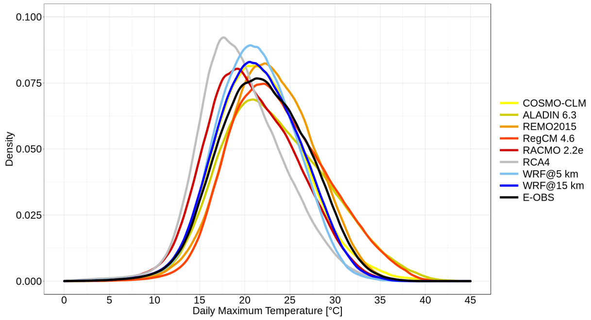
Figure 2 displays a density plot of the summer T_max values from each data set. There are pronounced differences between the single distributions in general, but also at the right tail, which is our focus here. Until approx. 10 ^∘C, all the distributions are relatively similar; the discrepancies begin thereafter. Compared to E-OBS, RCA4 and RACMO are clearly shifted leftwards. Apart from these two models, all the other data sets have most of their values in the range between 20 and 25 ^∘C. ALADIN and RegCM are shifted towards the right compared to E-OBS, especially in the right tail area from approx. 30 ^∘C on, in which they clearly have more values than all the other runs and E-OBS. In this area, REMO shows high agreement with E-OBS, while WRF@5 km and RCA4 have the least amount of values there. The overall differences between the two WRF runs are distinct. The 15 km run is closer to E-OBS than its 5 km counterpart, and it has more values in the right tail of its distribution.

Table 1 gives the bias values of the spatially and temporally averaged maximum temperature values for each RCM. Five runs – COSMO-CLM, RACMO, RCA4 and the two WRF runs – show negative mean bias values; the other runs show positive ones. The highest negative value is found for RCA4 (−2.40 ^∘C), which is also the highest overall value, followed by RACMO (−1.37 ^∘C). This can be inferred from the density plot in Fig. 2. This is also true for the highest positive bias values of ALADIN (1.19 ^∘C) and RegCM (1.62 ^∘C). COSMO-CLM (−0.16 ^∘C) holds the lowest bias value. The overall spread is 4.02 ^∘C (between RegCM and RCA4).

Table 1 Spatially and temporally averaged daily T_max bias values with respect to E-OBS.

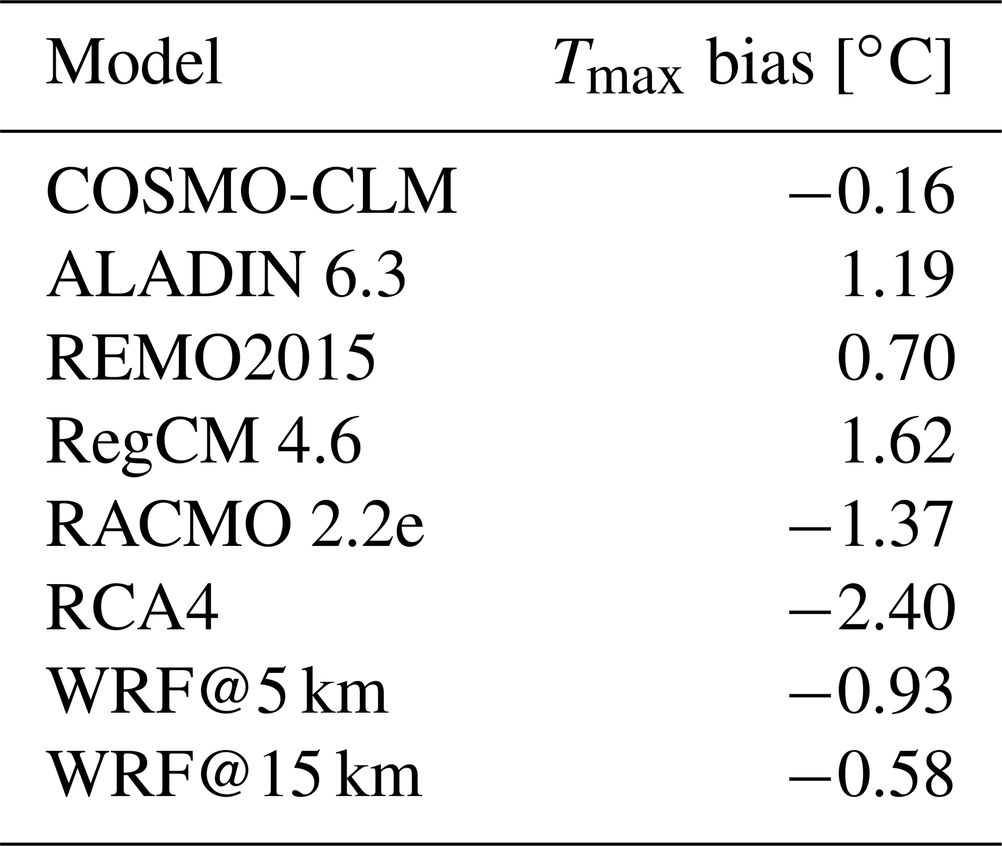
Comparing the outcomes of the Taylor diagram (Fig. 1) with the mean bias values from Table 1 leads to the following insights. ALADIN (1.19 ^∘C), RegCM (1.62 ^∘C) and RACMO (−1.37 ^∘C) hold relatively large mean bias values, while their scores in the Taylor diagram distinctly differ. Here, ALADIN also has a relatively high CRMSE and shows poor agreement with the reference standard deviation, while RACMO shows the lowest EURO-CORDEX CRMSE, high standard deviation agreement, and the highest correlation value out of the EURO-CORDEX RCMs. RegCM also has a low correlation value in the Taylor diagram. COSMO-CLM has the lowest mean bias value (−0.16 ^∘C) and shows the highest agreement with the reference standard deviation in the Taylor diagram. Moreover, it is striking that RCA4 holds the largest mean bias value (−2.40 ^∘C), while it is placed relatively well in the Taylor diagram. It is the opposite case for the WRF outputs. In the Taylor diagram, they show the highest correlation values as well as the lowest CRMSE values, while their mean values in Table 1 are somewhere in the middle. This basically shows that in some cases the individual models have strong or weak values of both terms, while the performances diverge in other cases, meaning that the mean bias values are low but the scores in the Taylor diagram are weak or vice versa. It is important to consider that, for the Taylor diagram, all the grid cell T_max values were used, while in Table 1, as mentioned above, the bias values of the spatially and temporally averaged T_max values are given. Moreover, it needs to be taken into account that any mean bias is implicitly corrected in the CRMSE.

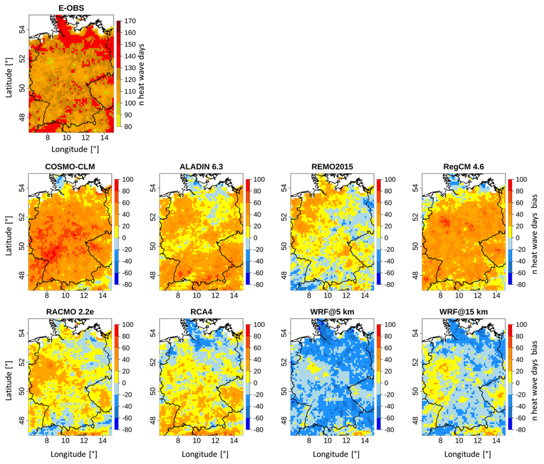
Figure 3 Grid-cell-based E-OBS pattern of the number of heat wave days in the summer months between 1980–2009 and the differences between each RCM and E-OBS.

4.2 Number of heat wave days

Figure 3 presents the E-OBS pattern of the number of heat wave days for the time period 1980–2009 along with the grid-cell-based differences between each RCM and E-OBS. Table 2 provides more detailed information.

Table 2 Metrics for the number of heat wave days.

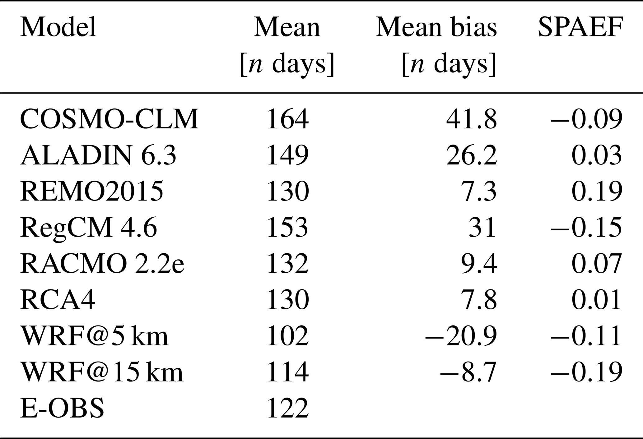
In the E-OBS domain, the highest values are located in the northern, northeastern and southwestern parts, with up to 160 heat wave days. The minimum values range between 80 and 90 d and are sporadically distributed all over the domain. There is no clear area characterized by low values. The domain mean value is 122 d (Table 2). The RCM difference patterns show distinct differences between each other. It is noticeable that some of the domains show either a mostly negative bias (WRF@5 km), which means that they simulated less heat wave days compared to the reference, or a mostly positive bias (COSMO-CLM, ALADIN and RegCM), meaning that they simulated more heat wave days. REMO, RACMO and RCA4 have rather mixed domains. It is striking that the two WRF outputs are the only ones dominated by negative values. The majority of the values across all domains range between −60 and 60 d of difference. COSMO-CLM, ALADIN, RegCM and RACMO have relatively similar bias values in the western parts of the domain. Other than that, there are no repeating patterns across a majority of the RCMs. In the WRF@15 km simulation, there are significantly more positive bias areas compared to its 5 km counterpart, which is also confirmed by Table 2, where the mean bias value of the 15 km run is much closer to 0 (−8.7 compared to −20.9 d). These positive bias areas are mainly located in the western, eastern and southeastern parts of the domain. The values in Table 2 confirm the impressions drawn from Fig. 3: the domain mean values from all the EURO-CORDEX RCMs are above the E-OBS reference value (122 d), with the COSMO-CLM value showing the biggest difference (42 d). The two WRF runs are below the reference (102 and 114 d). The values for REMO and RCA4 (both 130 d) and WRF@15 km come closest to the reference. Regarding the mean bias values, the inferred negative values from the two WRF runs are visible, while the EURO-CORDEX RCMs all show positive mean bias values. COSMO-CLM has by far the highest bias value (41.8 d); REMO shows the lowest value (7.3 d). It should be kept in mind here that for RCMs that are not dominated by one bias direction, the values can cancel each other out, providing a small overall mean bias. This is the case for REMO, RACMO and RCA4. The SPAEF values give information about the pattern agreement between the reference and the individual RCMs (not shown here). There is not a single high value. The values are either negative or very low, meaning that none of the RCMs show good overall spatial agreement with the reference. REMO has the highest value (0.19); WRF@ 15 km has the lowest (−0.19).

There are no apparent benefits of the WRF runs compared to the EURO-CORDEX RCMs. This suggests that neither the increased grid resolution nor the model setup has a decisive effect on the reproduction of the number of heat wave days. In fact, WRF@15 km performed better than its 5 km counterpart, which further underlines that the grid resolution might play a less important role for this aspect. REMO is the RCM with the best overall performance as it has the best values in all regards (Table 2); COSMO-CLM performed the worst.

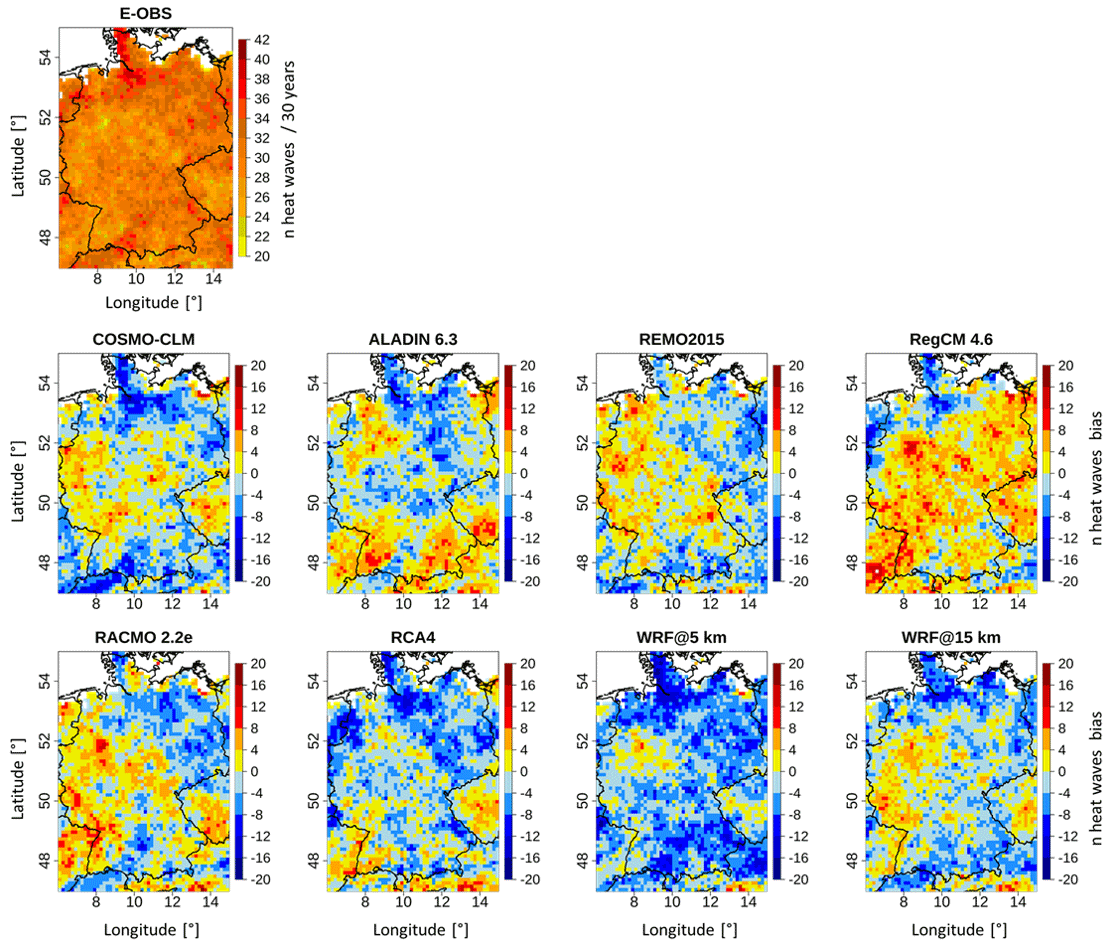
Figure 4 Grid-cell-based E-OBS summer heat-wave frequency pattern between 1980–2009 and the differences between each RCM and E-OBS.

4.3 Heat wave characteristics

4.3.1 Heat wave frequency

Figure 4 shows the E-OBS pattern of the number of heat waves for the time period 1980–2009 and the grid-cell-based differences between it and the RCMs. The relevant scores are given in Table 3.

Table 3 Heat wave frequency metrics.

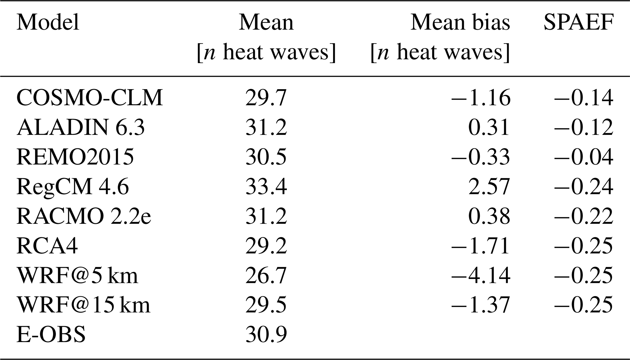
The E-OBS domain looks mostly uniform, with the majority of values ranging between 26–34 heat waves. The domain mean value (30.9) in Table 3 underlines this. Only in the north and south are small concentrations of higher values (up to 40 heat waves). The RCM bias domains show rather mixed patterns with both positive and negative values. RegCM (positive) and WRF@5 km (negative) are the only domains where one bias direction predominates. This is also reflected in the mean bias values in Table 3, where these two RCMs have the highest values (2.57 and −4.14), while the opposite signs tend to cancel each other out in the other domains, bringing them closer to zero on average. In all the bias domains, the northern part is dominated by negative bias values. It is also noticeable that in the eastern part of the domain, only positive values prevail in RegCM, while negative values prevail in all other bias domains in this area. The WRF@15 km experiment looks quite balanced and therefore quite different from its 5 km counterpart. This is also confirmed by the smaller mean bias value (−1.37) in Table 3. The domain mean values in Table 3 show a relatively large range of about seven heat waves between the maximum (33.4 at RegCM) and minimum (26.7 at WRF@5 km) values. The E-OBS reference value of 30.9 means that, on average, there was approximately one summer heat wave per year in the study period. ALADIN and RACMO (31.2) come closest to this value, while WRF@5 km (26.7) shows the biggest discrepancy. COSMO-CLM, REMO, RCA4 and the two WRF runs simulated fewer heat waves on average than the reference, whereas ALADIN, RegCM and RACMO simulated more. ALADIN has the lowest mean bias value (0.31). The mean bias values of COSMO-CLM, REMO, RCA4 and the two WRF runs are negative; the others are positive. All the SPAEF scores between the reference and the single RCM domains (not shown) are negative here, indicating that there is no good overall spatial agreement at all. The highest score (−0.04) is found for REMO and the lowest (−0.25) for RCA4 and the two WRF runs.

There are no recognizable benefits of the two WRF runs either. Here, it is rather the opposite, especially regarding the WRF@5 km run, since it shows the highest mean bias value and the biggest difference to the reference domain mean value in the number of heat waves. In addition, it has the lowest SPAEF value, which is not very meaningful in this case. Clearly, the model settings seem to have a higher importance than the grid resolution. ALADIN showed the best performance in this section, closely followed by REMO.

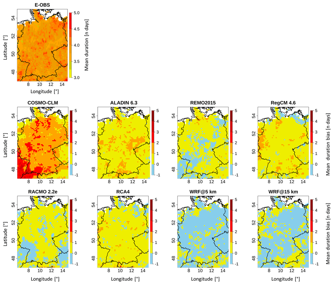
Figure 5 Grid-cell-based E-OBS summer mean heat-wave duration pattern between 1980–2009 and the differences between each RCM and E-OBS.

4.3.2 Mean heat wave duration

Figure 5 displays the E-OBS pattern of the mean heat wave durations for the time period 1980–2009 and the grid-cell-based differences between it and the RCMs. The associated scores are shown in Table 4.

Table 4 Mean heat wave duration metrics.

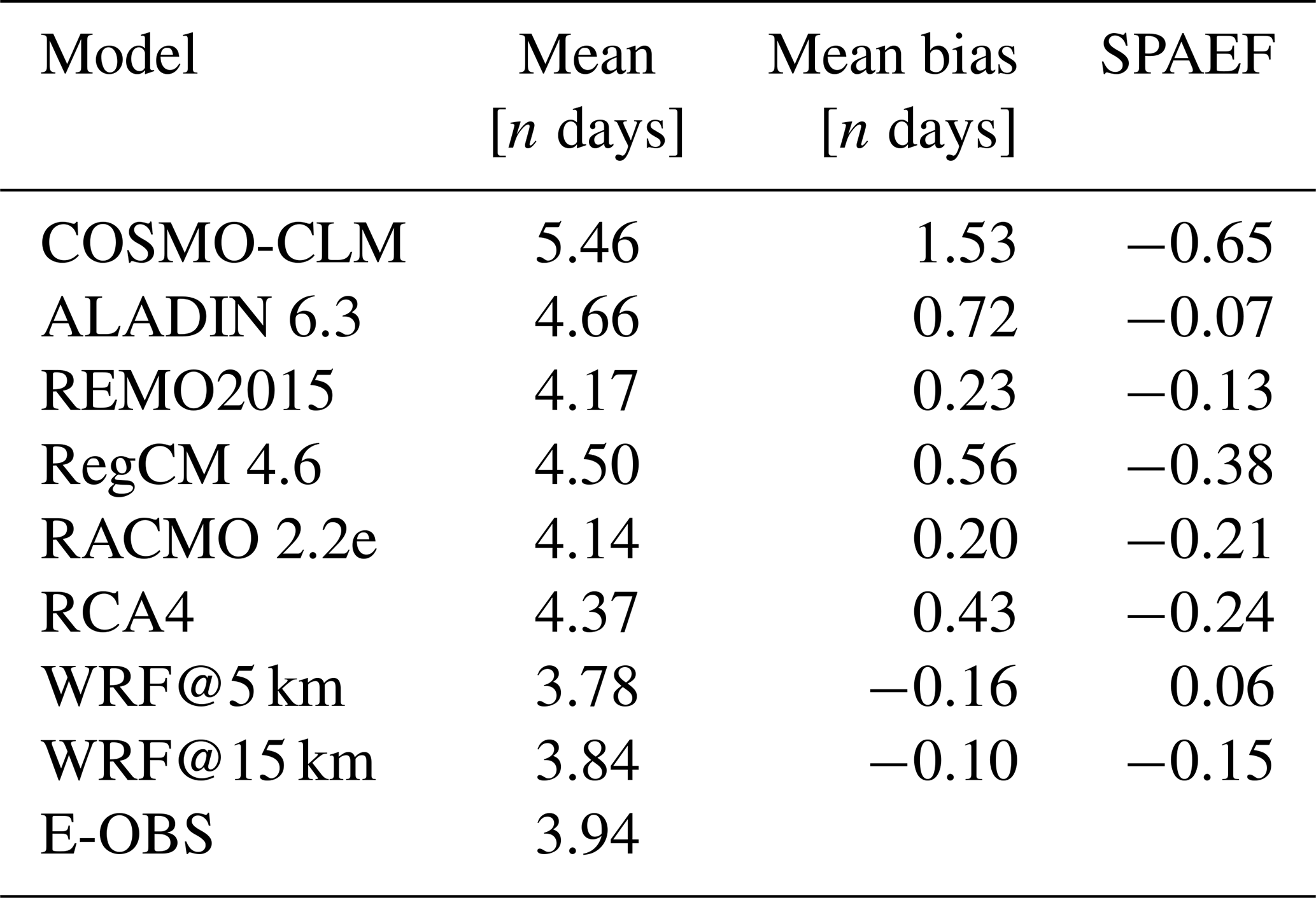
The E-OBS pattern is very uniform; the majority of the domain is covered by values between 3.75 and 4.25 d. This is also reflected in the domain mean value of 3.94 d (Table 4). This means that the average heat wave duration was quite close to the minimum length (3 d) of a heat wave. All EURO-CORDEX RCM bias domains except those for REMO and RACMO are dominated by positive bias values, meaning that the models simulated heat episodes that were too long. The COSMO-CLM domain even appears to lack any cell with negative bias. It is also the domain with the highest values. The area in the southwest, where values of up to 5 d are reached, is especially striking. All other bias domains are dominated by values between −1 and 1 d. The two WRF outputs are the only ones dominated by negative bias values. In this case, the WRF@15 km domain is quite close to its 5 km counterpart, but again the negative bias is less pronounced in direct comparison. The patterns of REMO and RACMO are similar. The domain mean values in Table 4 are all close to each other. All EURO-CORDEX RCMs are above the reference value (3.94 d), while the WRF runs are below it. COSMO-CLM shows the biggest difference (1.52 d), whereas WRF@15 km shows the smallest (0.1 d). COSMO-CLM is also the RCM with by far the highest mean bias value (1.53 d), which was expected based on the bias maps (Fig. 5). It is the only case where the mean bias is greater than 1 d. The bias value of 1.53 d may seem relatively small, but if it is set in relation to the domain mean values, it accounts for a fairly large proportion. Only the two WRF runs have negative mean bias values. WRF@15 km holds the smallest (−0.10) mean bias value. Here, the SPAEF values between the reference and the single RCM domains (not shown) are all negative or very low, which is the case for WRF@5 km (0.06). This means that, again, no RCM was able to satisfactorily reproduce the spatial pattern of the reference. COSMO-CLM also holds the worst value (−0.65) in this regard.

COSMO-CLM is clearly the RCM with the weakest performance due to having the weakest scores in each aspect (Table 4). WRF@15 km is the most reliable RCM here, meaning that there are indeed some benefits of this aspect of the analysis, which are largely related to the model settings, since the 15 km once again performs better than its 5 km counterpart.

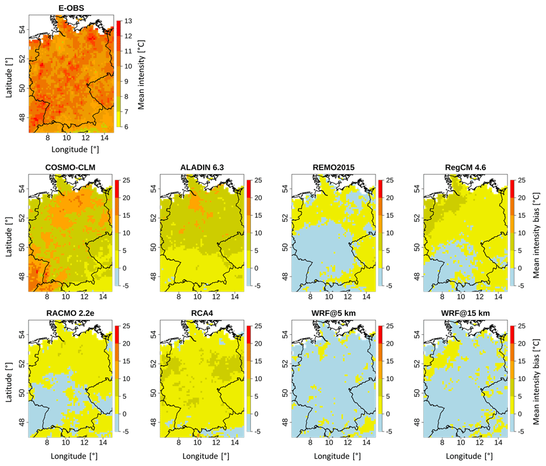
Figure 6 Grid-cell-based E-OBS summer mean heat-wave intensity pattern between 1980–2009 and the differences between each RCM and E-OBS.

4.3.3 Mean heat wave intensity

Figure 6 provides the E-OBS pattern of the mean heat wave intensity for the time period 1980–2009 based on the cumulative heat measure. The grid-cell-based differences between the E-OBS pattern and the RCMs are also included. The relevant scores are given in Table 5.

Table 5 Mean heat wave intensity metrics.

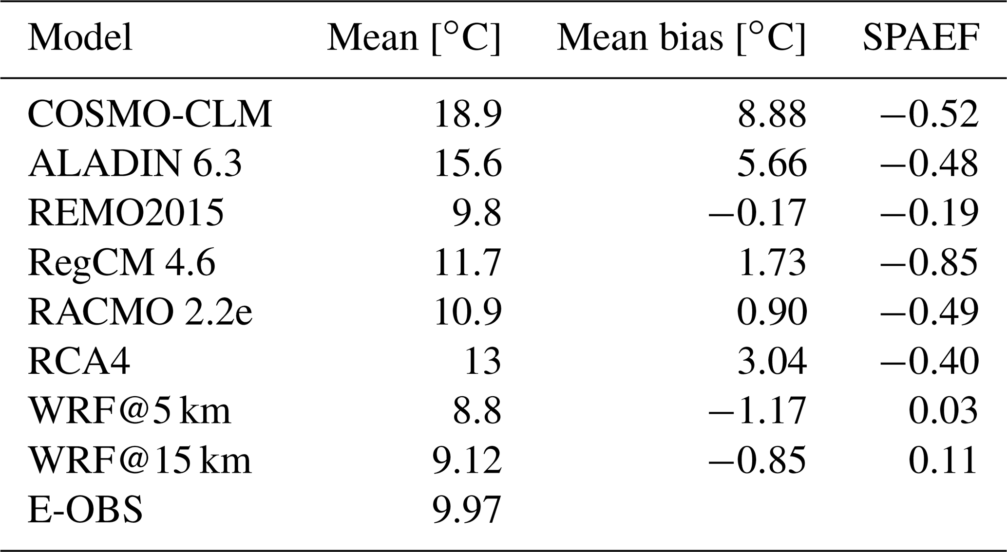
The E-OBS domain looks quite uniform. A sort of band of higher values extends from the southwest to the northeast. The majority of the values lie within 9 to 11 ^∘C, which is confirmed by the domain mean value of 9.97 ^∘C (Table 5). Accounting for the mean duration (3.94 d) of heat waves from the section above, the average heat excess per day during a heat wave period was 2.53 ^∘C. Regarding the RCM bias maps, the two WRF simulations are again dominated by negative values and look quite similar. Areas of positive bias in the 15 km domain are similarly situated to those in its 5 km counterpart. Some of them are more extensive, like those in northwestern part; others are smaller, like those in the southeast. The domains of COSMO-CLM, ALADIN and RCA4 are dominated by positive values, while those of REMO, RegCM and RACMO show a mixed pattern. In those domains, the areas of negative bias are similar; they are mainly located in the southwest. They also have the fact that the values are mostly between −5 and 5 ^∘C in common. This leads to relatively small mean bias values (Table 5) due to mutual balancing. Maximum bias values of up to 25 ^∘C are found at the COSMO-CLM domain in the southwestern part. The COSMO-CLM and ALADIN domains are mainly covered with comparatively high values. The domain mean values in Table 5 show distinct differences, with a maximum range of 10.1 ^∘C between COSMO-CLM and WRF@5 km. The two WRF runs and REMO are below the reference value (9.97 ^∘C), while all the other models are above it. REMO's value (9.8 ^∘C) comes closest to the reference, whereas COSMO-CLM (18.9 ^∘C) shows by far the largest difference – its value is almost double the reference value. As inferred from the maps, REMO and the two WRF runs have negative mean bias values, while the other RCMs have positive ones. REMO holds the smallest value (−0.17 ^∘C) and COSMO-CLM holds the highest, 8.88 ^∘C, which, compared with the domain mean values, is a very high value. The SPAEF values between the reference and each RCM domain (not shown) are, once more, all negative (all EURO-CORDEX RCMs) or very low (the two WRF runs), which means that there is no satisfactory reproduction of the reference's spatial structure. RegCM has the lowest value (−0.85); WRF@15 km has the highest (0.11).

COSMO-CLM is the weakest-performing RCM, while REMO shows the best overall performance. This means that there are no apparent real benefits of WRF here, except for possible minor benefits in relation to reproducing the spatial structure. It is striking that the patterns of the WRF domains are always dominated by negative bias values through all aspects of the heat wave characteristics as well as the number of heat wave days.

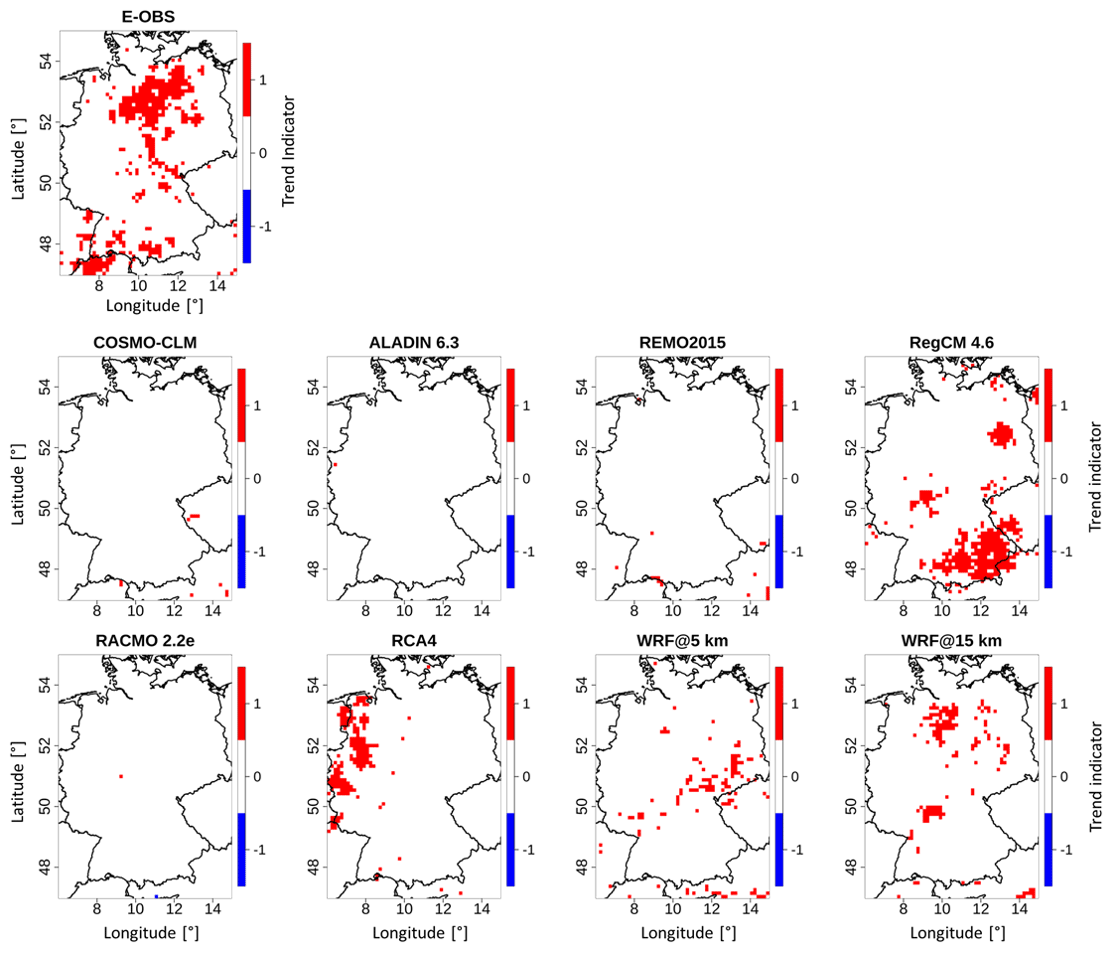
Figure 7 Grid-cell-based trends in the number of annual summer heat waves for 1980–2009 based on the Mann–Kendall test for E-OBS and each RCM.

4.4 Heat wave trends

Figure 7 presents the grid-cell-based results of the Mann–Kendall trend test for the annual number of heat waves in the study period 1980–2009 for all RCMs and the E-OBS reference. A summary of each signal and data set is given in Table 6. In this context, it should be noted that the Mann–Kendall trend test provides information about whether there is a monotonic positive or negative trend or no trend in a time series at a certain level of significance (0.05 here). It does not give information about exact trend values.

Table 6 Metrics for the annual number of summer heat waves overall.

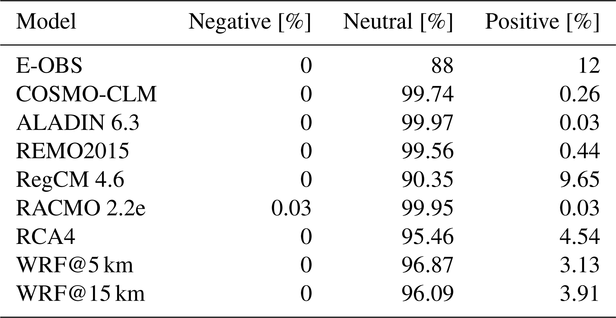
The domains of COSMO-CLM, ALADIN, REMO and RACMO are almost completely covered with no-trend signals. This is confirmed by the values in Table 6, where each of these RCMs has more than 99 % of their grid cells in the neutral section. RegCM and RCA4 have distinct areas of positive trends, but in different areas. WRF@5 km also has positive trend areas, but they are less concentrated. There are also concentrated areas of positive trends in the E-OBS reference domain, mainly in the southwest and in the northern central area. These locations mostly do not agree with those from the RCMs. The WRF@15 km domain also shows positive-trend grid cells, but in different areas compared to the other RCMs. It shows the highest spatial agreement with the reference, especially in the central part. It is striking that there are actually no grid cells with a negative (i.e., decreasing) trend in any domain, which is also confirmed in Table 6. The table further confirms that the majority of the grid cells are covered by no-trend signals. By far the largest proportion of positive grid cells is found for E-OBS (12 %), followed by RegCM (9.65 %), RCA4 (4.54 %) and the WRF runs (3.13 % and 3.91 %). All other runs are in the less than 1 % range. This shows that the WRF@15 km run is closer to the reference than its 5 km counterpart in terms of both the locations and the shares of the signals.

This section reveals that, according to the E-OBS reference, if there is a trend in the number of heat waves, it is only positive, meaning that the frequency is increasing with time. But this is not the case everywhere. All of the models simulate too few pixels with positive trends. Regarding WRF, any possible benefits would be related to the model settings rather than to the grid resolution, since WRF@15 km is more accurate than its 5 km counterpart.

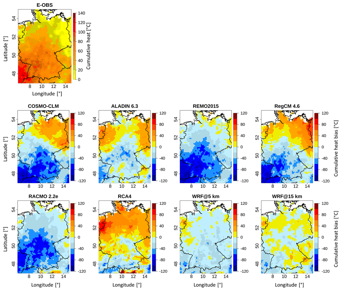
Figure 8 Grid-cell-based E-OBS summer 2003 cumulative heat pattern and the differences between each RCM and E-OBS.

4.5 The 2003 heat wave event

4.5.1 Cumulative heat

Figure 8 shows the E-OBS cumulative heat pattern for the summer season in 2003 and the grid-cell-based differences from each RCM. The associated scores are given in Table 7.

Table 7 Cumulative heat metrics for 2003.

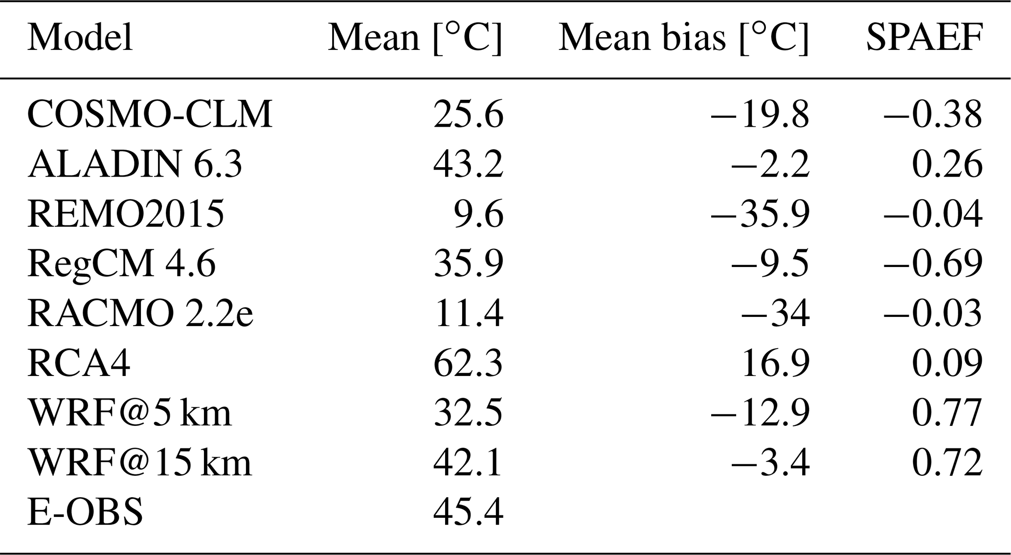
The E-OBS domain shows a quite clear gradient from the southwest to the northeast with decreasing values. The values in the southwest are very high; they accumulated to well above 100 ^∘C during that summer season, making the heat wave most pronounced in this region. These values underline the high intensity of the 2003 heat wave. The mildest values of up to 10 ^∘C heat excess are in the northeastern regions, making them the regions least impacted by the heat wave. COSMO-CLM, REMO, RegCM and RACMO show pronounced negative bias values in the southwest regions of their domains. This means that they were not able to satisfactorily reproduce the particularly high values of the reference in these regions, showing bias values of up to −120 ^∘C. These bias values indicate that the models simulated only weak or even no heat episodes at all in regions where the reference showed the most pronounced values. REMO, RACMO and WRF@5 km are dominated by negative bias values, whereas the remaining RCMs except WRF@15 show mixed patterns where the northern half is dominated by positive bias and the southern half by negative bias, leading to a sort of bipartition. WRF@15 km is evenly covered with positive and negative values. The WRF@5 km pattern is the most uniform one, with relatively low bias values all over the domain. It is striking that, in contrast to the previous sections, the WRF domains are not the only ones dominated by negative bias values here. In direct comparison with its 5 km counterpart, the WRF@15 km domain has many more areas with positive bias. The domain mean values in Table 7 show large discrepancies with each other and a range of 52.7 ^∘C between RCA4 (62.3 ^∘C) and REMO (9.6 ^∘C). The reference value for E-OBS is 45.4 ^∘C. This value is remarkable as it is more than 4 times higher than the mean heat wave intensity (9.9 ^∘C) for the whole study period from Sect. 4.3.3, illustrating the great severity of this heat wave. ALADIN (43.2 ^∘C) is closest to the reference value, while REMO presents the largest difference. Regarding the mean bias values, REMO (−35.9 ^∘C) and RACMO (−34 ^∘C) have the highest values; ALADIN (−2.2 ^∘C) has the lowest. It is important to consider that in the RCMs with the bipartition pattern mentioned above (COSMO-CLM, ALADIN and RegCM), the values cancel each other out, leading to relatively low mean bias values, depending on the degree of balance. Only RCA4 holds a positive mean bias value (16.9 ^∘C). This underlines that the models rather underestimate the intensity of this heat wave period. The mean bias of WRF@5 km (−12.9 ^∘C) is clearly higher than that of its 15 km counterpart (−3.4 ^∘C). Here, there are some distinct differences between the SPAEF values. While they are negative or very low (for ALADIN and RCA4) for most of the EURO-CORDEX RCMs, the two WRF runs show relatively high values (0.77 for WRF@5 km and 0.72 for WRF@15 km). This means that the WRF runs reproduced the spatial structure of the reference reasonably well. RegCM holds the lowest (−0.69) SPAEF value.

There are distinct differences between the individual models in this section. ALADIN is the RCM with the overall best performance; REMO is the one with the worst. Pronounced benefits of the WRF runs are visible in the reproduction of the spatial structure of the reference. In this regard, the 5 km WRF run performs slightly better than its 15 km counterpart. In terms of reproducing the reference domain mean value and in terms of the mean bias value, the 15 km WRF run outperforms its 5 km counterpart.

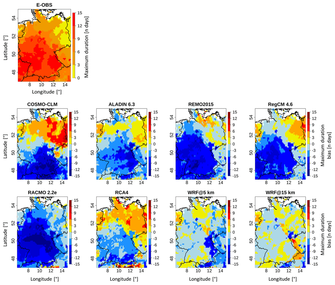
Figure 9 Grid-cell-based E-OBS summer 2003 heat-wave maximum duration pattern and the differences between each RCM and E-OBS.

4.5.2 Maximum duration

Figure 9 gives the E-OBS pattern of the maximum heat wave duration during the 2003 summer season along with the grid-cell-based differences from each RCM. The corresponding values are given in Table 8.

Table 8 Maximum heat wave duration metrics for 2003.

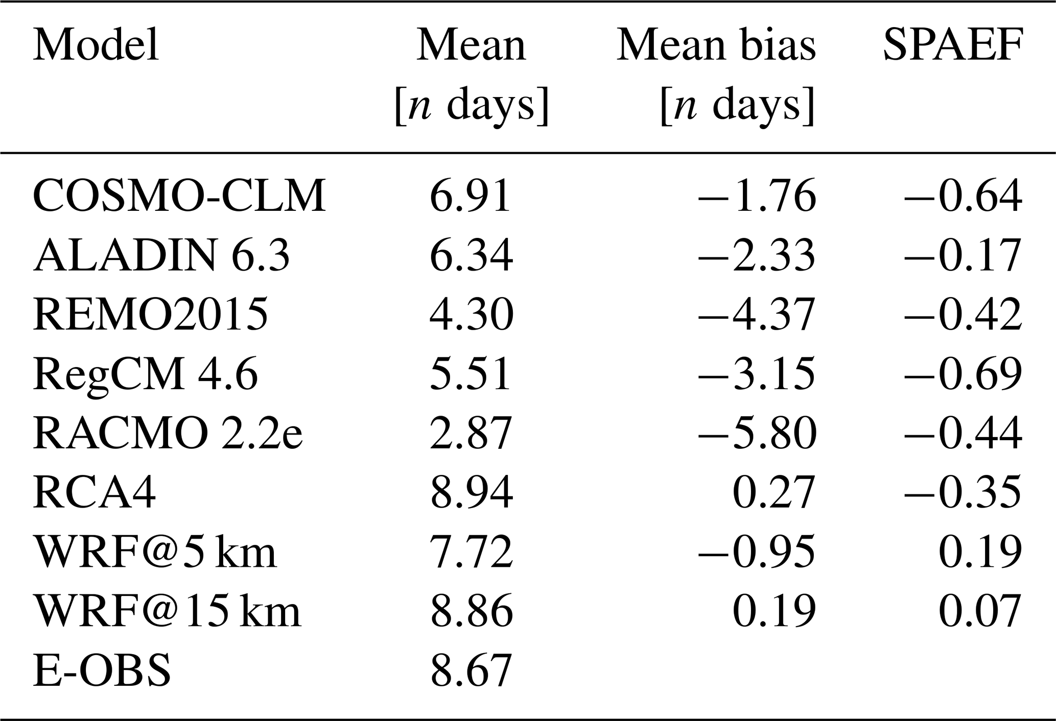
The E-OBS domain shows a sort of bipartition, with the highest values in the southwestern part and lower values in the northeastern part. This matches the impressions gained from the section above, where the highest heat excess values were also found in the southwest (Fig. 8). As the longest durations were up to 16 d, the high heat excess values could accumulate. It should be noted that this is a matter of not only duration but also excess values. In the northeastern part, there are areas with values ranging between 0–3. Since the minimum duration of a heat wave episode was defined to be 3 d, this means that no heat episode took place in these regions in that summer period. This is also in line with the heat excess pattern (Fig. 8), which shows values between 0 and 10 ^∘C in some of these areas. The RCM bias patterns roughly match those in Fig. 8. COSMO-CLM, REMO, RegCM and RACMO have strong negative bias values of up to −15 d in the southern and southwestern areas. Since the E-OBS domain shows the highest values of up to 15 d in some parts of those areas, this further confirms that the models did not simulate a heat wave episode in some parts of these areas where the reference shows the most distinct values. This further underlines this big shortcoming of the models. The northern parts in COSMO-CLM and RCA4 are dominated by positive bias values. COSMO-CLM is the model with the largest areas of high positive bias values of up to 15 d in the eastern parts. This is the region where the E-OBS reference shows only weak or even no heat wave episodes, meaning that the model does the opposite here compared to the southwestern region, simulating relatively strong heat episodes although there were none according to the reference. In almost each domain, there are high bias values in the Alps region in the south. With the exception of RCA4, these bias values are all negative. In line with the section above, the WRF domains are not the only ones dominated by negative values. In the southwestern regions, they both show the lowest bias values of all the RCMs. The WRF@15 km domain shows the most balanced pattern between positive and negative bias values, with most of them ranking in the relatively low range. This is confirmed by the lowest mean bias values (0.19 d) in Table 8. The domain mean values in Table 8 reveal that the E-OBS reference value (8.67 d) is one of the highest; it is only exceeded by RCA4 (8.94 d) and WRF@15 km (8.86 d). This is also reflected in the mean bias values. This indicates that the models tend to simulate shorter durations. The WRF@15 km value is also the closest to the reference, while RACMO (2.87 d) shows the biggest difference. It is also by far the lowest value. The model also holds the highest mean bias value (−5.80 d). It needs to be remembered that the low mean bias values of WRF@15 km and RCA4 (0.27 d) also result from the contradictory nature of their values. Analogously to the cumulative heat, the two WRF runs hold the best SPAEF values (0.19 and 0.07, respectively), but at a much lower level, making them not very meaningful. The score for the WRF@5 km experiment is clearly better than that of its 15 km counterpart. All SPAEF values of the EURO-CORDEX RCMs are negative. The lowest score is found for RegCM (−0.69). Overall, no model reproduces the spatial structures satisfactorily.

According to the scores, WRF@15 km shows the best overall performance in this section; RACMO shows the worst. This means that WRF@15 km outperformed its 5 km counterpart once more. The great weakness of COSMO-CLM, to simulate contrary to the reference, also needs to be considered, since this may not be reflected in the values of the table. The fact that the WRF runs, especially the 5 km run, were not the only models dominated by negative bias values (Figs. 8 and 9) in this section and the previous one, in contrast to what was seen in all the previous sections, highlights that the situation can be very different for a single event compared with the overall picture for the complete study period provided in Sects. 4.2 and 4.3.

4.6 Potential causes of the T_max bias

To investigate potential sources of the bias, we additionally analyzed the following variables from the EURO-CORDEX outputs (the corresponding figures can be found in the Supplement): sensible and latent heat flux, incoming and outgoing shortwave and longwave radiation, soil moisture and surface air pressure. Other outputs from the WRF experiments were no longer available. We performed a correlation analysis (Figs. S1 and S3 in the Supplement) to identify dependencies between the individual predictor variables and T_max for each of the models. The highest T_max correlations were found with the radiation variables, especially with the outgoing longwave radiation. Subsequently, we compared the distributions of the individual variables between the models using boxplots (Fig. S2 and S4). No clear conclusions could be drawn, since the models show quite similar distributions of the variables that show the highest T_max correlations . Exceptions are the sensible heat flux, which does not show a high T_max correlation, and soil moisture. A comparison of soil moisture between the models is not considered useful, since there are considerable differences in the modeled soils, like different numbers of soil layers (e.g., five layers in ALADIN, three layers in RCA4 and four layers in WRF), different layer depths, etc. Anyway, soil moisture does not show high correlations with T_max either. The described procedure was conducted for both the summer months of the entire study period and the summer months of 2003 to ensure that heat wave conditions were included in the analysis. Since the temporal courses of the variables are decisive and the distribution analysis allows only little statements about this, we have additionally looked at the spatially averaged courses of the individual variables in each model run for the summer months of 2003 (Fig. S5). The largest differences between the individual models are also found for the soil moisture here, which is not very meaningful, as already mentioned. Naturally, there is a spread between the single lines for each variable, but they greatly agree in their patterns or variability, respectively, which is more important than the agreement in terms of actual values. The differences that occur in some cases, especially with the radiation variables, as they have the highest correlations, can therefore only provide some degree of explanation, as it is not possible to establish overall consistency with the results. For example, COSMO-CLM, which was shown to overestimate the mean heat wave duration and severity the most (Sects. 4.3.2 and 4.3.3), does not stand out from this perspective. There may be further causes of the biases, e.g., differences in the land-use data of the individual models, but that would go beyond the scope of our study.

5 Discussion

Regarding the T_max reproduction in Sect. 4.1, Silva et al. (2022), who compared monthly T_max values from six historical runs of different GCM-RCM combinations from CORDEX-CORE (with ERA5 used as a reference) for the Pantanal region for the period April–October between 1981 and 2005, found temporally and area-averaged correlation values of between 0.42 and 0.67. These are distinctly less than those seen in our case. The different RCM forcings and the focus on a different period and region must be considered though. As for the bias values (Table 1), in previous studies, a negative bias in the daily T_max was found for the Central European region (Nikulin et al., 2011; Plavcová and Kyselý, 2011). Here, we found both positive and negative bias, depending on the RCM.

Regarding the heat wave characteristics (Sect. 4.3), different reasons for the over- and underestimation by the models have been discussed in the literature. Lhotka et al. (2018b) assume that the overestimation of the heat wave frequency and duration of major heat waves is related to large-scale circulation and soil moisture depletion. The underestimation of these events, on the other hand, is associated with too-moist summertime conditions. Vautard et al. (2013) who, like in the present study, found that simulated heat waves from the EURO-CORDEX RCMs were too long and intense (which was not the case for REMO here), attribute this to biases in the modeled temperature. They state that there “is no clear explanation” for these biases. They suspect that the overestimation of heat waves is connected to a combination of anticyclonic weather and amplifying land–atmosphere feedback. Exaggeration of the land–atmosphere feedback could lead to asymmetry and skewness in the temperature distribution (Jaeger and Seneviratne, 2011), which could stretch temperature values at the extremes and in turn induce higher amplitudes and durations of events. It must be noted that they used the daily mean instead of the maximum temperature for their heat wave definition. Lhotka and Kyselý (2015b) also go in the direction of the land–atmosphere feedback, since they found a connection between heat wave intensity and precipitation during and before these events. Vautard et al. (2013) further found that a coarser resolution led to very persistent heat waves. This is also how it looks if only the WRF@5 km run is compared with the EURO-CORDEX RCMs in the present work. The WRF@15 km run shows that this is related not to the resolution but to setting effects, since it is coarser then the EURO-CORDEX runs. It must be noted that the resolution differences in Vautard et al. (2013) (50 vs. 12.5 km) were much more distinct than in our case. According to Plavcová and Kyselý (2019), an overestimation of circulation supertype persistence may contribute to the development of heat waves that are too long in some simulations. From an overall perspective, the heat wave characteristics, especially frequency and mean duration, are generally quite well captured in terms of spatiotemporal mean values (Tables 3–5). Lin et al. (2022) obtained similar findings, even though they used different heat wave metrics.

As for the 2003 heat wave event (Sect. 4.5), Russo et al. (2016) also found a big discrepancy in the RCM's capability to simulate a single major heat wave event. They attribute this to a model deficiency in simulating really extreme heat waves or to the length of the analyzed time period (1979–2005). This underlines that increasing the resolution does not lead to improved reproduction of severe heat waves in most cases. As an exception, Lhotka et al. (2018a) found exactly that. It must be considered that the difference between the resolutions they compared (12.5 vs. 50 km) was much larger than in our case.

In this context, the role of model internal variability should also be discussed. This has been found to depend on the variable, the season and the domain size. The boundary forcing is weaker in the summer time compared to winter, so that the model is freer to develop its own internal dynamics (Caya and Biner, 2004; Lucas-Picher et al., 2008; Lavin-Gullon et al., 2020). Since only summer periods are regarded in this study, this possibly plays a role in the model performances. Furthermore, the internal variability was shown to play a bigger role for precipitation than for temperature (Giorgi and Bi, 2000; Laux et al., 2017; Lavin-Gullon et al., 2020; Yu et al., 2020). Since it is all about temperature in this study, this fact points towards a smaller role of internal variability. Moreover, it was found that smaller domain sizes are associated with lower internal variability (Giorgi and Bi, 2000; Rinke and Dethloff, 2000; Alexandru et al., 2007; Lucas-Picher et al., 2008; Lavin-Gullon et al., 2020). This is because, in larger domains, the lateral boundary control is reduced due to the large area, so the RCMs have more freedom to develop their own characteristics (Lucas-Picher et al., 2008). This likely plays a role in this study, since there is a crucial difference in domain size between the EURO-CORDEX RCMs and the WRF experiments. The EURO-CORDEX domain is far bigger than the second domain of the WRF experiment, resulting in a higher potential for internal variability. However, since these do not show significantly better performance, the role of internal variability seems to be rather limited. Internal variability is often associated with the successful reproduction of single events (Jain et al., 2023). In this case, it relates to the heat wave event of summer 2003, where the models were shown to struggle with accurate reproduction (Sect. 4.5). This struggle may be partly explained by internal variability. However, it should be noted that the entire summer period of 2003 was considered, with all of its individual heat episodes, as described in Sect. 3.5, which should reduce the role of internal variability. In Sect. 4.3, when reproducing the heat wave characteristics, the summer months for the entire study period were considered, so the values in Tables 3–5 are the overall average values. This should considerably reduce the role of internal variability, as it was shown that it does not affect the domain-wide average climatology (Giorgi and Bi, 2000). The internal variability further depends on the model configuration (Giorgi and Bi, 2000), so that, in this case, it likely varies depending on the model.

In each section of this study, we found an inter-model spread. This is in line with previous heat-wave-related modeling studies, e.g., Vautard et al. (2013), Gibson et al. (2017), Feron et al. (2019), and Silva et al. (2022). Vautard et al. (2013), who also used ERA-Interim-driven EURO-CORDEX outputs, assumed several potential sources of spread: the method used to process boundary conditions in the model, the convection treatment, the different parameterizations, and the way in which the interactions between land surfaces and the atmosphere are accounted for in the models.

In each of the heat-wave-related sections, no evidence was found that an increased resolution leads to better results in reproducing the related metrics. In fact, WRF@15 km always performed better than its 5 km counterpart. This is partly in line with the results of previous studies like Plavcová and Kyselý (2019), in which 25 and 50 km resolution were compared, and Molina et al. (2020) (12.5 vs. 50 km). Cardoso et al. (2019), who also compared 12.5 and 50 km resolution, found a slight benefit of increased resolution. Careto et al. (2022) and Lin et al. (2022) compared 0.11^∘ RCM outputs with the outputs of the driving data at different, much higher, resolutions. In both studies, benefits of the increased resolution were found, particularly for coastal regions. Vautard et al. (2013) (12.5 vs. 50 km) identified some benefits of increased resolution, depending on the aspects of analysis considered. They found that an increased resolution led to reduced biases in the 90th percentile of temperature as well as in the heat wave persistence. Local bias improvements in some coastal regions were also found here. Once more, it is noted that in each of the mentioned studies, the difference between the employed resolutions is much higher than in our case. We assume from our results that a resolution increase from an already relatively high resolution, in this case 12.5 km, has a limited to negligible impact. One aspect that also needs to be considered is the original resolution difference between E-OBS (12.5 km) and WRF@5 km. For certain aspects, structures from E-OBS may be better represented at resolutions closer to it. This could be a reason why the 15 km WRF run in which the other settings are the same performs better. Furthermore, it needs to be kept in mind that in the E-OBS data set, extreme values tend to be smoothed out due to interpolation processes (Haylock et al., 2008; Hofstra et al., 2009). This can mean that, for certain aspects of the analysis where the models showed negative bias, the discrepancy from the true value might be even bigger. Hofstra et al. (2009) emphasize that this effect is more pronounced for precipitation though.

The three RCMs with the best performances overall, especially regarding the reproduction of heat wave characteristics, are ALADIN, REMO and WRF@15 km. COSMO-CLM showed the weakest overall performance. If this is considered, the choice of the parameterization schemes seems to play a minor role, since ALADIN, REMO and WRF have all different schemes for the individual physics. This finding is opposite to that of Davin et al. (2016), who identified the land surface scheme as being highly important for a proper simulation of temperature. The land surface scheme is important for two crucial factors: the soil moisture and leaf area index (LAI). If the LAI within the land-surface model is based on climatological values instead of dynamical calculations, this can increase evapotranspiration and thus lead to a cooling effect, which reduces the maximum temperature values. Another possible determiner of bias is the microphysics scheme, which is responsible for the cloud processes. In earlier studies, the role of cloud cover in (maximum) temperature simulation was highlighted. An increased cloud cover leads to a greater fraction of reflected solar radiation, which in turn leads to a cooling of T_max (Groisman et al., 2000; Sun et al., 2000). Lobell et al. (2007) found that cloud cover is responsible for higher daily T_max variability compared to the daily mean values. They consider the cloud cover to be especially important during the summer period. According to Liang et al. (2008), biases in simulated radiation budgets can lead to errors in surface temperatures. Hamdi et al. (2012) found strong correlations of positive bias with the cloud cover representation. However, since all the models in this study were run with different microphysics schemes (Table 2 in Petrovic et al., 2022), relevant conclusions cannot really be drawn about this. Interestingly, in a study by Lhotka et al. (2018b), COSMO-CLM, used in combination with a driving GCM, was among the RCMs with the best performances in simulating major European heat waves. This could indicate the high importance of the driving data, which is also highlighted by Molina et al. (2020). Moreover, a connection between the T_max bias (Table 1) and the overall performance does not seem to exist, since COSMO-CLM has the lowest mean bias value (−0.16 ^∘C) but the worst overall performance, while RCA4, which holds the highest mean bias value (−2.40 ^∘C), does not show significantly bad performance.

According to Plavcová and Kyselý (2019), biases in the simulations of atmospheric circulation play a crucial role in the simulation of temperature extremes. This is why they claim that an improvement in this field would be among the most important steps in improving the reproduction of extreme temperature events and would thus also lead to more credibility of future projections.

Model forcing also plays a role in the model's performance. As described above, in this case, all model runs had the same ERA-Interim reanalysis forcing. In 2018, the first parts of the successor to ERA-Interim, ERA5, were released by the ECMWF (Hersbach et al., 2020). ERA5 has a finer spatial and temporal resolution, uses a more advanced assimilation system, and includes more data sources. This raises the question of whether model performance could be improved by ERA5 forcing. At the time of the selection of the data sets used in this study, no reanalysis runs driven by ERA5 were retrievable from the EURO-CORDEX platform. In the recent past, there have been a few studies dealing with the comparison of ERA-Interim and ERA5. These studies focus on comparisons of certain variables, such as precipitation (e.g., Nogueira, 2020; Lavers et al., 2022; Steinkopf and Engelbrecht, 2022), or several variables, including precipitation and temperature (e.g., Rakhmatova et al., 2021; King et al., 2022; Nacar et al., 2022) and cloud cover (e.g., Lei et al., 2020), for different parts of the world. In most of the cases, ERA5 performs significantly better than ERA-Interim or contributes to better results. This is especially the case for the reproduction of precipitation. Thus, it is to be expected that the RCM outputs would benefit from ERA5 forcing, leading to better performances. Due to the improvement, especially in precipitation, benefits would likely be more relevant for drought than for heat wave analysis, especially since patterns are better reproduced (Lavers et al., 2022). It may be worth directly comparing simulation outputs from the same RCM driven by ERA-Interim and ERA5. This remains the subject of future studies.

It is striking that there are some significant differences in the outcomes compared to the drought study (Petrovic et al., 2022) in which the same data sources were used as mentioned above. While it was found that all models performed at similar levels for the drought characteristics, there were some significant differences between the individual performances for the heat wave characteristics here, highlighting that the choice of model can be crucial. In addition, it was shown that the WRF settings and increased resolution were particularly beneficial for reproducing drought trends. This is not the case for heat wave trends. This suggests that these benefits are highly related to the simulation of precipitation, the most important variable for drought, which is not a factor here. The different timescales could also be a factor. Unlike heat waves, where the minimum duration in this study is 3 d, droughts are prolonged events with a minimum duration of usually at least 1 month. For this reason, monthly values were considered in the drought study, while daily values were used here. Regarding the reproduction of the 2003 drought and heat wave event, there are pronounced differences between the models in both studies. Interestingly, REMO shows the worst performance in this respect in both cases and significantly underestimates the drought and heat wave conditions, respectively.

6 Conclusions

A heat wave analysis of Germany and its near surroundings for the period 1980–2009 was performed. The impact of an increased model resolution and the appropriate model configuration on the reproduction of heat wave metrics based on T_max simulation was addressed. For this purpose, we employed an ensemble of six ERA-Interim-driven EURO-CORDEX RCMs of 12.5 km horizontal grid resolution as well as outputs of a target-area-tailored, ERA-Interim-driven WRF simulation at 5 and 15 km resolution. The model outputs were evaluated with regard to their ability to reproduce T_max and the heat wave characteristics based on it, trends, and the major event in 2003. E-OBS data were used as reference.

WRF, with its increased resolution and tailored model settings, is not necessarily beneficial to the performance in reproducing heat indices. Only the reproduction of the mean heat wave durations and the spatial structure of the cumulative heat values for the 2003 heat wave event benefits to some extent from the use of WRF. In fact, the WRF@15 km run outperformed its 5 km counterpart in each section. Thus, we can conclude that, for the selected model configurations, increased resolution does not contribute to better performances regarding heat wave metrics when both of the compared resolutions are already relatively high, which was the case here (12.5 vs. 5 km). Since the three models ALADIN, REMO and WRF@15 km show the overall best performances, we further conclude that the tailored model settings of WRF only have limited benefits for the reproduction of the heat wave metrics. The daily T_max values are reproduced relatively well by all models, which is also underlined by the rather low mean bias values in Table 1. Regarding the domain mean conditions of the overall characteristics, all models show reasonable performances for the heat wave frequency and mean duration, while this does not apply to the mean intensity. The spatial agreement with the reference was not satisfactory for any RCM in any section, with the exception of the two WRF runs in the reproduction of the cumulative heat pattern for the 2003 event. In general, despite applying the same forcing by ERA-Interim, the RCMs exhibit a significant spread in their outputs. This is especially pronounced for the 2003 event, which underlines the difficulty in using the models to reproduce single major events. Regarding the heat wave trends, the reference shows that, if there is a trend present, it is only an increasing trend, indicating that the number of heat waves increases with time. The RCMs struggle with reproducing these trends. If trends are indicated, they are mostly not spatially accurate. All RCMs underestimate the proportion of grid cells with increasing trends. No specific physics scheme or configuration was shown to be especially beneficial for the reproduction of the heat wave metrics. Furthermore, there seems to be no correlation between the RCM bias values (Table 1) and the respective RCM performances. According to the E-OBS reference, heat waves occurred about 31 times in the study period, with an average duration of about 4 d and an average intensity of about 10 ^∘C. This equals an average heat excess per day during a heat wave period of about 2.5 ^∘C.

This analysis is a follow-up to our drought study (Petrovic et al., 2022). The two extreme event types, droughts and heat waves, are often considered together and are indeed often, but not always, related. We intended to investigate the same research questions for both events by employing and assessing the same model outputs and by using the same or similar methods to work out commonalities and, above all, differences between these two types of extreme events. In the drought study, it was revealed that all RCMs performed at a similar level in reproducing the drought characteristics based on the domain average, and the WRF experiments showed clear benefits in the trend reproduction. In fact, only WRF was able to reproduce the observed trends to a fairly high spatial accuracy. This was mainly due to the model settings of WRF, but the higher resolution increased the spatial accuracy. In contrast to this, as shown in this study, there are more pronounced differences between the capabilities of the individual RCMs to reproduce heat wave characteristics, so the choice of model is far more important here. Also in contrast to droughts, there are no benefits of WRF in the trend reproduction. What the two studies have in common is that all RCMs were shown to struggle with the reproduction of the single major event of summer 2003. In both cases, there was no model with a satisfying performance in this regard. Increased model resolution and tailored model settings were shown to be more important for drought simulation than for heat wave simulation, especially for trends. This is most likely related to the different variables that play the crucial role in the respective type of extreme event: precipitation for droughts and (maximum) temperature for heat waves.

Our results suggest that a resolution of 12.5 km or even 15 km, as shown by the WRF@15 km run, is sufficient to reach similar findings to those obtained with finer resolutions. Furthermore, it was shown that the model settings that were adjusted to the specific target region of WRF had only limited impacts, suggesting that this is a less important factor in the reproduction of T_max and thus heat waves. The results may guide the selection of suitable RCMs for certain aspects of heat wave analysis in Germany and similar regions – not only in a historical context, but also for future projections.