Modelling crop hail damage footprints with single-polarization radar: the roles of spatial resolution, hail intensity, and cropland density

Hail represents a major threat to agriculture in Switzerland, and assessments of current and future hail risk are of paramount importance for decision-making in the insurance industry and the agricultural sector. However, relating observational information on hail with crop-specific damage is challenging. Here, we build and systematically assess an open-source model to predict hail damage footprints for field crops (wheat, maize, barley, rapeseed) and grapevine from the operational radar product Maximum Expected Severe Hail Size (MESHS) at different spatial resolutions. To this end, we combine the radar information with detailed geospatial information on agricultural land use and geo-referenced damage data from a crop insurer for 12 recent hail events in Switzerland. We find that for field crops model skill gradually increases when the spatial resolution is reduced from 1 km down to 8 km. For even lower resolutions, the skill is diminished again. In contrast, for grapevine, decreasing model resolution below 1 km tends to reduce skill, which is attributed to the different spatial distribution of field crops and grapevine in the landscape. It is shown that identifying a suitable MESHS thresholds to model damage footprints always involves trade-offs. For the lowest possible MESHS threshold (20 mm) the model predicts damage about twice as often as observed (high frequency bias and false alarm ratio), but it also has a high probability of detection (80 %). The frequency bias decreases for larger thresholds and reaches an optimal value close to 1 for MESHS thresholds of 30–40 mm. However, this comes at the cost of a substantially lower probability of detection (around 50 %), while overall model skill, as measured by the Heidke skill score (HSS), remains largely unchanged (0.41–0.44). We argue that, ultimately, the best threshold therefore depends on the relative costs of a false alarm versus a missed event. Finally, the frequency of false alarms is substantially reduced and skill is improved (HSS = 0.54) when only areas with high cropland density are considered. Results from this simple, open-source model show that modelling of hail damage footprints to crops from single-polarization radar in Switzerland is skilful and is best done at 8 km resolution for field crops and 1 km for grapevine.

1 Introduction

Hail storms frequently cause severe damage to agriculture and infrastructure in various places across the globe (Bell et al., 2020; Allen et al., 2020; Gobbo et al., 2021; Rana et al., 2022). In fact, severe convective storms (which include hailstorms) are among the costliest perils worldwide (SwissRe, 2021). Switzerland is a particularly hail-prone country with a nationwide average of 32 hail days during the convective season (April to September) and locally up to 3 or more hail days in hot-spot regions (Schröer et al., 2022). The number of hail days varies strongly from year to year. Summer 2021 was an example of a record hail season, causing extreme damage in a series of intense and widespread thunderstorms (Kopp et al., 2022). The main crop insurer in Switzerland, Schweizer Hagel (SH), reported around 14 000 damage claims and insured losses of around CHF 110 million (approx. USD 117 million; Schweizer Hagel, 2021) for this year. Hail remains the costliest natural hazard for insured agricultural production in Switzerland, and the events of summer 2021 demonstrated the need for reliable assessments of hail risk for key stakeholders including insurers, governments, and farmers.

Compared to other weather-related hazards, reliable data on hail remain scarce due to the small scale of thunderstorms and accompanying hail streaks as well as the high costs to maintain observational networks at a large scale. Therefore, radar data are frequently used to obtain an estimate of hail on the ground because they are continuous in space and time (Kunz and Kugel, 2015; Puskeiler et al., 2016). Recently, the Swiss Federal Office of Meteorology and Climatology (MeteoSwiss) has compiled a comprehensive assessment of hail frequency and hail stone sizes for Switzerland based on 20 years of single-polarization radar data at 1 km spatial resolution, providing an important basis for hail risk assessments (Schröer et al., 2022; Trefalt et al., 2022). The climatology is based on two hail products that are computed operationally: the Maximum Expected Severe Hail Size (MESHS), which is different from the widely used Maximum Expected Size of Hail (MESH; Witt et al., 1998), and the Probability of Hail (POH; Betschart and Hering, 2012). Both are based on a height difference between the melting level and the height of a given reflectivity level, a criterion introduced by Waldvogel et al. (1979). MESHS and POH are physically meaningful as they relate to the vertical extent of the thunderstorm updraught above the melting level, representing the hail growth zone. A larger vertical extent is associated with a higher likelihood of hail as well as an increase in the potential size of hailstones.

Single-polarization radar products such as MESHS and POH provide valuable estimates of the occurrence of hail on the ground as verified with, for example, insurance claims (Holleman et al., 2000; Kunz and Kugel, 2015; Puskeiler et al., 2016; Nisi et al., 2016), reports of observers and media (Cică et al., 2015), and crowdsourced hail reports (Barras et al., 2019). Verification based on insurance claims generally shows a high probability of detection (POD, fraction of damage events that is predicted, often around 0.8 or larger) but also a relatively high false alarm ratio (FAR, fraction of predictions without damage, up to 0.8) (Kunz and Kugel, 2015; Puskeiler et al., 2016; Nisi et al., 2016; Warren et al., 2020; Schmid et al., 2024). However, these metrics usually strongly depend on the hail intensity threshold used to identify damaging hail, the objective selection of which is not always possible. For example, one can choose the threshold with the highest skill score (e.g. Puskeiler et al., 2016) or one can require that frequency of damage prediction equals the frequency of damage occurrence (i.e. a frequency bias of 1; Warren et al., 2020). Further, these verification studies usually rely on pragmatic choices regarding the scale of spatial aggregation or the distance between damage claim and radar signal tolerated. One reason for this is that insurance claims are often only available at the municipality level, which is typically much coarser than the resolution of the radar observations (∼ 1 km). A strong dependence of the skill on the spatial scale can be expected, as lowering the spatial resolution (or increasing the tolerated distance between damage claim and radar signal) increases the likelihood of overlap between radar signals and damage (Holleman et al., 2000; Schmid et al., 2024). The physical reasons for this are the horizontal drift of hail by wind (e.g. Schiesser, 1990) and limitations in the spatial accuracy of radar-based hail observations, which rely on storm-related proxies to infer hail sizes on the ground (Betschart and Hering, 2012). Also, information on the presence and density of exposed assets (e.g. buildings, cars, cropland) is essential for reliable skill metrics but has often not been incorporated in previous verification studies.

Early efforts to relate crop damage to radar information (Omoto and Seino, 1978; Seino, 1980; Schiesser, 1990) or to hail pad measurements (Changnon, 1971; Morgan, 1976; Katz and Garcia, 1981) derived crop-specific damage functions based on data pairs of damaged fields and observed measures of hail intensity. Schiesser (1990) presented damage functions that link harvest loss at the field scale for individual crop types at various phenological stages to hail kinetic energy derived from single-polarization radar. Sánchez et al. (1996) developed a statistical model to estimate harvest loss for barley and wheat based on hail sizes observed by hail pads and meteorological observers in north-western Spain. More recent efforts used satellite imagery to estimate crop damage after a hail event (Bentley et al., 2002; Singh et al., 2017; Prabhakar et al., 2019; Bell et al., 2020; Sosa et al., 2021).

Despite past efforts to quantify hail damage to specific crops, there is (to our knowledge) a lack of openly available models for assessing crop hail damage. Existing models have been developed in the insurance industry and are proprietary (AIR Worldwide, 2023). Here, we present an open-source model to predict hail damage footprints to field crops and grapevine in Switzerland based on operational radar data and detailed information on agricultural land use. The model is verified with geo-referenced damage claims from SH. To make it accessible to stakeholders, the model is implemented in the open-source natural catastrophe modelling platform CLIMADA (CLIMate ADAptation) (Aznar-Siguan and Bresch, 2019).

To extend the CLIMADA platform with a hail damage footprint detection module, in this study hail intensity measures from operational, single-polarization radar (MESHS and POH) are combined with detailed, crop-specific, geo-referenced cropland information to build simple yes/no damage models for field crops (wheat, corn, barley, rapeseed) and grapevine at different spatial resolutions. The models are systematically verified based on detailed, crop-specific damage information from SH of 12 recent hail events in Switzerland.

More specifically, the following questions are addressed:

1. What spatial resolution is most suitable to model hail damage footprints for field crops and grapevine based on operational, single-polarization radar data in Switzerland?

2. Is it possible to objectively define the best MESHS and POH threshold(s) to model hail damage footprints?

3. How sensitive is the model performance to cropland density?

While most of the study focuses on MESHS, the same methodology is also applied to POH, and results are compared.

The remainder of this paper is structured as follows. First, the three main datasets are introduced and the model setup and verification method described (Sect. 2). Then, how the model skill depends on spatial resolution (Sect. 3.1) and MESHS threshold (Sect. 3.2) is discussed. Subsequently, the combined effect of threshold and resolution is analysed (Sect. 3.3). The sensitivity of this combined effect to cropland density and the use of POH as a hazard variable is then assessed in Sect. 3.4. Finally, the key results are discussed, including how the use of alternative verification approaches might affect them (Sect. 3.5). The paper ends with a summary of the key conclusions in Sect. 4.

2 Data and methods

2.1 Hail hazard data

In this study, single-polarization radar data products on a 1 km × 1 km regular grid are used to quantify hail intensity. The Swiss radar network consists of five dual-polarization Doppler C-band radars (black dots in Fig. 1) and has been in place in this form since 2016 (Germann et al., 2016). The two products used here, the Maximum Expected Severe Hail Size (MESHS) and the Probability of Hail (POH), are computed operationally by MeteoSwiss (Betschart and Hering, 2012; Trefalt et al., 2022; Germann et al., 2022). The underlying reflectivity data are mapped to a regular 1 km × 1 km grid using a pre-calculated projection table relating polar to Cartesian coordinates. Reflectivity is calibrated with multiple independent sources of information, including various types of weather echoes, ground clutter, signals from the sun, and others (Germann et al., 2015). Radar signal attenuation can lead to a bias in individual hail cells, but we expect this bias to be small compared to the known inherent uncertainty of hail detection from radar data, which is due to the indirect estimation of hail size. Note that direct hail size estimation is limited by resonance scattering effects in large hail stones (e.g. Kaltenboeck and Ryzhkov, 2013). MESHS describes the empirical relationship between the size of the largest hailstone and the difference between the top of the 50 dBZ echo and the freezing level height. It is computed from the so-called “Treloar nomogram” of Joe et al. (2004), which is based on Treloar (1998). MESHS ranges from a minimum value of 20 mm to, theoretically, no upper limit. Note that MESHS is designed to indicate the size of the largest hailstone within 1 km² and does not represent a spatial average. Although it is not explicitly connected to actual hail size, positive relationships between MESHS and crowdsourced hail sizes have been reported by Barras et al. (2019). Here, daily (06:00–06:00 UTC) maximum MESHS values are used to define a hail day (or hail event). We use 06:00 UTC (08:00 local time) to define a hail day because it represents the minimum of the average daily hail activity (Schröer et al., 2022). This minimizes the risk of splitting a single hail event into 2 consecutive hail days.

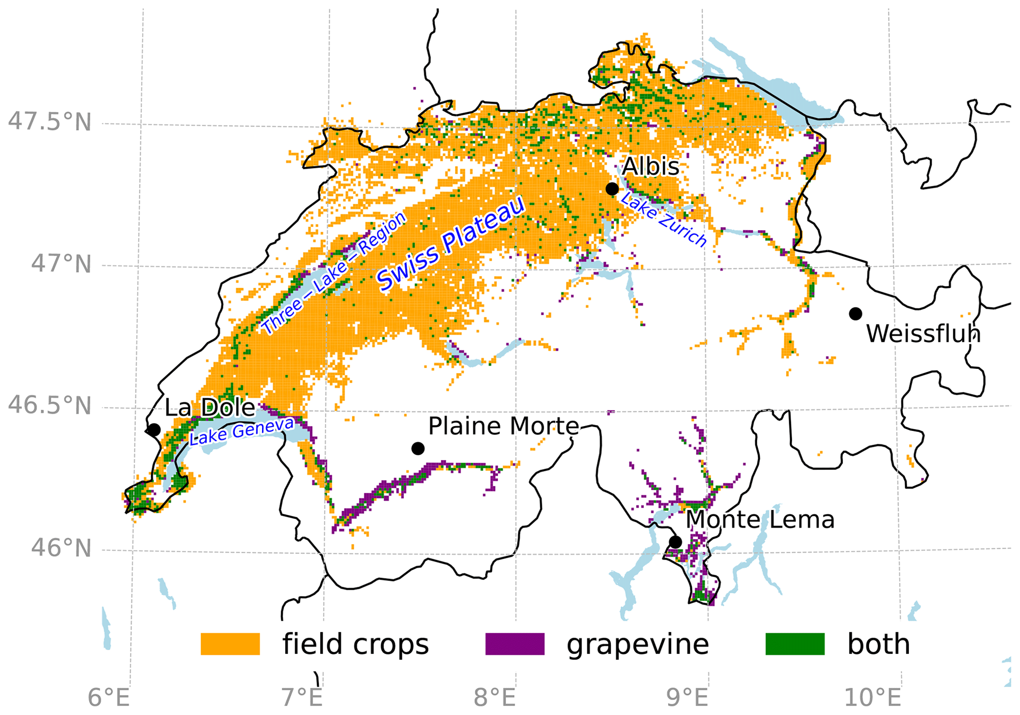
Figure 1 Study region showing exposed field crops (orange), grapevine (purple), and both of the two categories (green), at 1 km resolution with at least one field per square kilometre, and the five radar locations (black dots). Regions and lakes appearing in the discussion of the results are named in blue.

POH is based on an empirical relationship between the likelihood of hail at the ground and, similar to MESHS, the height difference between the top of the 45 dBZ echo and the environmental freezing level. It was originally introduced by Waldvogel et al. (1979) and further developed by Witt et al. (1998) and Foote et al. (2005). The form of the relationship by Foote et al. (2005) has been used operationally by MeteoSwiss since 2008 (Trefalt et al., 2022). As for MESHS, daily (06:00–06:00 UTC) maximum values are used.

To investigate how the model skill changes with reduced spatial resolution, the radar data (MESHS and POH) are aggregated at 2, 4, 8, 16, and 32 km spatial resolution using the maximum value within each grid cell. The maximum is preferred over the mean because it largely conserves the value range of MESHS and POH. Further, this approach is consistent with the assumption that the maximum intensity value determines the occurrence of damage.

2.2 Agricultural exposure data

Detailed geospatial information on agricultural production was obtained from official Swiss land use data (geodienste.ch, 2022). The data are available only starting from 2021, which we use here as a reference. The original data contain polygons of each agricultural field and information on its type of use and cultivated crop. For this study, the data are aggregated to the number of fields and the total crop area within a 1 km × 1 km grid for winter wheat, maize (including silage and forage maize), winter barley, rapeseed, and grapevine, based on the centre point of each field. Further, an aggregate category called field crops is defined that incorporates winter wheat, maize, winter barley, and rapeseed. To model hail damage footprints at the grid scale, these exposure data are converted into a binary field depending on the number of fields n within a grid cell.

$$\begin{array}{}\text{(1)}& \text{exposure}=\left\{\begin{array}{ll}\mathrm{0}& n<n_{\text{thresh}}\\ \mathrm{1}& n\ge n_{\text{thresh}}\end{array}\right.\end{array}$$

If not specified otherwise, n_thresh is set to 1. This means that a grid cell is included as exposure if it contains at least one field of the considered crop type (shown for field crops and grapevine in Fig. 1). Because it is expected that the probability of damage increases with n_thresh, the sensitivity of the model skill to different choices of n_thresh is examined in Sect. 3.4. Cropland density can be expressed as the number of fields per square kilometre (cropland number density, shown in Fig. A1) or, since the area of each field is known, as the fraction of land area covered by a specific crop (cropland area fraction). For n_thresh=1 and 1 km spatial resolution, the average cropland densities (in grid cells where the crops are present) are 36.7 (grapevine), 9.7 (field crops), 4.6 (wheat), 4.3 (corn), 2.5 (barley), and 2.4 (rapeseed). The corresponding cropland area fractions are 7.3 % (grapevine), 14.4 % (field crops), 5.7 % (corn), 3.5 % (barley), and 4.2 % (rapeseed). The gridded cropland data (number of fields, total area) are provided open-source via the CLIMADA application programming interface (API).

2.3 Model formulation

The model formulation evaluated here follows the risk framework of the IPCC (IPCC, 2022) implemented in CLIMADA (Aznar-Siguan and Bresch, 2019) and defines a hazard, exposure, and an impact function. The impact function describes the vulnerability of exposed assets to the hazard. Here, the exposure consists of a binary field and the hazard consists of the radar data (MESHS). The impact function is defined by one threshold parameter s and represents a step function, which is 0 below s and 1 above s.

$$\begin{array}{}\text{(2)}& f_{\text{imp}}=\left\{\begin{array}{ll}\mathrm{0}& \text{MESHS}<s\\ \mathrm{1}& \text{MESHS}\ge s\end{array}\right.\end{array}$$

The impact, i.e. the damage footprint, is then computed as the product of exposure and impact function.

$$\begin{array}{}\text{(3)}& \text{impact}=\text{exposure}\cdot f_{\text{imp}}\end{array}$$

The resulting impact is a binary field with 1 for grid cells where there is modelled damage and 0 where there is not.

2.4 Damage claims

To evaluate the skill of this model, damage information is obtained from claims data provided by the Swiss Hail Insurance Company (SH) for 10 hail events between 2017 and 2021. Damage information includes the event date, location, crop type, and harvest loss as estimated by employees of SH in the field. Roughly a quarter of all claims indicated zero harvest loss and were removed. This resulted in a total of 26 292 crop-specific damage claims used for this study, out of which 21 % are winter wheat, 26.5 % maize, 10 % rapeseed, 8.5 % winter barley, and 34 % grapevine. About 76 % of these claims contain explicit coordinates of the affected fields, while the remaining claims are only provided at the municipality level. To still be able to consider them in our analysis, these remaining claims are randomly distributed on all farmland (wheat, maize, barley, rapeseed) or all vineyards (grapevine) of that community. This procedure was repeated 1000 times for wheat and grapevine to assess the uncertainty associated with this random placement. It was found that the 95 % confidence interval for the skill metrics considered in this study at 1 km spatial resolution is below 1 % for wheat and below 2 % for grapevine. Therefore, the uncertainty introduced by the random placement is considered small.

Table 1 Overview of the 12 investigated hail events.

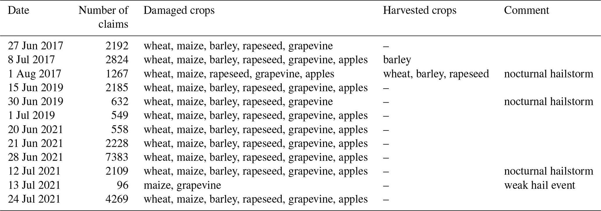
Based on a careful comparison with radar data and the Swiss Severe Weather Database (sturmarchiv.ch, 2024), some damage claims related to nocturnal hailstorms were re-dated to the previous day to match the time window of the radar data (06:00–06:00 UTC). This resulted in a total of 12 hail days (see Table 1) instead of the 10 hail days provided in the original data by SH. Two of the hail events (8 July 2017 and 1 August 2017) occurred when at least one of the crops had already been completely or largely harvested. These dates were identified by comparing the number of reporter damage claims for the various crops (no or only a few claims for a crop but many claims for the other crops) (see fourth column in Table 1). These dates were further verified based on information on indicative starting dates for harvests (wheat: end of July; barley: end of June; rapeseed: mid-July; maize: October) (Schweizer Bäuerinnen und Bauern, 2023).

Finally, to allow damage to be compared directly to exposures and modelled damage footprints, damage claims were gridded to the same 1 km × 1 km grid as the exposure data. This gridded dataset indicates the number of damaged fields separately for each crop type as well as the aggregate field crops category. It is important to note that, in Switzerland, average insurance coverage is 69 % for field crops and 43 % for grapevine (SH, personal communication), indicating that, in our study, the total number of damaged fields is probably underestimated. This is expected to negatively affect model skill, mainly via a larger number of false alarms.

Damage and exposure data are from different sources, and therefore whether damage actually occurs where exposure is identified is checked. The fraction of claims that are in a 1 km × 1 km grid cell without exposure is small (wheat: 3 %; corn: 2 %; barley: 7 %; rapeseed: 11 %; field crops: 0.5 %; grapevine: 0.4 %) and decreases strongly for coarser resolutions. For the aggregate category field crops, the mismatch is significantly lower than for the individual crops. The more relevant number for our study is the fraction of grid cells with damage that have zero exposure because such grid cells would artificially reduce model skill. This fraction is larger but remains in the range of a few percent (wheat: 5 %; corn: 4 %; barley: 9 %; rapeseed 13 %; field crops: 1.5 %; grapevine: 4 %) and also decreases for coarser resolutions, reaching almost zero at 8 km for all field crops and about 2 % for grapevine. Hence, a coarser resolution can efficiently reduce the mismatch between damage and exposure, in particular for field crops. Note that the exposure used here is in principle only valid for 2021. However, there are only small differences in the mismatch between events in 2021 and events prior to 2021, indicating that this is not a major source of uncertainty. To avoid artificially reducing the skill of the model due to the (albeit small) mismatches, grid cells with damage but no exposure are excluded from the verification process. The gridded damage data (number of fields) are provided open-source via the CLIMADA data API.

2.5 Verification based on contingency table

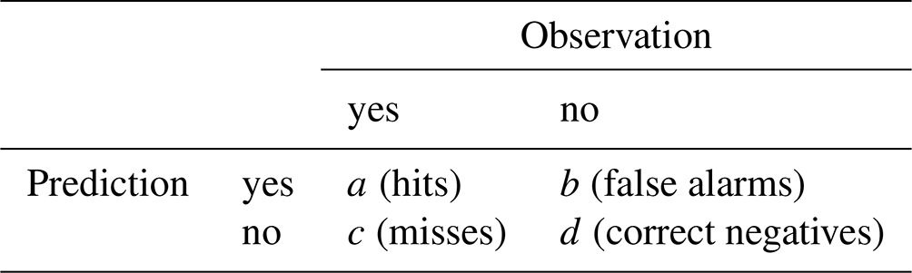
To measure the model skill at different spatial resolutions and for different MESHS or POH thresholds, we use a 2 × 2 contingency table computed based on the joint distribution of predictions and observations on all grid cells with non-zero exposure (Table 2; cf. Wilks, 2019). According to the model formulation, grid points with non-zero exposure that coincide with a hail intensity larger than a threshold s are considered damage predictions (a+b in Table 2). Grid points with non-zero damage and non-zero exposure are considered damage observations (a+c in Table 2). From the four numbers of the contingency table (a is hits; b is false alarms; c is misses; d is correct negatives), a range of scalar attributes and skill metrics are computed (Wilks, 2019).

$$\begin{array}{ll}{\displaystyle }& {\displaystyle }\text{FAR}={\displaystyle \frac{b}{a+b}}\text{POD}={\displaystyle \frac{a}{a+c}}\\ {\displaystyle }& {\displaystyle }\text{FB}={\displaystyle \frac{a+b}{a+c}}={\displaystyle \frac{\text{POD}}{\mathrm{1}-\text{FAR}}}\text{PC}={\displaystyle \frac{a+d}{a+b+c+d}}\\ {\displaystyle }& {\displaystyle }\text{CSI}={\displaystyle \frac{a}{a+b+c}}={\displaystyle \frac{\mathrm{1}}{\frac{\mathrm{1}}{\mathrm{1}-\text{FAR}}+\frac{\mathrm{1}}{\text{POD}}-\mathrm{1}}}\\ {\displaystyle }& {\displaystyle }{\mathrm{PC}}_{\mathrm{rand}}={\displaystyle \frac{(a+b)(a+c)+(b+d)(c+d)}{(a+b+c+d{)}^{\mathrm{2}}}}\\ {\displaystyle }& {\displaystyle }\text{HSS}={\displaystyle \frac{\text{PC}-{\mathrm{PC}}_{\mathrm{rand}}}{\mathrm{1}-{\mathrm{PC}}_{\mathrm{rand}}}}={\displaystyle \frac{\mathrm{2}(ad-bc)}{(a+c)(c+d)+(a+b)(b+d)}}\end{array}$$

Here FAR denotes the false alarm ratio, POD the probability of detection or hit rate, FB the frequency bias, PC the proportion correct (also called accuracy), CSI the critical success index (also known as threat score), and HSS the Heidke skill score. For a perfect model, FAR is 0 and all other metrics 1, with an FB > 1 indicating over-forecasting and FB < 1 under-forecasting. PC and CSI are both measures of forecast accuracy, but CSI has the advantage that it is a simple measure to account for the trade-off between high POD and low FAR (Roebber, 2009). However, PC has the advantage over CSI in that it takes into account the ability of the model to correctly predict non-events (correct negatives, d in Table 2). The HSS is a classical forecast skill score and quantifies the PC of the forecast compared to the PC of a random forecast, PC_rand (perfect model: HSS = 1; no skill: HSS = 0; Heidke, 1926). The overall model performance in this study is assessed based on the HSS. For comparison, prior studies achieved an HSS of radar-based hail detection around 0.3–0.5 (e.g. Kunz and Kugel, 2015; Ortega, 2018; Warren et al., 2020), with Warren et al. (2020) regarding their values around 0.5 as “moderate skill”.

Table 2 The 2 × 2 contingency table.

3 Results

3.1 The effect of resolution on model skill

First, average model skill as measured by HSS across all events and its dependence on spatial resolution is investigated for each crop type individually for a MESHS threshold of s = 20 mm (Fig. 2). For wheat, maize, rapeseed, and barley, model skill substantially increases with decreasing spatial resolution up to 8 km and decreases or remains constant for coarser resolutions. Aggregating them to one crop type (field crops) conserves this behaviour but increases overall skill. For grapevine, the behaviour is opposite: skill reduces with decreasing resolution up to 8 km and increases again thereafter. The increased skill when verifying hail damage on a larger scale is well known for neighbourhood-based approaches (Warren et al., 2020; Schwartz, 2017; Schmid et al., 2024), even if these approaches have substantial methodological differences from our resolution-based approach. It can essentially be explained by the reduced penalization of forecasts due to spatial displacement from the observation (hereafter referred to as the scale effect). However, the reduced skill with coarser resolution for grapevine cannot be explained with the scale effect.

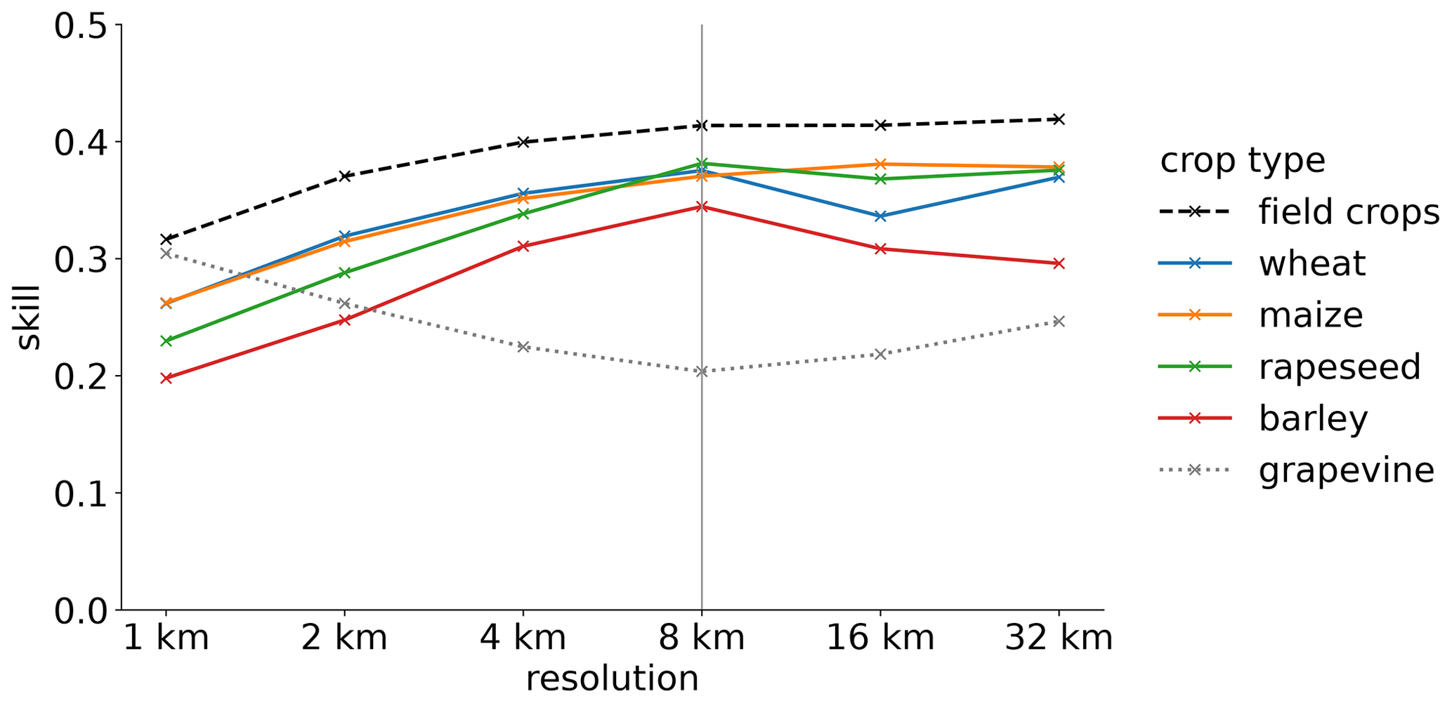
Figure 2 Skill (HSS) of the prediction of hail damage footprints with MESHS (20 mm threshold) for wheat (blue), maize (orange), rapeseed (green), barley (red), and grapevine (dotted grey), as well as the aggregate class field crops (dashed black, includes wheat, maize, rapeseed, barley), as a function of spatial resolution.

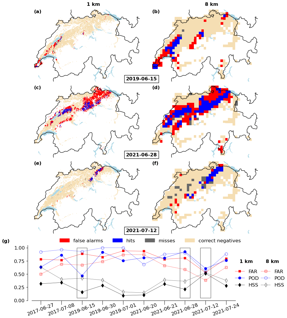
Figure 3 (a, c, e) 1 km × 1 km and (b, d, f) 8 km × 8 km grid cells classified as false alarms (red), hits (blue), and misses (grey) for damage to wheat based on MESHS > 20 mm. Dates shown are (a, b) 15 June 2019, (c, d) 28 June 2021, and (e, f) 12 July 2021. Unshaded cells indicate grid cells without exposure. (g) FAR, POD, and HSS for all 10 recorded events and for (filled symbols) 1 km spatial resolution and (empty symbols) 8 km spatial resolution. Black boxes in panel (g) indicate the events shown in panels (a–f).

To further explore this contrasting behaviour, the effect of resolution on model skill is considered for individual events for both wheat (Fig. 3) and grapevine (Fig. 4) with s = 20 mm. Focusing on wheat at 1 km (Fig. 3a, c, e, and g), high average POD and FAR (both around 0.8) are found, with considerable differences between events. We discuss three representative examples (a shifted forecast, an over-forecast, and a good forecast) in more detail. An event with low skill (HSS = 0.16, POD = 0.47, FAR = 0.89) occurred on 15 June 2019 over western Switzerland (Fig. 3a). In this case, the observed damage footprint (grey and blue grid cells) is shifted to the east relative to the predicted damage footprint (red and blue grid cells), resulting in many misses and false alarms and few hits. Then, 28 June 2021 (Fig. 3c) was an extreme hail event with an exceptionally large spatial extent (Kopp et al., 2022) (HSS = 0.21, POD = 0.91, FAR = 0.81). It is characterized by many false alarms, notably over north-eastern Switzerland. This results in low skill despite the high POD. With a large frequency bias (FB = 4.8) this forecast can be characterized as over-forecast. Finally, the event on 12 July 2021 (Fig. 3e) has the best skill (HSS = 0.51, POD = 0.61, FAR = 0.53). The main damage footprint over north-eastern Switzerland was captured very well, but a number of misses at the edges of the damage footprint and scattered over the Swiss Plateau leads to a lower POD compared to the previous example.

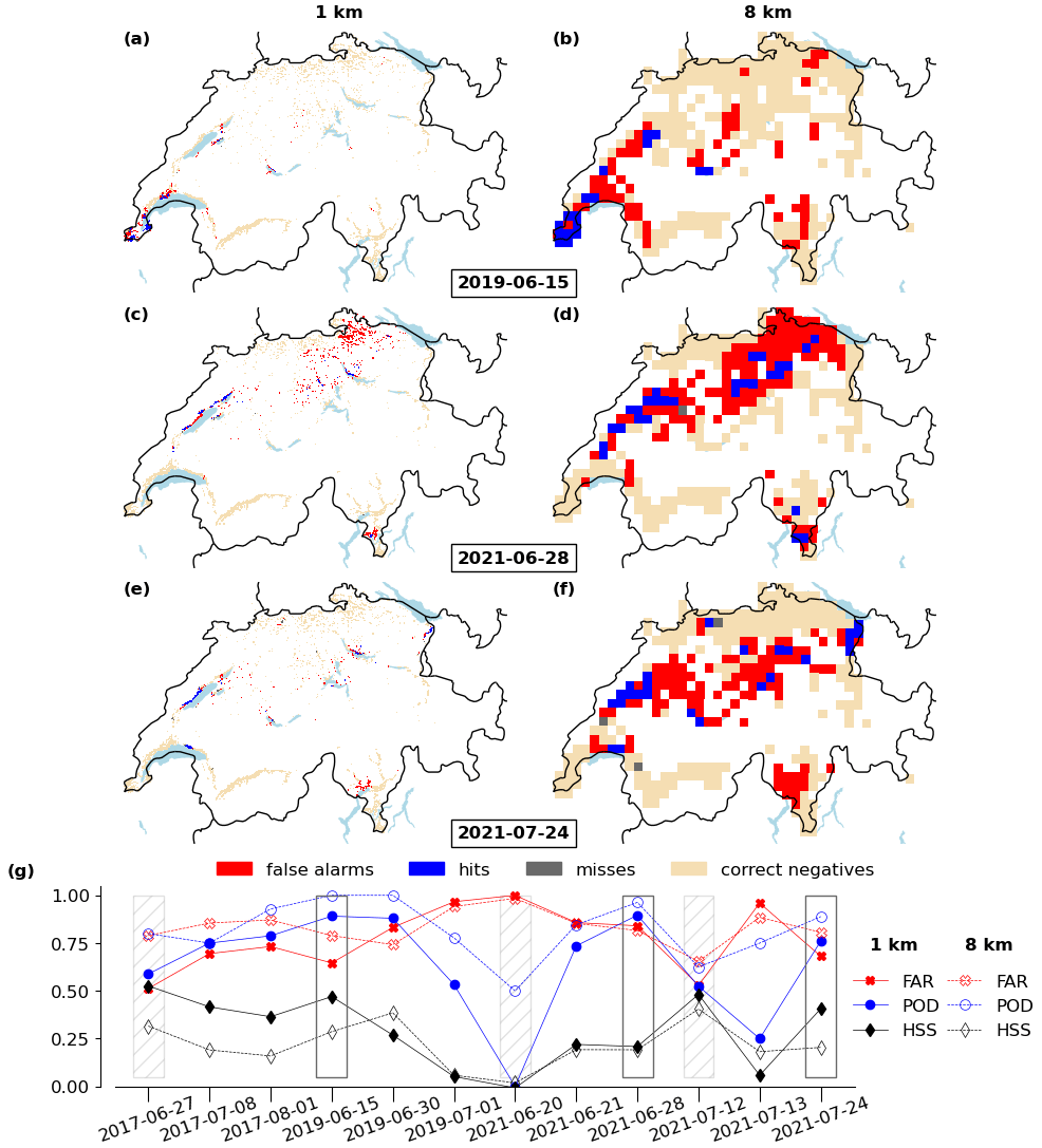
Figure 4 As Fig. 3 but for grapevine on (a, b) 15 June 2019, (c, d) 28 June 2021, and (e, f) 12 July 2021 and (g) FAR, POD, and HSS for all 12 recorded events. Grey hatched boxes in panel (g) show events with a modelled damage footprint below 80 km².

Reducing the resolution to 8 km affects the verification statistics for the three cases differently (Fig. 3b, d, f, and g). The shifted forecast (15 June 2019; Fig. 3b) greatly improves (HSS = 0.42) due to a substantially higher POD (0.93) and a lower FAR (0.67). This is mainly because the coarser resolution compensates for the spatial shift of a few kilometres, which turns misses and false alarms into hits. The over-forecast (28 June 2021; Fig. 3d) also improves (HSS = 0.38) but mostly because of a lower FAR (0.57), while POD remains unchanged. The coarser resolution effectively eliminates the red “holes” of false alarms that occur between the blue areas of hits. However, its impact on misses is limited, considering they were already minimal at the 1 km resolution. Similarly, the more cohesive damage footprint at 8 km, in comparison to 1 km, contributes to a reduced FAR (0.38) for the good forecast (12 July 2021; Fig. 3f). However, the overall skill remains largely unchanged due to the increased significance of individual scattered damage reports over the Swiss Plateau, resulting in a lower POD (0.55; without these reports, POD would be 0.73). HSS increases for all 10 considered events if spatial resolution is reduced from 1 to 8 km (Fig. 3g). However, there are substantial differences in the magnitude of the increase between events. The FAR reduces with lower resolution for all events, and POD increases for 7 out of 10 events. POD does not increase for events where it is already very high (e.g. the over-forecast) or where many misses are located far away from the modelled damage footprint (e.g. the good forecast).

For grapevine, the story is different (Fig. 4), as illustrated with the 15 June 2019 event. At 1 km, the model predicts damage footprints for grapevine well (HSS = 0.47; Fig. 4a and g). Reducing the resolution to 8 km in this case increases the FAR from 0.65 to 0.78 and reduces HSS to 0.30 despite a higher POD (Fig. 4b and g). A similar behaviour is observed for the 24 July 2021 event (Fig. 4e, f, and g), while for the 28 June 2021 event, the skill remains unchanged (Fig. 4c, d, and g). Considering all events, the following overall pattern emerges (Fig. 4g): reducing the resolution reduces HSS or does at least not increase it significantly despite a higher POD. This is in contrast to the behaviour for wheat. The difference mostly arises because FAR generally increases for grapevine but consistently decreases for wheat. A key difference between the two considered crops is that the damage footprints for grapevine are more heterogeneous and scattered than for wheat due to the very localized distribution of grapevine in the landscape compared to the spatially more even distribution of wheat. Many false alarms appear in the regions with a low density of grapevine, while hits populate the regions with high grapevine density, notably at the shores of Lake Geneva and the Three Lakes Region in western Switzerland and Lake Zurich in the north-east. Reducing the resolution mainly increases the fraction of these false alarms, leading to lower skill (Fig. 4e–g).

It is clear that the scale effect tends to reduce FAR with coarser resolution, irrespective of the crop's spatial distribution. To understand the behaviour for grapevine, an additional effect of a coarser resolution on FAR has to be considered: the chance of a false alarm also depends on cropland density (hereafter referred to as the density effect). The main reason for this is the enormous variability in hail within a storm at the scales of a few hundred metres (Morgan and Towery, 1975; Ortega et al., 2009) combined with insured fractions of fields well below 100 %. Hence, the average FAR at 1 km grid points with 1 field is higher (wheat: 82 %; grapevine: 79 %) than at grid points with 10 fields (wheat: 74 %; grapevine: 60 %). In conclusion, if cropland density strongly decreases with coarser resolution, FAR will increase accordingly. For a crop that is widespread across the domain, average cropland density within a grid cell is less dependent on the resolution (even if density within individual 1 km grid cells varies). However, the more a crop occurs fragmented in distinct parts of the domain, the stronger cropland density decreases with coarser resolution. Hence, this density effect contributes to an increase in FAR. For wheat, the average cropland density within a grid cell decreases by slightly more than a factor of 2 from 4.6 fields per square kilometre at 1 km to 1.9 fields per square kilometre at 8 km resolution. For grapevine, however, it decreases from 36.7 fields per square kilometre to 4.2 fields per square kilometre which is about a factor of 9 (note that the results are almost identical if cropland area fraction is used). The reason for these differences can also be expressed in terms of an areal inflation factor, i.e. the area covered by all exposure grid cells at a given spatial resolution divided by the area covered by all exposure grid cells at 1 km resolution. By this definition, the inflation factor is 1 at 1 km resolution and increases for coarser resolutions (Fig. A2). At all resolutions, these inflation factors are much larger for grapevine than for wheat.

In conclusion, the scale effect dominates over the density effect for wheat, and the density effect dominates over the scale effect for grapevine. Hence, to achieve a good skill when modelling hail damage footprints it is beneficial to reduce the resolution from the original 1 km to about 8 km for field crops, while 1 km provides the best skill for grapevine.

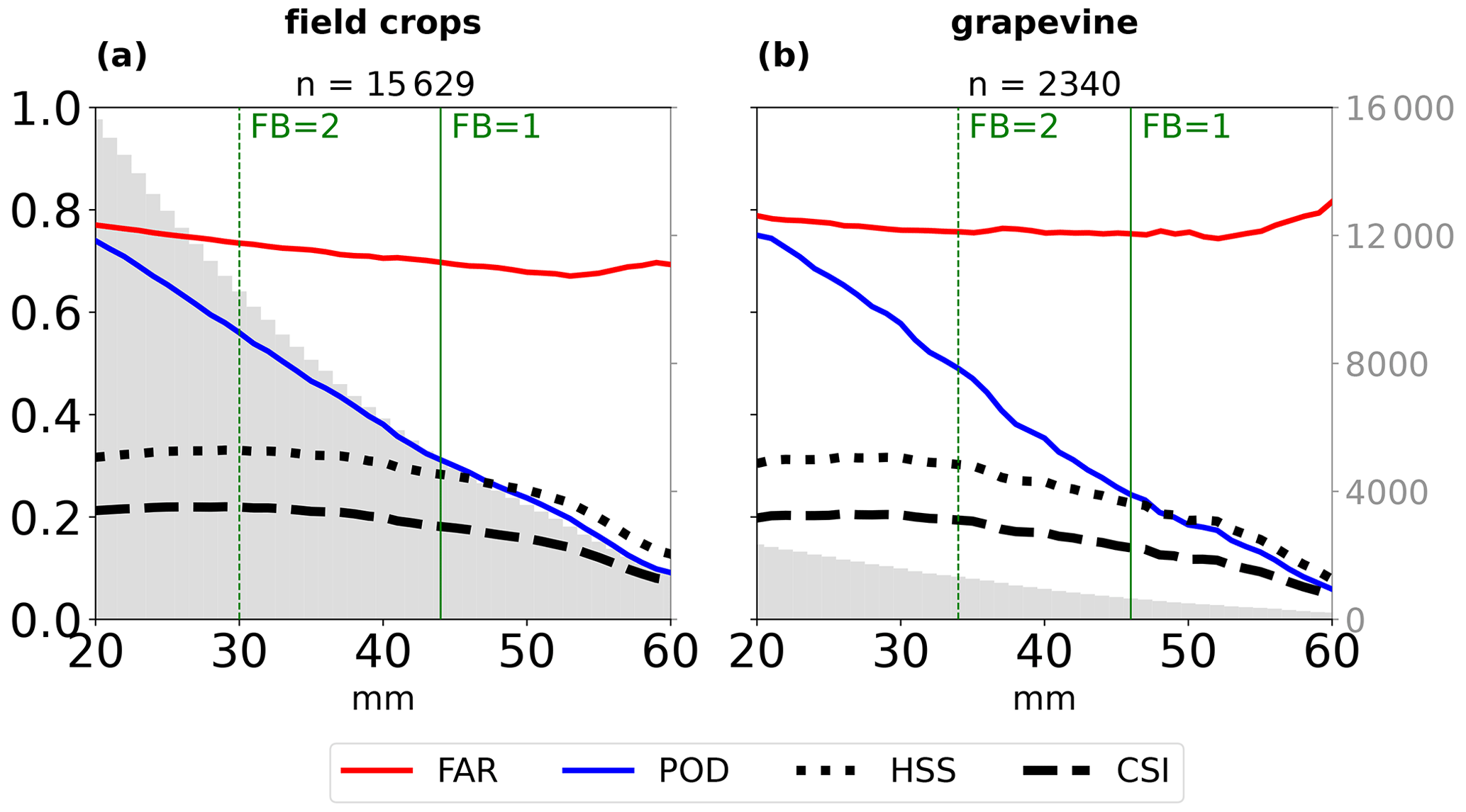
Figure 5 POD (blue), FAR (red), HSS (dotted black), and CSI (dashed black) as a function of MESHS threshold for (a) field crops and (b) grapevine at 1 km resolution. Vertical green bars show thresholds with frequency biases (FB) of approximately 1 and 2, and grey bars show the total number of hail damage predictions (hits and false alarms) at each threshold, as indicated by the vertical axis on the right. The total number of predictions for a MESHS threshold of 20 mm is indicated at the top of each panel.

3.2 The effect of MESHS threshold on model skill

Next, we aim to identify suitable MESHS threshold(s) to model hail damage footprints for field crops and grapevine. An often used method to determine an ideal hail intensity threshold is to evaluate a skill metric (e.g. HSS or CSI) as a function of threshold and determine the location of the maximum (e.g. Puskeiler et al., 2016; Kunz and Kugel, 2015). However, for wheat and grapevine at 1 km resolution, CSI and HSS do not exhibit a clear maximum. They remain largely unchanged up to 40 mm for field crops and 35 mm for grapevine and decline at higher thresholds (Fig. 5). Note that the sample size for grapevine is substantially smaller, especially at large MESHS thresholds (grey bars in Fig. 5), leading to larger uncertainty of the exact skill values. Warren et al. (2020) suggest to additionally constrain the optimal threshold with the condition that FB is close to 1 to avoid over-forecasting. Here, this would result in an optimal threshold above 40 mm for wheat and 45 mm for grapevine. Conversely, a MESHS threshold of 30 mm for field crops would result in a frequency bias of 2; i.e. it results in twice as many forecasts than observations. Hence, selecting a threshold comes with a trade-off between (i) a high POD (blue line in Fig. 5) and (ii) a low FAR (red line in Fig. 5) and FB closer to 1.

3.3 Combined effects of resolution and threshold on model skill

To provide an overview of the combined effects of resolution and threshold on model skill, the performance diagram is used (Fig. 6; Roebber, 2009; Wilks, 2019). The performance diagram shows the relationship between POD and 1-FAR (i.e., one minus the false alarm ratio, also known as the success ratio) for spatial resolutions of 1, 4, and 8 km and MESHS thresholds of 20, 30, and 40 mm. A perfect model is located in the top right of the diagram. For field crops (Fig. 6a) it becomes evident that, for all three resolutions, an increase in the threshold strongly reduces POD but also reduces FAR and FB (dashed diagonal lines), leaving its skill, as measured by CSI, practically unchanged (shading). Reducing the model resolution shifts the points in the diagram towards the top right, i.e. increases the skill by strongly decreasing FAR and increasing POD. Note that the more favourable skill measure, HSS, can not be shown in the performance diagram directly, as, unlike CSI, it also depends on the number of correct non-events, d. However, CSI behaves similar to HSS for resolutions below 8 km.

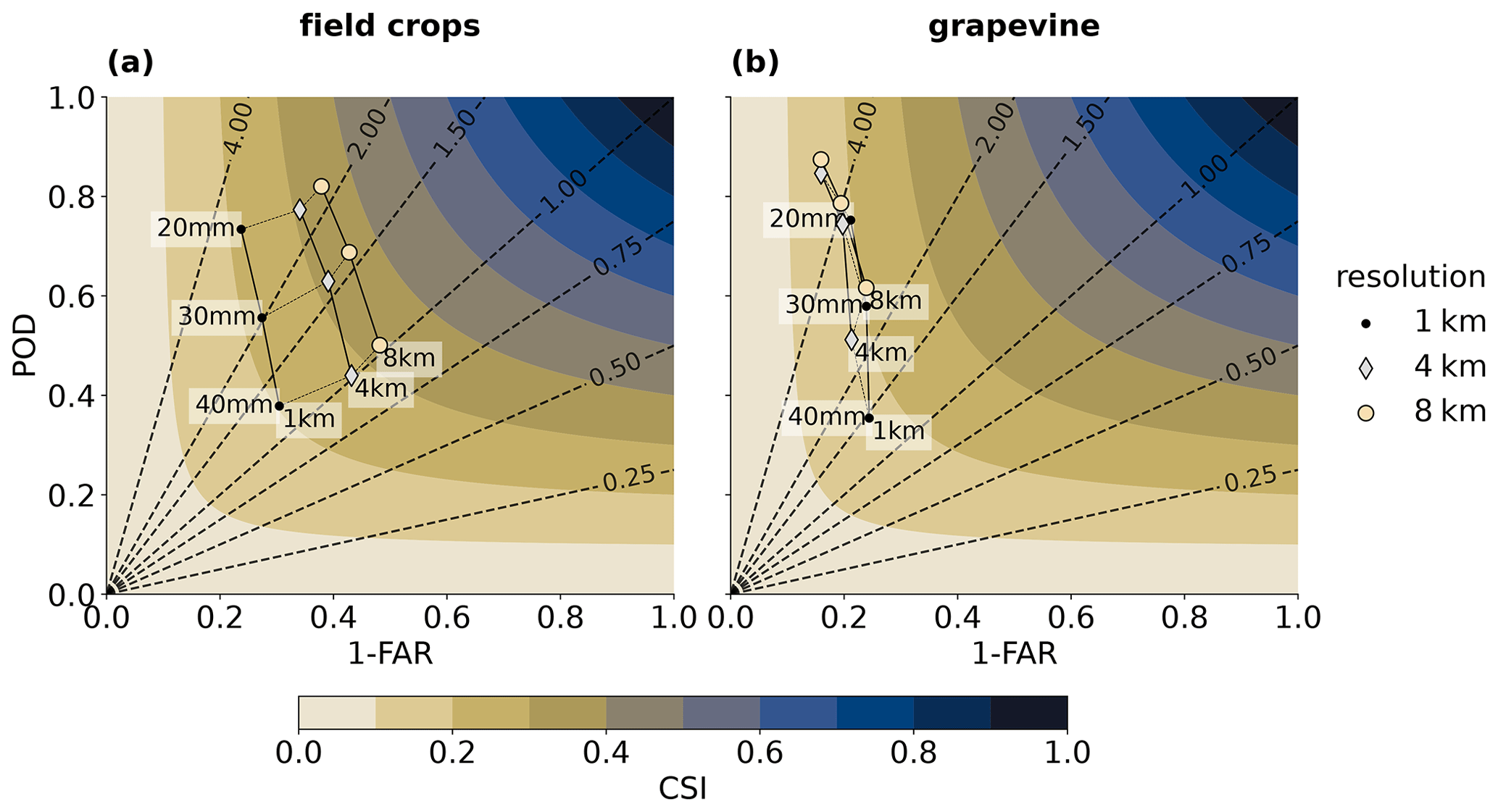
Figure 6 Performance diagrams showing POD versus 1-FAR, CSI (shading), and frequency bias (dashed lines) for (a) field crops and (b) grapevine for MESHS thresholds of 20, 30, and 40 mm and spatial resolutions of 1, 4, and 8 km.

The diagram also reveals the key differences between grapevine and field crops (Fig. 6b). Consistent with the results from Sect. 3.1, the main difference is that, for grapevine, the FAR is not reduced with coarser resolution but even slightly increased for a given threshold (i.e. the “threshold–resolution web” is squeezed together in the horizontal direction). This results in a tendency for lower skill despite the small increase in POD. An exception is the slight increase in CSI for the 40 mm threshold from 1 to 8 km resolution due to a substantial increase in POD and an almost unchanged FAR. This is because in this region of the phase space, CSI is more sensitive to changes in POD than changes in FAR.

3.4 Sensitivity to cropland density and hazard variable

Here, the sensitivities of the model performance to cropland density (via n_thresh) and the selection of an alternative radar product (POH) are discussed.

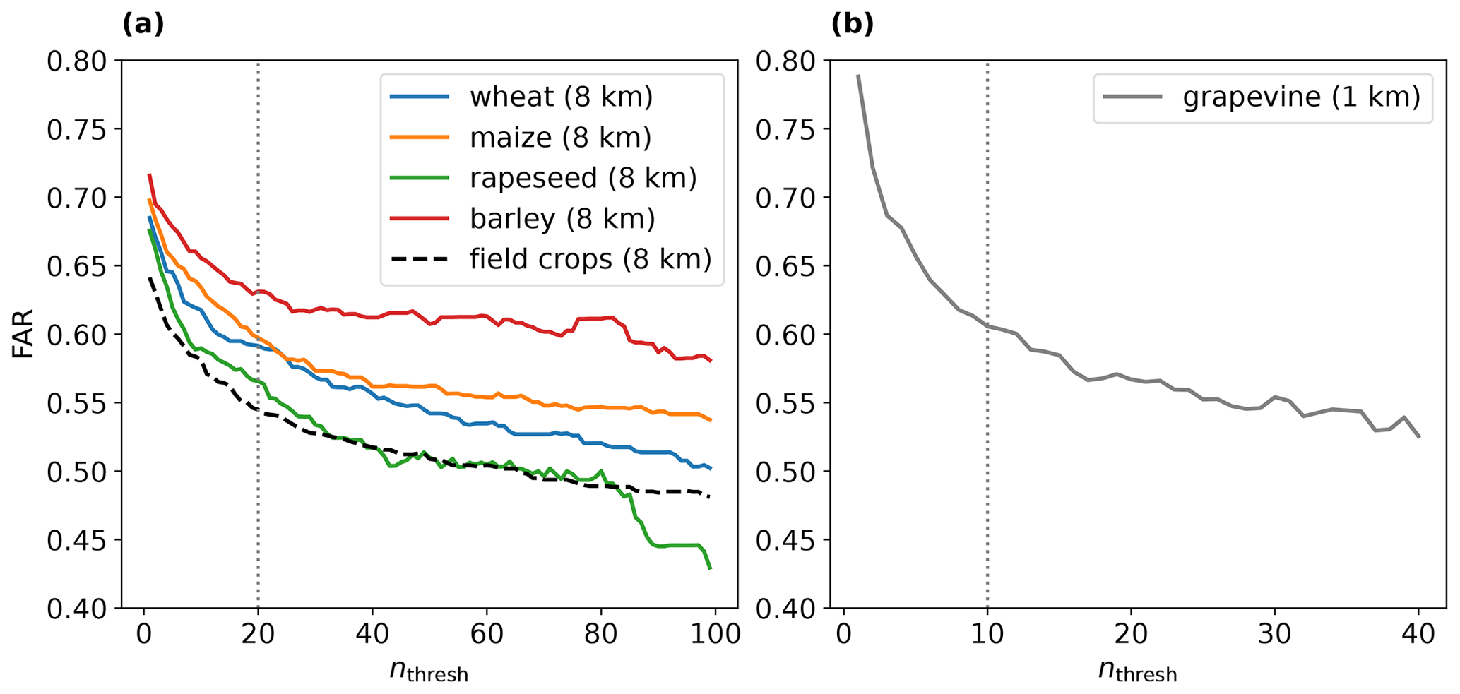
Figure 7 Change in FAR as a function of n_thresh (number of fields per grid cell) for (a) wheat (blue), maize (orange), rapeseed (green), barley (red), and field crops (black, dashed) at 8 km resolution and for (b) grapevine at 1 km resolution. The vertical bars denote pragmatic choices of n_thresh that limit FAR but still retain a large fraction (> 95 %) of the total exposed crop area and number of fields.

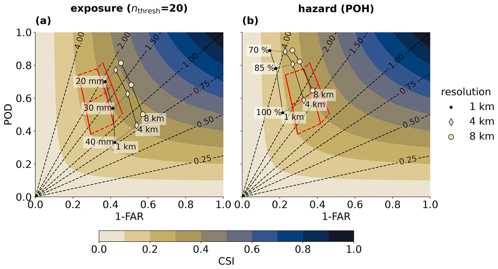
Figure 8 Performance diagrams for field crops for (a) alternative exposure with n_thresh = 20 and (b) an alternative radar product (POH at thresholds of 70 %, 85 %, and 100 %). The values indicated with the red shape correspond to those shown in Fig. 6a (MESHS, n_thresh = 1).

The sensitivity to cropland density is substantial. An increase in n_thresh leads to a decrease in FAR for all crops (Fig. 7), while POD remains largely unaffected (not shown). For n_thresh values up to around 20 for field crops (8 km resolution) and 10 for grapevine (at 1 km resolution), the FAR decreases strongly by about 10 percent points for field crops and about 20 percent points for grapevine. Beyond these thresholds, the curve tends to flatten out. Increasing n_thresh comes with the cost that the fraction of fields included is reduced (Fig. A3). Hence, an optimal value of n_thresh reduces FAR as much as possible but keeps the included fraction of fields or crop area high. Here, a pragmatic choice for all field crops at 8 km resolution is n_thresh = 20, which maintains 95 % of fields for rapeseed, 96 % for barley, 98 % for wheat and maize, and 99 % for the combined field crops (Fig. 7a). Note that, for certain crops, even higher n_thresh values are justified (e.g. wheat, maize, field crops; see Fig. A3a). For the aggregate crop class field crops, n_thresh = 100 (or larger) still preserves 96 % of fields; however, the associated reduction in FAR is rather modest (approx. 5 percentage points). Very similar numbers are the result when crop area is considered instead of field number. For grapevine at 1 km resolution, a suitable choice is n_thresh = 10, which reduces FAR by almost 0.2 and still preserves 95 % of the number of vineyards (Figs. 7b and A3b). However, it conserves only 86 % of vineyard area, which would also justify a lower threshold.

The effect of n_thresh = 20 for field crops on model performance is illustrated using a performance diagram (Fig. 8a). For all resolutions, the threshold–resolution web shifts to the right in the diagram compared to the original n_thresh = 1. Hence, FAR is substantially reduced, and POD remains nearly constant, leading to higher skill. Note, however, that the choice of the optimal n_thresh heavily depends on the chosen spatial resolution. In other words, an n_thresh = 20 preserves 99 % of field crops at 8 km resolution but less than 30 % at 1 km resolution.

Finally, the sensitivity of model performance to the selection of POH instead of MESHS is tested (Fig. 8b). The model is tested for POH thresholds of 70 %, 85 %, and 100 % at spatial resolutions of 1 4, and 8 km and with n_thresh = 1. Compared to MESHS, the threshold–resolution web is shifted towards the top left in the performance diagram. This indicates higher POD but also a higher FAR and lower overall skill. These results are consistent with previous studies (Nisi et al., 2016; Schmid et al., 2024). Further, the highest possible threshold (100 %) still exhibits a large frequency bias (> 1.5), limiting POH-based models to applications where over-forecasting is not a problem.

3.5 Discussion

The optimal resolution was found to differ for field crops (8 km) and grapevine (1 km). It was argued that two competing effects play a role: first, the scale effect tends to increase skill for coarser resolutions because larger distances between forecast and observed damage are tolerated (Warren et al., 2020; Schwartz, 2017; Schmid et al., 2024). Second, the fact that the area covered by the exposure grid cells is artificially inflated with coarser resolution leads to lower cropland densities and hence higher chances of false alarms, which reduces skill (density effect). The effect of a changing cropland density is particularly relevant because hail storms are very localized phenomena with a high within-storm spatial variability (Morgan and Towery, 1975; Ortega et al., 2009). The density effect strongly depends on the spatial distribution of crops: it is larger for crops that are scattered unevenly (like grapevine) and smaller for crops that occur more homogeneously distributed across the domain (like wheat and other field crops). Hence, reducing the spatial resolution is only beneficial for crops that are sufficiently evenly distributed in the landscape. We acknowledge that it remains open what “sufficiently” means in this context. The dependence of cropland density on spatial resolution has also been discussed by Griffith et al. (2000). In fact, it is a property that can be found for the aggregation of any spatially heterogeneously distributed feature. For example, Baker et al. (2007) found that the density of drainage channels per unit area strongly decreased with coarser resolution.

Considering the MESHS threshold, the identified trade-off between achieving either a high POD or a low FAR and an FB close to 1 signifies that the optimal threshold depends on user needs and the relative costs of a false alarm versus a missed event. For example, if an insurance company wants to use this model to verify damage claims, it will prioritize a low threshold with a high POD. On the other hand, if scientists or governments use this model to communicate the damaged crop area after a hail event, they may want to avoid a systematic overestimation of the damage extent and choose a higher threshold. To incorporate the costs of false alarms and missed events in decision-making with this model, user-tailored cost–loss models would have to be developed (de Elía, 2022). It is important to note that the best threshold for end users is not necessarily the one with the highest skill but depends on their specific cost functions (Manzato, 2007).

The strongly reduced FAR with a larger minimum number of fields within a grid cell (n_thresh) is again related to the large within-storm spatial variability in hail. The lower the cropland density, the higher the chances that a hail event does not lead to damage; i.e. a false alarm occurs despite the presence of hail. Hence, hail damage footprints can be better modelled within the main crop production areas. These results are comparable to Tian et al. (2018), who found that the FAR of satellite-based detection of rainfall decreases with increased rain gauge density.

Finally, it is noted that other verification procedures exist than the ones used in this study. Two alternatives and their effect on our results are briefly discussed. First, Ebert and Milne (2022) suggest the use of the Pierce skill score (PSS; Peirce, 1884) as an alternative to HSS for rare and severe events. One of their arguments in favour of PSS is that it is the only skill measure taking into account that, for rare and severe events, misses tend to be more problematic than false alarms. For more details on this discussion, the reader is referred to Ebert (2008). PSS favours a high POD and hence, in our case, a MESHS threshold of 20 mm. Because of its high POD, a POH-based model therefore outperforms a MESHS-based model when evaluated using PSS instead of HSS. PSS of the MESHS-based model for field crops remains nearly constant with coarser resolution until 8 km but decreases for even coarser resolutions, which corroborates the meaningfulness of the selection of an 8 km resolution.

Second, the use of fuzzy forecast verification has been proposed as an alternative to point-based techniques to verify precipitation forecasts (Ebert, 2008). An often-used fuzzy verification metric is the fraction skill score (FSS), which measures the fractional coverage of events in windows of different length scales around observations and forecasts (Roberts and Lean, 2008). It can be used to identify the scale at which a forecast should be believed. Using n_thresh = 20 we find that models for field crops are skilful (FSS ≥ 0.5) beyond a scale of 4 km and for MESHS thresholds between 20–30 mm. In general, the skill increases with larger scales and lower model resolutions. However, the 8 km model does not have a larger FSS than the 4 km model. This perspective confirms that modelling hail damage footprints is not skilful at the 1 km scale but suggests that a 4 km resolution could also be a suitable choice. Considering grapevine (n_thresh = 10), the lowest scale at which skilful prediction is possible is 6 km at a threshold of 20 mm. The FSS confirms that the skill does not improve with coarser spatial resolution except for very large scales beyond 64 km.

Table 3 Most suitable model setups (resolution, MESHS threshold s, cropland number density threshold n_thresh) for field crops (aggregate crop class including wheat, maize, rapeseed, and barley) and grapevine with the associated skill metrics, including the probability of detection (POD), the false alarm ratio (FAR), the Heidke skill score (HSS), and the frequency bias (FB).

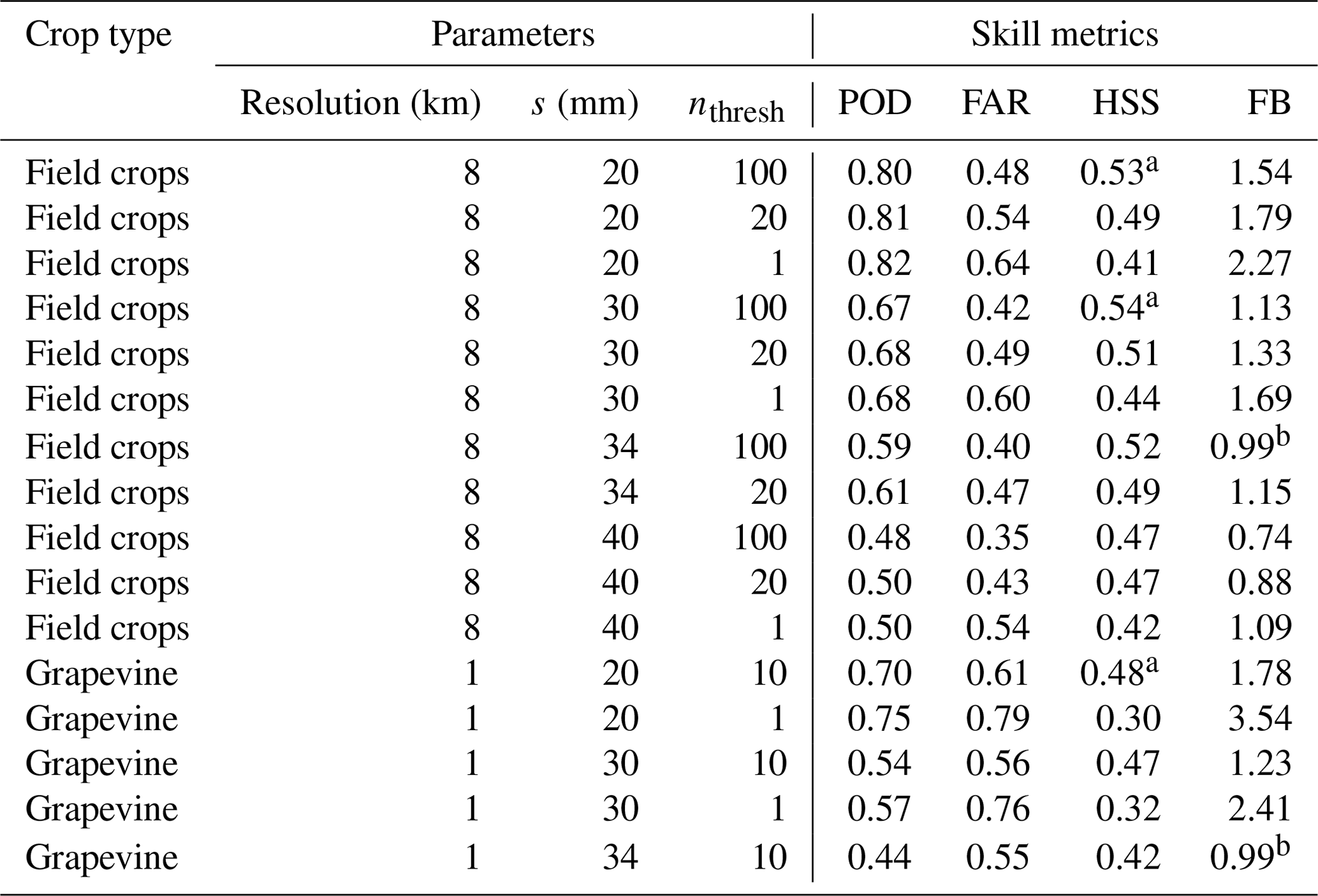
^a Highest skill for this crop type. ^b Frequency bias closest to 1 for this crop type. Note that n_thresh = 100 is only a sensible choice for the aggregate field crops class due to its high cropland density. For individual crop types, lower values like n_thresh = 20 are to be preferred.

4 Conclusions

This study presents an open-source model implemented in the open-source natural catastrophe modelling platform CLIMADA (Aznar-Siguan and Bresch, 2019) to predict hail damage footprints (occurrence of hail damage) for individual crops after the passage of a hailstorm based on the operational single-polarization meteorological radar product MESHS and detailed agricultural land use data. Damage information from a crop insurer was used to quantify the skill of the model with different skill metrics. The main goal was to assess the model performance for different choices of spatial resolution (aggregation), MESHS threshold, and threshold of the minimum number of fields used to define exposure (cropland density).

For field crops (wheat, maize, rapeseed, barley) the model performance improves substantially when coarsening spatial resolution from 1 to 8 km, mainly because it relaxes the requirement for exact spatial overlap of modelled and observed damage footprints (scale effect). Beyond 8 km, model skill tends to reduce again. In contrast, for grapevine, coarser resolution tends to lower model skill. We conclude that this difference between field crops and grapevine is mainly related to the different spatial distribution of these crops in the landscape (scattered for grapevine versus more homogeneous for field crops), which determines how strongly cropland density decreases with coarser resolution. A lower cropland density leads to a higher chance of a false alarm (density effect). For wheat, the scale effect dominates, while for grapevine the density effect dominates.

Increasing the MESHS threshold from 20 to 40 mm strongly decreases the probability of detection (POD) for hail damage but also reduces false alarm ratio (FAR) and frequency bias (FB). The overall skill (HSS) is only moderately affected by the threshold selection due to the trade-off between POD and FAR that has to be aligned with user needs and their specific cost functions.

Model performance can be substantially improved at all resolutions by selecting a higher minimum cropland density (n_thresh) for the exposure definition mainly due to a reduction in FAR. Considering an alternative radar-based hail product (POH) reveals higher POD, higher FAR, and lower skill compared to MESHS, confirming previous studies (Nisi et al., 2016; Schmid et al., 2024).

Finally, the key skill metrics of selected representative model setups for the best resolution (8 km for field crops, 1 km for grapevine) are shown in Table 3. For all crops, MESHS thresholds of 20 and 30 mm outperform a MESHS threshold of 40 mm, in particular for higher n_thresh. In general, a larger n_thresh will yield results closer to the “true” skill of MESHS, i.e. the skill it would have given a gapless hail detection network on the ground, but comes at the cost of a reduced number of data points for verification. The best-performing setups (HSS∼0.53) for field crops are achieved at 8 km resolution and reach a POD of about 0.8 combined with a FAR of about 0.5 (for MESHS > 20 mm) or a POD around 0.7 combined with a FAR of about 0.4 (for MESHS > 30 mm). For grapevine, the best performance (HSS ∼ 0.48) is achieved at 1 km and reaches either a POD of around 0.7 and a FAR of 0.6 (for MESHS > 20 mm) or a POD and FAR of around 0.55 (for MESHS > 30 mm). We note again that the suitable threshold depends on the purpose for which the model is used. For climatological purposes, it is important that the frequency bias is close to 1. While thresholds of 20–30 mm strongly overpredict damage occurrence (FB > 1), a threshold of 40 mm underpredicts it (FB < 1). The MESHS threshold with FB closest to 1 is 34 mm for both field crops at 8 km and grapevine at 1 km and is hence recommended to derive accurate climatological frequencies of crop hail damage occurrence.

These results are comparable to previous verification efforts of MESHS (Nisi et al., 2016) or the original Waldvogel et al. (1979) criterion (Puskeiler et al., 2016), as well as MESH (Cintineo et al., 2012; Skripniková and Řezáčová, 2014; Kunz and Kugel, 2015; Warren et al., 2020), although methodological verification approaches substantially differ from ours. Traditionally, verification of radar-based hail detection has focused on the dependence of the skill on the hail intensity threshold. Our work highlights that it is crucial to also consider the dependence on spatial scale and the density of the verification data.

The model presented here provides a first step towards the (operational) modelling of hail damage as well as hail risk assessments for crops in Switzerland. It is important to note that larger damage datasets would substantially increase the robustness of the results due to the large event-to-event variability. Gridded exposure and damage information is provided open-source via the CLIMADA data API to facilitate its use for operational purposes as well as the further development and validation of (hail) damage models for crops in Switzerland.

Appendix A

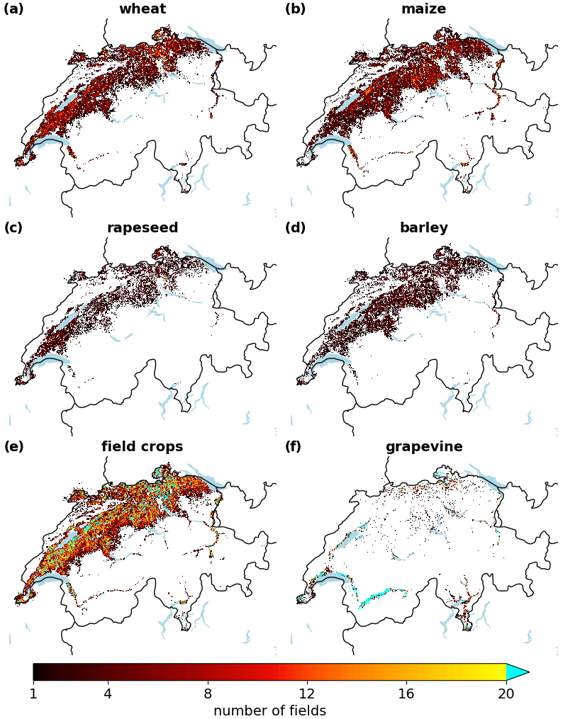
Figure A1 Cropland number density at 1 km spatial resolution for (a) wheat, (b) maize, (c) rapeseed, (d) barley, (e) field crops, and (f) grapevine.

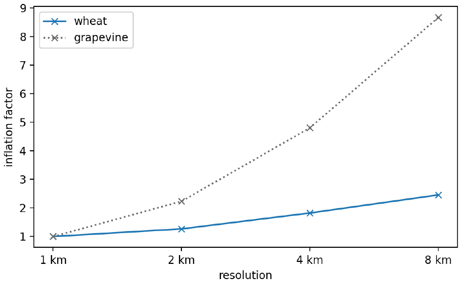
Figure A2 Total area covered by all exposure grid cells at a given spatial resolution divided by the area covered by all exposure grid cells at 1 km resolution (inflation factor) for wheat (blue) and grapevine (grey, dashed).

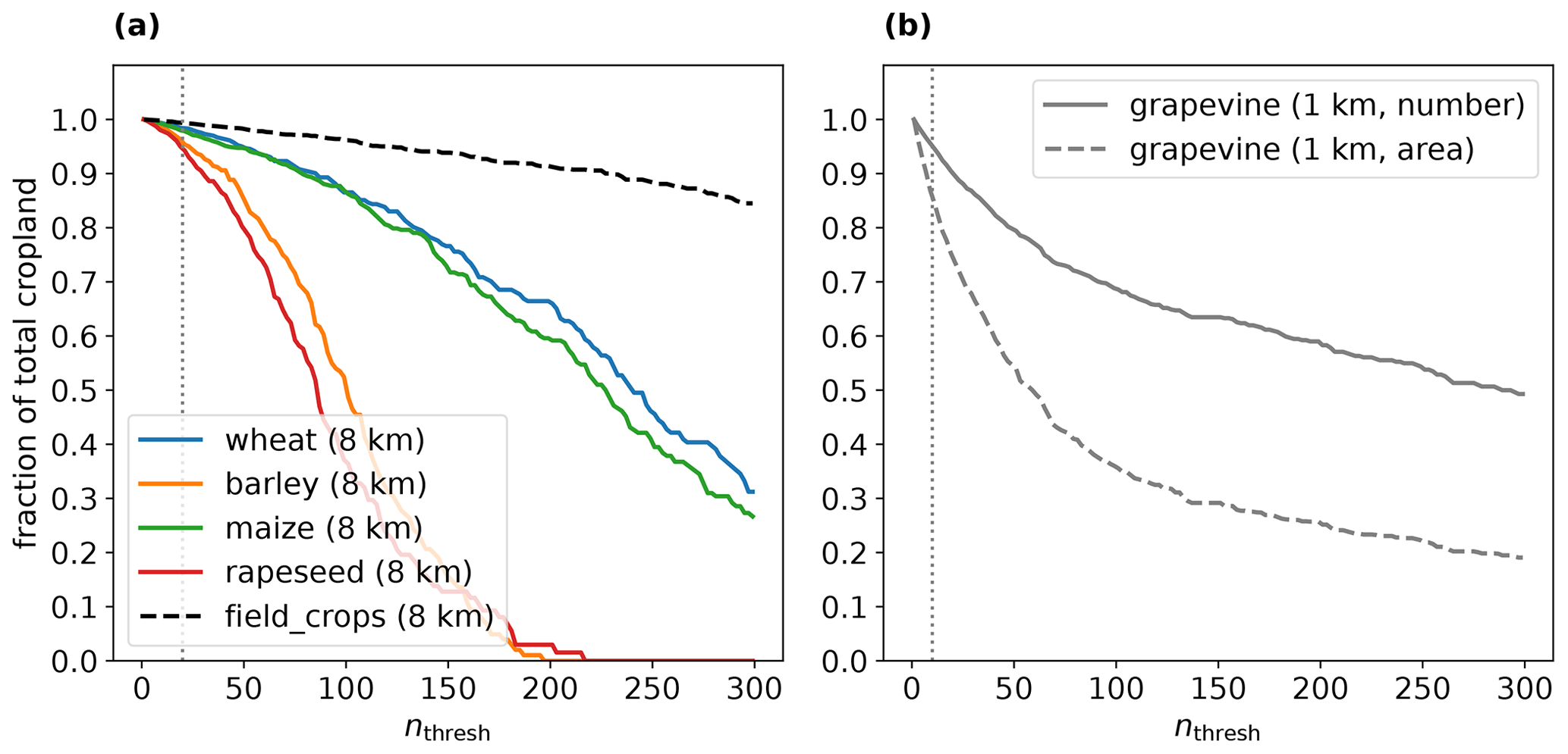
Figure A3 Change in the fraction of total number of fields included in the exposure as a function of n_thresh for (a) wheat (blue), maize (orange), rapeseed (green), barley (red), and field crops (black, dashed) at 8 km resolution and for (b) grapevine at 1 km resolution. In (b) the fraction of cropland area is also shown (dashed) because it deviates substantially from the fraction of fields for grapevine but not crops shown in panel (a). The vertical bars denote the pragmatic choices of n_thresh (panel a: 20; panel b: 10) that avoids FAR that is too high but still includes a large fraction (> 95 %) of total exposed crop area and number of fields (see Fig. 7).