Nonlinear processes in tsunami simulations for the Peruvian coast with focus on Lima and Callao

This investigation addresses the tsunami inundation in Lima and Callao caused by the massive 1746 earthquake (M_w 9.0) along the Peruvian coast. Numerical modeling of the tsunami inundation processes in the nearshore includes strong nonlinear numerical terms. In a comparative analysis of the calculation of the tsunami wave effect, two numerical codes are used, Tsunami-HySEA and TsunAWI, which both solve the shallow water (SW) equations but with different spatial approximations. The comparison primarily evaluates the flow velocity fields in inundated areas. The relative importance of the various parts of the SW equations is determined, focusing on the nonlinear terms. Particular attention is paid to the contribution of momentum advection, bottom friction, and volume conservation. The influence of the nonlinearity on the degree and volume of inundation, flow velocity, and small-scale fluctuations is determined. The sensitivity of the solution concerning the bottom friction parameter is also investigated, showing the effects of nonlinearity processes in the inundated areas, wave heights, current velocity, and the spatial structure variations shown in tsunami inundation maps.

1 Introduction

Over the past couple of decades, after the catastrophic 2004 M_w 9.3 Sumatra earthquake and widespread tsunami (Titov et al., 2005a; Kowalik et al., 2005; Grilli et al., 2007; Syamsidik et al., 2021), there has been an increased need for a more detailed study of these natural hazards. The understanding of such hazards has greatly improved due to the development of numerical models and methods that can reproduce various hazard and risk scenarios, as well as use them for community preparedness and mitigation (Berke and Smith, 2009; Shmueli et al., 2021). Mega-tsunamis, such as those that struck the Indian Ocean in 2004 and after the Tohoku earthquake in 2011, are notable for their impacts at local scales and can affect regions across large geographic distances. Both of these massive tsunamis were recorded as far as the South American coasts (Rabinovich et al., 2017). As the tsunami flowed, waves suffered reflection from continents and from the abrupt changes in the bathymetry and coastal topography (Arcas and Titov, 2006; Rabinovich et al., 2017), and were affected by various atmospheric processes (Broutman et al., 2014), all of which significantly distorted the original signal. As the tsunami waves approached the coast, they were modified considerably by the continental shelf and local topography. In addition to the factors influencing the propagation of a tsunami wave as described above, it was noted that tsunami resonance and associated fluctuations in shelf and bay modes could play a crucial role in amplifying tsunami waves (Aranguiz et al., 2019). All these processes are highly nonlinear and can significantly depend on the quality of bathymetry and topography data, particularly in the nearshore (Sepúlveda et al., 2020).

The tuning required to reduce numerical uncertainties beyond those already inherent in natural phenomena can be resolved by comparing the effects of different numerical schemes. According to their purpose, tsunami models can be conditionally divided into two types. The first type includes operational models (Titov et al., 2005b), whose main task is to estimate the time of arrival of a tsunami wave and its height on a timescale faster than wave propagation in real time. Often, such models are linearized and do not perform calculations in the inundation zone. The tsunami wave height metric can be obtained using the “amplification factor”, which describes the relationship between the wave height in the open sea and the maximum inundation height for waves with different wave characteristics (Glimsdal et al., 2019). Another approach to assessing the tsunami threat can be considered based on Green's summation, using the parameters of the seismic source (Miranda et al., 2014) as input. Green's functions are calculated using a numerical SW model for linearized equations at points of the most significant interest.

Numerical models of the second kind should describe the inundation area with a very high spatial resolution and have reliable numerical wetting/drying schemes, which are associated with relatively high energy consumption in the computational aspect. In addition, often, the time between the occurrence of a tsunami and its approach to the coast is minimal, and then pre-calculated databases of possible scenarios of tsunami sources and numerical modeling (Macías et al., 2017; Rakowsky et al., 2013) come to the rescue. The advantage of such models compared with operational ones is a more accurate and detailed description of the processes occurring in the inundation area (Baba et al., 2014; Harig et al., 2022). The choice of operational information is no longer based on calculations during the event and analysis of inundation areas according to some assumptions but on the appropriate scenario, which can be refined when correcting the source of tsunami wave formation (Harig et al., 2020).

Numerical models for calculating surface gravity waves, including tsunami waves, within the framework of SW theory, depending on various approximations, can be divided into linear, nonlinear, and nonlinear dispersive. In operative models, linear equations are often used to reduce computational costs (Babeyko et al., 2010). Another advantage of such models is associated with a significantly higher time step of integrating the problem since there is no limitation on the advective mode (Androsov et al., 2002).

The shallow water equations contain three types of nonlinearity: momentum advection, nonlinearity in the continuity equation due to variable water thickness, and nonlinear friction (Androsov et al., 2011; Macías et al., 2017). All these types of nonlinearity play different roles in wave propagation near and on the coast. As shown in Androsov et al. (2013), on a steep bottom slope, when a wave approaches the shore, momentum advection plays a significant role; in extended shelf zones – nonlinearity in the continuity equation, and directly near and along the coastline – bottom friction terms (Ribal, 2008).

Several works analyze nonlinearity in tsunami models, mainly focusing on comparing the wave amplitude in linear and nonlinear problems in general. Some works link analytical solutions with practical calculations (Zahibo et al., 2006) and others compare solutions for linear problems with nonlinear systems for some areas of the world's oceans affected by tsunami waves (Pujiraharjo and Hosoyamada, 2009; Liu et al., 2009; Saito et al., 2014). In this case, the effect of different types of nonlinearity is not singled out. At the same time, the analysis of each of the components of the nonlinearity is highly dependent on the details of the local conditions, determines the importance of the relevant factors for each component of the nonlinearity, and can help in choosing the appropriate model in a given situation.

The theory of the run-up of long waves onto the shore is of considerable interest. This problem of various long symmetrical or asymmetrical waves with the same steepness of the front and rear slopes of unbroken waves onto a flat slope is quite well developed from a mathematical point of view within the framework of the nonlinear theory of shallow water, allowing for an analytical solution (Shuto, 1967; Tuck and Hwang, 1972; Pelinovsky and Mazova, 1992; Massel and Pelinovsky, 2001; Tinti and Tonini, 2005). As a result, formulas for run-up height can be parameterized to include the height and length of the suitable wave and the distance to shore; such numerical results agree with laboratory experiments. At the same time, according to numerous observations of the 2004 tsunami, due to the transformation of the wave when moving along heterogeneous bathymetry, a strongly deformed wave with a noticeable steepness of the front slope approaches the shore. Didenkulova et al. (2006) showed that a wave with an increased steepness of the front slope penetrates further onto the coast than a wave with a symmetrical profile.

The nonlinear-dispersion terms qualitatively and quantitatively change the amplitude and shape of the wave as it passes over an underwater obstacle or wave run-up on a vertical barrier (Beji and Battjes, 1993; Viotti et al., 2014) and with an increase in the steepness of the tsunami wave front (Tsuji et al., 1991; Elsheikh et al., 2022). Accounting for dispersion in the model is associated with significant numerical limitations (ultra-high grid resolution and small integration step) and is mainly used in comparative analysis (Horrillo et al., 2006; Pujiraharjo and Hosoyamada, 2009). Horrillo et al. (2006) noted that including dispersion in numerical models is necessary for a more accurate description of the interaction of a tsunami wave with partial reflection from the continental shelf and when entering sea bays where resonant oscillations can occur. However, there need to be more coastal observations to support this. As for the passage of a tsunami wave in the deep ocean, a comparative analysis shows that the nonlinear shallow water models are quite reliable for practical purposes and show a high degree of agreement with observations, and the inclusion of dispersion only marginally improves the result (Pujiraharjo and Hosoyamada, 2009). In this regard, we do not consider the dispersion terms in our study.

This work has a twofold purpose. The first goal relates to a comparative analysis of two numerical tsunami models, TsunAWI and Tsunami-HySEA, using the example of an inundation assessment caused by a strong destructive earthquake (M_w 9.0) that occurred on 28 October 1746 and resulted in a wave of about 24 m in the city of Callao (Jimenez et al., 2013). Given that the wave run-up and tsunami inundation evolution are highly nonlinear processes, the second goal of the article is to analyze the role of each term of the nonlinearity in the numerical solution. A comparative analysis of the space–time dynamics and energy characteristics of various implementations of the TsunAWI model with combinations of included nonlinear terms in the equations is carried out.

This study provides special focus on the analysis of the variability in the solution depending on the sensitivity to the Manning coefficient in the bottom friction term. When solving a system of SW equations, depending on the choice of bottom friction coefficient (Manning parameter), there is significant uncertainty in the solution's response to a given input parameter of the model (Sogut and Yalciner, 2018). All of this points to the fact that it is almost impossible to represent the modeling of tsunami waves using a deterministic approach. Modeling the passage of tsunami waves and especially the flooding of coastal regions can be classified as the so-called stochastic model.

The article briefly describes two tsunami models, TsunAWI and Tsunami-HySEA, based on nonlinear SW equations. A distinctive feature of implementing these two models is their spatial discretization. TsunAWI operates on unstructured meshes and solves the equations with the finite element method, while the Tsunami-HySEA uses structured nested meshes and employs the finite volume method. The next section of the work is devoted to setting up the problem for these two models. Section 3 describes the simulation domain, initial conditions, and mesh characteristics. The calculation and comparative analysis of the simulation results of the two models are given in Sect. 4. In Sect. 5, based on the calculations of the TsunAWI model, an analysis of the nonlinearity contained in the equations is performed. Section 6 discusses the results of this work and concludes the study. The Appendix provides extended comparison results of the two models.

2 Description of the models

The shallow water equations (Hirsch, 1974) derived from vertically integrating the Reynolds-averaged Navier–Stokes equations under the hydrostatic assumption and Boussinesq approximation in the Ω plane domain bounded by boundary ∂Ω are considered with the general formulation as follows:

$$\begin{array}{}\text{(1)}& {\displaystyle }\begin{array}{rl}{\partial }_t\mathit{u}& +(\mathit{u}\cdot \mathrm{\nabla })\mathit{u}+f\mathit{k}\times \mathit{u}+g\mathrm{\nabla }\mathit{\zeta }-\mathrm{\nabla }\cdot A_h\mathrm{\nabla }\mathit{u}\\ & +{\displaystyle \frac{g{n}^{\mathrm{2}}\mathit{u}\left|\mathit{u}\right|}{H^{\mathrm{4}/\mathrm{3}}}}=\mathrm{0}\end{array}\text{(2)}& {\displaystyle }{\partial }_t\mathit{\zeta }+\mathrm{\nabla }\cdot \left(\mathit{u}H\right)=\mathrm{0}.\end{array}$$

For the horizontal velocity vector $\mathit{u}=(u,v)$ and the total water depth $H=h+\mathit{\zeta }>\mathrm{0}$, h is the unperturbed water depth and ζ the surface elevation, $\mathrm{\nabla }=(\partial /\partial x,\partial /\partial y)$ is the gradient operator, f the Coriolis parameter, k the unit vector in the vertical direction, g the gravitational acceleration, and A_h the eddy viscosity coefficient. Estimating the bottom friction terms involves an empirical friction Manning–Strickler parameter n, which depends on the bottom type and generally varies from 0 (frictionless bottoms) to 0.06, with typical values in the range of 0.02–0.03 (Harig et al., 2008).

On the solid part of the boundary, ∂Ω₁, and on its open part, ∂Ω₂, we impose the following boundary conditions:

$$\begin{array}{}\text{(3)}& {\mathit{u}}_n{|}_{\partial {\mathrm{\Omega }}_{\mathrm{1}}}=\mathrm{0},\mathbf{\Gamma }(\mathit{u},\mathit{\zeta }){|}_{\partial {\mathrm{\Omega }}_{\mathrm{2}}}=\mathit{F},\end{array}$$

where u_n is the velocity normal to the solid boundary, Γ is the operator of the boundary conditions, and F is the known vector function determined by the boundary regime (Oliger and Sundström, 1978; Androsov et al., 1995) and different for inflow and outflow. In tsunami models, the most common boundary information is the radiation boundary condition: ${\mathit{u}}_n=\sqrt{g{H}^{-\mathrm{1}}}\mathit{\zeta }$.

The problem (Eqs. 1–3) for $\mathit{v}=(\mathit{u},\mathit{\zeta })$ is solved for the given initial conditions:

$$\begin{array}{}\text{(4)}& \mathit{v}{|}_{t=\mathrm{0}}={\mathit{v}}^{\mathrm{0}}.\end{array}$$

The equation for the energy of the external motion mode, whose equations are vertically averaged equations, is obtained by multiplying the first of Eq. (1) by ρ₀Hu, the second by ρ₀Hv, and Eq. (2) by ${\mathit{\rho }}_{\mathrm{0}}(g\mathit{\zeta }+\frac{\mathrm{1}}{\mathrm{2}}|\mathit{u}{|}^{\mathrm{2}})$. The total energy of the mean motion, in this case, will be determined by the formula

$$\begin{array}{}\text{(5)}& E={\displaystyle \frac{\mathrm{1}}{\mathrm{2}}}{\mathit{\rho }}_{\mathrm{0}}\left(H|\mathit{u}{|}^{\mathrm{2}}+g{\mathit{\zeta }}^{\mathrm{2}}\right),\end{array}$$

which is the total energy per unit area, where ρ₀ is the average density of the seawater. The first term on the right side is kinetic energy and the second is the potential energy of the flow.

2.1 TsunAWI model

The TsunAWI model is based on finite element methods. The main reason for choosing such a method is the computational grid, which can be adapted to cover basins with uneven bottom topography and coastline without generating nested meshes. The finite element spatial discretization in the TsunAWI model is based on the approach by Hanert et al. (2005) with some modifications like added viscous and bottom friction terms, corrected momentum advection terms, radiation boundary condition, and nodal lumping of a mass matrix in the continuity equation. The basic principles of discretization follow Hanert et al. (2005) with linear conforming elements P₁ for sea surface height ζ and water depth h, as well as linear nonconforming elements $P_{\mathrm{1}}^{\mathrm{NC}}$ for the velocity u. The basic principles of the finite element discretization follow the paper of Hanert et al. (2005), and they are not repeated here.

Simulation of tsunami wave propagation benefits from using an explicit time discretization. Numerical accuracy requires relatively small time steps, reducing implicit schemes' main advantage. Furthermore, modeling the inundation processes usually requires very high spatial resolution (up to meters) in coastal regions and, consequently, many nodes, drastically increasing the necessary computational resources in cases of implicit temporal discretization. The leap-frog scheme was chosen as a simple and easy-to-implement method. We rewrite Eqs. (1) and (2) in time-discrete form:

$$\begin{array}{}\text{(6)}& {\displaystyle }\begin{array}{rl}{\displaystyle \frac{{\mathit{u}}^{k+\mathrm{1}}-{\stackrel{\mathrm{‾}}{\mathit{u}}}^{k-{\mathrm{1}}^{*}}}{\mathrm{2}\mathrm{\Delta }t}}& +\left({\mathit{u}}^k\cdot \mathrm{\nabla }\right){\mathit{u}}^k+f\mathit{k}\times {\mathit{u}}^k+g\mathrm{\nabla }{\mathit{\zeta }}^k\\ & -\mathrm{\nabla }\cdot A_h\mathrm{\nabla }{\mathit{u}}^k+{\displaystyle \frac{g{n}^{\mathrm{2}}{\mathit{u}}^{k+\mathrm{1}}\left|{\mathit{u}}^k\right|}{H^{\mathrm{4}/\mathrm{3}}}}=\mathrm{0},\end{array}\text{(7)}& {\displaystyle }{\displaystyle \frac{{\mathit{\zeta }}^{k+\mathrm{1}}-{\stackrel{\mathrm{‾}}{\mathit{\zeta }}}^{k-{\mathrm{1}}^{*}}}{\mathrm{2}\mathrm{\Delta }t}}+\mathrm{\nabla }\cdot \left(H^k{\mathit{u}}^k\right)=\mathrm{0}.\end{array}$$

Here Δt is the time step length and k is the time index. The leap-frog three-time-level scheme provides second-order accuracy and is neutral within the stability range. This scheme, however, has a numerical mode removed by the Robert–Asselin time filter procedure, ${\stackrel{\mathrm{‾}}{\mathit{v}}}^{k^{*}}={\mathit{v}}^k+\mathit{\alpha }({\mathit{v}}^{k+\mathrm{1}}-\mathrm{2}{\mathit{v}}^k+{\stackrel{\mathrm{‾}}{\mathit{v}}}^{k-{\mathrm{1}}^{*}})$, where asterisks denote filtered characteristics and α=0.01 (Asselin, 1972).

Advection is one of the essential complexities in calculating the waves of a tsunami in a shallow zone. Advection of momentum in the original formulation by Hanert et al. (2005) is very unstable. For this reason, we applied a new approach to calculate advection. This approach has appeared robust in areas of complex morphometry where advection becomes significant. To calculate the advection term in the momentum equation, we first project the velocity from the $P_{\mathrm{1}}^{\mathrm{NC}}$ to the P₁ space to smooth it. Then, we use it in the advection term and proceed by multiplying this form with a $P_{\mathrm{1}}^{\mathrm{NC}}$ basis function and integrating it over the domain. In contrast to the advection scheme proposed by Hanert et al. (2005), it has the advantage that no boundary integral has to be computed and is more stable.

For modeling wetting and drying, we use a moving boundary technique which utilizes extrapolation through the wet–dry boundary and into the dry region (Lynett et al., 2002). This concept excludes dry nodes from the solution and then extrapolates the elevation and barotropic gradient to the dry nodes from their wet neighbors.

Because the leap-frog scheme is neutrally stable, it demands horizontal viscosity in places of large gradients. The horizontal viscosity coefficient is determined by a Smagorinsky parameterization (Smagorinsky, 1963) with adding some small background coefficient.

A detailed description of the TsunAWI model and its numerical implementation is given in Androsov et al. (2011).

2.2 Tsunami-HySEA model

Tsunami-HySEA solves the two-dimensional shallow water system using a high-order finite volume method. These methods are mass preserving for arbitrary (nested) bathymetries. Tsunami-HySEA implements several reconstruction operators:

• Monotonic Upstream-centered Scheme for Conservation Laws (MUSCL; see van Leer, 1979), which achieves second order;

• the hyperbolic Marquina's reconstruction (see Marquina, 1994), which achieves third order;

• the total variation diminishing (TVD) combination of piecewise parabolic and linear 2D reconstructions, which also achieves third order.

For large computational domains and in the framework of the Tsunami Early Warning System (TEWS), Tsunami-HySEA also implements a two-step scheme similar to leap-frog for the deep water propagation step and a second-order TVD-WAF (weighted average flux) flux-limiter scheme for the close-to-coast propagation to inundation step. Combining both schemes guarantees mass conservation in the complete domain and prevents the generation of spurious high-frequency oscillations near discontinuities generated by leap-frog-type schemes. At the same time, this numerical scheme reduces computational times compared with other numerical schemes while the amplitude of the first tsunami wave is preserved. Concerning the inundation modeling, the wet- and dry-front discretization consists of locally replacing the 1D Riemann solver used during the propagation step with another 1D Riemann solver, considering the presence of a dry cell. This reconstruction step is also modified to preserve the water depth's positivity.

3 Models' setup

3.1 Domain

The Lima/Callao region is located on the central coast of Peru, characterized by a narrow strip of land between the Pacific Ocean and the Andes. The coastal zone is relatively flat, with sandy beaches and rocky cliffs interspersed along the coastline.

The bathymetry of the area is diverse: shallow water near the coast gradually deepens with distance from the coast. The continental shelf is relatively narrow and the water depth beyond it increases rapidly. The maximum depth in this area is about 2 km, located several hundred kilometers from the coast.

3.2 Bathymetry and topography data

The bottom relief is crucial for numerical simulations of wave propagation and inundation. In the deep ocean, we use the General Bathymetric Chart of the Ocean (GEBCO) dataset at a resolution of up to 15 arcsec. Particularly, the company EOMAP produced high resolution bathymetric and topographic datasets for the nearshore range based on different sources. For the water area down to about 300 m depth, a combination of nautical charts and GEBCO was incorporated. Tandem-X topography data (Krieger et al., 2007) were used for the land area. Several minor errors and inaccuracies were removed and partially interpolated from the Tandem-X data. The final output that results from merging bathymetric and topographic datasets was derived in 12 m resolution as shown in Fig. 1. More information is contained in Harig et al. (2024).

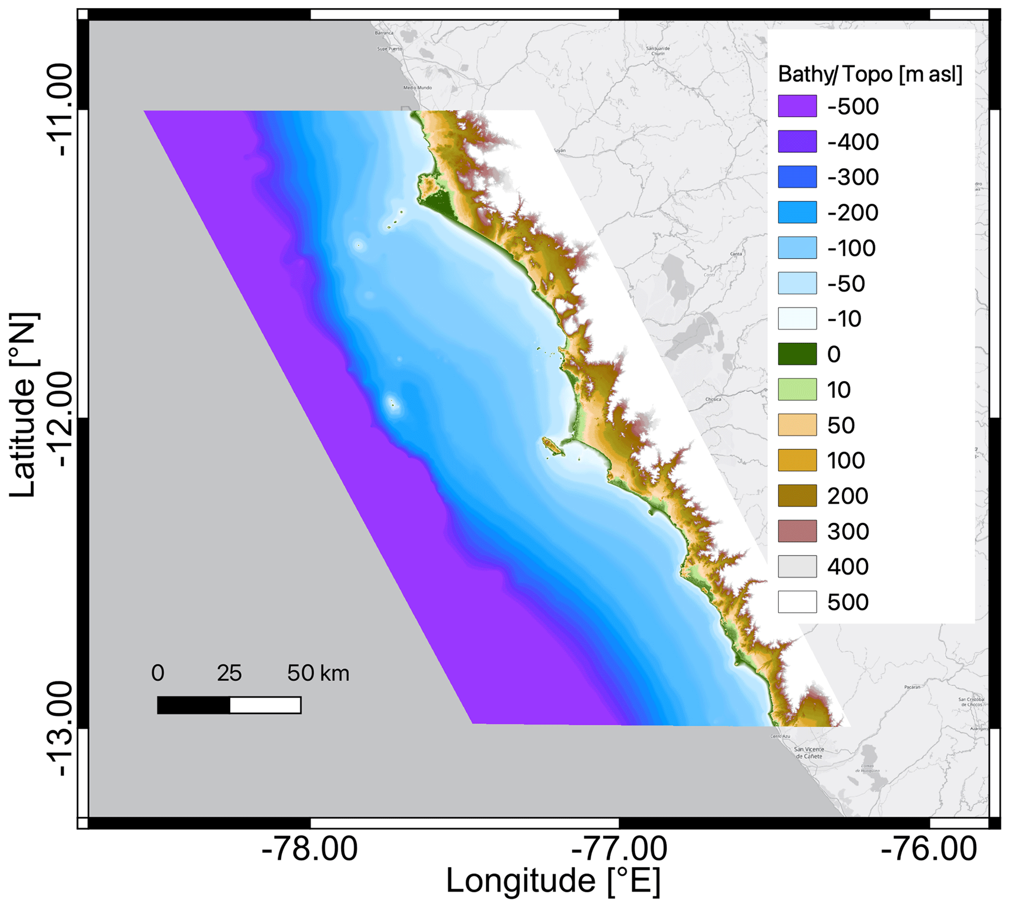
Figure 1 Bathymetry and topography in a section of the model domain with data processing by EOMAP. Values are given in meters relative to average sea level (m a.s.l.). Basemap © OpenStreetMap contributors 2021. Distributed under the Open Data Commons Open Database License (ODbL) v1.0.

3.3 Meshes

These numerical codes are based on two different meshes. In the case of Tsunami-HySEA, four levels of nested grids are used, and for TsunAWI, triangular meshes are required. To have similar resolutions along all domains between the numerical simulations that are compared, the triangular meshes are created from the nested grids with resolutions from 30 arcsec to about 1 arcsec (level 4). These meshes are shown in Figs. 2 and 3. In turn, the mesh resolution for TsunAWI is based on a criterion considering both water depth and bathymetry slope. A small section of the triangulation is displayed in Fig. 3.

Figure 2 Topography and bathymetry grids used for Tsunami-HySEA numerical simulations. In (a) the larger domain (level 1) has the coarsest resolution and the other three levels of the nested grids are shown with rectangles: level 2 (yellow), level 3 (green), and level 4 (see panel b since it is covered by the call station). S5, S7, and S9 stand for stations located around 10 m depth. More stations are located beyond this domain. In (b) grid level 4 stands for the domain with the highest spatial resolution. M1–M3 are the same virtual buoys used in Jimenez et al. (2013) and “call” refers to the buoy location in Callao (La Punta) according to the Intergovernmental Oceanographic Commission (IOC). Digital elevation model is from GEBCO Bathymetric Compilation Group (2019) and EOMAP. Values are given in meters relative to average sea level (m a.s.l.).

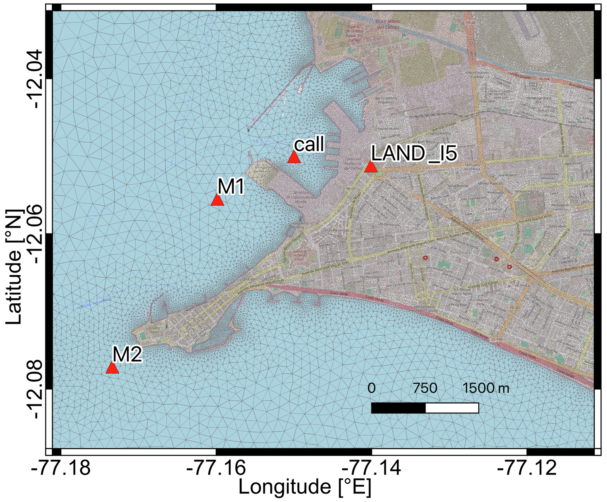
Figure 3 Small section of the triangular mesh used for TsunAWI simulations. The edge length of triangles ranges from 10 km in the deep ocean (beyond the scope of this image) to about 10 m in the highest resolved part. Also included are some of the locations used to analyze the time series. Basemap © OpenStreetMap contributors 2021. Distributed under the Open Data Commons Open Database License (ODbL) v1.0.

3.4 Model initialization

The event under consideration is the historic tsunami on 28 October 1746. We use the source parameters proposed by Jimenez et al. (2013) with slight depth adaptation for the center of the subfaults. Such depth at the center of each subfault was extracted based on the Slab2 Hayes et al. (2018). The source parameters are needed to generate initial conditions for the tsunami numerical simulations. In order to obtain initial conditions we used the Okada analytical formulations (Okada, 1985).

We compare the outcome of our modeling approach to their results. Our results are roughly similar, although bathymetry, topography data, and mesh resolution are different and complete agreement cannot be expected.

The source is shown in Fig. 4. It consists of five subfaults, each with lengths of 140 km, widths of 40 km, and with the given slip distribution with the moment magnitude M_w 9.0. An adaptation of the given source was needed to use the center of each subfault, estimated in this case at 24 km. Although the paper of Jimenez et al. (2013) considers a kinematic rupture, we restrict our investigation to a static seismic source for the sake of simplified consistency in the setups of the numerical models. More details on the source definitions are contained in Jimenez et al. (2013).

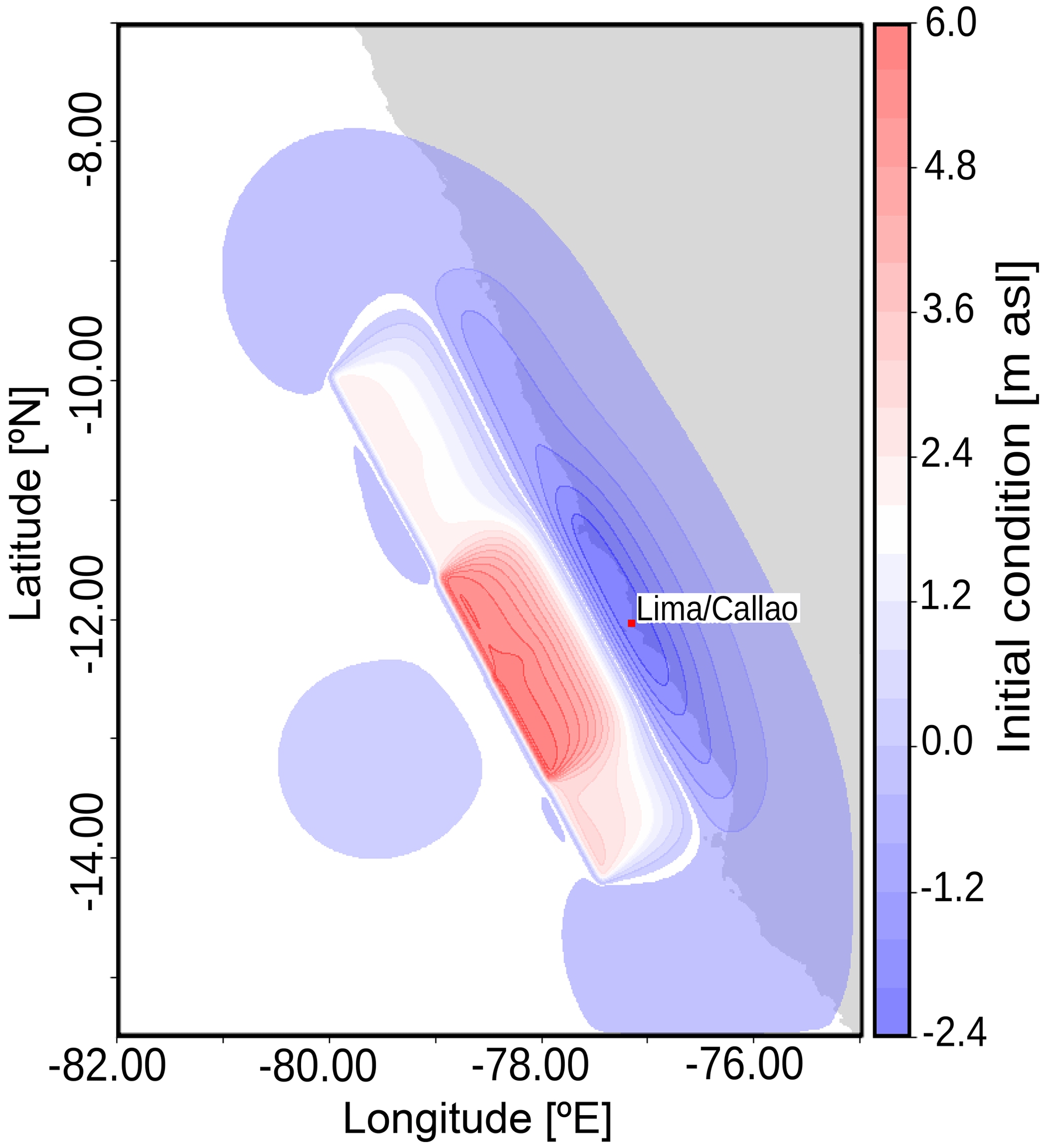
Figure 4 Initial conditions for the tsunami numerical simulations used by both models. Parameters modified from Jimenez et al. (2013). Values are given in meters relative to average sea level (m a.s.l.).

Starting from this initial sea surface elevation and zero velocity, we simulate the tsunami propagation and inundation for 4 h in real time. Besides the resulting inundation in the Lima/Callao region, we investigate and compare tide gauge records in virtual and real offshore positions as well as the temporal evolution in selected land points.

4 Comparison of model results

This section compares the simulation results of tsunami wave propagation and run-up modeling for the two numerical models presented above. The spatial and temporal fields show a detailed comparison of the simulation results. Some of the comparison results are given in the Appendix.

The Tsunami-HySEA and TsunAWI models are initialized with the same height fields and integrated over a 4 h time interval. The energy distribution indicated by the maximum wave amplitudes received during this period is shown in Fig. 5.

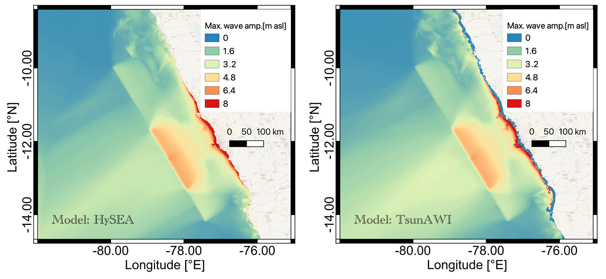
Figure 5 Maximum wave amplitude (in m a.s.l.) for a simulation of 4 h propagation time in the models Tsunami-HySEA (left panel) and TsunAWI (right panel). Basemap © OpenStreetMap contributors 2021. Distributed under the Open Data Commons Open Database License (ODbL) v1.0.

4.1 Inundation area

The historic event of 1746 resulted in considerable inundation in the Lima/Callao region (Jimenez et al., 2013). The flow depth in a part of the inundated area in the Callao region obtained by Tsunami-HySEA and TsunAWI is shown in Fig. 6. The extent corresponds qualitatively well with the result shown in Jimenez et al. (2013).

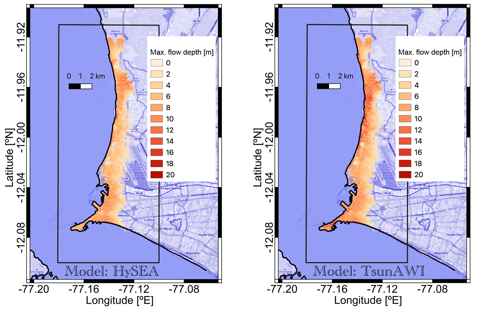
Figure 6 Maximum flow depth (in meters relative to topography) in the inundated area in Callao obtained by Tsunami-HySEA (left panel) and TsunAWI (right panel) for a Manning value of 0.015 and a simulation time of 4 h. The box indicates the area in which the inundation extent and inundation properties were calculated. Basemap © OpenStreetMap contributors 2021. Distributed under the Open Data Commons Open Database License (ODbL) v1.0.

The inundation extent, as well as the height distribution, depends on the bottom friction parameter in the inundated area. Both models use bottom friction parameterization in Manning form with a constant Manning coefficient throughout the domain. Results for Manning values (n) in the range between 0.015 and 0.06 are shown in Fig. 7. The inundation area (with a minimum flow depth of 1 cm) ranges from 21.29 km² (n=0.06) to 29.39 km² (n=0.015).

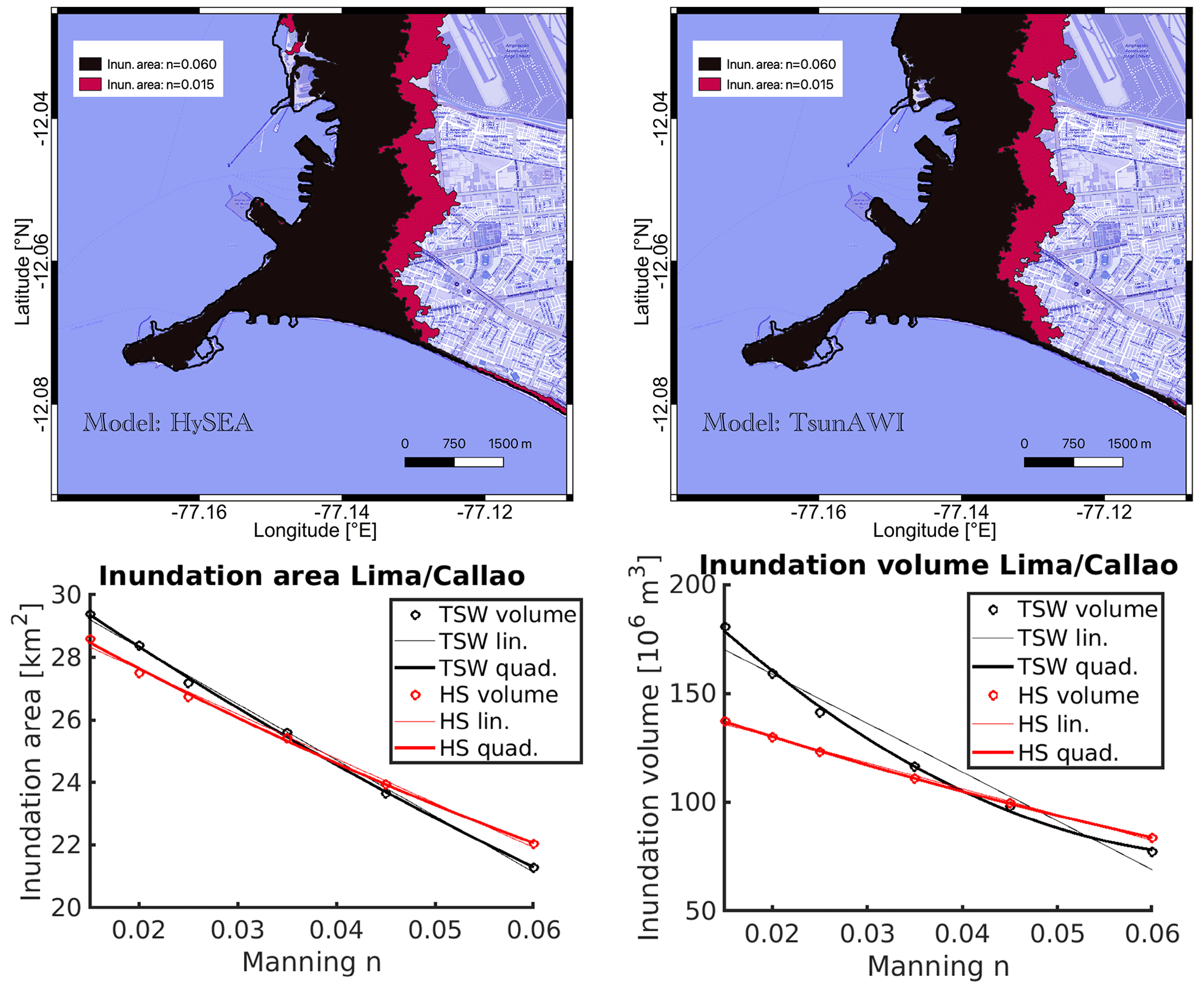
Figure 7 Upper panels: inundation extent for the smallest (n=0.015) and largest (n=0.06) Manning values used in this study obtained by Tsunami-HySEA (left side) and TsunAWI (right side). Lower panels: functional relationship of inundation area (km²; bottom left) and volume (10⁶ m³; bottom right) for the full range of Manning values used in this study. Linear and quadratic regressions are shown. Basemap © OpenStreetMap contributors 2021. Distributed under the Open Data Commons Open Database License (ODbL) v1.0.

The lower panels of Fig. 7 depict the regressions for inundation area (km²) and volume (10⁶ m³) concerning the Manning coefficient for both models. We consider the inundated land area in the box indicated in Fig. 6 and a minimum flow depth of 1 cm. The volume is estimated by integrating the maximum flow depth over the entire inundation area. The functional dependency for both models is quite similar, with gradual differences. Particularly, the volume obtained by TsunAWI for small Manning numbers is considerably more significant than the one determined by Tsunami-HySEA, since the numerical scheme in TsunAWI tends toward larger values of the wave height, especially in the nearshore range (see also Fig. A2). Over the full range of Manning values, we observe a reduction of 22.9 % in the inundation area for Tsunami-HySEA and 27.6 % for TsunAWI. Table A1 in the Appendix summarizes more quantities.

4.2 Time series comparison

We will continue the analysis of the results of the implementations of the two models by comparing the course of the wave height (see Fig. 8) and the horizontal velocity components (see Fig. 9) for the entire simulation period for stations M1–M3. A comparison of the tsunami wave amplitudes shows very high agreement with a correlation coefficient exceeding 0.96 for the two models. Note that the TsunAWI model shows somewhat greater instability in the solution. We can explain this because the Tsunami-HySEA model has higher stability in the frontal zones due to the stabilization of advection by schemes with flux limiters. A more interesting fact is a slight shift in the maximum amplitudes at the frequencies (close to 1 h) of the primary tsunami wave. This is especially noticeable at stations M2 and M3, which are the most distant from the initial disturbance source. So, for example, at station M3, the amplitude of the hourly frequency dominates in the Tsunami-HySEA model, and at frequencies close to 50 min, the amplitude in the HySEA model somewhat dominates. The picture is similar for the wave with frequencies of ∼37 and ∼42 min, where the amplitude maximum changes in one model or another. We also note that as we move away from the initial source of perturbation, there is a greater discrepancy between the two solutions at the time of the onset of the wave maximum. Some additional experiments show that the finite element model has a slightly higher phase propagation velocity than the finite volume model for long waves. This effect was also mentioned in the article by Maßmann et al. (2010) when comparing the tidal problem in the North Sea for different spatial approaches.

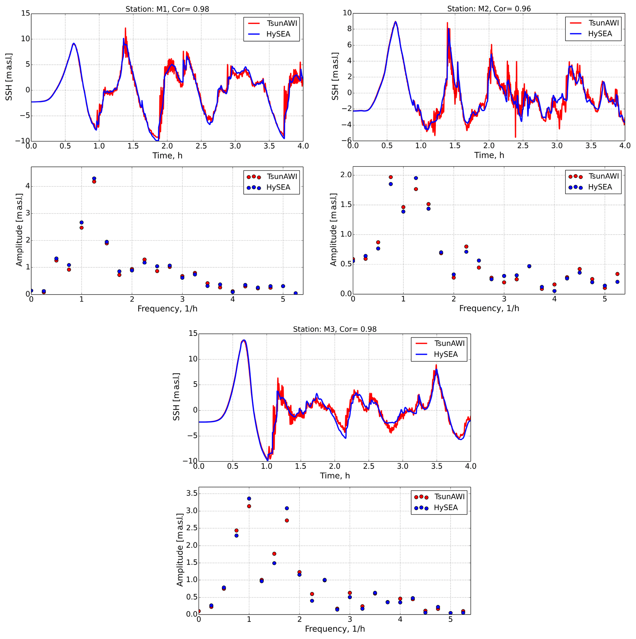
Figure 8 Wave amplitudes and their spectra for M1–M3 stations in the implementation of two models: Tsunami-HySEA and TsunAWI. SSH: sea surface height.

In comparing the horizontal velocity components shown in Fig. 9 at the same three stations, we see a high degree of similarity over the entire simulation period. The correlation coefficient of the two solutions at stations M1–M3 is 0.84, 0.95, and 0.94, respectively.

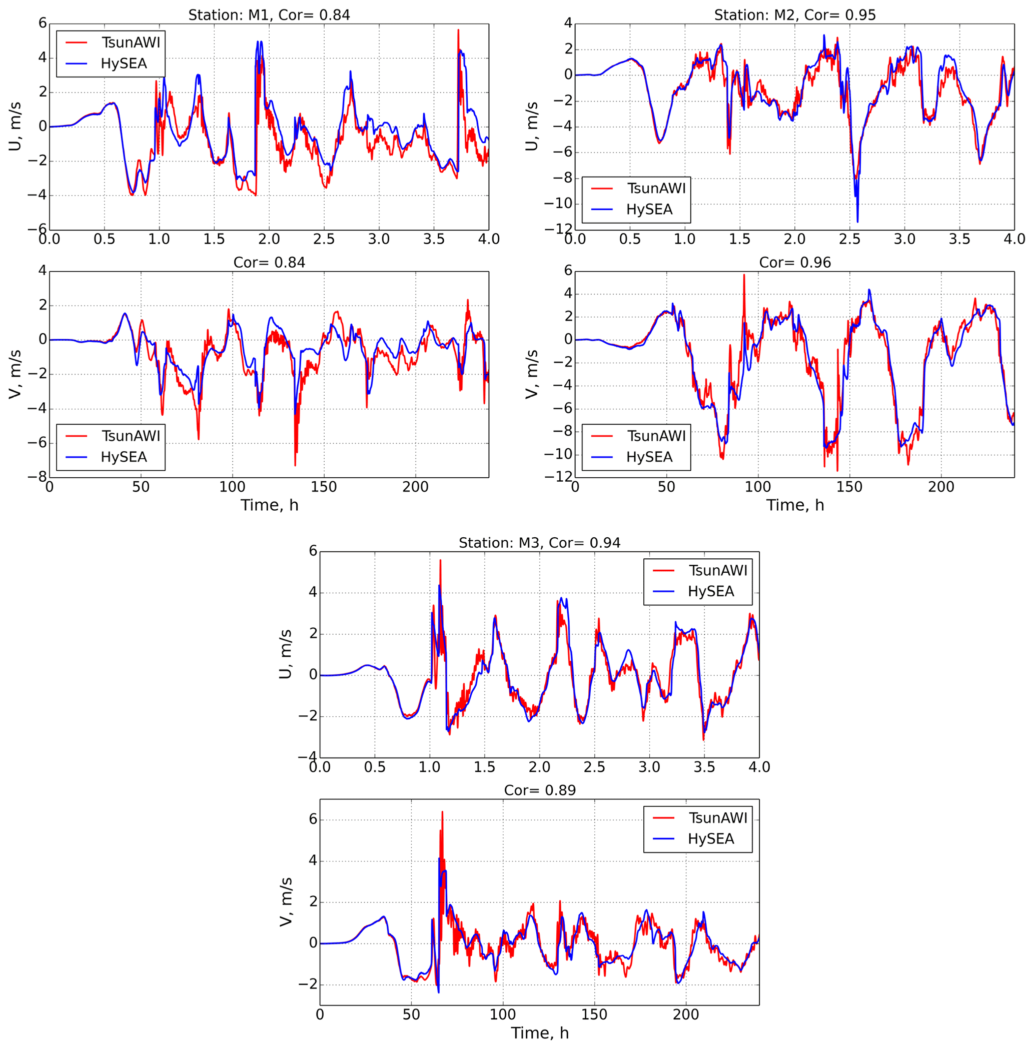
Figure 9 Comparison of horizontal velocity components at three stations, M1–M3, for two models: Tsunami-HySEA and TsunAWI. The top panel is the u component and the bottom is the v component.

The comparison of the two models presented in this section shows a high degree of agreement between the two solutions, which in turn allows us to choose the solution of TsunAWI for a more detailed analysis of the influence of nonlinearity on the behavior of the tsunami wave in the coastal zone and the inundation area.

5 Nonlinearity in the TsunAWI simulations

The system of Eqs. (1) and (2) contains three nonlinear terms: momentum advection, sea surface oscillations in the continuity equation, and nonlinear bottom friction. The analysis of the results of comparing the two models presented in the previous part of the work shows only minor differences in the redistribution of amplitudes at the main frequencies of the tsunami wave. This difference becomes noticeable only at the stations at the most remote distances from the source of the tsunami wave. This allows us to analyze the influence of nonlinear terms on the solution using the results of one (TsunAWI) numerical model.

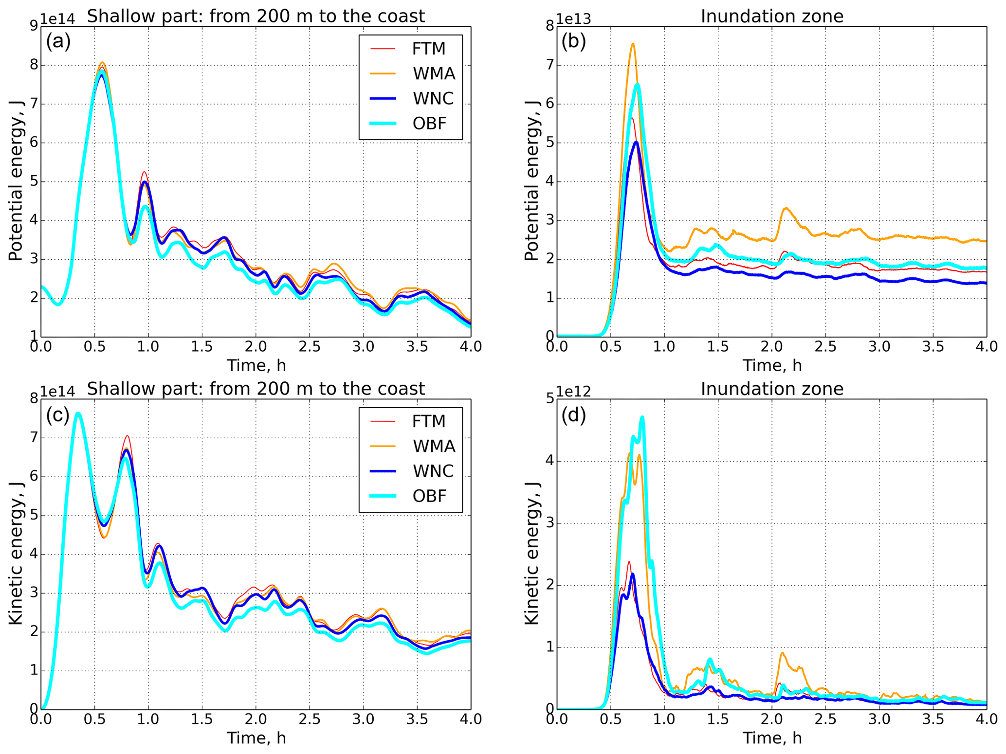
Figure 10 Potential and kinetic energies for four experiments for shelf zone and inundation area. Upper panels: potential energy; bottom panels: kinetic energy; left panels: shelf zone (from 200 m to coast); right panels: inundation area.

We performed four main nonlinear experiments on the propagation of a tsunami wave in the region of interest. The first experiment is the solution to the complete equations with all nonlinearity (full tsunami model (FTM)). The second experiment (without momentum advection (WMA)) is connected with disabling advection in the equations of motion, the second term in Eq. (1). In the third experiment, in the continuity equation (Eq. 2), the influence of the free-surface fluctuation on the total layer thickness (without nonlinearity in continuity (WNC)) was disabled in the velocity divergence term. Note that in the inundation area, as in all cases, we retain the total layer thickness h+ζ. Finally, in the fourth experiment (only bottom friction (OBF)), the nonlinearity in the equations is represented only by the bottom friction terms. An experiment analyzing the contribution to the nonlinearity of bottom friction with its sequential switching off is difficult to perform. Bottom friction is the only significant stabilizing factor in the numerical model for real applications. Due to complex morphometry and topography, the solution at the front of the wave is volatile and requires dissipation by bottom friction. In this regard, to evaluate the effect of the bottom friction coefficient, we additionally conduct a series of experiments with its different values and monitor the nature of the solution.

In the conclusion of this paper, using various coefficients of bottom friction, an analysis is made of the influence of nonlinear friction on the solution in the inundation zone.

We begin our analysis of the influence of nonlinear terms on tsunami wave propagation by comparing the potential and kinetic energies (Eq. 5) of the four experiments described above. The computational domain was divided into three subdomains: deep water (H>200 m), shelf (from 200 m to the coastline), and, in fact, the inundation area. For each of these regions, the potential and kinetic energies are calculated. Figure 10 shows the values of the terms of the total energy equation for the shelf zone and the inundated area. We note that in the deep water part of the region, the potential and kinetic energies have a practically insignificant difference in all four experiments. The difference between the terms of the energy equation in the shelf zone also turns out to be insignificant (left panel in Fig. 10) for the first incoming tsunami wave. Some visible differences in amplitude appear for secondary waves and waves reflected from the coastline.

Figure 10 (right panels) shows the values of potential and kinetic energies only in the inundation area. For this zone, the differences in the energy components are already quite significant. Thus, the potential energy of the WMA calculation exceeds the energy of the complete system of equations (FTM) by more than 35 %. Calculating equations without nonlinearity in the equation of continuity (WNC) shows an underestimation of the energy. In addition, an essential element of comparison is that in the WNC experiment, there is a slight phase shift in the onset of the maximum compared with the FTM experiment. The OBF experiment contains the general tendencies of the WMA and WNC experiments – an overestimated amplitude and a characteristic shift in the maximum of the first wave.

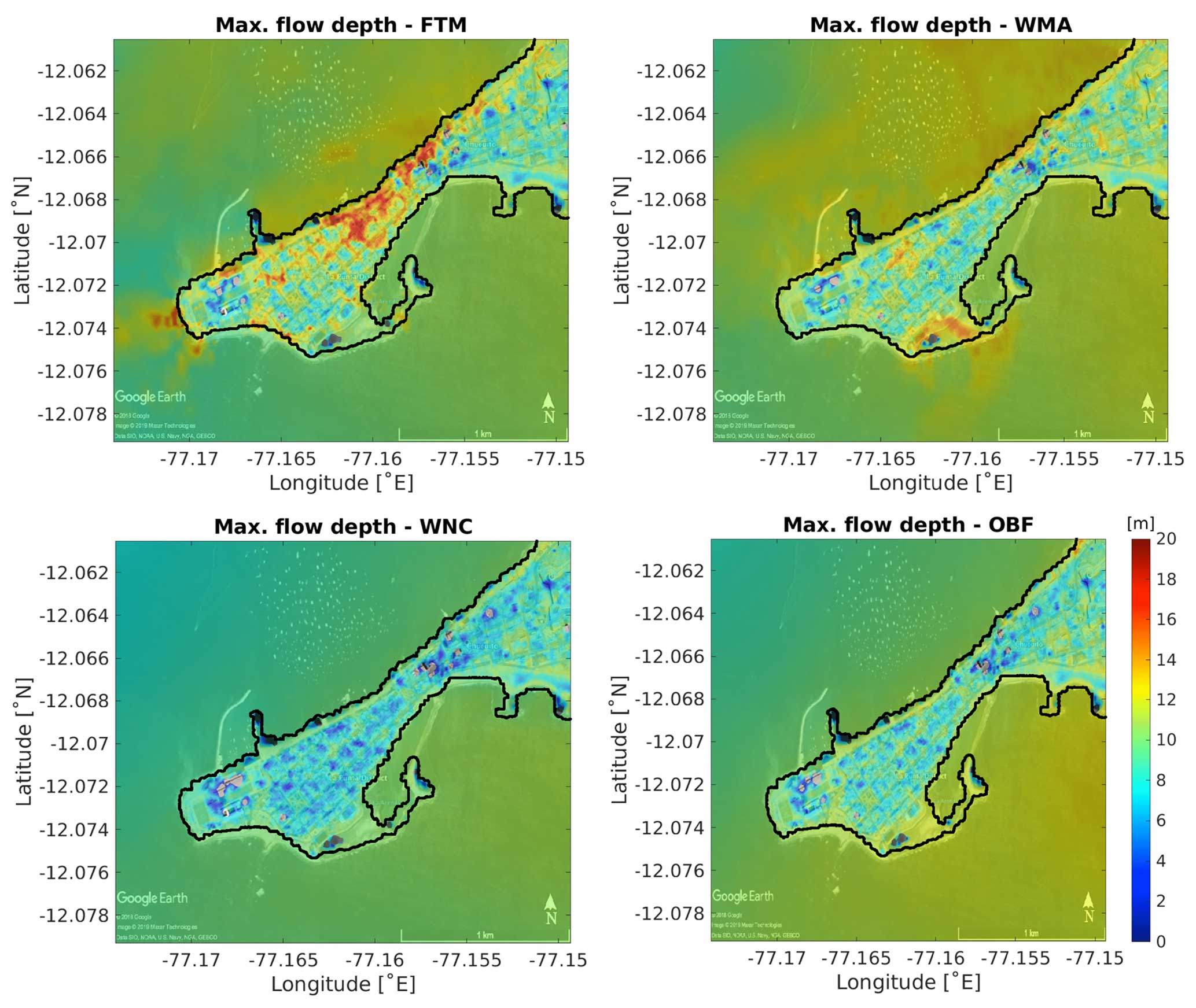
Figure 11 Maximum sea surface amplitude in the ocean (in m a.s.l.) and flow depth (in meters relative to topography) for the complete simulation period. Upper left panel: full model (FTM); upper right panel: without momentum advection (WMA); lower left panel: omitting nonlinearity in the continuity equation (WNC); lower right panel: only bottom friction (OBF). Basemap © Google Earth 2018.

The difference in kinetic energy in the coastal zone shows an even greater contrast. The absence of momentum in the equation of motion plays the leading role in kinetic and potential energies. The difference in amplitude compared with that of the basic experiment (FTM) reaches 50 %. At the same time, we note that the calculation with only bottom friction shows an even more significant energy contribution. This behavior is explained by a strong nonlinear character in the velocity field on the background of nonlinear bottom friction. The momentum advection in the equations works in the regions of high nonuniform velocities as a dissipation factor. For this reason, the basic experiment (FTM) has a lower energy contribution.

As shown below, considering nonlinear terms does not increase or decrease the horizontal velocity or elevation in the inundation area but completely changes the dynamic fields' structure.

We continue comparing the nonlinear effect by considering the dynamic characteristics: the maximum wave height and the velocity modulus in the Lima/Callao region. Figure 11 shows the spatial characteristics of the wave height for the four settings described above. As can be seen from the comparison, the level fields have significant differences both in amplitude and spatial structure. The wave height in the complete set has a local maximum in the narrowest part of the peninsula, with a wave height of up to 15 m. The WMA setup calculations characterize the local maximum on the opposite side of the peninsula and more significant amplitudes in the coastline zone. WNC calculations show underestimated tsunami wave amplitudes in the inundation area, with local maxima only along the coastline.

A remarkable feature is highlighted by analyzing the maximum horizontal velocity modulus in the same region. Figure 12 shows such fields for four settings. A characteristic feature of these fields is that in the absence of nonlinearity in the equation of momentum or continuity, there is a substantial intensification in the velocity along the coastline. The spatial structure of such filaments is in good agreement with the bathymetric features of the coastal zone (see Fig. 2). In the case of a complete task, the horizontal velocities are more uniform and have maxima only in front of building structures, where the level gradient is maximum. In the absence of advection of the WMA experiment, the field structure is significantly uneven, with velocities significantly exceeding the local maxima of the FTM problem. In the absence of nonlinearity in the continuity equation WNC, the velocity amplitudes in the inundation area are greatly underestimated and have only local maxima along the coast. In the absence of nonlinearity, except bottom friction (OBF experiment), the image sums up the calculation without one or another nonlinearity – significantly intensifying alongshore currents and increasing velocities locally in the inundation area.

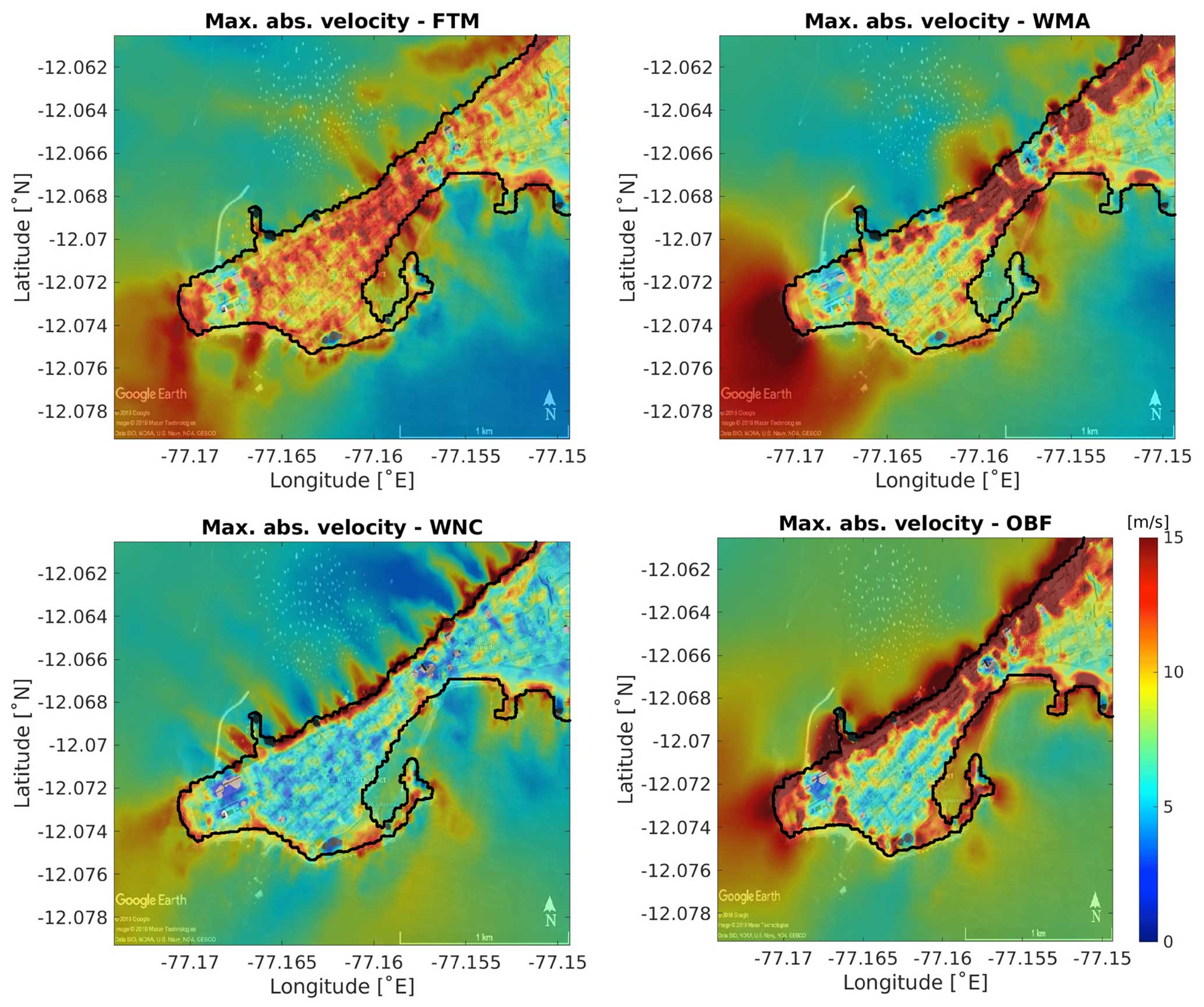
Figure 12 Maximum velocity modulus (in m s⁻¹) for the complete simulation period. Upper left panel: FTM; upper right panel: WMA; lower left panel: WNC; lower right panel: OBF. Basemap © Google Earth 2018.

Figure 13 presents the results of comparing the wave height at stations for four problem settings: FTM, WMA, WNC, and OBF. The positions of three stations (top left and right panels, as well as middle left panel) match those given in Jimenez et al. (2013): Callao (M1), La Punta (M2), and Costa Verde (M3). We also present the results for one station in the inundated area and two stations near coastlines to analyze the effect of nonlinearity (see Fig. 2 left and Fig. 3 left).

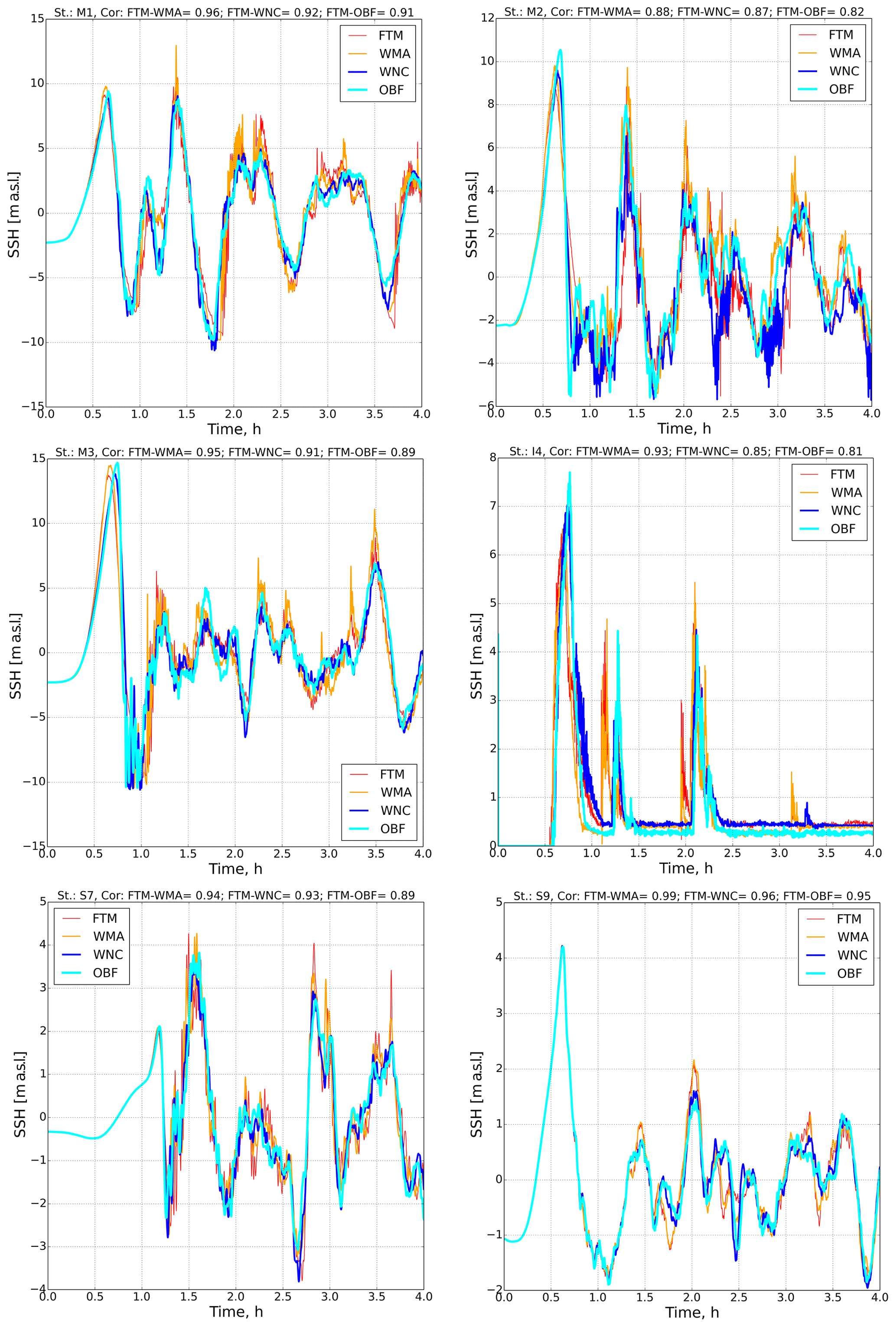
Figure 13 Time series of the sea surface elevation for the six points (M1, M2, M3, I4, S7, and S9) indicated in Fig. 2.

Comparison of the wave heights shows good agreement in the amplitude of the first wave at points M1 and M2 with the amplitude values in Jimenez et al. (2013) and are about 10 m. At the same time, at station M3, the wave amplitude in our implementation is about 6 m less, which can be explained by a slightly different initial disturbance and different topographic and bathymetric databases. So the depth of our bathymetry is more than 10 m, while in the above-cited article, it is only 4 m.

An analysis of the results reveals general patterns in studying nonlinear terms for stations M1–M3 offshore and coastal station I4. So, in the WNC experiments and OBF, the shape of the first incoming wave changes somewhat. In the absence of nonlinearity in the continuity equation, the waveform becomes flatter, which leads to a delay in the maximum of the first wave. At the same time, at stations located at a slightly small distance from the coast, i.e., S7 and S9, the effect of nonlinearity in the continuity equation is almost imperceptible. A similar shift in the maximum was also observed in the potential energy in the inundation area (see Fig. 10). It can be assumed that calculating a tsunami wave without nonlinearity in Eq. (2) changes the wave front in the entire simulated area. In addition, the absence of this kind of nonlinearity significantly reduces high-frequency disturbances. The waveform during the whole simulation period becomes smoother at coastal points. The lack of advection in the momentum equation (Eq. 1), in contrast, causes strong instability in the low-frequency spectrum, which once again confirms that momentum advection acts as a dissipation factor in this case.

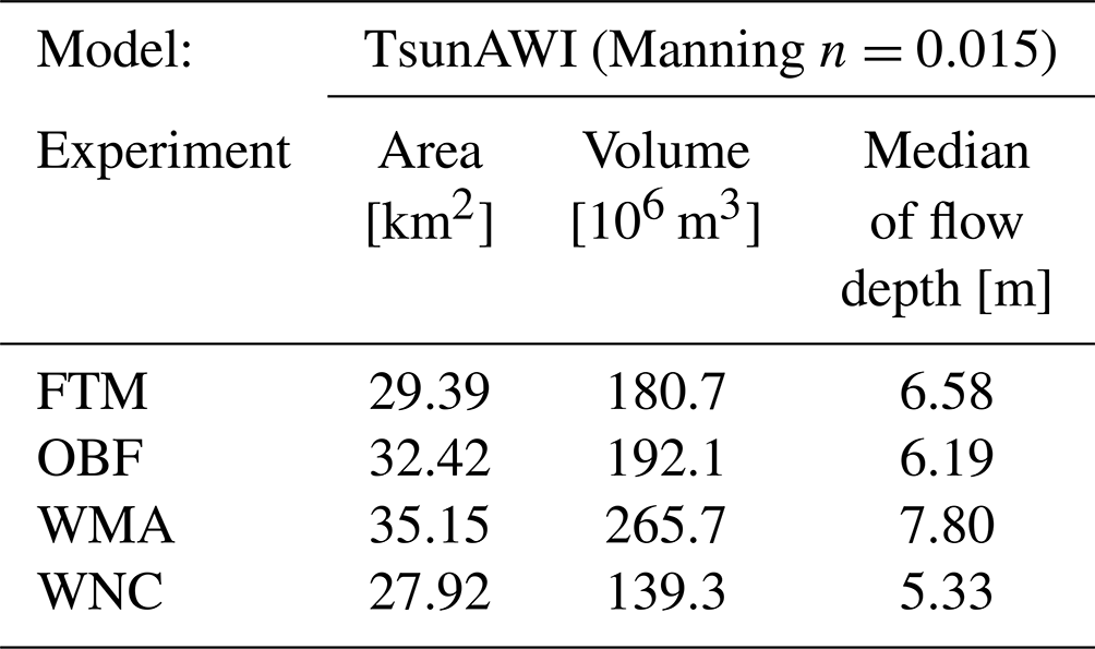
Finally, we summarize inundation properties for the nonlinearity investigation in Fig. 14 and Table 1. The figure shows the varying extent of the inundation area due to changes in the local velocity fields. The table highlights the different structures of the inundation process for the various setups. The simulation without momentum advection in the inundation area significantly increases potential energy (Fig. 10 top right panel). In the same figure, it becomes clear that the experiment keeping only the bottom friction (OBF) obtains a more considerable maximum value of potential energy than the full model (FTM); however, over time, these experiments swap roles, which is evident in the fact that OBF reaches a smaller median of maximum flow depth but a larger inundation area.

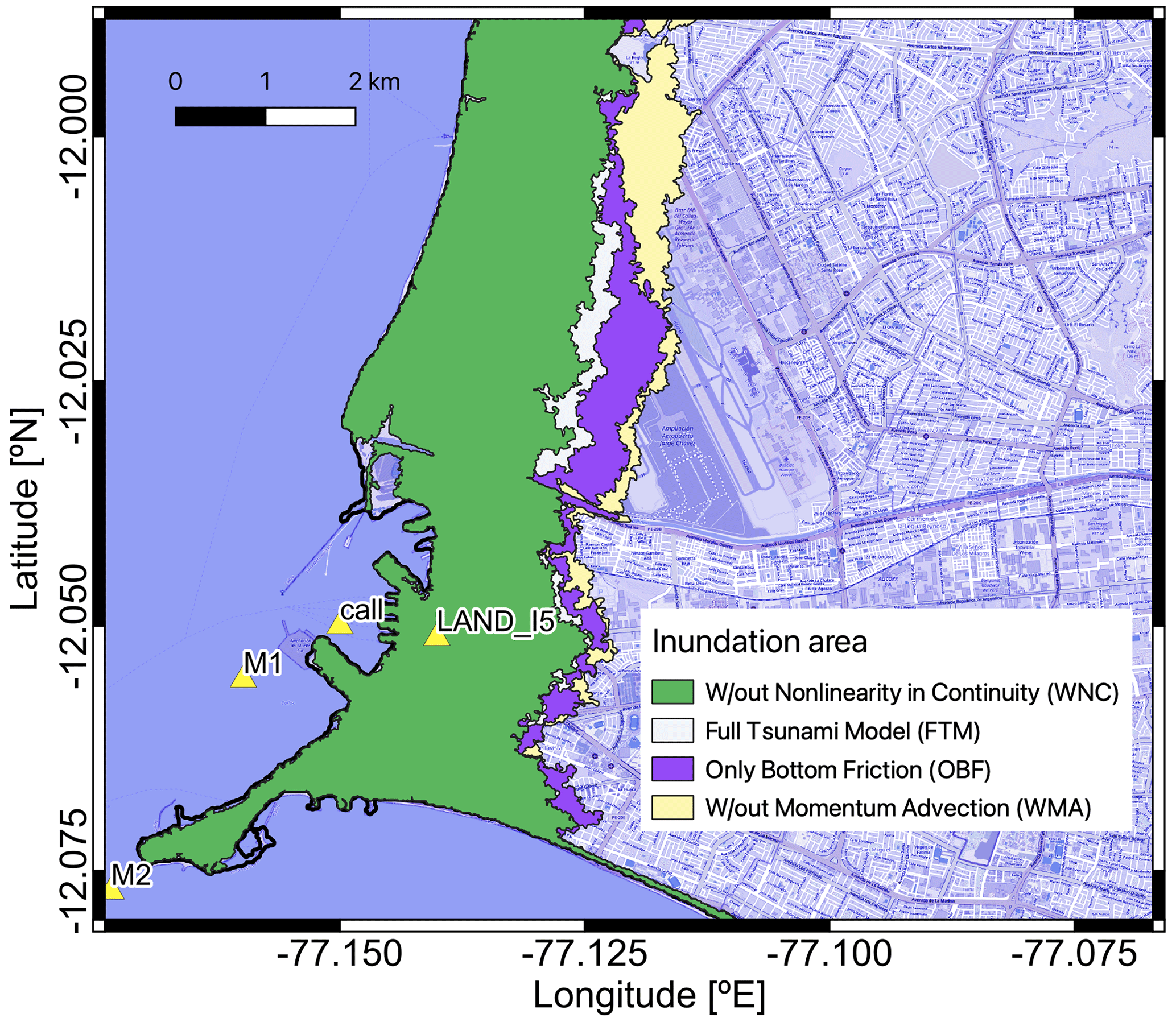
Figure 14 Inundation area obtained with TsunAWI for the experiments with the deactivation of different nonlinear terms. Basemap: © OpenStreetMap contributors 2021. Distributed under the Open Data Commons Open Database License (ODbL) v1.0.

Table 1 Properties of the inundation area obtained for different setups with regard to nonlinear terms (refer to Fig. 14). The values specify the inundation area (with more than 1 cm flow depth) in the bounding box shown in Fig. 6, the volume obtained by integrating the maximum flow depth over the whole inundation area, and the median of the maximum flow depth over the inundation area.

6 Conclusions

We examined the tsunami wave variations along the coast of Peru based on the 1746 earthquake scenario using two numerical models: Tsunami-HySEA and TsunAWI. For both models, it was found that there is a slight phase shift in the wave propagation velocity. Such a shift begins to manifest as the distance from the source of the tsunami wave increases. In the Tsunami-HySEA model, the leading edge propagation velocity slightly lags behind the wave velocity in implementing the TsunAWI model. We attribute this to the difference in dispersion errors in models with different spatial implementations. In the frequency spectrum, the wave maxima are redistributed at the main frequency of the tsunami wave for this event (∼1 h) and at nearby frequencies. Another difference between the two implementations is the more oscillatory nature of the dynamic characteristics of the TsunAWI model compared with Tsunami-HySEA. This is easily explained by the fact that limiters, in terms of the advection moment, were used in the latter model, a use which stabilizes the flow.

With an increase in the coefficient of bottom friction, the difference between the solutions of the two models, estimated by the total area and volume of water masses in the flood zone (see Fig. 7 and Appendix), begins to decrease, and at Manning coefficients of about 0.035, it practically disappears. With a further increase in the bottom friction coefficient, the model results again diverge somewhat. We explain this behavior of the solutions by the additional effect of using limiters of advective schemes in the Tsunami-HySEA model in inundation zones. Thus, with the minimum coefficient of bottom friction (Manning parameter 0.015) used in the calculations, the inundation area in the TsunAWI model is 29.39 km². In the Tsunami-HySEA model, it is 2.7 % less. The volume of water masses in the TsunAWI model exceeds the Tsunami-HySEA results by approximately 32 %. When the friction coefficient increases to 0.035, the difference in the inundated area decreases to 0.6 % and the difference in volume drops to 5.1 %. Otherwise, the outcomes of the two models have a high level of similarity.

Accounting for the nonlinear terms of the shallow water equations is numerically complex enough that they are often neglected in models designed to generate warning products remarkably quickly, such as in an early warning system. These terms are relatively insignificant in the deep ocean, and it may become acceptable to neglect them in computations. On the other hand, the contribution of nonlinearity becomes very significant when the tsunami wave reaches the coast and plays a very important role, especially in inundation.

A detailed assessment of the influence of nonlinearity on the solutions' behavior in the coastal and inundation areas has been conducted. The shallow water equations are considered in four formulations: complete equations (FTM); equations without momentum advection in horizontal velocity (WMA); in the absence of nonlinearity in the continuity equation, when velocity divergence is considered without taking into account free surface perturbations (WNC); and in the presence of only nonlinearity in bottom friction terms (OBF).

A preliminary assessment of the bathymetry of the area showed that the sharp bottom slope is located at a considerable distance from the coastline. The shelf zone extends for several kilometers behind it. It could be expected that, in this case, the nonlinearity in the continuity equation would be the maximum difference in the solution. A comparison of the results of wave height measurements at stations along the coast showed that the WNC experiment slightly shifts the beginning of the maximum, making the incoming tsunami wave flatter and, at the same time, practically does not change the wave amplitude. The lack of impulse advection (WMA) introduces the most significant changes in the amplitude of the incoming wave. Apparently, this is due to the orientation of the initial momentum of the free surface perturbation, which initially causes a significant shift in the velocity fields in space with a rather complex configuration of the coastline in the study area. We also attribute a significant increase, almost twofold, in the wave amplitude at coastal stations in the WMA experiment to a decrease in the dissipation of the solution, the role of which is partially played by the momentum advection term.

An analysis of the spatial solution in the flood zone without one or another nonlinearity introduces cardinal differences between the level and velocity fields from the complete problem statement. In the WNC experiment, the maximum wave amplitude on the coast is significantly underestimated, while in the WMA calculation the flood maxima are overestimated.

Overall, we confirm that nonlinearity plays a decisive role in estimating inundated areas, wave heights, current speeds, and the spatial structure of inundation maps. These factors should be considered when conducting numerical simulations of tsunami hazards to ensure that the solution persists in the nearshore and inundated zones.

Appendix A: More results on the model comparison

A1 Inundation properties

For the sake of completeness of the analysis, we will summarize some more results regarding the model comparison in this Appendix. The inundation area for a given Manning value is quite similar for the two numerical models. This is consistent with a similar assessment conducted for the Chilean cities Valparaíso, Viña del Mar, and Coquimbo (Harig et al., 2022). Nevertheless, the spatial height distribution varies considerably locally. An example for n=0.020 is shown in Figs. A1 and A2. Especially in the area close to the coastline, TsunAWI results in larger wave heights than Tsunami-HySEA, with even more significant differences for small Manning values. This is exemplified in the intersect comparison shown in the lower panel of Fig. A2.

The inundation properties also depend on the shape of the bottom relief in the offshore domain. In the case of Lima and Callao, the nearshore bathymetry is characterized by a very gentle slope in the bottom relief as shown in Fig. A3. Larger values of the bottom gradient are only present in some specific locations, which partly project on the local features of the maximum wave amplitude.

A collection of all inundation polygons is shown in Fig. A4. The variation in inundation distance to the coastline may vary considerably depending on the bottom relief but is quite consistent for the two models.

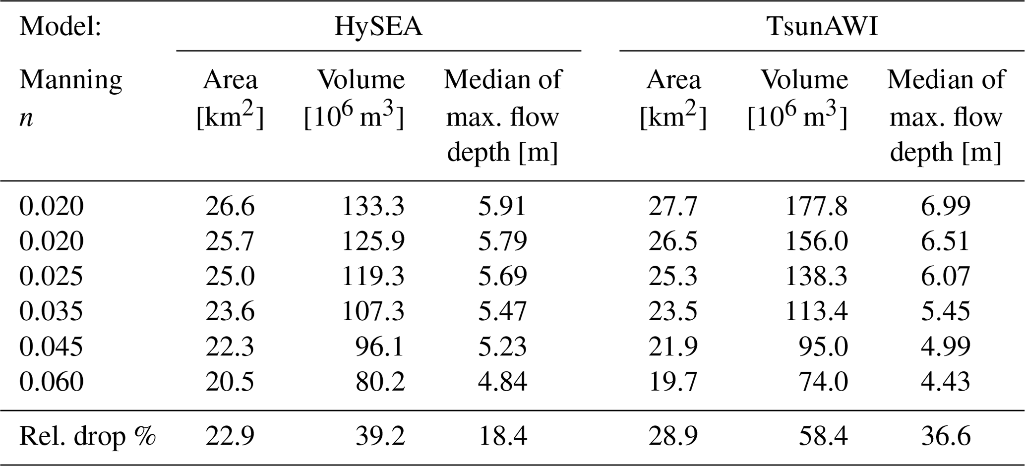
Table A1 summarizes some major inundation properties for both models and all Manning values as shown in Fig. 7. Here a minimum flow depth of 1 cm defines the inundation extent. The corresponding values for a minimum flow depth of 1m are listed in Table A2. Tables A1 and A2 also include the relative reduction in the quantities over the full Manning value range, and we observe an inundation area reduction between 20 % and 30 % for the two models, with TsunAWI obtaining generally larger values (both in estimates and reductions). The largest differences between the models occur in the volume estimates. Here TsunAWI determines considerably larger values probably due to larger fluctuations and larger wave heights determined by this model close to the coast (see also Fig. A2). This difference is also visible in the medians of the maximum wave height.

The velocity (modulus) distributions, together with the maximum values in the intersect, are shown in Fig. A5. The general structure is very similar in the nearshore range as well as on land, with regional variations. Peak values are somewhat larger for Tsunami-HySEA.

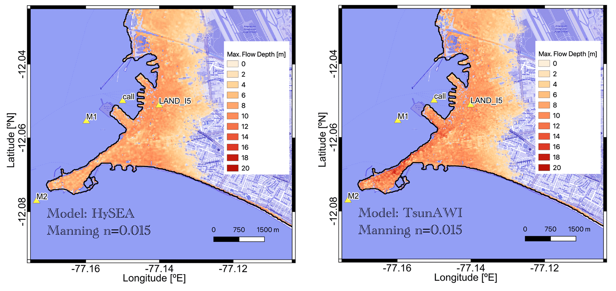
Figure A1 Maximum flow depth (in meters relative to topography) in La Punta and the Callao port area for simulations of 4 h propagation in Tsunami-HySEA (left panel) and TsunAWI (right panel). Basemap © OpenStreetMap contributors 2021. Distributed under the Open Data Commons Open Database License (ODbL) v1.0.

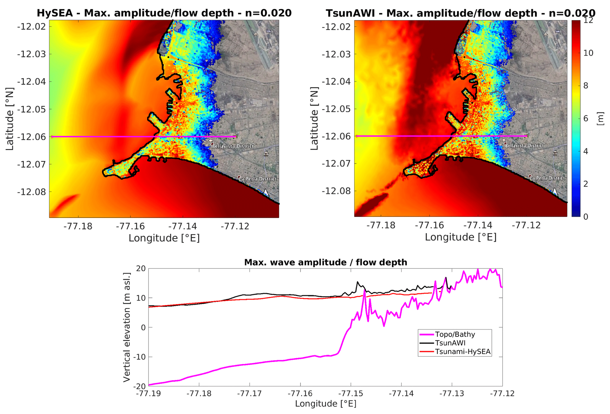
Figure A2 Upper panels: maximum wave amplitude in the ocean (in m a.s.l.) and flow depth on land (in meters relative to topography) in the Callao port area. Lower panel: maximum wave amplitude projected to the intersect shown in the upper panels. All results obtained for Manning value of 0.020. Basemap © Google Earth 2018.

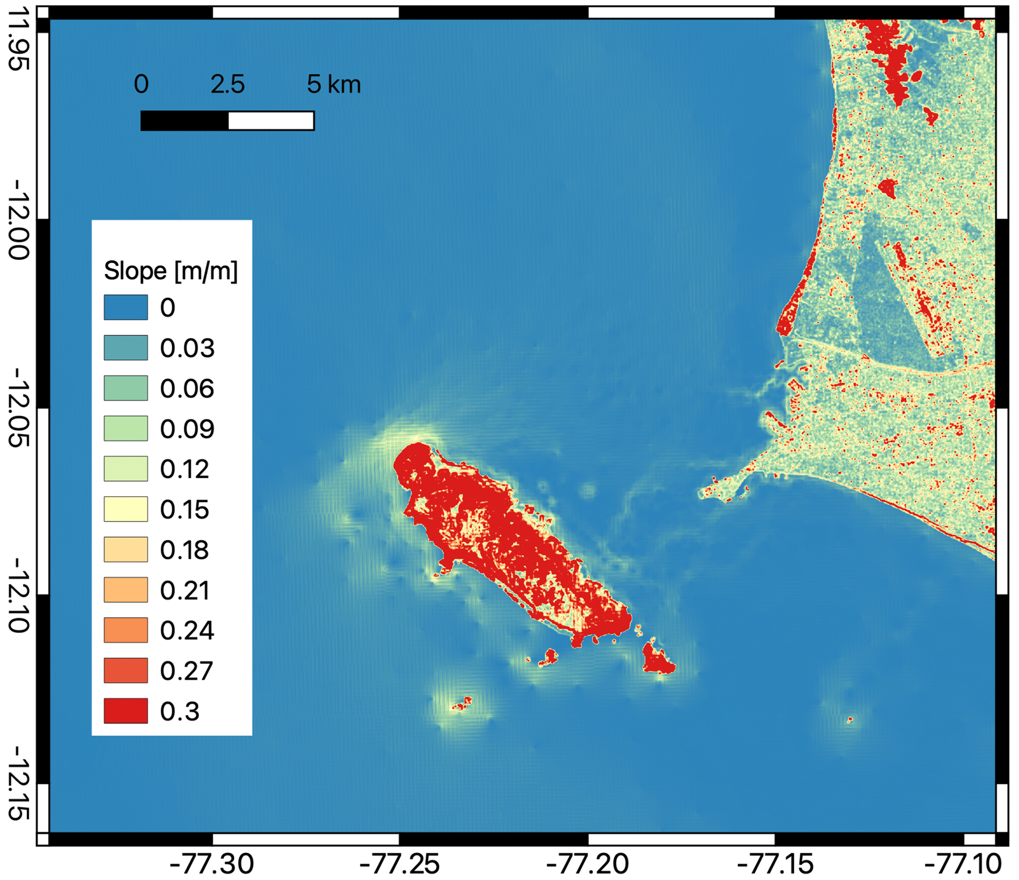
Figure A3 Slope in bathymetry and topography in the Callao port area. This gradient is determined from the data shown in Fig. 1.

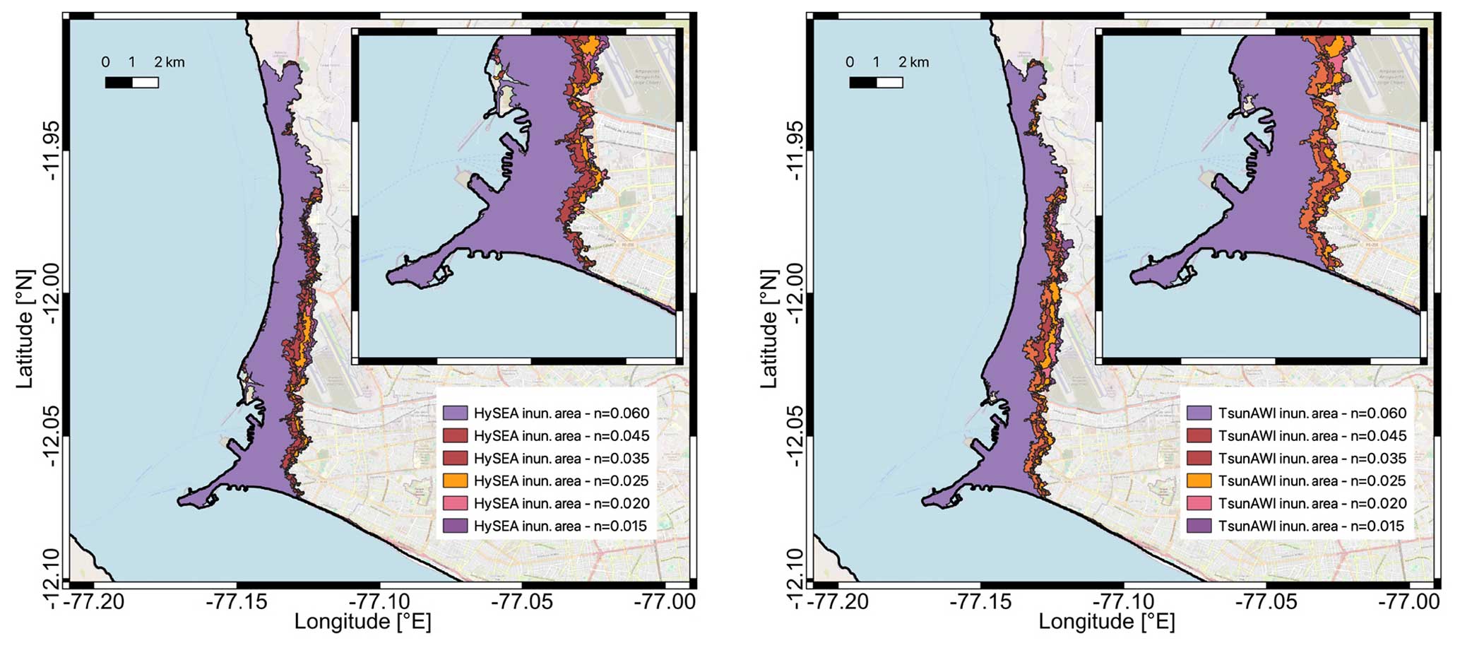
Figure A4 Inundation area with minimum flow depth of 1 cm for all Manning values obtained with Tsunami-HySEA (left panel) and TsunAWI (right panel). Basemap © OpenStreetMap contributors 2021. Distributed under the Open Data Commons Open Database License (ODbL) v1.0.

Figure A5 Upper panels: maximum absolute velocity (in m s⁻¹) in the Callao port area obtained with Tsunami-HySEA (upper left panel) and TsunAWI (upper right panel). Manning value in both models is 0.020. Lower panel: maximum absolute velocity projected to the intersection shown in the upper right panel. As a reference, the bottom relief is overlaid in gray color. Basemap in (a) and (b): © Google Earth 2018.

Table A1 Properties of the inundation area obtained with both models for the full range of Manning values. The numbers specify the inundation area (with a minimum flow depth of 1 cm) in the bounding box shown in Fig. 6, the volume obtained by integrating the maximum flow depth over the whole area, and the median of the maximum flow depth in the whole inundation area. The last row contains the relative reduction in all quantities over the Manning range as shown in Fig. 7.

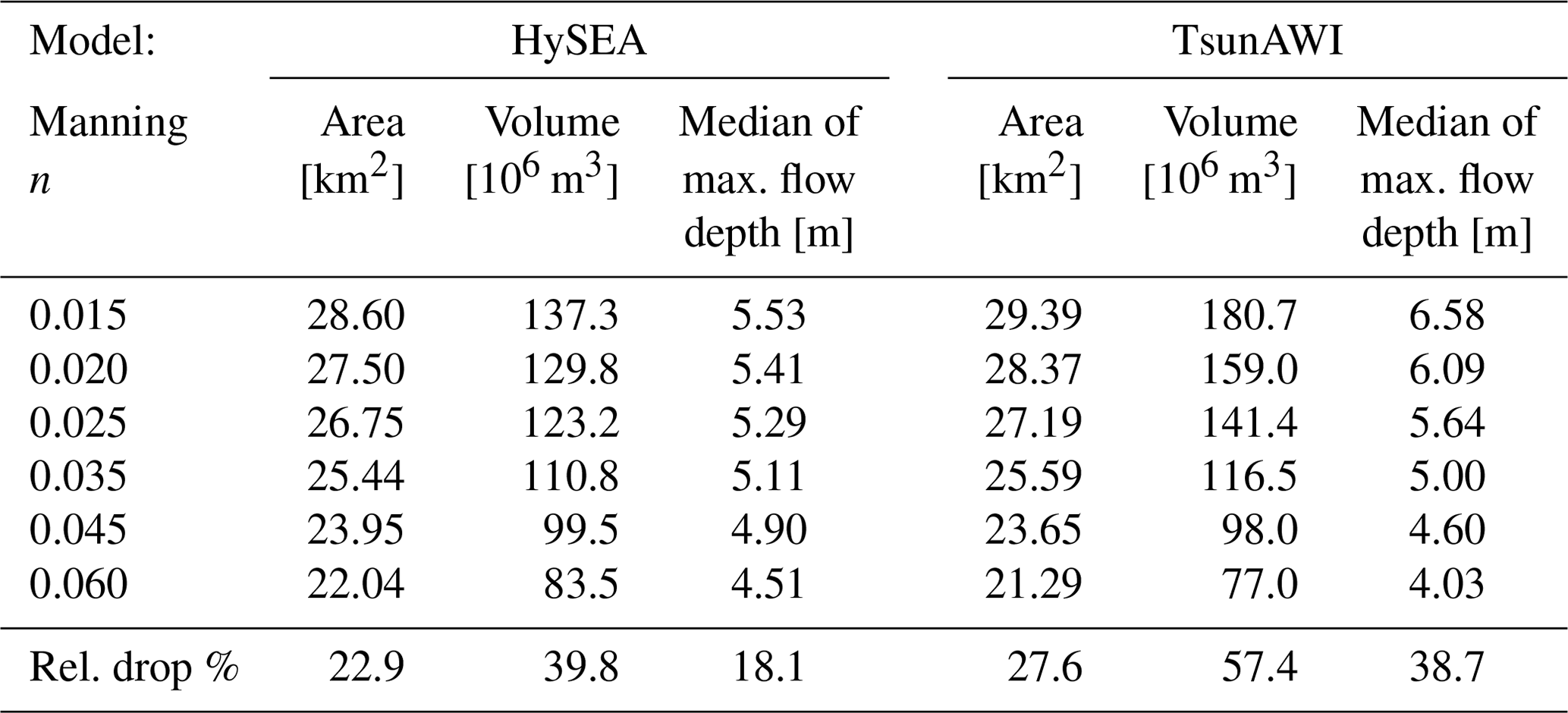
Table A2 Inundation quantities as indicated in Table A1, but obtained using a minimum flow depth threshold of 1 m.