the Creative Commons Attribution 4.0 License.
the Creative Commons Attribution 4.0 License.
 | 10 Apr 2024
Interannual variations in the seasonal cycle of extreme precipitation in Germany and the response to climate change
Madlen Peter
Henning W. Rust
Uwe Ulbrich
Annual maxima of daily precipitation sums can be typically described well with a stationary generalized extreme value (GEV) distribution. In many regions of the world, such a description does also work well for monthly maxima for a given month of the year. However, the description of seasonal and interannual variations requires the use of non-stationary models. Therefore, in this paper we propose a non-stationary modeling strategy applied to long time series from rain gauges in Germany. Seasonal variations in the GEV parameters are modeled with a series of harmonic functions and interannual variations with higher-order orthogonal polynomials. By including interactions between the terms, we allow for the seasonal cycle to change with time. Frequently, the shape parameter ξ of the GEV is estimated as a constant value also in otherwise instationary models. Here, we allow for seasonal–interannual variations and find that this is beneficial. A suitable model for each time series is selected with a stepwise forward regression method using the Bayesian information criterion (BIC). A cross-validated verification with the quantile skill score (QSS) and its decomposition reveals a performance gain of seasonally–interannually varying return levels with respect to a model allowing for seasonal variations only. Some evidence can be found that the impact of climate change on extreme precipitation in Germany can be detected, whereas changes are regionally very different. In general, an increase in return levels is more prevalent than a decrease. The median of the extreme precipitation distribution (2-year return level) generally increases during spring and autumn and is shifted to later times in the year; heavy precipitation (100-year return level) rises mainly in summer and occurs earlier in the year.
- Article
(9581 KB) - Full-text XML
- BibTeX
- EndNote


Climate change has been identified as the cause of increasing risks from meteorological extreme events affecting almost all areas of the economy, nature, and human life, and those will be even more endangered in the future (Pörtner et al., 2022, and the references therein). One of the main targets of current and future generations is to avoid further changes and to develop adaptation strategies to reduce risks and burdens.
While climate change can be measured very reliably for the surface temperature, for other variables like extreme precipitation the connection is not yet clear. For regions with good data availability, it has already been shown that frequency and intensity of heavy precipitation have likely increased on the global scale (Seneviratne et al., 2021). Furthermore, climate projections show that future extreme precipitation will continue to intensify (e.g., Pörtner et al., 2022; Rajczak et al., 2013). Since the consequences of heavy precipitation are extensive and can lead to different threats and damages, for example, due to flash floods, river floods, mudslides or soil erosion, an accurate assessment of extreme precipitation changes is crucial for an adequate adaptation. The potential risk due to extreme precipitation is not only dependent on its magnitude, but it also can be related to a change in its seasonal cycle. For example, a shift of strong precipitation from summer to spring leads to an increased flood risk due to a larger likelihood of strong rainfall and snowmelt occurring at the same time (Vormoor et al., 2015; Teegavarapu, 2012). Furthermore, crop losses may rise, since plants are more vulnerable during earlier growing stages (Rosenzweig et al., 2002; Zeppel et al., 2014; Derbile and Kasei, 2012).
Analyses of extreme precipitation in Germany for different seasons have already been done(Zolina et al., 2008; Łupikasza, 2017; Fischer et al., 2018; Fischer et al., 2019; Zeder and Fischer, 2020; Ulrich et al., 2021). Zolina et al. (2008) and Łupikasza (2017) analyzed quantiles of daily precipitation sums separately for the seasons DJF, MAM, JJA and SON, while Fischer et al. (2018, 2019) used available data more efficiently by modeling monthly maxima of daily precipitation sums for all months simultaneously. This approach has been proven to lead to more robust and reliable results than considering months separately. Ulrich et al. (2021) extended this method by including different durations to efficiently estimate intensity–duration–frequency curves. Furthermore, Zeder and Fischer (2020) analyzed the effect of climate change on seasonal extreme precipitation and found a positive connection to the northern-hemispheric temperature rise. In our approach we combine the simultaneous modeling of available data for all months with interannual variations, thus accounting for potential changes in the seasonality due to climate change and natural variability. Here, we point out that when referring to interannual variations, we are not addressing differences between successive years, but rather the trend over the entire observation period, which could be potentially non-linear.
Extreme value statistics (EVS) (e.g., Coles, 2001; Bousquet and Bernardara, 2021) are used to quantify the magnitude and occurrence probabilities of these seasonally–interannually varying extremes. EVS have been applied in many different research fields (e.g., Katz et al., 2002; Ferreira et al., 2017; Szigeti et al., 2020; Arun et al., 2022). One way to analyze extremes is the block maxima approach, where the observations are divided into blocks with equal lengths. The probability distribution for the maxima of these blocks is represented by the generalized extreme value (GEV) distribution. Instead of considering annual maxima of precipitation, which are frequently used in risk assessment, we take a monthly block size to resolve the seasonal cycle. Contrary to a stationary approach with an individual extreme value model for each calendar month, we take advantage of the smooth variations in the probability distributions of the block maxima across adjacent calendar months. Because of the periodic nature of the seasonal changes, a series of harmonic functions is an appropriate choice for describing the corresponding variations in the GEV parameters. This modeling strategy has already been widely applied (e.g., Méndez et al., 2007; Rust et al., 2009; Galiatsatou and Prinos, 2014; Fischer et al., 2019; Min and Halim, 2020). It has been shown to provide more accurate monthly and annual return levels (quantiles of the GEV) (Fischer et al., 2018).
Interannual variations in precipitation have been shown to be associated with its natural variability (e.g., Willems, 2013), increased air temperatures (Trenberth et al., 2003; Westra et al., 2013, 2014), and other effects influencing large-scale atmospheric circulations and precipitation characteristics (Pinto et al., 2007, 2009; Davini and d’Andrea, 2020; Detring et al., 2021). Most of these effects are highly non-linear, and their roles are difficult to quantify. Here, we use time as a proxy to combine those different unknown effects. One possibility to model non-linear interannual changes is polynomial regression (e.g., Kjesbu et al., 1998; Mudelsee, 2019; Bahrami and Mahmoudi, 2022). Orthogonal polynomials are used to reduce multicollinearity and to improve the parameter estimation (Shacham and Brauner, 1997). Here, we use Legendre polynomials up to an order of 5 to describe the variations across years. On the one hand, this enables the reflection of changes potentially associated with climate change, and, on the other hand, this allows for modeling of natural variability in extreme precipitation. The concept of using higher-order Legendre polynomials has also been applied to assess spatial variations (Ambrosino et al., 2011; Rust et al., 2013; Fischer et al., 2019). As the seasonal and interannual covariates are conceptually equal, we combine both approaches. Additionally, interactions between the covariates allow the seasonal cycle to change across years.
The goal of this paper is to assess the performance of the seasonal–interannual modeling with a special attention to a flexible shape parameter ξ. This parameter is difficult to estimate as it interferes with the scale parameter (Ribereau et al., 2011) and requires long records for reliable results (Papalexiou and Koutsoyiannis, 2013). Nevertheless, it describes the behavior of the very rare events and consequently plays an important role for assessing extreme precipitation changes. Furthermore, the possible impact of climate change on the seasonal cycle of extreme precipitation is analyzed. We formulate three research questions to be addressed in this study.
- RQ1
-
Can a model with interannual variations better represent the observations than a seasonal-only model?
- RQ2
-
How important is a flexible shape parameter to reflect recorded variations?
- RQ3
-
How does climate change affect the seasonal cycle of extreme precipitation in Germany?
We carry out this investigation for observations from Germany with more than 500 long (≥ 80 years) records, presented in Sect. 2. The seasonal–interannual modeling is described in Sect. 3. Model selection and validation tools are covered in Sect. 4. The gain of modeling seasonal–interannual variations with respect to a just seasonal model (RQ1) and the importance of a flexible shape parameter ξ (RQ2) are assessed in Sects. 5 and 6. The impact of climate change on the seasonal cycle of heavy precipitation (RQ3) is tackled in Sect. 7. Finally, we discuss the results in Sect. 8.
A dataset of almost 5700 rain gauges measuring daily precipitation amounts (DWD, 2021) is provided by the German Meteorological Service (Deutscher Wetterdienst, DWD) via the continuously updated Open Data Server (DWD, 2022). Those observation stations are set up according to the WMO guidelines (WMO, 1996). The daily sums of precipitation are obtained from amounts accumulated between 05:50 and 05:50 UTC of the following day and have been checked for spatial consistency (DWD, 2021).
For investigating long-term trends a sufficiently long time series is crucial; thus, we only consider the most recent stations with at least 80 years of observations lasting until 31 December 2021. We allow for missing values and larger gaps of several consecutive years, often occurring for the years of the second world war. The 519 stations fulfilling the mentioned criteria are depicted in Fig. 1; the color coding shows the station's altitude. The locations are not homogenously distributed in space: some areas are closely covered, while for other areas, for example, in the east of Germany or in the state of Saarland in western Germany, long time records which are still being updated are missing. The common time period for all 519 observation records covers the years from 1941 to 2021. The four stations Krümmel (1 January 1899 until 31 December 2021), Mühlhausen/Oberpfalz-Weihersdorf (1 January 1931 until 31 December 2021), Rain am Lech (1 January 1899 until 31 December 2021) and Wesertal-Lippoldsberg (1 January 1931 until 31 December 2021) are highlighted in Fig. 1 and will be discussed exemplarily in this study. We have selected these stations as they are characterized by different changes in seasonality (see Sect. 7) represented by divergent model setups (see Sect. 4.1). Additionally, their interannual changes are more pronounced than for other stations. We consider monthly maxima of daily precipitation sums while months with less than 27 measured days are discarded from the analysis.
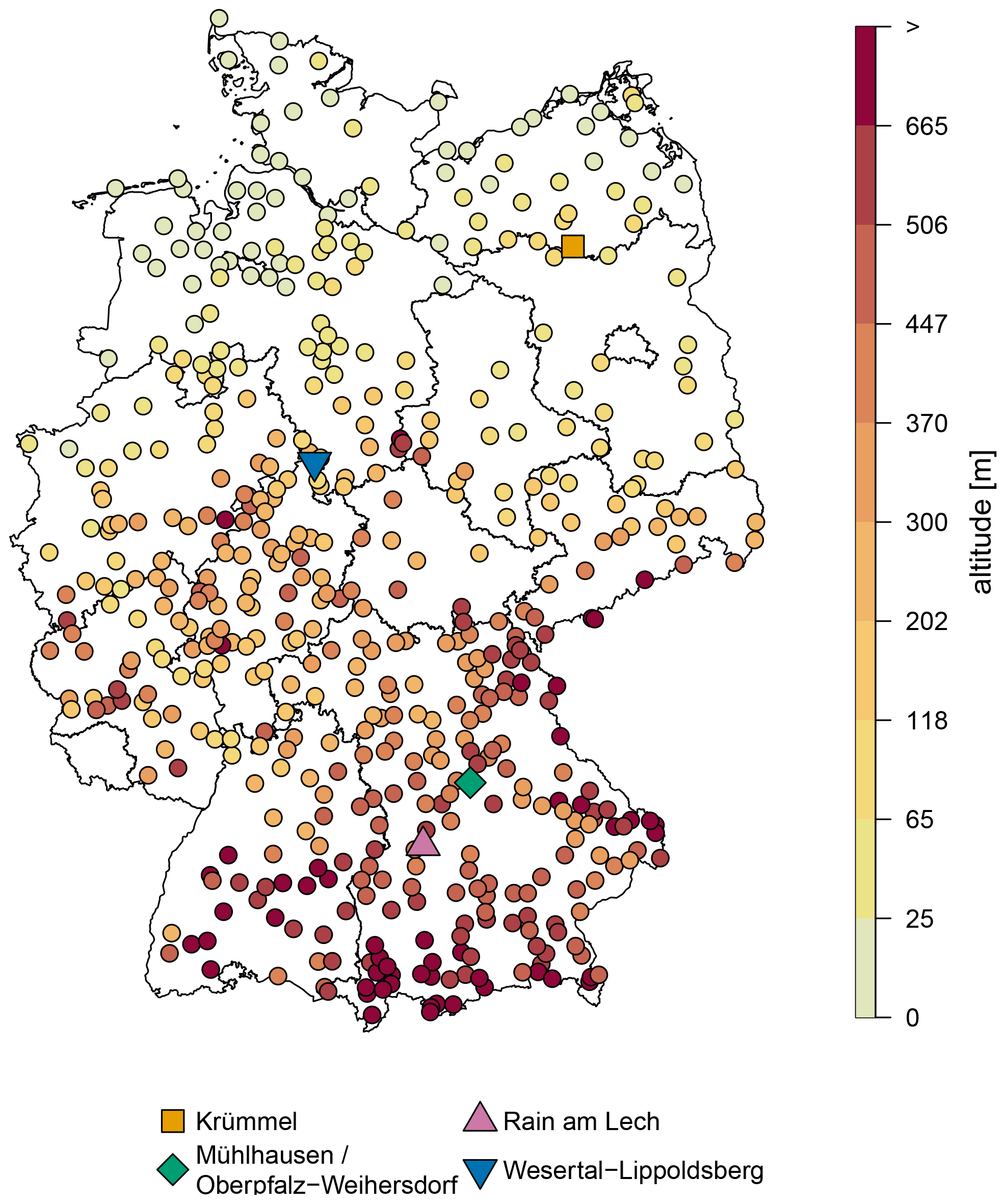
Figure 1The 519 long stations covering at least the years from 1941 to 2021. Station altitude [m] is encode with colors. Additionally, the locations of stations Krümmel (orange rectangle), Mühlhausen/Oberpfalz-Weihersdorf (green rhombus), Rain am Lech (violet triangle pointing up) and Wesertal-Lippoldsberg (blue triangle pointing down) are depicted.
In order to describe the changes in seasonality of extreme precipitation, we build a statistical model. This can be done with concepts of extreme value statistics (EVS), which are widely explored and applied in different scientific fields (e.g., for the financial sector, Gilli and Këllezi, 2006; Gkillas and Katsiampa, 2018; or for geosciences, Yiou et al., 2006; Naveau et al., 2005; Ulrich et al., 2020; Fauer et al., 2021; Moghaddasi et al., 2022; Jurado et al., 2022). One major strategy in EVS is the block maxima approach leading to an asymptotic model for extreme values: the generalized extreme value (GEV) distribution, briefly described in the following.
3.1 Block maxima approach
For a sequence of independent and identically distributed (iid) random variables , the block maxima are defined as
The Fisher–Tippett–Gnedenko theorem (FTGT) (Coles, 2001) states that for a sufficiently large block size n, the probability distribution function (PDF) of the block maxima can be well described either with the Gumbel, the Fréchet or the Weibull distribution. The three families can be combined into the generalized extreme value (GEV) distribution:
with . This distribution has three parameters: location , specifying the position of the PDF; scale σ > 0, defining the width of the PDF; and shape , characterizing the behavior of the upper tail. The value of ξ determines the type of extreme value distributions (: Gumbel; ξ > 0: Fréchet; ξ < 0: Weibull).
The choice of the appropriate block size is dependent on the nature of the considered random variable (Embrechts et al., 1997; Rust, 2009). Studies (e.g., Rust et al., 2009; Maraun et al., 2009) show that a block size of 1 month is already sufficiently large for extreme precipitation in the mid-latitudes. Others confirm the choice of monthly maxima for the considered datasets by using Q–Q plots (Fischer et al., 2018, 2019). The advantage of a higher temporal resolution of the maxima series makes it possible to analyze the seasonal cycle of extreme precipitation. This requires independent block maxima of successive months. However, this assumption can be violated if two monthly maxima belong to the same precipitation event, e.g., if one maximum occurs at the end of the month and the second one at the beginning of the next month. For the given records, about 0.6 % of the monthly maxima have been registered at successive days. Since the percentage is low, we neglect temporal dependencies and assume independent monthly maxima.
In the frame idea of vector generalized linear models (VGLMs Yee, 2015), we describe the variation of GEV parameters as linear functions depending on different variables. The variations throughout the course of the year are captured in Fischer et al. (2018) and are extended to a seasonal–spatial variation of extreme precipitation in Fischer et al. (2019). Ulrich et al. (2020) applied spatial variations to a duration-dependent GEV. Additionally, a change in the GEV parameters with other meteorological variables – e.g., temperature and the El Niño–Southern Oscillation (ENSO) index (Villafuerte et al., 2015), the North Atlantic Oscillation (NAO) index (Golroudbary et al., 2016), or an index of synoptic airflow (Maraun et al., 2011) – has been accomplished by various authors. In this study the seasonal and interannual variations are in focus. For each of the three GEV parameters, we build a linear model as shown here in a conceptional way for μ:
where g is a link function – for μ the identity function g(μ)=μ , for σ the logarithm g(σ)=ln (σ) and for ξ the logarithm with an offset of 0.5 ; μ0 denotes the constant intercept (offset); the second term denotes the direct effects of a covariate Xi, e.g., seasonal or interannual; and the third term denotes the interactions between different dimensions (indicated by i and j), e.g., seasonal and interannual.
3.2 Modeling seasonality
To account for the periodic nature of the seasonal cycle, the dependence of GEV parameters on the months can be described with a series of harmonic oscillations with amplitude A and a phase α. For the first harmonic oscillation (h=1) the location parameter μ can be written as
with the months in the year, ct the center of the tth month given in days starting from 1 January and the angular frequency of Earth's rotation.
To describe the oscillation Eq. (4) in the framework of a linear model, we use a linear combination of sine and cosine,
with the coefficients a and b defining the amplitude A and the phase α as
and
The harmonic series for location,
with indicating the order of harmonic function, approximates an arbitrary periodic function (Priestley, 1992).
3.3 Modeling interannual variation
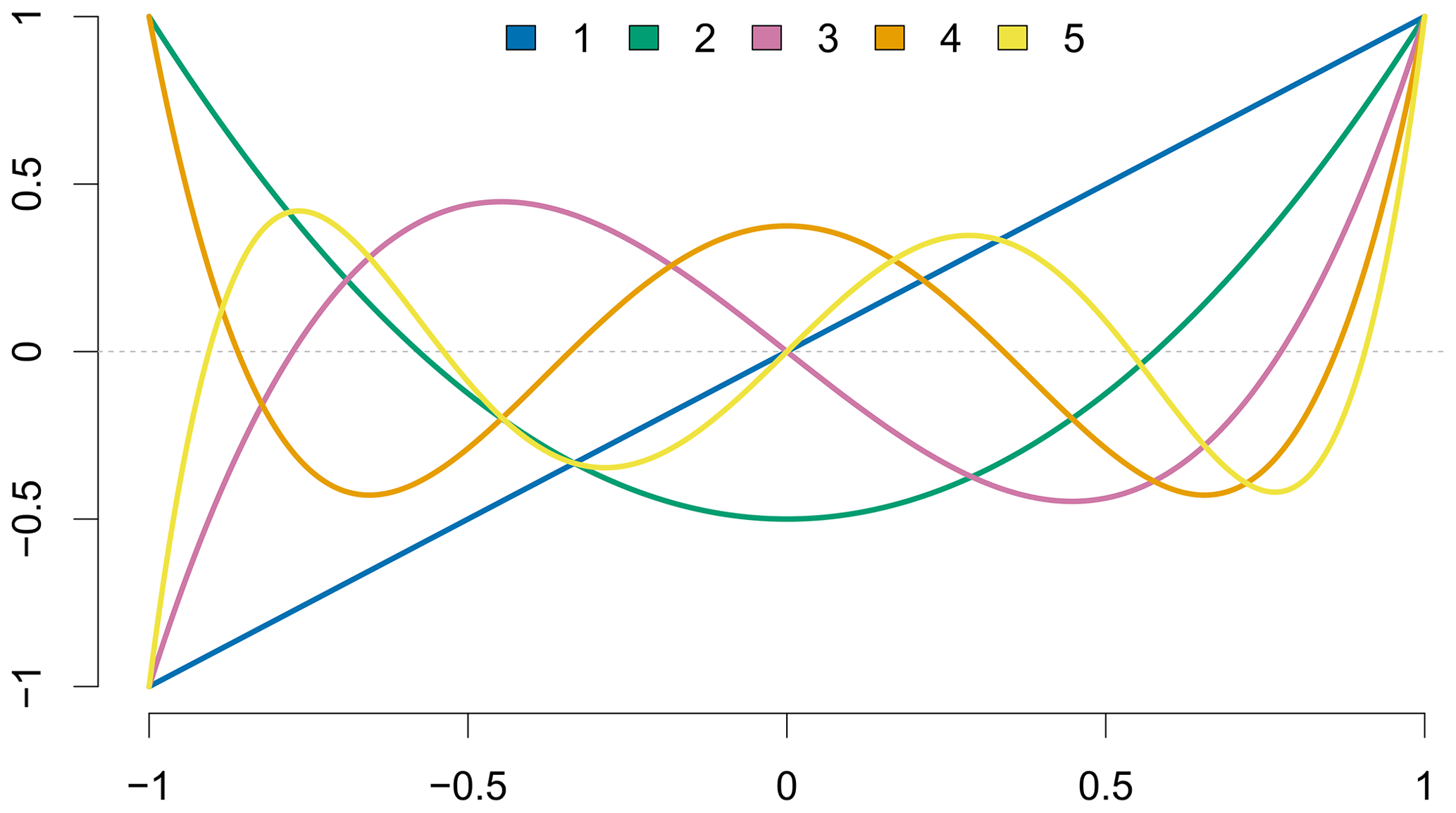
To capture interannual variations, polynomials typically provide a good approximation. With orthogonal polynomials such as Legendre polynomials, we avoid dependence between terms which have proven useful for modeling spatial variations (Rust et al., 2013; Fischer et al., 2019). We adopt this approach here to describe interannual variations. For the location parameter μ this reads
with indicating the order of Legendre polynomial P and Y the transformed year of the observation. The transformation of the time axis needs to be done since Legendre polynomials are only defined on . For that we use
with Y′ being the respective year and denoting the first/last year of the record. This transformation has been done for each station separately depending on its observation period. We exemplify the Legendre polynomials up to order 5 in Fig. 2.
3.4 Modeling the interannual variation of seasonality
We focus on the interannual changes in the seasonal cycle, which can be incorporated into the statistical model using interactions between the seasonal and interannual terms in the predictor of the vector generalized linear model. It can be thought of as the amplitude and phase of the seasonal cycle changing in time.
Using Eq. (6) with coefficients a(Y)=a Pi(Y) and b(Y)=b Pi(Y) being modulated by time-dependent Legendre polynomials P(Y), the amplitude A varies with the square of the Legendre polynomials P(Y): with the compact support on interaction of harmonics with a linear change with years P1(Y) leads to a quadratic change for the squared amplitude A2 and thus to an interaction term a sin (ω ct) P1(Y)+b cos (ω ct) P1(Y) with decreasing amplitude on and increasing amplitude on [0,1] as illustrated in Fig. 3 (top row, with b=0 for simplicity). The following rows of Fig. 3 show the corresponding interaction terms for P2(Y) (middle) and P3(Y) (bottom).
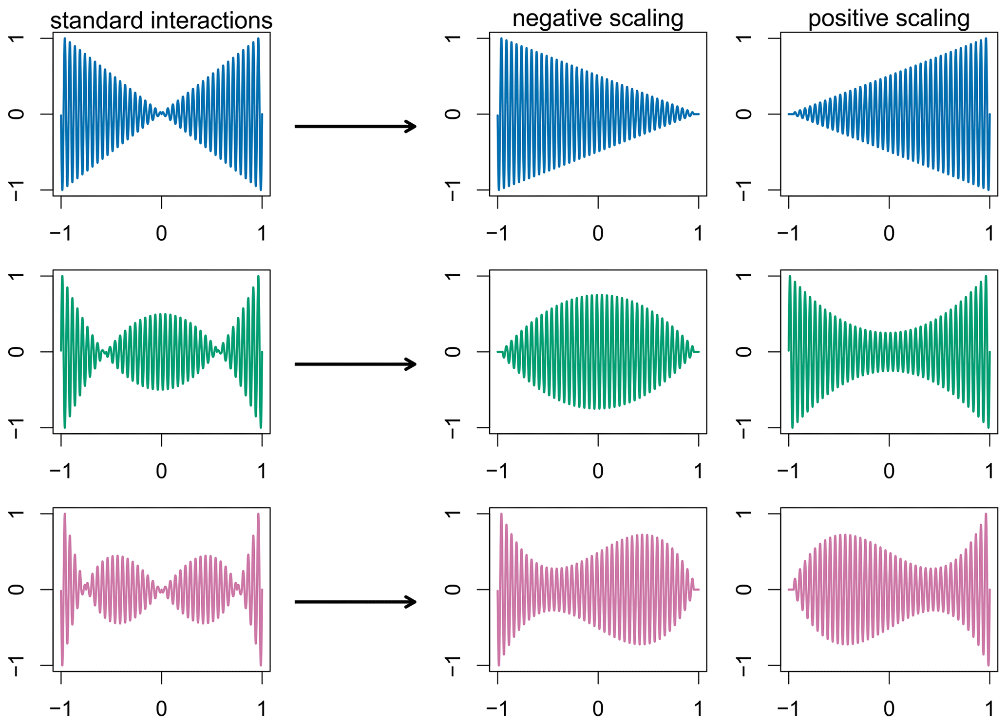
Figure 3Standard interaction terms (left-hand side) between the first-order sine and the Legendre polynomials of order 1 (top row, orange), order 2 (middle row, green) and order 3 (bottom row, red). A negative and a positive scaling of the Legendre polynomials lead to the desired interaction terms (right-hand side).
To avoid the bipartite behavior we use two transformations of the Legendre polynomials: and , such that and .
The transformed Legendre polynomials are illustrated in Fig. 4.
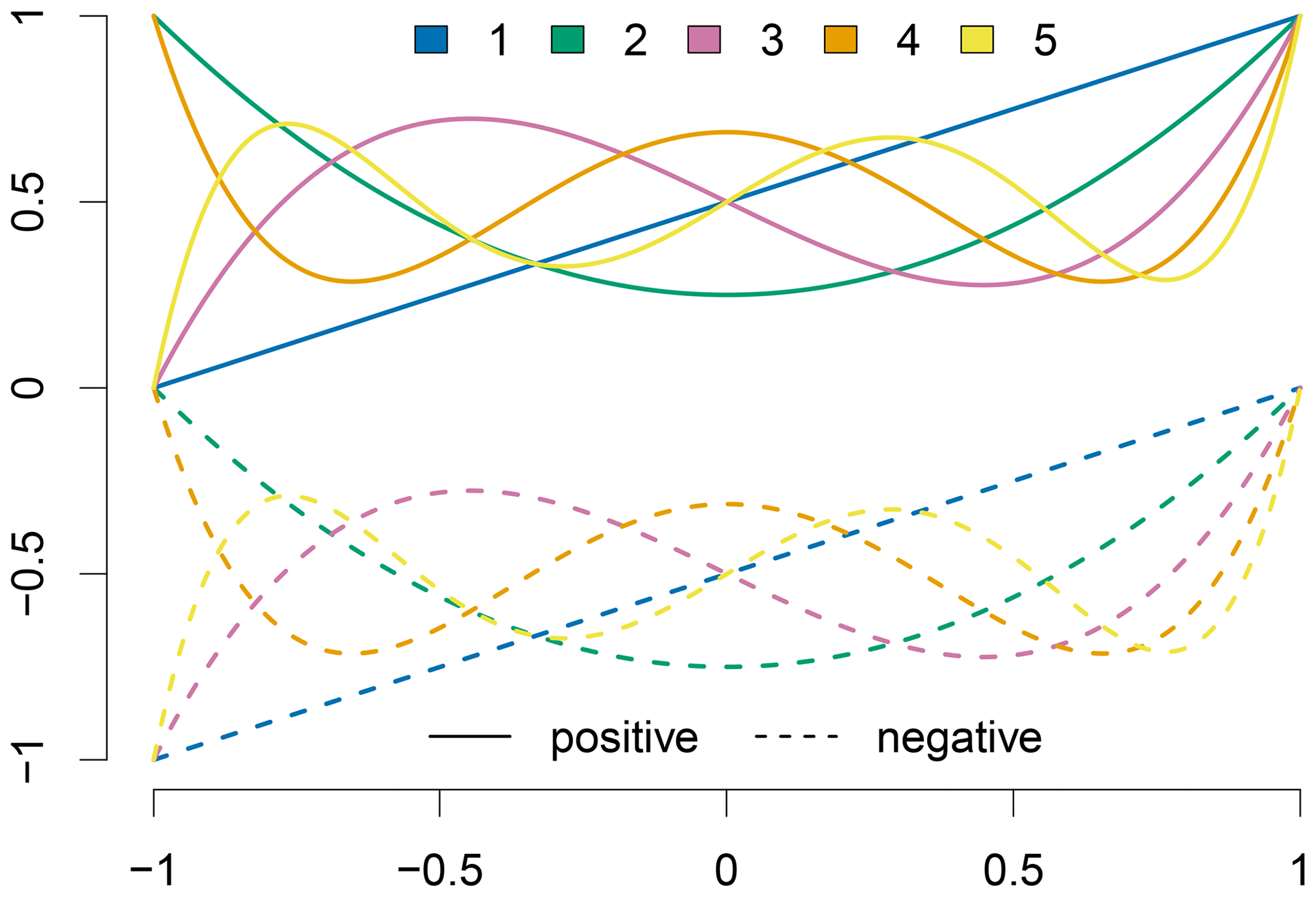
Figure 4Positively (solid) and negatively (dashed) transformed Legendre polynomials of order 1 to 5.
Thus, the interactions with the harmonic functions for the location parameter μ can be expressed as
These terms show the desired behavior as depicted exemplarily in Fig. 3 on the right-hand side.
Combining the seasonal and interannual variations with these interactions leads to a flexible model for the location parameter:
Using a VGLM, we allow the scale σ and shape ξ to vary in the same way. In many publications (e.g., Golroudbary et al., 2016; Rust et al., 2009) the shape parameter is described merely with a constant offset ξ0 to be estimated or is even set to a fixed value. The reason is that this parameter is regarded as difficult to estimate as it describes the behavior of the most extreme and thus very rare events. Papalexiou and Koutsoyiannis (2013) state that “the record length strongly affects the estimate of the GEV shape parameter and long records are needed for reliable estimates”. We assume our dataset will be sufficiently long. Fischer et al. (2019) have shown by means of an example station in Germany that a pronounced seasonal cycle in ξ exists with lower, partly negative, values in winter and higher values in summer. Those differences could be explained with the predominance of less intense stratiform precipitation in the winter months and more intense convective precipitation in the summer months. The performance gain of a seasonal–interannual shape parameter will be discussed in detail in Sect. 6.
3.5 Return levels
The p quantile of the GEV gives the return level rp for a certain non-exceedance probability p (or occurrence probability 1−p) and can be written as
Instead of stating the non-exceedance probabilities it is common to consider the respective average return period . The interpretation is that the return level is exceeded on average once in this particular time period. Since we consider return levels changing in time, the concept of a temporal change of a return period might be difficult to capture. Thus, in the following we refer to a (time-dependent) non-exceedance probability p(t) and the return period T(t) simultaneously. As we consider monthly maxima we calculate monthly return levels as well. Similar to, e.g., 100-year return levels obtained with annual maxima, we determine the 100-January return levels, the 100-February return levels and so on. In the following we state them as monthly 100-year return levels instead of naming respective months. This should not be confused with annual return levels. However, they can be calculated as well with monthly maxima, leading to more accurate and reliable annual results (Maraun et al., 2009; Fischer et al., 2018).
4.1 Stepwise model selection
After introducing the model setup in the previous section, the maximum orders for harmonic functions and Legendre polynomials have to be selected. Here, we set maximum orders H and I to five to ensure a feasible model selection procedure. The result of the model selection, which is described below, confirms that no order higher than 5 is required to adequately describe the data. With the full model consist of 348 coefficients (116 for each GEV parameter: 1 constant offset, 10 for seasonal variations, 5 for interannual variations and 100 interaction terms) for each station separately. This model is reduced to the necessary complexity with stepwise model selection using the Bayesian information criterion (BIC) (e.g., Neath and Cavanaugh, 2012). The procedure has two parts: first, only the direct effects are selected; in the second part, the interactions are added subsequently. Starting point is the stationary GEV (Eq. 2). In each iteration, every possible covariate is added once to the reference (in the first iteration: stationary GEV) and the BIC is determined. For the first iteration of part one this leads to 45 different models (15 for each GEV parameter). The model with the lowest BIC is selected as the best candidate for the next step. If the difference (as suggested by Fabozzi et al., 2014), the model is considered superior to the reference and becomes the new reference for the next iteration. Again, all remaining covariates are probed once for model improvement (leading to 44 different models for iteration two of part one), and the stepwise model selection is continued. If ΔBIC < 2 for all probed covariates, the current reference model is taken as the final model.
Now, the procedure is repeated for interaction terms starting with the final model from part one. To answer RQ1 (Sect. 5), in which we analyze the gain of including interannual variations, we also select for each station a seasonal-only model without interannual variability as a reference model. To address RQ2, model selection with different setups is used; details are given in Sect. 6.
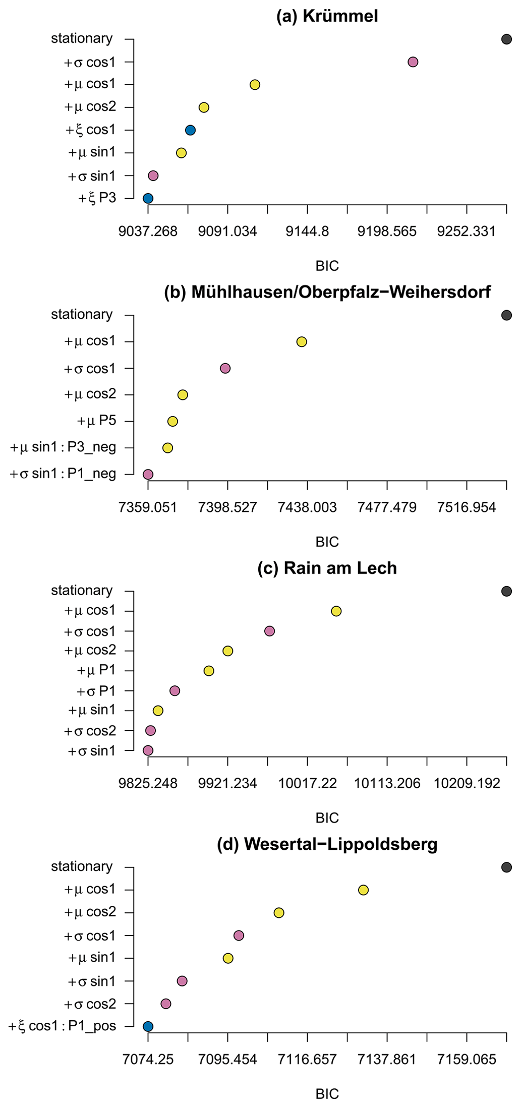
Figure 5Stepwise model selection for example stations. BIC against stepwise-selected covariates for location (yellow), scale (pink) and shape (blue) for each iteration. All covariates listed are included in the final model.
Figure 5 illustrates the stepwise selection for the four example stations. The BIC (x axis) decreases when adding necessary covariates (y axis from top to bottom). All covariates listed in the panels (Fig. 5) for the corresponding parameter (color) are included in the final model. Numbers following sin, cos and P indicate the respective harmonic/polynomial order. Terms with a colon denote interactions. For all four example stations, interannual terms in addition to seasonal ones have been included following the procedure described above; however, the type of interannual variation differs for each station. On the one hand, stations Rain am Lech and Wesertal-Lippoldsberg are characterized by a linear change in parameters. These changes occur in the μ and σ parameters for the former station, while for the latter the seasonal cycle of ξ changes linearly with the years. On the other hand, the extreme precipitation of the stations Mühlhausen/Oberpfalz-Weihersdorf and Krümmel is described with higher-order Legendre polynomials.
The model selection procedure was applied for all 519 stations individually. About 65 % of the stations () prefer a model with an interannual component. Those gauge stations are roughly equally distributed in space, and no common characteristics (e.g., stations altitude or record length) are apparent compared to stations without an interannual component. All models of the 338 stations contain seasonal variations as well. The properties of the interannual variability of those models are depicted in Fig. 6: (a) indicates those GEV parameters which show an interannual component; (b) shows whether an interannual component is part of a direct effect and/or an interaction; (c) gives the counts and portions of the selected Legendre polynomials (x axis) for the GEV parameter (y axis) and kind of covariate (direct: top; interactions: bottom). We do not show the spatial distribution of the Legendre polynomials since no clear pattern can be detected.
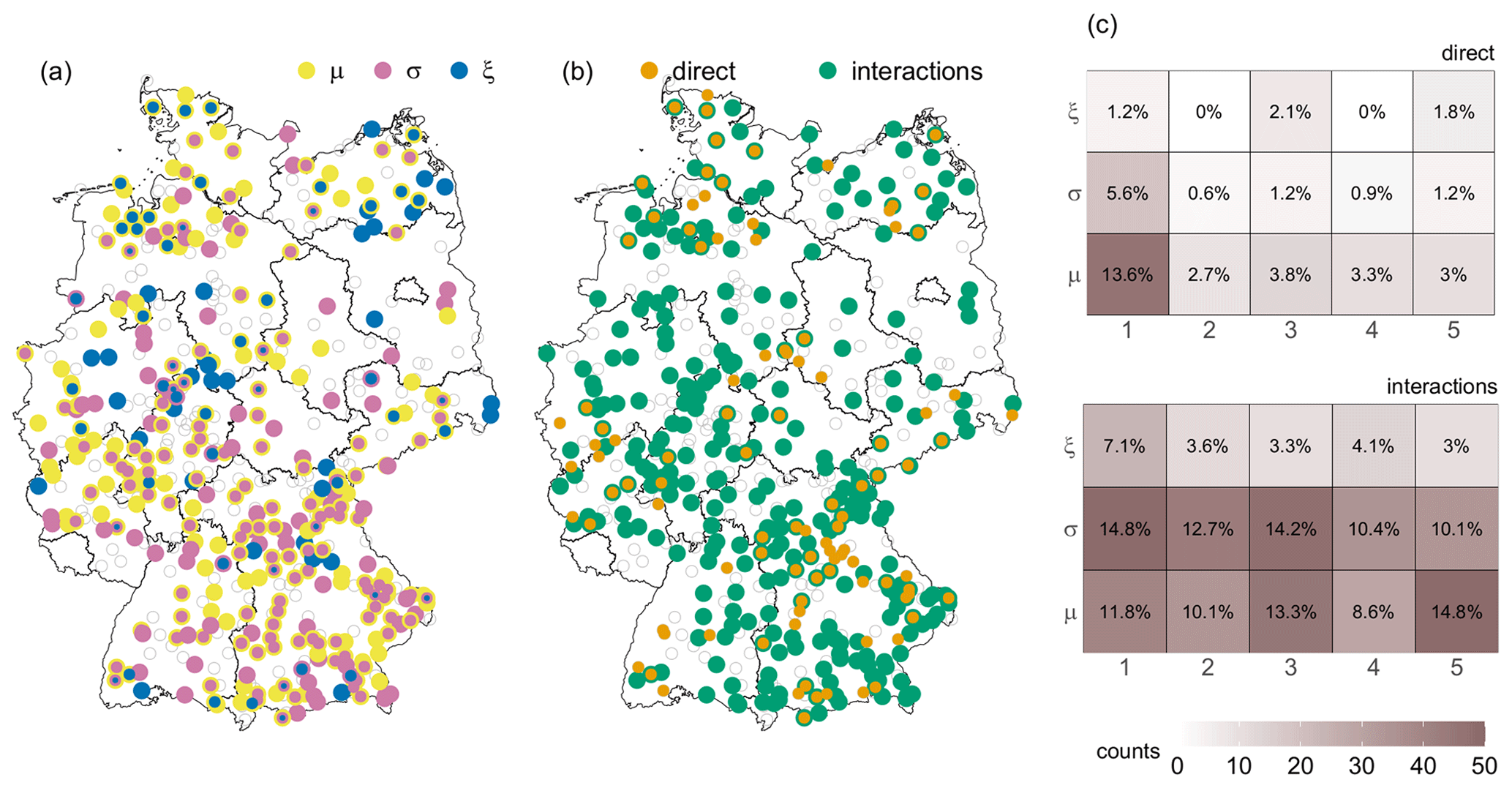
Figure 6Properties of the interannual variability components of those 338 models including at least one. (a) GEV parameter with interannual component, location (yellow), scale (pink) and shape (blue). (b) Direct (orange) and/or interactions (green) with interannual components. (c) Counts (color intensity) and portion (percentage) of selected orders of the Legendre polynomials (x axis) for different GEV parameters (y axis) divided for direct (top) and interactions (bottom) for the 338 models. Stations with no interannual component are marked as transparent circles.
It can be seen that the selected interannual covariates are partly very variable in space. This can be explained by (1) a large spatial variability in extreme precipitation due to partly small-scaled events and (2) the model selection procedure, which chooses one suitable model, even if other models are comparably appropriate. However, common characteristics can be detected. The GEV's location and scale parameter are mainly affected, and interannual changes in the seasonal cycle (interactions) dominate. Nevertheless, changes in the shape parameter and changes without affecting the seasonal behavior occur, often for several stations of the same region, indicating common local characteristics. The stations with direct effects are mainly characterized by a linear interannual change in the location parameter. For the interactions, the preferred Legendre polynomial is not so obvious.
4.2 Model verification tools
To answer RQ1 and RQ2 the performance of a model with respect to a reference has to be analyzed. We use the quantile skill score (QSS) (Bentzien and Friederichs, 2014; Friederichs and Hense, 2007), which is based on the quantile score (QS) defined as
Here ρp denotes the check function, defined as
with . The QS is a weighted mean of differences between the N observations on and the quantiles (return levels) rp,n for a certain non-exceedance probability p. It is positively oriented and optimal at zero. We use leave-one-year-out cross validation to obtain a robust quantile score estimate.
The quantile skill score (QSS) is defined as
with the perfect score QSperf=0. For a model outperforming the reference, the QSS is in the range (0,1], giving the fraction of improvement with respect to the difference between the perfect and the reference model; for models worse than the reference, QSS < 0.
For stratifying verification along months or stations we use the decomposition of the QSS (Richling et al., 2024) to learn about peculiarities of certain subset,
with K being the number of different subsets; e.g., for monthly stratification K=12. The quantile skill score for the full dataset can be decomposed into the sum of a weighted quantile skill score for the different subsets. The term in Eq. (18) represents the subset QSS, weighted, on the one hand, with the so-called frequency weighting , indicating how many data points can be attributed to that subset, and, on the other hand, with the reference weighting , indicating how well the reference can represent the data for the given subsets with respect to the complete dataset. The weighted subset QSS can be regarded as the contributions to the total QSS.
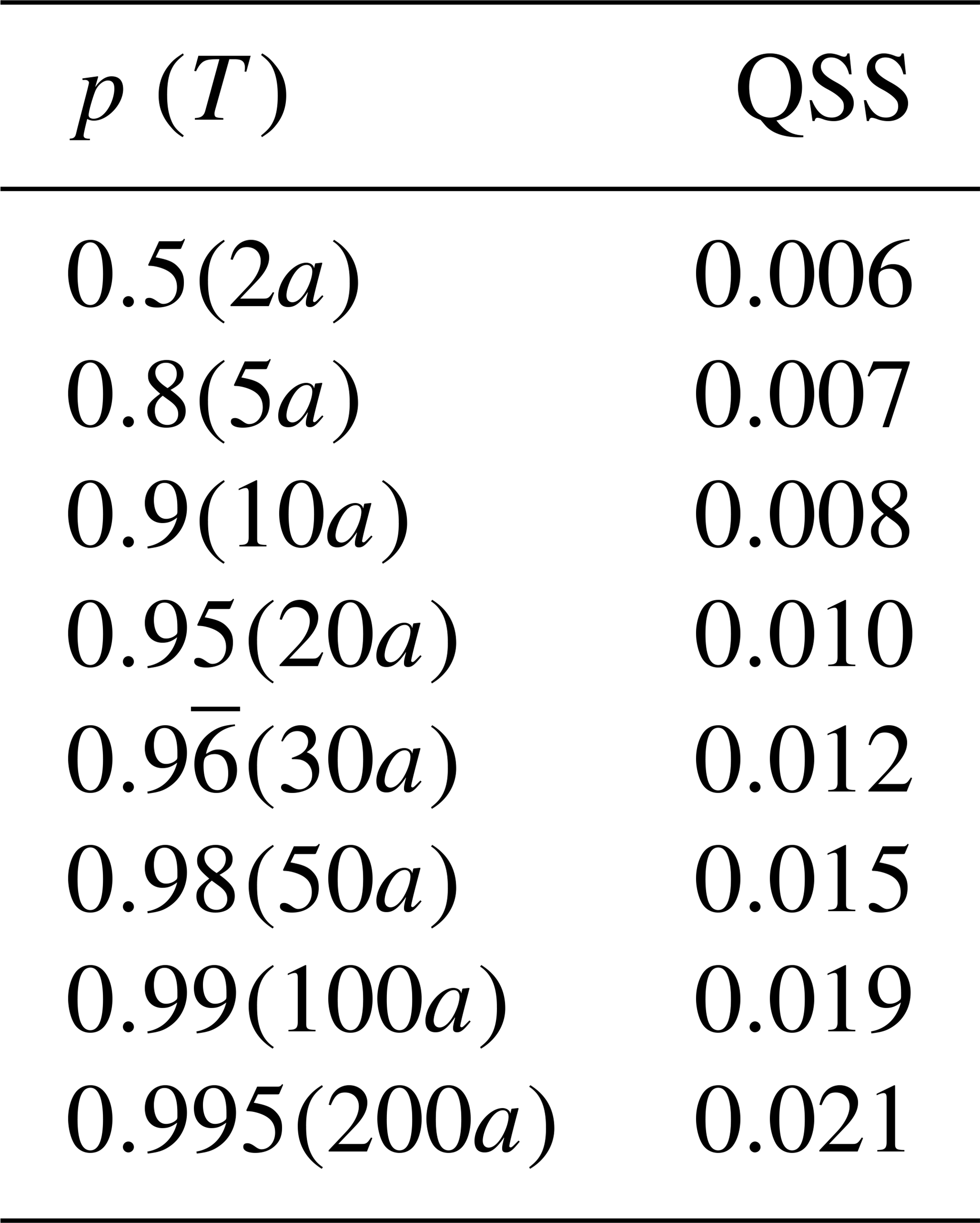
We address RQ1: can a model with interannual variations better represent the observations than a seasonal-only model? As mentioned in Sect. 4.1, a model with at least one interannual component in any of the GEV parameter was chosen only for 338 of 519 stations (∼ 65 %). To assess the importance of the interannual variations of these 338 stations, we analyze the skill with respect to the seasonal-only model. Table 1 shows the total QSS for different non-exceedance probabilities (return periods). Skill is positive but small ≲ 2 %, increasing with non-exceedance probability (return period). The latter has to be interpreted with care as there are very few observations in the range of the upper quantiles. Return levels with a return period higher than the time range of the data should be treated cautiously, since the quantile score cannot reasonably evaluate those values (Fauer and Rust, 2023). As we consider for each station at least 80 years of observations, this only matters for non-exceedance probabilities (return periods) of 0.99 and 0.995 (100 and 200 years). The small increase in skill due to the inclusion of interannual variation is expected as most of the signal can be described already with the strong seasonal cycle.
Table 1Total QSS for different non-exceedance probabilities p (return periods T) of the seasonal–interannual model with respect to the seasonal-only model averaged over 338 stations with an interannually varying component.
We analyze whether interannual variations improve the estimates of return levels for a particular month and stratify the QSS along months, Fig. 7a. To understand the importance of the monthly subset scores, the reference weighting (Fig. 7b) and the contribution to the total skill score (Fig. 7c) are shown. The frequency weighting is (almost) identical for all subsets (as the records generally contain complete years) and is not shown. Averaged over all 338 stations, the monthly QSS (Fig. 7a) is positive for all months, and non-exceedance probabilities for spring (March, April) and summer (July, August) stand out. For the contribution to the total QSS, the reference weighting (Fig. 7b) gives more importance to the summer months, leading to the strongest contribution to total QSS in July. The structure of the reference weighting term (Fig. 7b) indicates that the seasonal-only model does not represent the observations in summer as well as in winter. This probably indicates a stronger need for taking interannually varying return levels in summer into account. Adding the values of Fig. 7c by row leads to the values depicted in Table 1. The monthly QSS averaged over 338 stations leads to a consistently positive skill, but the performance varies strongly for the different stations.
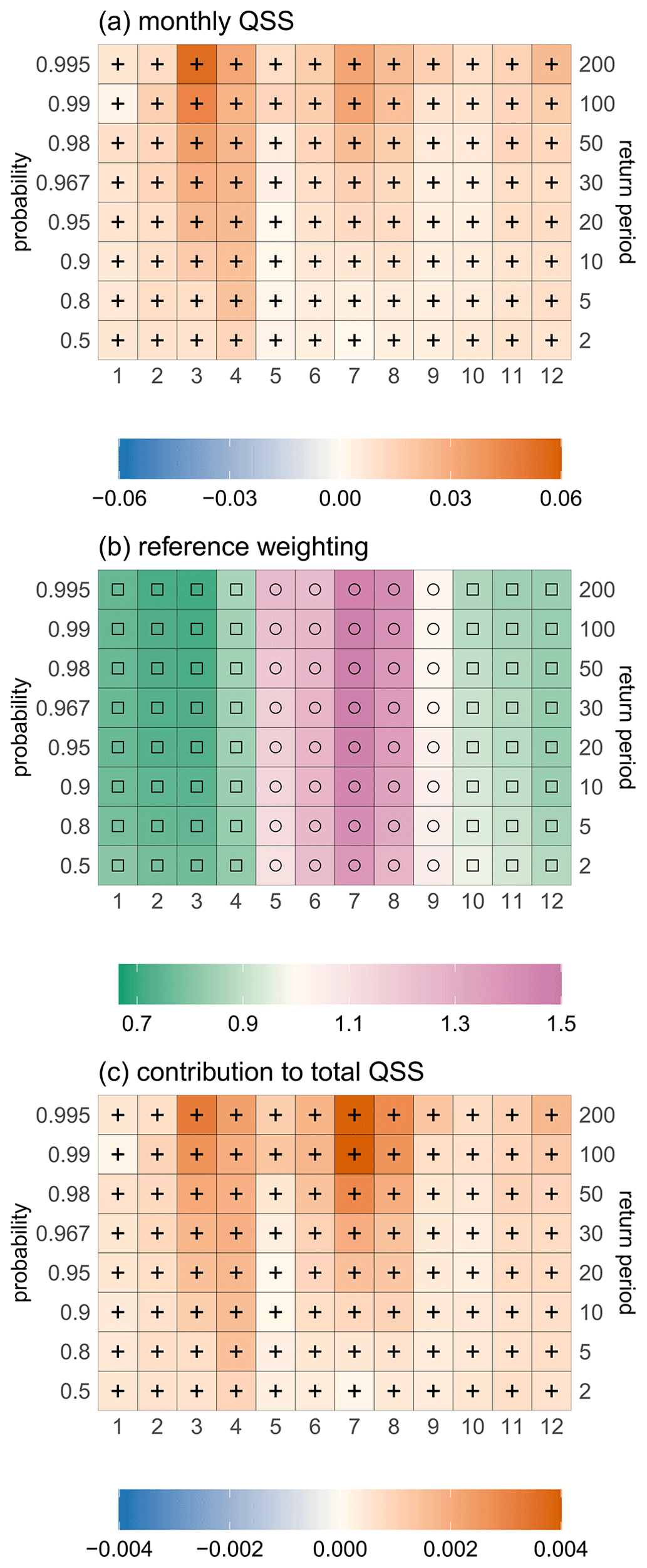
Figure 7Subset QSS (a), reference weighting (b) and the contribution to the total QSS (weighted subset QSS) (c) for the months of January to December (x axis) averaged over 338 stations with interannual components for different non-exceedance probabilities (left y axis)/return periods (right y axis). Positive/negative values (orange; plus sign/blue; minus sign) of the QSS (weighted QSS) indicate an increased/decreased performance of the seasonal–interannual model with respect to the seasonal-only model. The reference weighting describes how well the seasonal-only model describes the subset data with respect to the full dataset: green (squares)/pink marks (circles) a better/worse representation.
We now stratify verification also along stations (K=338) and average over all time steps. The subset QSS for the non-exceedance probabilities of are plotted in Fig. 8, and the reference weighting is exemplarily illustrated for p=0.99 (since the patterns are similar for all non-exceedance probabilities) in Fig. 9. The frequency weighting and the contribution to the total QSS are not shown, since the first one does not exhibit any spatial pattern and the last one does not visually distinguish from the figure of the subset QSS. For most of the stations the seasonal–interannual model can represent the observations better than the seasonal-only model.
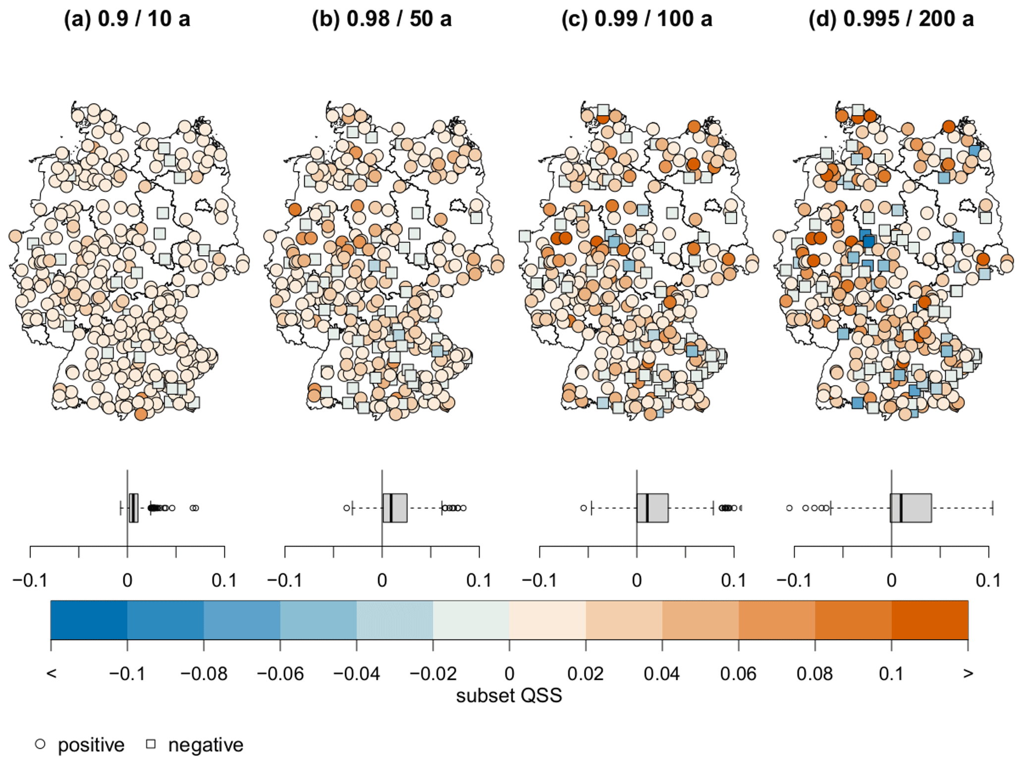
Figure 8Subset QSS for 338 different stations for the non-exceedance probability/return period of (a) 0.9/10 years, (b) 0.98/50 years, (c) 0.99/100 years and (d) 0.995/200 years. The distribution of the subset QSS is depicted as a box–whisker plot and in space (map). Positive/negative (orange circles/blue squares) values mark a gain/loss in skill.
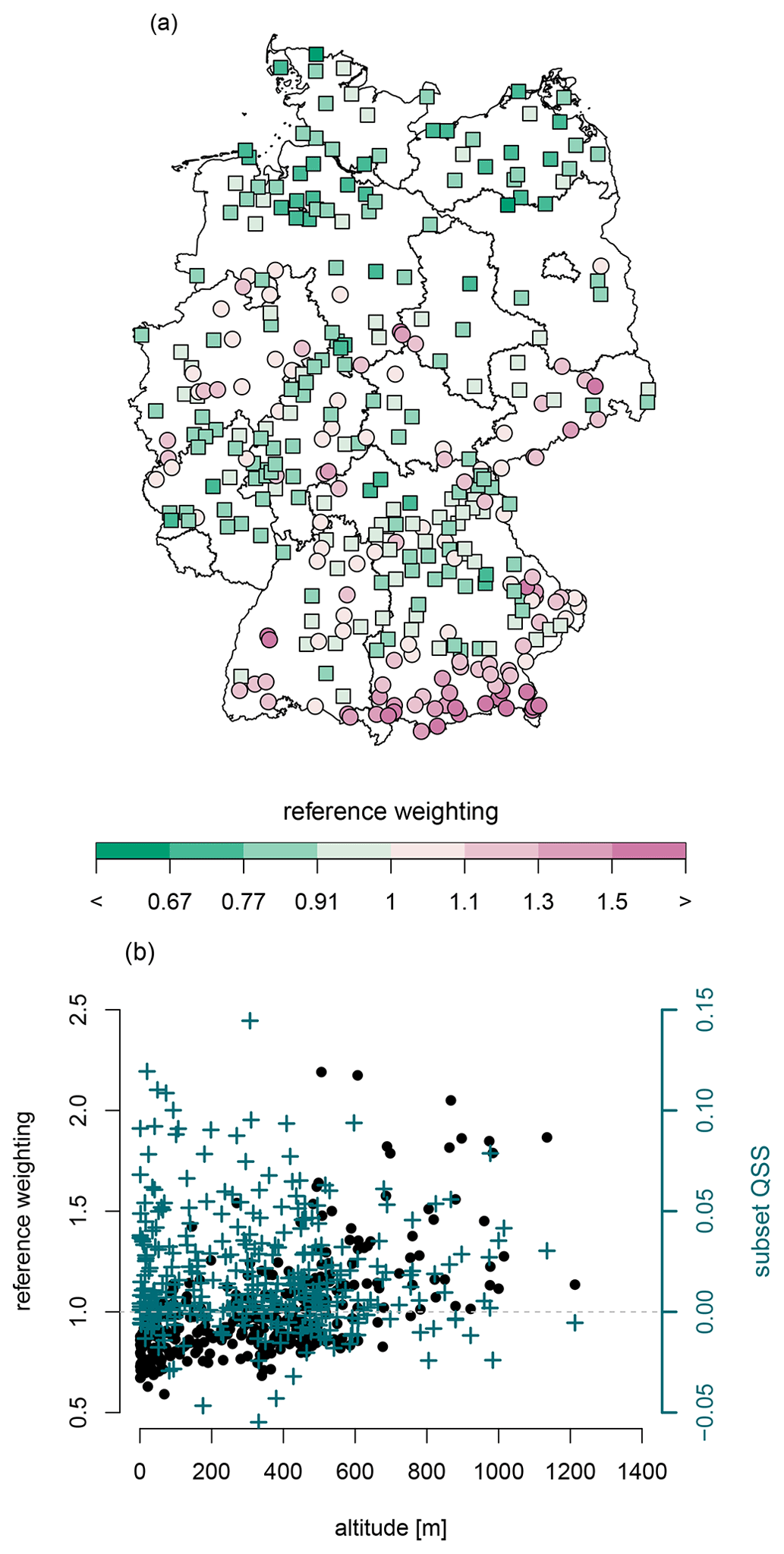
Figure 9Map of reference weighting for non-exceedance probability 0.99/return period 100 years (a). Green/violet values refer to a better/worse representation of the data by the reference (seasonal-only model). The reference weighting of other non-exceedance probabilities is barely different. Reference weighting plotted against station altitude (b, black dots) indicates better performance for the reference in the lowlands than in mountainous regions. The subset QSS (second axis, blue crosses) of the seasonal–interannual model does not show an improved skill for stations at higher altitude.
Only for a few records and higher non-exceedance probabilities/return periods do the variations with the years lead to more uncertain return levels, for example station Wesertal-Lippoldsberg. The monthly contribution to the QSS for this station is depicted in Fig. 10b. The negative skill mainly arises from overestimated return levels for the summer months, especially for the recent years (visually verified in Sect. 7). This merely occurs for higher return periods due to the interannually varying shape parameter ξ (see Fig. 6). However, a worse skill for stations with an interannual component in ξ cannot be detected in general (not shown). We discuss the change in the seasonal cycle of Wesertal-Lippoldsberg in more detail in Sect. 7.
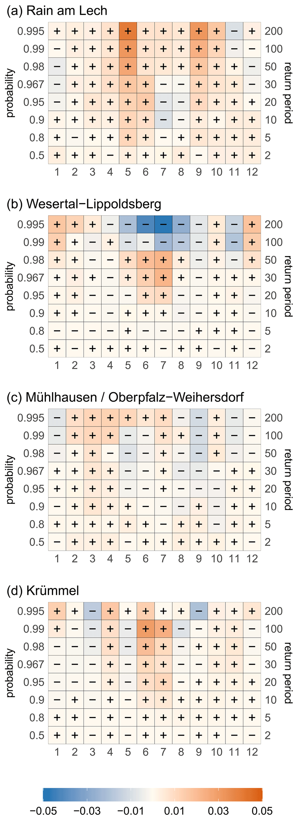
Figure 10Monthly contribution (x axis) to the station-wise QSS depicted in Fig. 8a for the example stations shown for different non-exceedance probabilities (left y axis)/return levels (right y axis). Positive/negative values (orange/blue) indicate a gain/loss in skill of the seasonal–temporal model with respect to the only seasonal model.
Compared with the location heights of Fig. 1, the reference weighting for the station-wise analysis in Fig. 9 shows a clear relationship to station altitude and specifies that the seasonal-only model cannot reflect the data in mountainous regions as well as in lowlands. Analyzing the skill of the seasonal–interannual model with respect to the altitude does not show an improvement, especially for higher located stations (b, blue crosses). This might indicate that both model setups miss important mechanisms for extreme precipitation in mountainous regions (e.g., convection due to lifting or flow direction). Thus, these processes cannot be approximated by solely including temporal covariates but need to be modeled directly and/or via appropriate spatial covariates. This weak point cannot be seen for the example stations, since they are located in the lowlands (Krümmel: 64 m; Wesertal-Lippoldsberg: 176 m) or in the low mountain ranges (Rain am Lech: 409 m; Mühlhausen/Oberpfalz-Weihersdorf: 420 m).
Besides the monthly contribution to the station-wise skill for Wesertal-Lippoldsberg, Fig. 10 also shows the results for the other three example stations. Rain am Lech serves as an example with a very high skill mainly dominated by a better reflection of the data for the months of May and September. At Mühlhausen/Oberpfalz-Weihersdorf the return levels for spring can be estimated slightly better than for autumn, and Krümmel is dominated by a positive skill for June and July.
In summary, it can be noted that modeling interannual variations is beneficial for estimating return levels for all months, especially for the summer season. However, at a few stations the flexible modeling leads to a partly worse representation, in particular for larger return periods. Both seasonal modeling and seasonal–interannual modeling may have difficulties capturing mechanisms for precipitation formation in alpine regions.
Analyzing the selected models of the 519 considered stations shows that about 34 % ( stations) prefer a model with interannual and/or seasonal variations in ξ. Figure 11 illustrates the spatial occurrence and the kind of variation (seasonal, interannual or interaction). It is noticeable that the density of stations with a flexible ξ is much higher in the north and east of Germany than in the south. The reason for a location-dependent variable shape parameter is an interesting question for further studies. We assume that different meteorological processes play a major role, e.g., the influence of weather types or the kind of precipitation (stratiform or convective). A dependence of flexibility in ξ on the record length is not obvious (not shown). Most of the stations (, about 60 %) are represented by a model including seasonal variations, whereby many of them ( stations) do not favor an interannually varying shape parameter at all. Only a few stations (, about 10 %) prefer a model with direct interannual changes. Nevertheless, two regions with a slight agglomeration of direct interannual changes can be detected: in the middle of Bavaria (federal state in the southeast) and in the northeast around the Mecklenburger Seenplatte (also known as Mecklenburg Lake Plateau) represented by the example station Krümmel. About 39 % of the stations () show an interannually varying seasonal cycle (interactions); these stations are almost uniformly distributed across Germany, with a somewhat higher density around the example station Wesertal-Lippoldsberg.
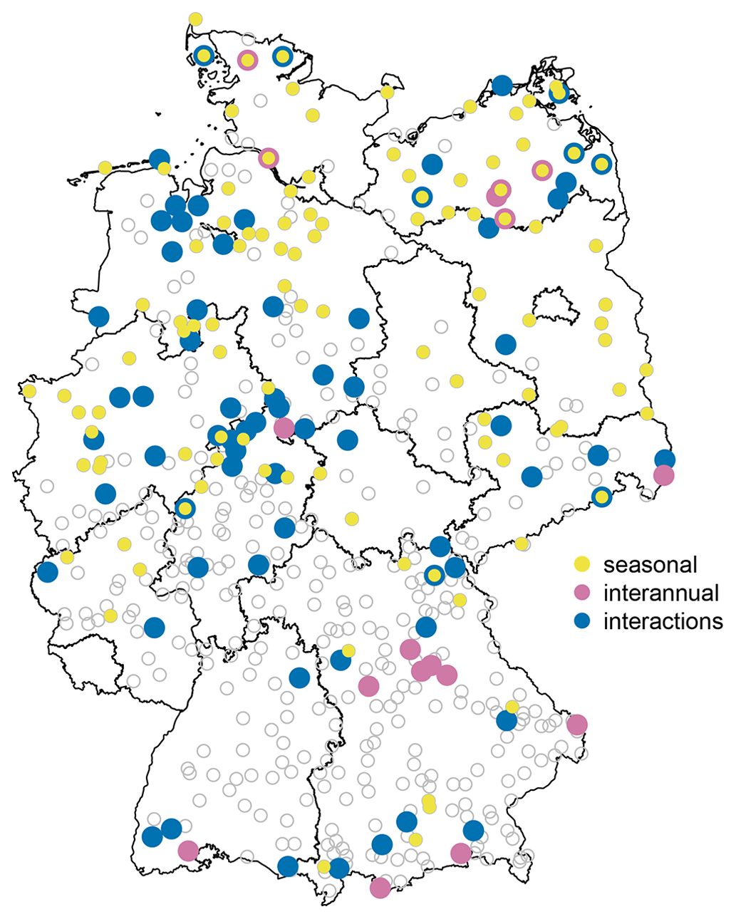
Figure 11Spatial distribution of stations with flexible shape parameter ξ. Seasonal variations (yellow) occur at stations, interannual (pink) at stations and interactions (blue) at stations. Gray circles mark the stations without variations in ξ.
We (a) quantify the gain from a flexible shape parameter with respect to a model with constant ξ and (b) analyze the contributions of the seasonal, interannual and interacting variations. To this end we use four model selection setups with a focus on ξ: setup (1) with constant ξ; setup (2) with seasonal components in ξ; setup (3) with seasonal and interannual components in ξ; and setup (4) with seasonal and interannual components, as well as their interactions in ξ. All other parameters are allowed to have seasonal, interannual and interacting components in all setups. Figure 12 illustrates the gain in performance for the different steps. The monthly skill for seasonal–interannual variations including interactions against a constant ξ averaged over the 178 stations expressed as the contribution to the total QSS is depicted in the top panel. There is positive skill for all months and return periods (with some exceptions with slightly negative values). The highest contribution to the total skill arises from the summer months, for which the reference weighting is increased (Sect. 5).
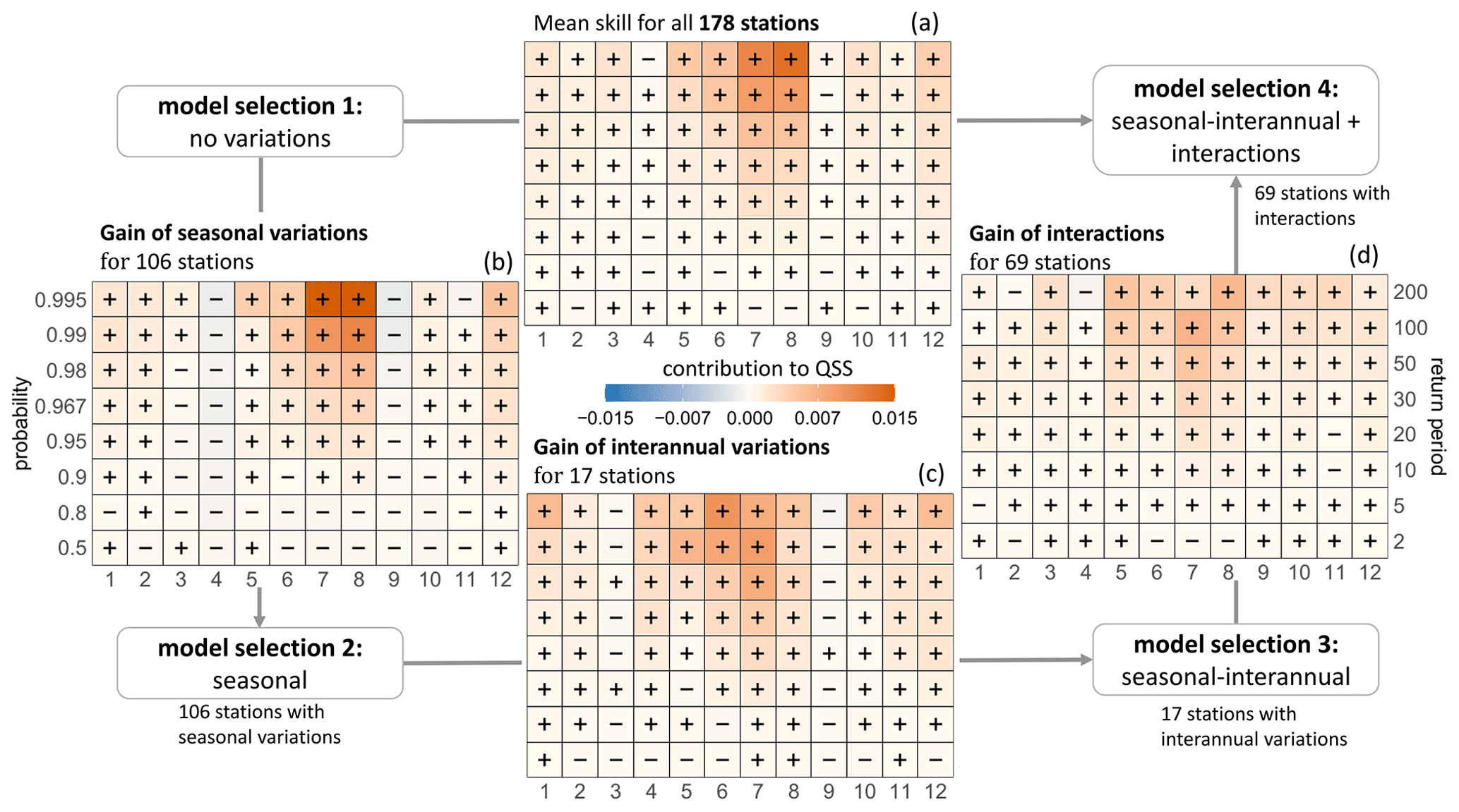
Figure 12Scheme for analyzing the importance of and performance gain by a flexible shape parameter as contribution to the total QSS. Illustrations (axes, colors, signs) equal to Fig. 10. The gain of adding seasonal variations in ξ (left plot) is analyzed for 106 stations as a result of a model selection with only seasonal components in ξ (setup 2). A model selection with constant ξ (setup 1) is used as reference. The bottom panel shows the gain of seasonal and interannual components (17 stations, setup 3) with respect to a seasonal-only ξ (setup 2). The right panel finally show the gain by allowing interactions (setup 4) with respect to setup 3 (without interactions) for 69 stations. The skill of a flexible shape parameter (seasonal, interannual and interactions) with respect to a constant ξ is shown in the top panel for 178 stations.
To analyze the contribution of the seasonal component to the skill, we use setup 2 (seasonal-only in ξ) against a constant ξ (setup 1). Setup 2 results in a variable shape parameter for 106 of 178 stations; for the rest of the records a model with no variations in ξ was preferred. The skill of these 106 stations with respect to setup 1 is depicted in the left panel of Fig. 12. Seasonal flexibility in ξ improves in particular the return levels for summer; there is a very small gain in winter. For the transitional months March/April and September the increased flexibility led to a slightly worse model. A change in the shape parameter could indicate a change in the dominating precipitation type (convective in summer, stratiform in winter). The flexible modeling does not benefit months characterized by the transition of the precipitation regime, since no dominating precipitation type exists. A variable ξ for the season mainly improves the return levels of the higher return periods, while the skill for 2 and 5 years is slightly decreased.
Setup 3 evaluates the gain by adding an interannual component to ξ with respect to a seasonal-only model (setup 2). Only 17 stations preferred this type of model, but for those we found an improvement of the return level estimates for all months (bottom panel). The interannual variations do not improve the performance for the transitional months of March and September. Additionally, the lower return periods of 2 and 5 years do not benefit from this flexibility.
In setup 4 we allow additionally for interactions and compare the selected models with those chosen in setup 3 (seasonal–interannual model without interactions). The skill averaged over 69 stations with interaction terms for ξ is shown in the right plot of Fig. 12. The interactions improve the return levels for all months and return periods, especially for the summer months, and are able to faintly compensate for the lack of skill for the lower return periods and the transitional months. The skill shown in Fig. 12 is averaged over the respective stations; however, the performance for the individual stations can differ. For example, as already mentioned in Sect. 5 and analyzed in more detail in Sect. 7, the 100-year and 200-year return levels at the example station Wesertal-Lippoldsberg are overestimated (visually obtained by comparing return levels and observations) for the last decades, resulting in a worse representation of the most recent data. The overestimated return levels can be explained by considering the seasonal cycle of the shape parameter ξ for different years (1931, 1976, 2021) in Fig. 13. As depicted in Fig. 5 the shape parameter at this station can be expressed with (according to Eq. 13), i.e., a linear rise in the amplitude. Thus, for the first observational year 1931 the amplitude is modeled to be zero and increases linearly with time, reaching its maximum for the last year in the record (2021). While for earlier years this linear change represents the extreme precipitation quite well, for the end of the record the values of ξ, especially for summer, become very large, which cannot be supported by the sparse database.
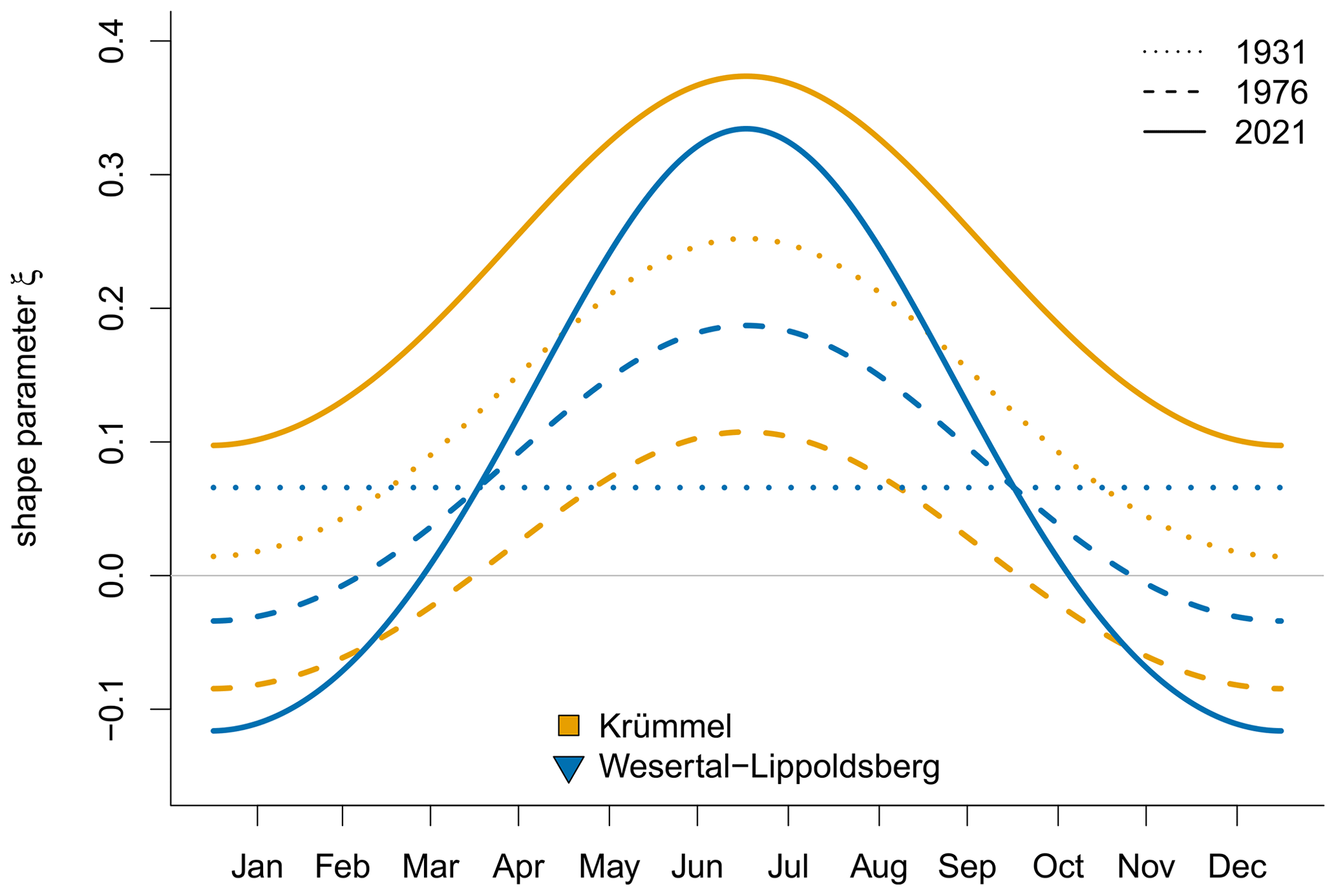
Figure 13Seasonal cycle of the shape parameter ξ for the example stations Krümmel (orange) and Wesertal-Lippoldsberg (blue) for the years 1931 (dotted), 1976 (dashed) and 2021 (solid). The station symbols in the legend are selected according to the station positions of Fig. 1.
Additionally, Fig. 13 shows the seasonal cycle in ξ for the example station Krümmel, whose shape parameter is composed of . Seasonality remains unchanged while the direct effect of the third Legendre polynomial leads to a shift of the cycle to smaller/larger values of ξ in 1976/2021 compared to 1931, leading to pronounced variability in the return levels of this station. The seasonal cycles for the example stations will be discussed in more detail in Sect. 7.
A negative shape parameter is unusual for describing the GEV distribution of extreme precipitation (Papalexiou and Koutsoyiannis, 2013; Ragulina and Reitan, 2017) since the resulting distribution is characterized by an unnatural upper bound. In our analysis the shape parameter is able to change with time such that negative values for ξ for a certain period are considered to be unproblematic.
In general, a varying shape parameter leads to a better representation of the data for all months and return periods, in particular for the very extreme events in summer; the flexibility leads to a worse skill of return level estimates only for very few stations.
In this section we aim to assess the impact of climate change on seasonal extreme precipitation (RQ3). With a simple linear model for each month and station, we quantify the interannual variation of return levels for a given non-exceedance probability. We compare the time period from 1941 to 2021 where all stations have data. Note that estimating linear trends for fixed (and short) periods of time can yield very different results, depending on the considered time period due to decadal variability. Thus, the trend estimates presented here for the given time period serve as a rough indicator for climate change effects; for a more detailed analysis, all the datasets should be taken into account for each station. Appendix A explains the calculation of the linear trend in more detail. Figure 14 illustrates the proportion of stations with a positive, negative or no trend for (a) the 2-year, (b) 10-year and (c) 100-year return levels. The trends are stated in relative changes from 1941 to 2021. Changes are mainly very weak (< 5 %); only 15 % to 35 % (depending on the month and occurrence probability) show more pronounced trends. In general, an increase in the return levels occurs more often than a decrease for all return periods, especially in June (more than 3 times more often). A decline slightly prevails only for the return levels in April. The patterns of the 5- to 200-year return levels are similar but with smaller trends for the shorter return periods. The characteristics of the 2-year return level differ: an increase is more often visible for the months of March and September to November with a less pronounced signal for the summer months. In contrast to that, the trends of the 100-year return level are stronger in summer.
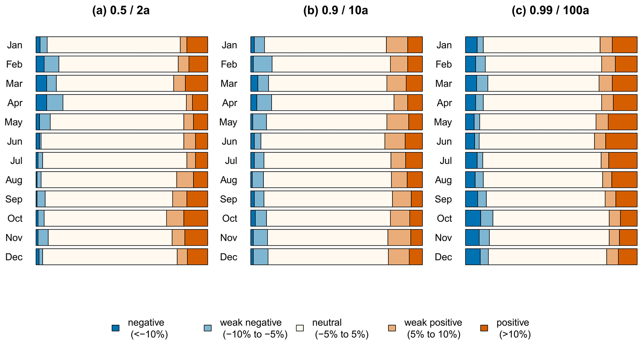
Figure 14Proportion of stations with a positive (light/dark orange), negative (light/dark blue) or neutral (white) relative change from 1941 to 2021 for the (a) 2-year return level (p=0.5), (b) 10-year return level (p=0.9) and (c) 100-year return level (p=0.99) for the months of January to December (rows).
About 35 % to 50 % of the considered 338 stations ( 2-year return level, 10-year return level, 100-year return level) show a change larger than 5% for at least 1 month of the year. The trends are regionally very different (maps for 2-year and 100-year return levels are given in Appendix B). Despite the partly very small-scaled characteristics, uniform behavior for several regions can be detected. Two of these regions with more pronounced changes are considered in more detail: one in southern Germany represented by the station Rain am Lech and the other one in the center of Germany exemplified by the station Wesertal-Lippoldsberg.
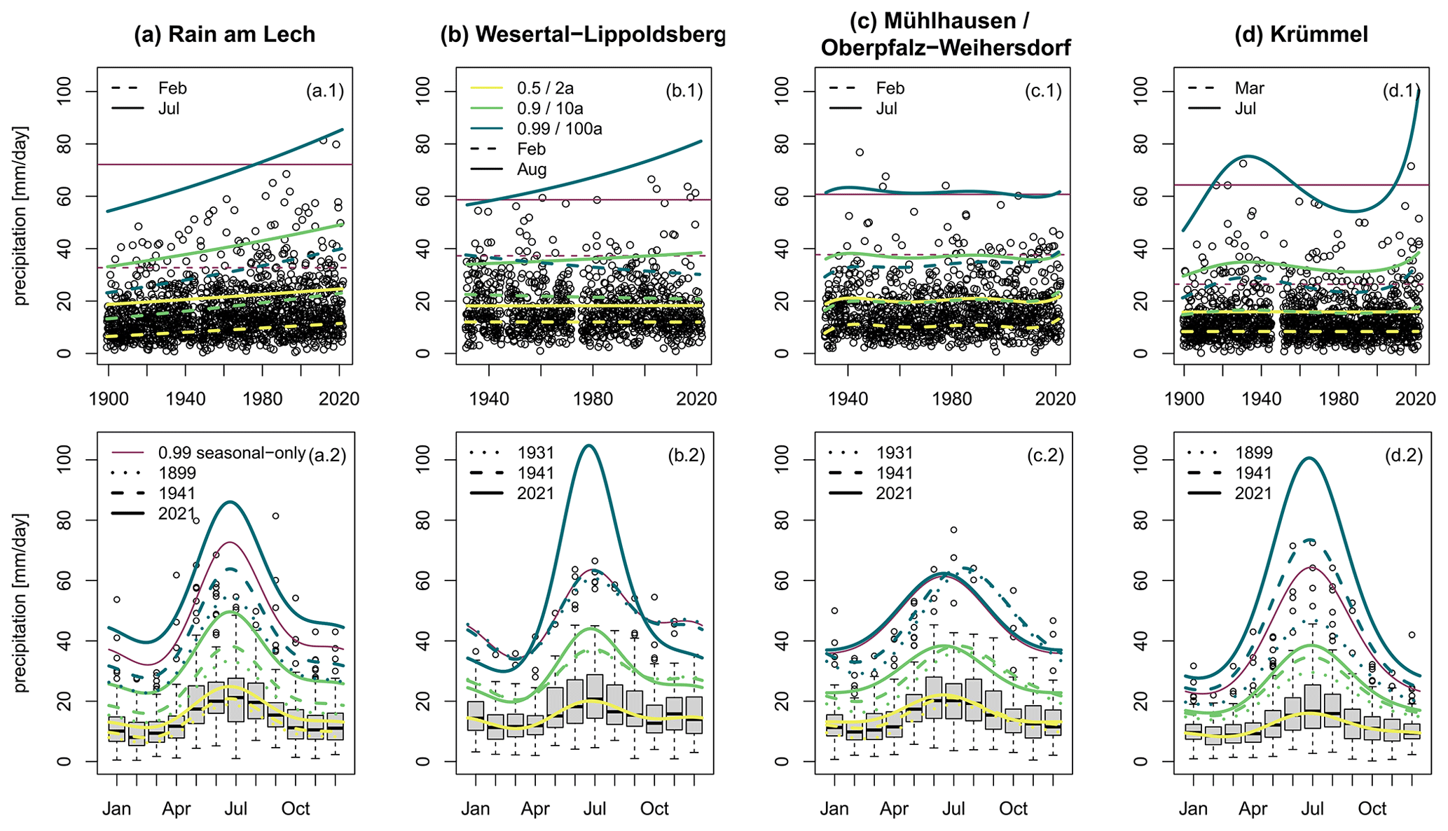
Figure 15Observations and return levels for the stations Rain am Lech (1 January 1899 until 31 December 2021) (a), Wesertal-Lippoldsberg (1 January 1931 until 31 December 2021) (b), Mühlhausen/Oberpfalz-Weihersdorf (1 January 1931 until 31 December 2021) (c) and Krümmel (1 January 1899 until 31 December 2021) (d). The top row shows the observations (dots) and the 2-year (yellow), 10-year (green) and 100-year return levels (blue) for the months with lowest/highest return level (dashed/solid) against time (years, x axis). Additionally, the 100-year return levels of the seasonal-only model are depicted for the same 2 months (burgundy). The bottom row depicts the seasonal cycle of the return levels for the first observation year (dotted), 1941 (dashed), and 2021 (solid) and the observations as box–whisker plots. Additionally, the 100-year return levels of the seasonal-only model (burgundy) are depicted in both rows as well.
The 2-, 10-, and 100-year return levels for the station Rain am Lech are depicted in Fig. 15a. Besides the interannual changes (a.1), the seasonal cycle for the first/last record year (1899/2021) and the first year of the common time period (1941) is shown (a.2). The return levels of this region are characterized by an increase for all months and return periods. For instance, the largest 100-year return level in the year occurring in summer rose from 54.6 mm d−1 in 1899 to 86.0 mm d−1 in 2021, corresponding to an increase of about 58 %. Considering the 100-year return levels of the seasonal-only model demonstrates that a non-interannual approach leads to highly underestimated values, especially for the first record decades. The model selection reveals that not only the location parameter changes linearly with the years but also the scale parameter (Fig. 5). The model verification (Fig. 10) confirms that the trend in the return levels is necessary for an adequate description of the observations, especially for the transitional months of May, September and October. Thus, an increase in extreme precipitation amounts as expected from the anthropogenic climate change can be seen very clearly for this region.
The second region, which is considered in more detail, is characterized by a decrease in return levels in winter and an increase in summer, leading to a rise of the seasonal cycle's amplitude. Figure 15b shows the 2-, 10-, and 100-year return levels for the station Wesertal-Lippoldsberg. Since the interannual change for this station is best described by a model with a flexible shape parameter only (Fig. 5), the 2-year return levels remain constant with the years. Towards higher return periods, changes are more prominent. They are pronounced for summer and winter, while the transitional months of March/April and September/October remain unaltered. The change in the seasonal cycle could be attributed to a combination of different processes. On the one hand, a higher water content of the air due to a temperature rise leads to an increased potential for extreme precipitation, particularly pronounced in summer. On the other hand, climate change can affect the characteristics of weather types and large-scale atmospheric circulations (e.g., NAO), which could result in a change in extreme precipitation as well in winter. The model verification (Fig. 10) confirms that a model with a changing seasonal cycle better represents the data observed in summer for return periods of 10 to 50 years, while the 100- and 200-year return levels are strongly overestimated with respect to the observations, especially for the most recent decades. In contrast, the seasonal–interannual model is more beneficial for estimating winterly return levels with return periods longer than 30 years. These characteristics can be seen as well by comparing the 100-year return levels of the seasonal–interannual model with those of the seasonal-only model.
In addition to a change in the precipitation's magnitude, a phase shift can influence the risk of damage as well. Therefore, we also analyze the linear change in the phase expressed as the day in the year with the highest return level for the time period 1941–2021. Here, a simple linear model is adequate for the cyclic variable since a shift of the day with the highest precipitation from December to January or vise versa does not happen at all. The change of the phase in days for different return periods is illustrated in Fig. 16a. More than two-thirds of the stations show less pronounced changes (< 5 d). In general, a shift to earlier times in the year appears more frequently for almost all return periods except of the 2-year return level. For the latter, several different regions with strong shifts to later times and only one large contiguous area in the north with a shift to earlier times can be detected (Fig. 16b). For the 100-year return level (Fig. 16c), such distinct regions do not appear, but in general a shift to earlier times prevails for the whole country. The latter behavior can be appreciated in station Mühlhausen/Oberpfalz-Weihersdorf, whose 2-, 10- and 100-year return levels are depicted in Fig. 15c. The shift of the seasonal cycle to earlier times leads to increased return levels for the first half of the year, such that the 100-year return level in spring is about 13 mm d−1 higher in 2021 than it was in 1931. The decrease in autumn appears weaker, with a maximum change in the 100-year return level of about −8 mm d−1. During the 90 years of observations the annual maxima of the 100-year return level has shifted forward by 35 d. Since only a shift and not a rise of the seasonal cycle occurs, the analysis of annual maxima would not show any changes. In general, a shift of the seasonal cycle to earlier times leads to an increased risk potential. The probability of flooding events rises since snow melting and heavy precipitation coincide in spring. Additionally, higher crop losses may occur since plants are more vulnerable to extreme precipitation during early growing stages. Although differences between the 100-year return levels of the seasonal-only and the seasonal–interannual model are not very pronounced, the shift from late summer to early summer, which might be continued in the future, cannot be detected with the non-interannual approach.
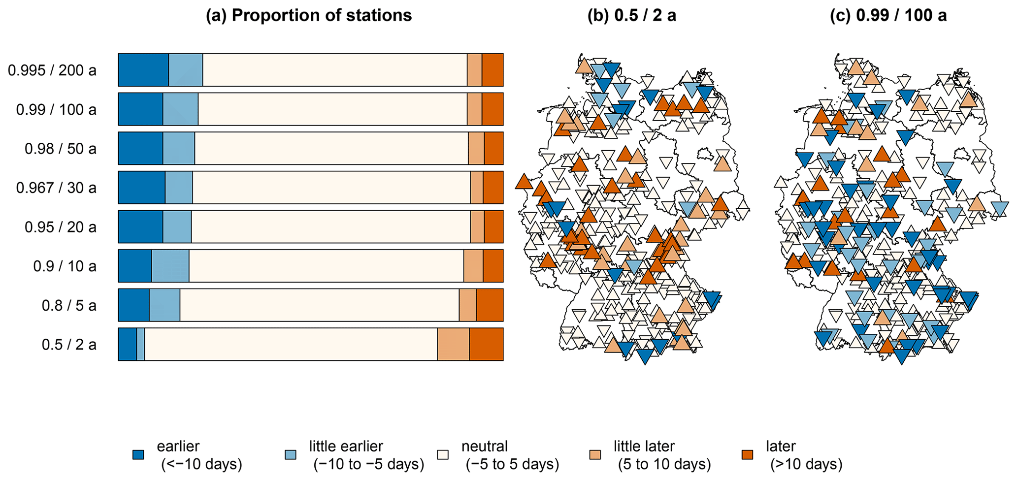
Figure 16Phase shift in days from 1941 to 2021 for the non-exceedance probability/return period of (a) 0.5/2 years, (b) 0.8/5 years, (c) 0.9/10 years and (d) 0.99/100 years. A shift to later/earlier times is marked with triangles pointing up/triangles pointing down. Minor changes (< 5 d) remain uncolored; stronger shifts to later/earlier times are highlighted in orange/blue.
The example station Krümmel (Fig. 15d) shows neither a linear change in the return levels nor a phase shift but points out other interesting features. It serves as a representative of the region Mecklenburger Seenplatte, since several neighboring records show similar characteristics. Here, pronounced climate variability can be detected in the seasonal cycle of extreme precipitation, which might be important for risk assessment and the design of hydraulic structures. Due to that climate variability, it can be shown that the commonly used stationary approach for a fixed historical time period can lead to erroneous return levels. For example, in Germany the stationary return levels based on the observations since 1951 have been used for infrastructure planning (DWD, 2000, 2024). That means that for the example station Krümmel the heavy precipitation events from the 1930s have been discarded, potentially leading to underestimated return levels and to hydraulic systems with dimensions that are too small for the precipitation of recent years. A non-stationary approach including the whole dataset can improve the accuracy of the return levels. For this example, the seasonal-only approach applied to the whole record might be beneficial in terms of long-term risk assessment and hydraulic design since natural variability does not play a key role for longer planning horizons. However, for short- to mid-term risk assessment, e.g., for agriculture or tourism sector, the natural variability might be of relevance.
We sum up that monotonous trends are spatially different and mainly weak compared to return level uncertainties (not shown). Nevertheless, we detect regions with common and more pronounced changes. In general, the characteristics of the 2-year return levels differ from those of longer return periods.
We analyze seasonal–interannual variations of extreme precipitation at 519 stations (with at least 80 years of observations until 31 December 2021) in Germany using a non-stationary block maxima approach. The three parameters of the generalized extreme value (GEV) distribution are allowed to vary with the months (seasonal variation) and the years (interannual variation), whereby the seasonal variations are captured with a series of harmonic functions and the interannual variations with Legendre polynomials with a maximum power of 5. Interactions between seasonal terms (months) and interannual terms (years) allow the description of an interannually varying seasonal cycle. Since we consider higher polynomial orders than linear trends, the models are able to reflect other than linear trends, e.g., more complex climate variability. A stepwise model selection based on the Bayesian information criterion (BIC) identifies a suitable model for each station separately, which is used to calculate seasonally–interannually changing return levels for different return periods (non-exceedance probabilities). To validate the models, we use a leave-one-year-out cross-validated quantile score to measure the model performance for individual quantiles (return-levels). The quantile skill score (QSS) and its decomposition for stratified verification provide additional information about the skill of the model with respect to only a seasonally varying non-stationary GEV. We addressed three research questions:
8.1 RQ1: can a model with interannual variations better represent the observations than a seasonal-only model?
For stations (about 65 %) the BIC favors a model with interannually varying return levels. For the other stations, the BIC-based model selection strategy does not give any evidence for a model more complex than the one with only seasonal variation. For the 334 selected records, the cross-validated verification confirms that the models with interannual variations yield a more adequate description of the data than models with only seasonal variations. The seasonal–interannual return levels are more inaccurate only for very few stations, in particular for higher return periods in summer. A stratified verification along months ascertains that modeling interannual variations are more beneficial for summerly extreme precipitation. A stratified verification along different stations points out a lack of capturing important mechanism for extreme precipitation in mountainous regions by only modeling seasonal and interannual variations.
8.2 RQ2: how important is a flexible shape parameter to reflect recorded variations?
As the shape parameter ξ describes the behavior of the most sparse events, it is considered to be difficult to estimate and hence frequently kept at a constant but estimated value in other works. The BIC-based model selection strategy favors a flexible shape for stations (about 34 %), whereby about 52 % () of these records prefer a seasonal-only component. For the remaining stations with variable ξ, an interannually changing seasonality occurs more often than the direct interannual variations. Furthermore, we find many of the records with ξ varying with season and/or years in the north and east of Germany. We suggest that location-related weather regimes might be responsible. The spatial distribution of stations described with an interannually varying shape parameter provides an interesting topic for further investigations. In our study the flexible shape parameter leads to a better representation of the observations for all months and return periods; this is particularly evident for the very extreme events in summer. A stepwise addition of seasonal, interannual and interactional variations in ξ enables an analysis of the performance of those individual components. All three components lead to improved return levels. The seasonal and interannual variations mainly improve the statistical models' representation of the summerly and winterly return levels with longer return periods (20 to 200 years), while interactional variations are favorable for all months and return periods.
8.3 RQ3: how does climate change affect the seasonal cycle of extreme precipitation in Germany?
To quantify the consequences of climate change for the seasonal cycle, we obtain linear trends of the interannually varying return levels and the phase of the seasonal cycle (day in year with the highest return level) for the common analysis period from 1941 to 2021. A unambiguous signal in these trends which could be related to climate change cannot be found since only about one-fifth to one-third of the 519 considered stations (2-year return level: 23 %; 10-year return level: 32 %; 100-year return level: 33 %) show a stronger linear change (> 5 %), either positive or negative, for at least 1 month of the year. However, in general an increase in the return level is more prevalent than a decrease. The 2-year return levels mainly rise during spring and autumn, while for the 100-year return period the trends are more pronounced in summer. Nevertheless, for many of the records the trends of the return levels are weak. Trends are regionally very different; for some areas the changes are more pronounced. We assume spatially independent datasets, although we cannot exclude that the same large-scale precipitation event causes similar trends for neighboring stations. By means of example stations, two regions with different changes in the seasonal cycle are considered in more detail. In parts of southern Germany, extreme precipitation is characterized by rising return levels for all months of the year with 50 % higher values in 2021 than for the beginning of the 20th century for some stations. In parts of the center of Germany, the amplitude of the seasonal cycle increases due to higher/lower return levels in summer/winter. The phase shift of the seasonal cycle regionally diverges, but in general extreme precipitation occurs earlier nowadays. Depending on the timing of snowmelt, this may lead to a higher risk potential due to the coincidence of heavy precipitation and melting snow masses but also crop losses since plants are more vulnerable to extreme precipitation in earlier growing stages. Several different distinct regions show a shift towards the later year only for the 2-year return period.
8.4 Discussion
Since extreme precipitation is highly variable in time and space and long datasets are rare, coherent outcomes of different research studies are crucial for a suitable risk assessment and risk adaptation. Zolina et al. (2008) and Łupikasza (2017) analyzed the seasonal 0.95 and 0.99 quantile of daily precipitation sums using quantile regression and detected an increase in spring, autumn and winter for the period of 1950–2004 and 1950–2008 in Germany, while summer quantiles decrease. Their results seem to be in contradiction to our findings of more intense heavy precipitation in summer. These differences could have various reasons. First of all, the time period considered for the linear trends is different, which could be decisive in particular if pronounced climate variability exist. Furthermore, we consider a more recent dataset (17 and 13 more recent years). An investigation of the damage related to extreme precipitation in Germany indicates intensified heavy precipitation events during the last decade (Trenczek et al., 2022). Finally, the methods introduced in this paper and those of the references mentioned above are different. While our analysis is based on extreme value statistics for block maxima, Zolina et al. (2008) and Łupikasza (2017) consider precipitation sums for all days; both have a different interpretation of resulting quantile information. Furthermore, Zeder and Fischer (2020) detected a positive connection between extreme precipitation over Germany and the rising northern-hemispheric temperature for summer.
The pronounced climate variability in extreme precipitation which can be detected at the example station Krümmel partly fits the results of Willems (2013) discovering multidecadal oscillations with more often and intense extreme precipitation events in northwestern Europe in the 1910s, in 1950–1960 and since 2000, while in southwestern Europe the oscillation is anti-correlated with highs in the 1930s–1940s and 1970s. Willems attributed the multidecadal variations to oscillations in North Atlantic climate and determined a coincidence of pressure anomalies between the Azores and Scandinavia (ASO index) and extreme precipitation in winter. Periods with increased summer extreme precipitation are explained with the occurrence of more cyclonic weather types. Unfortunately, station Krümmel did not record for a few years around 1950, and thus the interannual variability around this time cannot be verified due to the data gap. The variations at the station Krümmel roughly fits to the North Atlantic Oscillation (NAO) as well (Hurrell, 1995; Hurrell and Deser, 2010), at least for the winter months, although Willems (2013) reported a weaker relation between NAO and extreme precipitation.
An understanding of physical mechanisms leading to the observed results was not in the focus of this study but needs to follow. We imagine a combination of increased convection due to higher surface temperatures and moisture (Westra et al., 2014; Aleshina et al., 2021), as well as changes in large-scale atmospheric circulations (Casanueva et al., 2014).
Seasonal and interannual variation in extreme precipitation can be described with a combination of harmonic functions and orthogonal polynomials like the Legendre polynomials. For this investigation but also for previous studies, the latter has proven to be helpful to approximate highly non-linear variations. However, their nature of having the highest/lowest values at the borders of the time period potentially leads to very high or low return levels for the beginning and the end of the time series. This could mislead the analysis of trends. A possible strategy to prevent the boundary problem is to select a slightly larger scaling area than the period observed for obtaining the Legendre polynomials.
A possible application of the presented seasonal–interannual approach in the field of risk adaptation could be realized by calculating design-life levels. This concept has been introduced by Rootzén and Katz (2013) and widely applied in research and risk management (e.g., Thomson et al., 2015; Mondal and Daniel, 2019; Xu et al., 2019; Byun and Hamlet, 2020). The design-life level is a measure for quantifying and communicating environmental risks in a changing climate accounting for the service life of a system (design-life period, e.g., 30 years) and the time when the system will be installed (e.g., in 2025). Due to changing extreme precipitation characteristics, the 2025–2055 1 % design-life level could be different from the 2055–2085 1 % design-life level. More detailed explanations and example calculations can be found in Appendix C. The seasonal–interannual modeling approach can be used to calculate future seasonal design-life levels either by extrapolating past climate trends or by applying outputs from climate projections. Since for risk adaptation in an engineering context annual design-life levels are more beneficial than seasonal ones, the same methodological concept can be applied to obtain annual values out of a seasonal modeling approach (Maraun et al., 2009; Fischer et al., 2018).
8.5 Outlook
Extreme precipitation is influenced by many different effects (e.g., location, air temperature, large-scale atmospheric circulation, lifting effects), and most of them are highly non-linear and difficult to quantify in terms of their role. In this study, we utilize the time as a covariate since it can be seen as a proxy combining those different unknown effects. Based on our results, the consequences of climate change could be assessed in more detail by using surface temperature, greenhouse gas emissions or indices of large-scale atmospheric circulation patterns as terms in the predictor. This offers also an opportunity to evaluate the climate variability of extreme precipitation and the processes associated with it.
As discussed above, the interannual variability of one example station visually matches the results of Willems (2013) and the North Atlantic Oscillation (NAO) (Hurrell, 1995; Hurrell and Deser, 2010). For robust conclusions in this respect, our findings might be used as a starting point for a more detailed analysis. Determining the responsible mechanisms for the climate variability of seasonal extreme precipitation will not only enhance the understanding of the connections but also will improve the heavy precipitation datasets of climate models, since the predictability of those mechanisms (e.g., NAO, surface temperature) is often better than for precipitation.
Additionally, trends might differ for different durations of the precipitation events, changes for, e.g., hourly or sub-hourly extreme precipitation are worthwhile to consider apart from daily precipitation sums. Typically, observation records of higher resolved extreme precipitation are shorter, and hence analysis of interannual variability is more uncertain. One possibility to improve accuracy is to use a smooth relationship between different durations directly in the formulation of the GEV (e.g., Ulrich et al., 2020, 2021) for an effective data usage by considering different durations simultaneously.
Furthermore, a different approach for modeling the interannual variations could be considered to overcome the boundary problem of the Legendre polynomials; it might be worthwhile to consider different orthogonal polynomials, e.g., the first kind of the Chebyshev polynomials, or to use a vector generalized additive model (VGAM, Yee, 2015) to become smooth, non-parametric variations. An extrapolation of the calculated values towards the design-life period (e.g., for the next 50 years) is required and should be carried out carefully. The corresponding design-life levels (Rootzén and Katz, 2013) form the basis for the construction of the hydraulic systems. However, this requires a modeling strategy being able to reliably estimate future return levels.
In our investigation we consider return level estimates. However, analyzing their uncertainties is crucial. For further investigations, confidence intervals, e.g., calculated with the delta method (Coles, 2001), should be taken into account. A comparison of uncertainties evolved by the seasonal–interannual model and those of a seasonal-only model could deepen the investigation if interannual models are beneficial for risk assessment or if the changing return levels are rather within the uncertainty range of non-interannually varying return levels.
8.6 Main achievements
We introduce a seasonal–interannual modeling approach to assess variations of extreme precipitation, leading to more accurate return levels. The interactive consideration enables a modeling of a changing seasonal cycle in the form of a changing amplitude and/or phase. The approach is able to reflect long-term changes and climate variability. In addition, we show that a flexible shape parameter of the GEV is beneficial. Finally, we use the approach to detect regions in Germany for which extreme precipitation is likely to be affected by climate change. In general, changes are weak; however, an increase is prevalent compared to a decrease. The lower extreme precipitation rises generally in spring and autumn, and its seasonal cycle is shifted to later times in the year; heavy precipitation increases mainly in summer and occurs earlier in the year.
The linear trend in return levels and phase of seasonal cycle is calculated for each station, month and occurrence probability separately using a simple linear model. The relative change from the first to the last year included in the linear model is obtained with
with c% being the relative change and vf / vl the first and the last value of the linear regression line. Figure A1 illustrates exemplarily the dependence of the selected time period on the linear trend. While the relative change in the 100-year return level at the station Krümmel for the period 1899–2021 equals to 3.17 %, the return level in 2021 is increased by 8.16 % with respect to 1941. According to the rating scheme of Fig. 14 the first belongs to a neutral and the latter to a weak positive trend. Thus, linear trends for fixed (and short) time periods should be regarded with care.
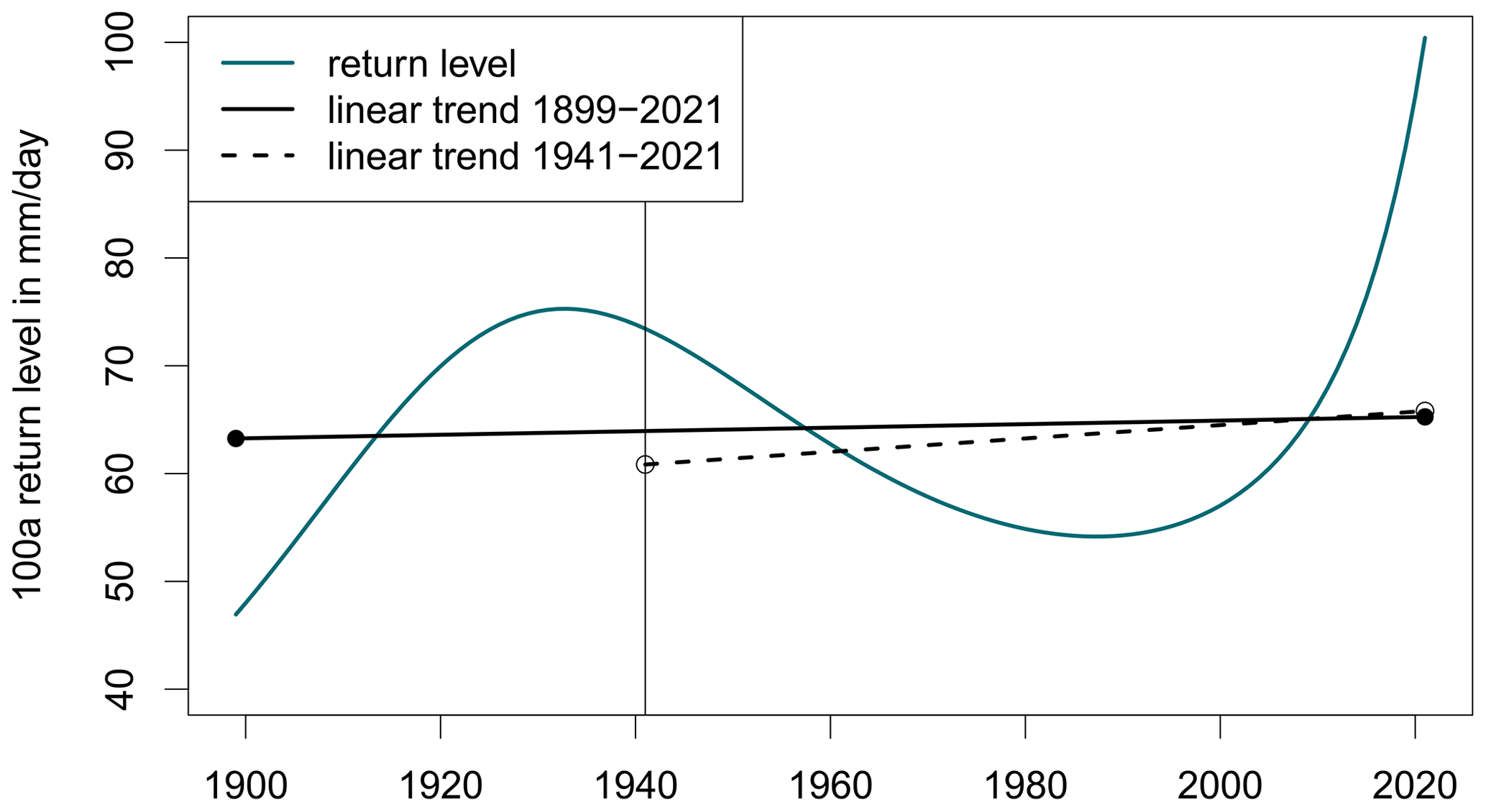
Figure A1The 100-year return level in millimeters per day (mm d−1) for station Krümmel (blue), the linear trend for the whole time period (black, solid) and the linear trend for the period 1941–2021 (black, dashed). Dots mark the first and the last value of the respective regression line.
Figures B1 and B2 show the relative changes in the 2-year return level (p=0.5) and the 100-year return level (p=0.99) for the 338 stations with interannual variations. Changes are regionally divergent; however, several contiguous regions are visible.
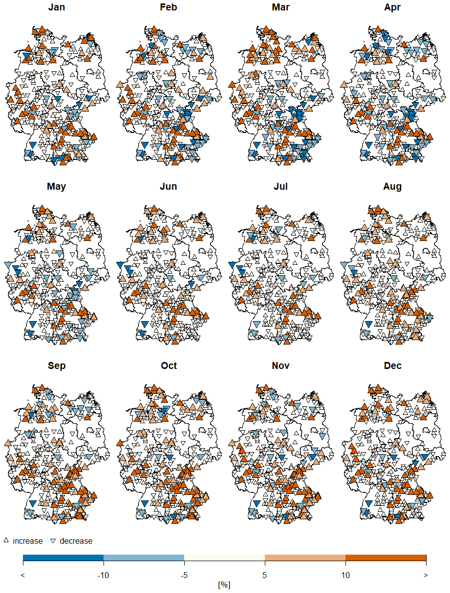
Figure B1Relative change from 1941 to 2021 for the 2-year return level (non-exceedance probability of p=0.5) for 338 stations. Increases/decreases are marked with triangles pointing up/triangles pointing down. Minor changes (< 5 %) remain uncolored with small symbols; stronger increases/decreases are highlighted in orange/blue.
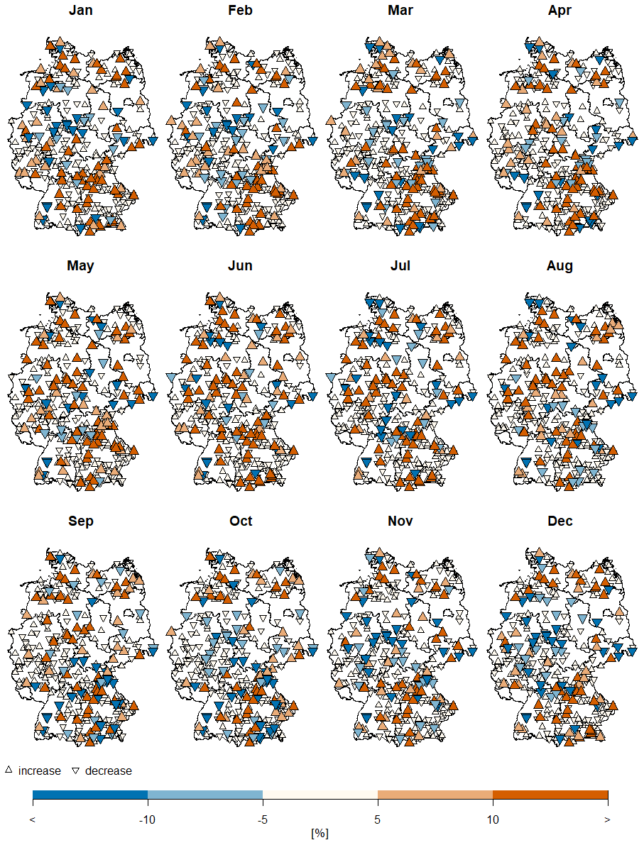
Figure B2Relative change from 1941 to 2021 for the 100-year return level (non-exceedance probability of p=0.99) for 338 stations. Increases/decreases are marked with triangles pointing up/triangles pointing down. Minor changes (< 5 %) remain uncolored with small symbols; stronger increases/decreases are highlighted in orange/blue.
According to Rootzén and Katz (2013), the design-life level is a measure to quantify risks for engineering design purposes in a changing climate. This measure can be regarded as a logical extension of the return level approach, which can only be meaningfully interpreted in a stationary setting. For example, a 100-year return level of extreme precipitation is the value which is expected to be exceeded on average once in hundred years. Due to changing climate, an event can occur in 2023 once every 100 years; in 2050 the same event might be exceeded on average once in 90 years. The changing return period (or exceedance probability) is an obstacle for engineering applications. One solution is given by the design-life level, which accounts for the time when the hydraulic system will be built and the service life of the system, called the design-life period. While the design-life period should be very long for dike design (e.g., 10 000 years in Netherlands (Botzen et al., 2009)), the service life of a rain gutter is much shorter.
The design-life level rp can be obtained by numerically optimizing the equation:
with Gi being the generalized extreme value distribution for year i, p the non-exceedance probability and I the design-life period. This approach assumes independent maxima. The design-life level is stated as T1−T2 (1−p) % extreme level, with indicating the start/end of the design-life period. To calculate future design-life levels, we use the seasonal–interannual and the seasonal-only model to extrapolate the parameters of the GEV for the month of July at the station Rain am Lech until 2051 (Fig. C1). With Eq. (C1), the 2022–2051 1 % extreme precipitation level (I=30 ,p=0.99) for the month of July at Rain am Lech obtained with the seasonal–interannual model equals to 161.4 mm d−1. In other words, there is a 1 in 100 risk that the largest daily precipitation event during 2022–2051 will be higher than 161.4 mm d−1. The 2022–2051 1 % extreme precipitation level for the seasonal-only approach is 132.5 mm d−1. If the detected trend at Rain am Lech continues for the years 2022–2051, as assumed here, the seasonal-only approach will lead to underestimated risks and the designed risk adaptation system will be strained beyond its planning purpose.
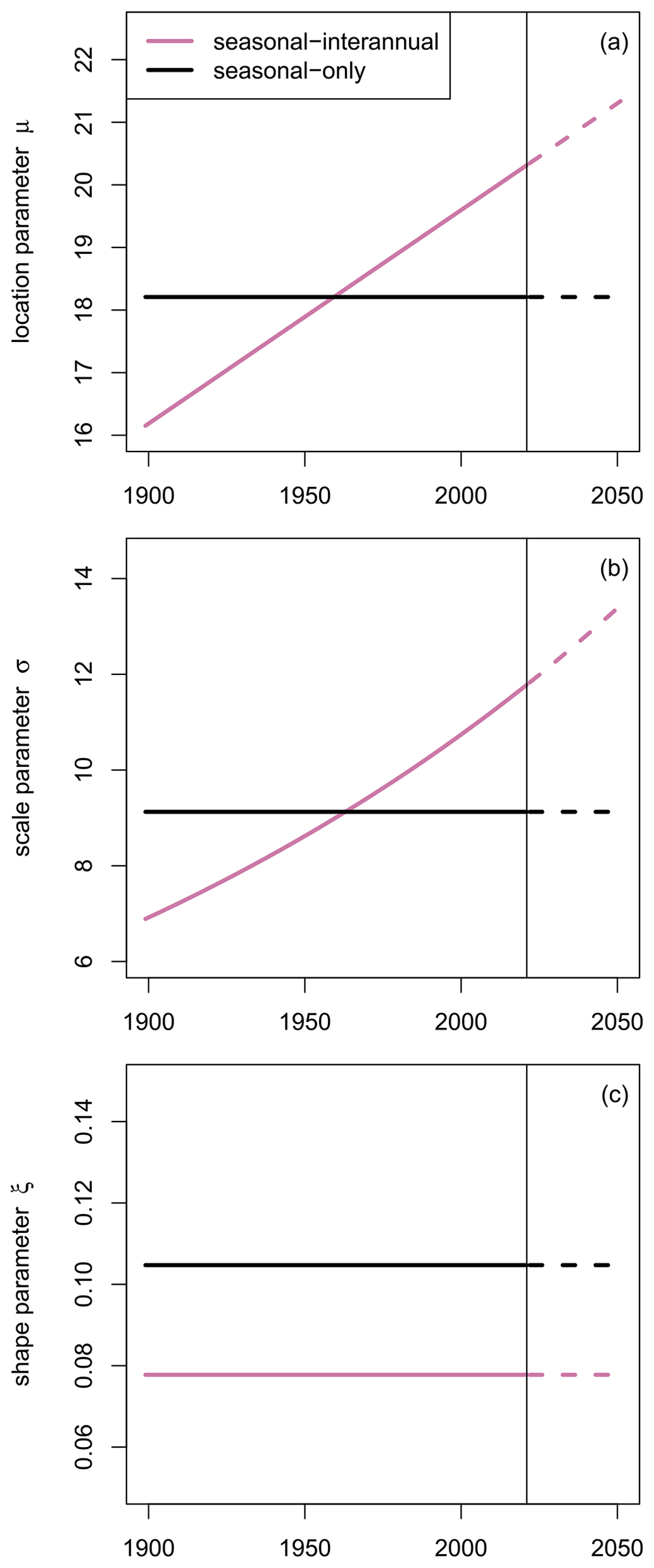
Figure C1Estimated parameter for location μ (a), scale σ (b) and shape ξ (c) at the example station Rain am Lech for the month of July using a seasonal–interannual model (pink) and a seasonal-only model (black). In addition to the estimates for the observation period (solid line), extrapolated values since 2022 are also illustrated (dashed lines).
The analysis was carried out using R, an environment for statistical computing and graphics (R Core Team, 2022), based on the VGAM package (Yee, 2015). The code remains unavailable to the public due to its extensive proprietary components and the utilization of numerous external libraries with varying dependencies. Furthermore, the code lacks the requisite documentation and comprehensive testing required for seamless integration into different environments or for other datasets. Regrettably, the constraints of resources within the scope of this scientific research have hindered the thorough preparation of the code for publication. In order to prevent potential misuse of the code in its current state, a decision has been made to withhold its publication. However, interested readers are welcome to reach out directly to the main author to inquire about accessing the underlying code and accompanying explanations.
Daily precipitation sums in Germany are provided by the National Climate Data Center of the German Weather Service (DWD) and are publicly accessible under https://opendata.dwd.de/climate_environment/CDC/observations_germany/climate/daily/more_precip/historical/ (DWD, 2023).
MP, HWR and UU designed the study concepts and methodology. MP conducted the analysis, generated the results and wrote the first draft. All authors contributed to writing the manuscript and approved the final version.
At least one of the (co-)authors is a member of the editorial board of Natural Hazards and Earth System Sciences. The peer-review process was guided by an independent editor, and the authors also have no other competing interests to declare.
Publisher’s note: Copernicus Publications remains neutral with regard to jurisdictional claims made in the text, published maps, institutional affiliations, or any other geographical representation in this paper. While Copernicus Publications makes every effort to include appropriate place names, the final responsibility lies with the authors.
We thank Oscar Jurado de Larios and Felix Fauer for proofreading and Theano Iliopoulou and the anonymous referee for their careful reading of our manuscript and their constructive comments.
This research has been supported by the Deutsche Forschungsgemeinschaft (grant no. GRK 2043/1) within the research training group NatRiskChange at Potsdam University.
The article processing charges for this open-access publication were covered by the Freie Universität Berlin.
This paper was edited by Piero Lionello and reviewed by Theano Iliopoulou and one anonymous referee.
Aleshina, M., Semenov, V., and Chernokulsky, A.: A link between surface air temperature and extreme precipitation over Russia from station and reanalysis data, Environ. Res. Lett., 16, 105004, https://doi.org/10.1088/1748-9326/ac1cba, 2021. a
Ambrosino, C., Chandler, R. E., and Todd, M. C.: Southern African monthly rainfall variability: An analysis based on generalized linear models, J. Climate, 24, 4600–4617, 2011. a
Arun, A., Haque, M. M., Lyon, C., Sayed, T., Washington, S., Loewenherz, F., Akers, D., Bandy, M., Bahl, V., Ananthanarayanan, G., and Shu, Y.: Leading Pedestrian Intervals – Yay or Nay? A Before-After Evaluation using Traffic Conflict-Based Peak Over Threshold Approach, https://bellevuewa.gov/sites/default/files/media/pdf_document/2022/leading-pedestrian-intervals-research-paper-010322.pdf (last access: 18 March 2024), 2022. a
Bahrami, M. and Mahmoudi, M. R.: Long-term temporal trend analysis of climatic parameters using polynomial regression analysis over the Fasa Plain, southern Iran, Meteorol. Atmos. Phys., 134, 1–12, 2022. a
Bentzien, S. and Friederichs, P.: Decomposition and graphical portrayal of the quantile score, Q. J. Roy. Meteor. Soc., 140, 1924–1934, 2014. a
Botzen, W. J. W., Aerts, J., and van den Bergh, J. C. J. M.: Dependence of flood risk perceptions on socioeconomic and objective risk factors, Water Resour. Res., 45, W10440, https://doi.org/10.1029/2009WR007743, 2009. a
Bousquet, N. and Bernardara, P.: Extreme Value Theory with Applications to Natural Hazards: From Statistical Theory to Industrial Practice, Springer Nature, https://doi.org/10.1007/978-3-030-74942-2, 2021. a
Byun, K. and Hamlet, A. F.: A risk-based analytical framework for quantifying non-stationary flood risks and establishing infrastructure design standards in a changing environment, J. Hydrol., 584, 124575, https://doi.org/10.1016/j.jhydrol.2020.124575, 2020. a
Casanueva, A., Rodríguez-Puebla, C., Frías, M. D., and González-Reviriego, N.: Variability of extreme precipitation over Europe and its relationships with teleconnection patterns, Hydrol. Earth Syst. Sci., 18, 709–725, https://doi.org/10.5194/hess-18-709-2014, 2014. a
Coles, S.: An Introduction to Statistical Modelling of Extreme Values, Springer, ISBN 1-85233-459-2, 2001. a, b, c
Davini, P. and d’Andrea, F.: From CMIP3 to CMIP6: Northern Hemisphere atmospheric blocking simulation in present and future climate, J. Climate, 33, 10021–10038, 2020. a
Derbile, E. K. and Kasei, R. A.: Vulnerability of crop production to heavy precipitation in north-eastern Ghana, Int. J. Clim. Chang. Str., 4, 36–53, 2012. a
Detring, C., Müller, A., Schielicke, L., Névir, P., and Rust, H. W.: Occurrence and transition probabilities of omega and high-over-low blocking in the Euro-Atlantic region, Weather Clim. Dynam., 2, 927–952, https://doi.org/10.5194/wcd-2-927-2021, 2021. a
DWD: KOSTRA-DWD-2000, Starkniederschlagshöhen für Deutschland–Grundlagenbericht, https://www.dwd.de/DE/fachnutzer/wasserwirtschaft/kooperationen/kostra/fortschreibung_pdf.pdf?__blob=publicationFile&v=3 (last access: 18 March 2024), 2000. a
DWD: Historical daily precipitation observations for Germany, Climate Data Center, v21.3 edn., https://opendata.dwd.de/climate_environment/CDC/observations_germany/climate/daily/more_precip/historical/DESCRIPTION_obsgermany_climate_daily_more_precip_historical_en.pdf (last access: 18 March 2024), 2021. a, b
DWD: Open-Data-Server, https://opendata.dwd.de/ (last access: 19 August 2022), 2022. a
DWD: Historical daily precipitation observations for Germany, Climate Data Center [data set], https://opendata.dwd.de/climate_environment/CDC/observations_germany/climate/daily/more_precip/historical/ (last access: 1 April 2024), 2023. a
DWD: KOSTRA DWD, https://www.dwd.de/DE/leistungen/kostra_dwd_rasterwerte/kostra_dwd_rasterwerte.html (last access: 26 January 2024), 2024. a
Embrechts, P., Klüppelberger, C., and Mikosch, T.: Modelling Extremal Events for Insurance and Fincance, Springer, Berlin, ISBN 3-540-60931-8, 1997. a
Fabozzi, F. J., Focardi, S. M., Rachev, S. T., and Arshanapalli, B. G.: The basics of financial econometrics: Tools, concepts, and asset management applications, John Wiley & Sons, ISBN 978-1-118-72743-0, 2014. a
Fauer, F. S. and Rust, H. W.: Non-stationary large-scale statistics of precipitation extremes in central Europe, Stoch. Environ. Res. Risk A., 37, 4417–4429, 2023. a
Fauer, F. S., Ulrich, J., Jurado, O. E., and Rust, H. W.: Flexible and consistent quantile estimation for intensity–duration–frequency curves, Hydrol. Earth Syst. Sci., 25, 6479–6494, https://doi.org/10.5194/hess-25-6479-2021, 2021. a
Ferreira, A., Friederichs, P., de Haan, L., Neves, C., and Schlather, M.: Estimating space-time trend and dependence of heavy rainfall, arXiv [preprint], https://doi.org/10.48550/arXiv.1707.04434, 2017. a
Fischer, M., Rust, H., and Ulbrich, U.: Seasonal Cycle in German Daily Precipitation Extremes, Meteorol. Z., 27, 3–13, https://doi.org/10.1127/metz/2017/0845, 2018. a, b, c, d, e, f, g
Fischer, M., Rust, H., and Ulbrich, U.: A spatial and seasonal climatology of extreme precipitation return-levels: a case study, Spatial Stat., 34, 100275, https://doi.org/10.1016/j.spasta.2017.11.007, 2019. a, b, c, d, e, f, g, h
Friederichs, P. and Hense, A.: Statistical downscaling of extreme precipitation events using censored quantile regression, Mon. Weather Rev., 135, 2365–2378, 2007. a
Galiatsatou, P. and Prinos, P.: Analysing the effects of climate change on wave height extremes in the Greek Seas, in: ICHE 2014, Proceedings of the 11th International Conference on Hydroscience & Engineering, Hamburg, Germany, Karlsruhe: Bundesanstalt für Wasserbau, 28 September–2 October 2014, https://henry.baw.de/server/api/core/bitstreams/f661f66a-6e72-4f28-9374-ea41bca97759/content (last access: 18 March 2024), 773–782, 2014. a
Gilli, M. and Këllezi, E.: An application of extreme value theory for measuring financial risk, Computat. Econ., 27, 207–228, 2006. a
Gkillas, K. and Katsiampa, P.: An application of extreme value theory to cryptocurrencies, Econ. Lett., 164, 109–111, 2018. a
Golroudbary, V. R., Zeng, Y., Mannaerts, C. M., and Su, Z. B.: Attributing seasonal variation of daily extreme precipitation events across The Netherlands, Weather and Climate Extremes, 14, 56–66, 2016. a, b
Hurrell, J. W.: Decadal trends in the North Atlantic Oscillation: Regional temperatures and precipitation, Science, 269, 676–679, 1995. a, b
Hurrell, J. W. and Deser, C.: North Atlantic climate variability: the role of the North Atlantic Oscillation, J. Marine Syst., 79, 231–244, 2010. a, b
Jurado, O. E., Oesting, M., and Rust, H. W.: Implications of modeling seasonal differences in the extremal dependence of rainfall maxima, Stoch. Environ. Res. Risk A., 37, 1963–1981, https://doi.org/10.1007/s00477-022-02375-z, 2022. a
Katz, R. W., Parlange, M. B., and Naveau, P.: Statistics of extremes in hydrology, Adv. Water Resour., 25, 1287–1304, 2002. a
Kjesbu, O., Witthames, P., Solemdal, P., and Walker, M. G.: Temporal variations in the fecundity of Arcto-Norwegian cod (Gadus morhua) in response to natural changes in food and temperature, J. Sea Res., 40, 303–321, 1998. a
Łupikasza, E. B.: Seasonal patterns and consistency of extreme precipitation trends in Europe, December 1950 to February 2008, Clim. Res., 72, 217–237, 2017. a, b, c, d
Maraun, D., Rust, H. W., and Osborn, T. J.: The annual cycle of heavy precipitation across the UK: a model based on extreme value statistics, J. Climatol., 29, 1731–1744, 2009. a, b, c
Maraun, D., Rust, H. W., and Osborn, T. J.: The influence of synoptic airflow on UK daily precipitation extremes. Part I: observed spatio-temporal relations, Clim. Dynam., 36, 261–275, 2011. a
Méndez, F. J., Menéndez, M., Luceño, A., and Losada, I. J.: Analyzing monthly extreme sea levels with a time-dependent GEV model, J. Atmos. Ocean. Tech., 24, 894–911, 2007. a
Min, J. L. J. and Halim, S. A.: Rainfall Modelling using Generalized Extreme Value Distribution with Cyclic Covariate, Mathematics and Statistics, 8, 762–772, https://doi.org/10.13189/ms.2020.080617, 2020. a
Moghaddasi, M., Anvari, S., and Mohammadi, T.: Comparison of extreme value theory approaches in temperature frequency analysis (case study: Arak plain in Iran), Arab. J. Geosci., 15, 1–13, 2022. a
Mondal, A. and Daniel, D.: Return levels under nonstationarity: The need to update infrastructure design strategies, J. Hydrol. Eng., 24, 04018060, https://doi.org/10.1061/(ASCE)HE.1943-5584.0001738, 2019. a
Mudelsee, M.: Trend analysis of climate time series: A review of methods, Earth-Sci. Rev., 190, 310–322, 2019. a
Naveau, P., Nogaj, M., Ammann, C., Yiou, P., Cooley, D., and Jomelli, V.: Statistical methods for the analysis of climate extremes, C. R. Geosci., 337, 1013–1022, 2005. a
Neath, A. A. and Cavanaugh, J. E.: The Bayesian information criterion: background, derivation, and applications, Wires Comput. Mol. Sci., 4, 199–203, 2012. a
Papalexiou, S. M. and Koutsoyiannis, D.: Battle of extreme value distributions: A global survey on extreme daily rainfall, Water Resour. Res., 49, 187–201, 2013. a, b, c
Pinto, J. G., Ulbrich, U., Leckebusch, G. C., Spangehl, T., Reyers, M., and Zacharias, S.: Changes in storm track and cyclone activity in three SRES ensemble experiments with the ECHAM5/MPI-OM1 GCM, Clim. Dynam., 29, 195–210, 2007. a
Pinto, J. G., Zacharias, S., Fink, A. H., Leckebusch, G. C., and Ulbrich, U.: Factors contributing to the development of extreme North Atlantic cyclones and their relationship with the NAO, Clim. Dynam., 32, 711–737, 2009. a
Pörtner, H.-O., Roberts, D. C., Tignor, M., Poloczanska, E. S., Mintenbeck, K., Alegría, A., Craig, M., Langsdorf, S., Löschke, S., Möller, V., Okem, A., and Rama, B. (Eds.): Climate change 2022: Impacts, adaptation and vulnerability, Cambridge University Press, Cambridge, UK and New York, NY, USA, https://doi.org/10.1017/9781009325844, 2022. a, b
Priestley, M. B.: Spectral Analysis and Time Series, Academic Press, London, ISBN 0-12-564922-3, 1992. a
R Core Team: R: A Language and Environment for Statistical Computing, R Foundation for Statistical Computing, Vienna, Austria, https://www.R-project.org/ (last access: 18 March 2024), 2022. a
Ragulina, G. and Reitan, T.: Generalized extreme value shape parameter and its nature for extreme precipitation using long time series and the Bayesian approach, Hydrolog. Sci. J., 62, 863–879, 2017. a
Rajczak, J., Pall, P., and Schär, C.: Projections of extreme precipitation events in regional climate simulations for Europe and the Alpine Region, J. Geophys. Res.-Atmos., 118, 3610–3626, 2013. a
Ribereau, P., Naveau, P., and Guillou, A.: A note of caution when interpreting parameters of the distribution of excesses, Adv. Water Resour., 34, 1215–1221, https://doi.org/10.1016/j.advwatres.2011.05.003, 2011. a
Richling, A., Grieger, J., and Rust, H. W.: Decomposition of skill scores for conditional verification – Impact of AMO phases on the predictability of decadal temperature forecasts, EGUsphere [preprint], https://doi.org/10.5194/egusphere-2023-2582, 2024. a
Rootzén, H. and Katz, R. W.: Design life level: quantifying risk in a changing climate, Water Resour. Res., 49, 5964–5972, 2013. a, b, c
Rosenzweig, C., Tubiello, F. N., Goldberg, R., Mills, E., and Bloomfield, J.: Increased crop damage in the US from excess precipitation under climate change, Global Environ. Chang., 12, 197–202, 2002. a
Rust, H. W.: The Effect of Long-Range Dependence on Modelling Extremes with the Generalised Extreme Value Distribution, Eur. Phys. J.-Spec. Top., 174, 91–97, 2009. a
Rust, H. W., Maraun, D., and Osborn, T. J.: Modelling Seasonality in Extreme Rainfall: a UK case study, Eur. Phys. J.-Spec. Top., 174, 99–111, 2009. a, b, c
Rust, H. W., Vrac, M., Sultan, B., and Lengaigne, M.: Mapping weather-type influence on Senegal precipitation based on a spatial-temporal statistical model, J. Climate, 26, 8189–8209, 2013. a, b
Shacham, M. and Brauner, N.: Minimizing the effects of collinearity in polynomial regression, Ind. Eng. Chem. Res., 36, 4405–4412, 1997. a
Szigeti, M., Ferenci, T., and Kovács, L.: The use of peak over threshold methods to characterise blood glucose curves, in: 2020 IEEE 14th International Symposium on Applied Computational Intelligence and Informatics (SACI), IEEE, Timişoara, Romania, 21–23 May 2020, 000199–000204, https://real.mtak.hu/121217/1/szigeti2020SACI.pdf (last access: 20 March 2024), 2020. a
Teegavarapu, R. S. V.: Floods in a changing climate: extreme precipitation, Cambridge University Press, ISBN 978-1-107-01878-5, 2012. a
Thomson, R., Drynan, L., and Veldema, A.: Australian Rainfall and Runoff Revision Project 20: Risk Assessment and Design Life, https://arr.ga.gov.au/__data/assets/pdf_file/0003/40548/ARR_Project_20_Stage3_Report.pdf (last access: 20 March 2024), 2015. a
Trenberth, K. E., Dai, A., Rasmussen, R. M., and Parsons, D. B.: The changing character of precipitation, B. Am. Meteorol. Soc., 84, 1205–1218, 2003. a
Trenczek, J., Lühr, O., Eiserbeck, L., Sandhövel, M., and Leuschner, V.: Übersicht vergangener Extremwetterschäden in Deutschland, https://www.prognos.com/de/projekt/bezifferung-von-klimafolgekosten-deutschland (last access: 20 March 2024) 2022. a
Ulrich, J., Jurado, O. E., Peter, M., Scheibel, M., and Rust, H. W.: Estimating IDF curves consistently over durations with spatial covariates, Water, 12, 3119, https://doi.org/10.3390/w12113119, 2020. a, b, c
Ulrich, J., Fauer, F. S., and Rust, H. W.: Modeling seasonal variations of extreme rainfall on different timescales in Germany, Hydrol. Earth Syst. Sci., 25, 6133–6149, https://doi.org/10.5194/hess-25-6133-2021, 2021. a, b, c
Villafuerte, M. Q., Matsumoto, J., and Kubota, H.: Changes in extreme rainfall in the Philippines (1911–2010) linked to global mean temperature and ENSO, Int. J. Climatol., 35, 2033–2044, 2015. a
Vormoor, K., Lawrence, D., Heistermann, M., and Bronstert, A.: Climate change impacts on the seasonality and generation processes of floods – projections and uncertainties for catchments with mixed snowmelt/rainfall regimes, Hydrol. Earth Syst. Sci., 19, 913–931, https://doi.org/10.5194/hess-19-913-2015, 2015. a
Seneviratne, S. I., Zhang, X., Adnan, M., Badi, W., Dereczynski, C., Di Luca, A., Ghosh, S., Iskandar, I., Kossin, J., Lewis, S., Otto, F., Pinto, I., Satoh, M., Vicente-Serrano, S. M., Wehner, M., and Zho, B.: Weather and climate extreme events in a changing climate, in: Climate Change 2021: The Physical Science Basis. Contribution of Working Group I to the Sixth Assessment Report of the Intergovernmental Panel on Climate Change, Cambridge University Press, Cambridge, United Kingdom and New York, NY, USA, 1513–1766, https://doi.org/10.1017/9781009157896.013, 2021. a
Westra, S., Alexander, L. V., and Zwiers, F. W.: Global increasing trends in annual maximum daily precipitation, J. Climate, 26, 3904–3918, 2013. a
Westra, S., Fowler, H. J., Evans, J. P., Alexander, L. V., Berg, P., Johnson, F., Kendon, E. J., Lenderink, G., and Roberts, N.: Future changes to the intensity and frequency of short-duration extreme rainfall, Rev. Geophys., 52, 522–555, 2014. a, b
Willems, P.: Multidecadal oscillatory behaviour of rainfall extremes in Europe, Climatic Change, 120, 931–944, 2013. a, b, c, d
WMO: Guide to meteorological instruments and methods of observation, ISBN 978-92-63-100085, https://www.weather.gov/media/epz/mesonet/CWOP-WMO8.pdf (last access: 20 March 2024), 1996. a
Xu, P., Wang, D., Singh, V. P., Wang, Y., Wu, J., Lu, H., Wang, L., Liu, J., and Zhang, J.: Time-varying copula and design life level-based nonstationary risk analysis of extreme rainfall events, Hydrol. Earth Syst. Sci. Discuss. [preprint], https://doi.org/10.5194/hess-2019-358, 2019. a
Yee, T. W.: Vector Generalized Linear and Additive Models: With an Implementation in R, Springer, New York, USA, ISBN 978-1-4939-2817-0, 2015. a, b, c
Yiou, P., Ribereau, P., Naveau, P., Nogaj, M., and Brázdil, R.: Statistical analysis of floods in Bohemia (Czech Republic) since 1825, Hydrolog. Sci. J., 51, 930–945, 2006. a
Zeder, J. and Fischer, E. M.: Observed extreme precipitation trends and scaling in Central Europe, Weather and Climate Extremes, 29, 100266, https://doi.org/10.1016/j.wace.2020.100266, 2020. a, b, c
Zeppel, M. J. B., Wilks, J. V., and Lewis, J. D.: Impacts of extreme precipitation and seasonal changes in precipitation on plants, Biogeosciences, 11, 3083–3093, https://doi.org/10.5194/bg-11-3083-2014, 2014. a
Zolina, O., Simmer, C., Kapala, A., Bachner, S., Gulev, S., and Maechel, H.: Seasonally dependent changes of precipitation extremes over Germany since 1950 from a very dense observational network, J. Geophys. Res.-Atmos., 113, D06110, https://doi.org/10.1029/2007JD008393, 2008. a, b, c, d
- Abstract
- Introduction
- Data
- Modeling seasonal–interannual extreme precipitation
- Model building and verification
- Gain of interannual variability
- Importance of a flexible shape parameter
- Impact of climate change on the seasonality of extreme precipitation
- Conclusion
- Appendix A: Linear trends in return levels and phase
- Appendix B: Maps of relative changes in return levels
- Appendix C: Design-life level
- Code availability
- Data availability
- Author contributions
- Competing interests
- Disclaimer
- Acknowledgements
- Financial support
- Review statement
- References