Anticipating a risky future: long short-term memory (LSTM) models for spatiotemporal extrapolation of population data in areas prone to earthquakes and tsunamis in Lima, Peru

In this paper, we anticipate geospatial population distributions to quantify the future number of people living in earthquake-prone and tsunami-prone areas of Lima and Callao, Peru. We capitalize upon existing gridded population time series data sets, which are provided on an open-source basis globally, and implement machine learning models tailored for time series analysis, i.e., based on long short-term memory (LSTM) networks, for prediction of future time steps. Specifically, we harvest WorldPop population data and teach LSTM and convolutional LSTM models equipped with both unidirectional and bidirectional learning mechanisms, which are derived from different feature sets, i.e., driving factors. To gain insights regarding the competitive performance of LSTM-based models in this application context, we also implement multilinear regression and random forest models for comparison. The results clearly underline the value of the LSTM-based models for forecasting gridded population data; the most accurate prediction obtained with an LSTM equipped with a bidirectional learning scheme features a root-mean-squared error of 3.63 people per 100 × 100 m grid cell while maintaining an excellent model fit (R²= 0.995). We deploy this model for anticipation of population along a 3-year interval until the year 2035. Especially in areas of high peak ground acceleration of 207–210 cm s⁻², the population is anticipated to experience growth of almost 30 % over the forecasted time span, which simultaneously corresponds to 70 % of the predicted additional inhabitants of Lima. The population in the tsunami inundation area is anticipated to grow by 61 % until 2035, which is substantially more than the average growth of 35 % for the city. Uncovering those relations can help urban planners and policymakers to develop effective risk mitigation strategies.

1 Introduction

Socio-natural disasters represent a perpetual peril to humans. Such events frequently result in substantial losses. The anticipated growth of the world population with a peak of 9.7 billion people in the year 2050 (United Nations, 2022) is expected to expose more people to natural hazards than ever before (Iglesias et al., 2021; Cremen et al., 2022). The dynamic change in geospatial population distributions due to both population growth and urbanization processes (UN Habitat, 2016) demands a frequent update and anticipation of (future) geospatial population distributions in hazard-prone areas. Such an approach enables urban planners and policymakers to develop effective strategies for risk mitigation. This need is also embedded in the UN Sendai Framework for Disaster Risk Reduction, which explicitly stresses the importance of preparing for future socio-natural disasters via strategies that minimize uncontrolled settlement development in areas in peril (UNISDR, 2015).

As a key variable to characterize natural-hazard-related exposure, obtaining geospatial data on population distribution is essential. To anticipate future geospatial population distributions, different families of methods can generally be considered; rule-based methods establish a set of explicitly defined rules for transition trajectories over time. This family of methods contains (i) cellular automata techniques (Clarke, 2014), which represent discrete spatiotemporal dynamic systems based on local rules; (ii) agent-based modeling, which simulates dynamic interactions among agents in a virtual environment (Abar et al., 2017); and (iii) Markov chain models, which represent a stochastic process that produces sequential states in which each prediction is dependent on the previous state (Gagniuc, 2017).

However, especially recently, a second family of methods, i.e., techniques of machine learning (ML), was deployed for predicting transition trajectories in the context of population modeling. The underlying idea is to infer a decision rule (e.g., a function) from properly encoded prior knowledge (i.e., labeled training samples) related to time series data to predict changes (Zhu, 2023). For instance, Chen et al. (2020) integrate historical population maps and multiple machine learning algorithms, namely XGBoost, random forest (RF), and a multilayer perceptron neural network, to predict future built-up land and population distributions. Kubota et al. (2022) implemented a graph convolutional network for short-term population prediction based on population count data collected through mobile phone signals. Zheng and Zhang (2020) implement a convolutional LSTM (ConvLSTM) network for weekly population distribution prediction based on geolocated social media data, i.e., Tencent positioning data.

Generally, Earth observation is customarily used to measure changes on the land surface in a spatially continuous way over long time frames (Koehler and Künzer, 2020). Multiple authors have employed such data sets in combination with advanced ML techniques to anticipate land-use and land-cover expansion (e.g., Zhu et al., 2021a, b; Wang et al., 2022). By integrating Earth observation data, different initiatives offer continuous gridded geospatial population data over a long time frame; WorldPop (Lloyd et al., 2017; Stevens et al., 2015) and LandScan (Dobson et al., 2000) provide yearly geospatial population estimates starting in the year 2000. The data sets are created with a top-down approach by disaggregating census information based on Earth observation imagery and ancillary spatial covariates. In this study, from a data-oriented perspective, we make use of existing time series population data sets, which are provided on an open-source basis globally, to anticipate future geospatial population distributions along a 3-year interval up to the year 2035.

From a methodological point of view, we implement advanced ML models tailored for time series analysis, i.e., networks based on long short-term memory (LSTM; Hochreiter and Schmidhuber, 1997). We follow different model configurations to exploit the sequential nature of the training data; we use unidirectional and bidirectional learning mechanisms. The former mechanism analyzes the input data in a sequence from the first time step to the last, whereas the latter mechanism additionally considers the reversed sequence from the last time step to the first. Moreover, to explicitly enable spatiotemporal modeling, i.e., to encode topological and spatial contextual relationships, we also implement ConvLSTM models (Shi et al., 2015). Consequently, in the experimental evaluation, we exhaustively disentangle the prediction accuracies as a function of the actual prediction model; the learning mechanism; and the deployed driving factors, i.e., different feature sets used for the prediction. Experimental results are obtained from Peru's capital Lima and Callao, which features a high population dynamic. To gain an insight into the competitive performance of LSTM-based models in this application context, we also deploy multilinear regression (MLR) and RF models for comparison.

Regarding the application context of this study, only a few works have explicitly focused on applying time series ML methods for mapping future natural-hazard-related exposure and vulnerability. For instance, Johnson et al. (2021) simulated future changes in urban land use up to the year 2050 with a trend-based logistic regression cellular automaton model and evaluated potential flood exposure for the Philippines. Scheuer et al. (2021) modeled residential-choice behavior on a city level and examined how this process could translate into future trends regarding exposure, vulnerability, and risk. Calderon and Silva (2021) forecasted the spatial distribution of the population and residential buildings for the assessment of future seismic risk based on geographically weighted regression and multi-agent systems for Costa Rica. Here, from an epistemological point of view, we uniquely combine the forecasted population data with earthquake and tsunami hazard models to quantify the future number of people living in earthquake-exposed and tsunami-exposed areas in Lima and Callao, Peru.

The remainder of the paper is organized as follows. In Sect. 2 we detail the proposed methodology. We describe the study area and experimental setup in Sect. 3. Experimental results are revealed in Sect. 4, and concluding remarks are given in Sect. 5.

2 Material and methods

Figure 1 provides an overview of the proposed workflow for the spatiotemporal forecasting of population data and quantification of exposure. First, multitemporal gridded population data are compiled and aligned to a set of geospatial covariates, i.e., driving factors. The data are fed into the LSTM-based models to establish a population forecast. The modeled future population is utilized with hazard models to quantify the number of people living in earthquake-exposed and tsunami-exposed areas in Lima and Callao, Peru, in the year 2035.

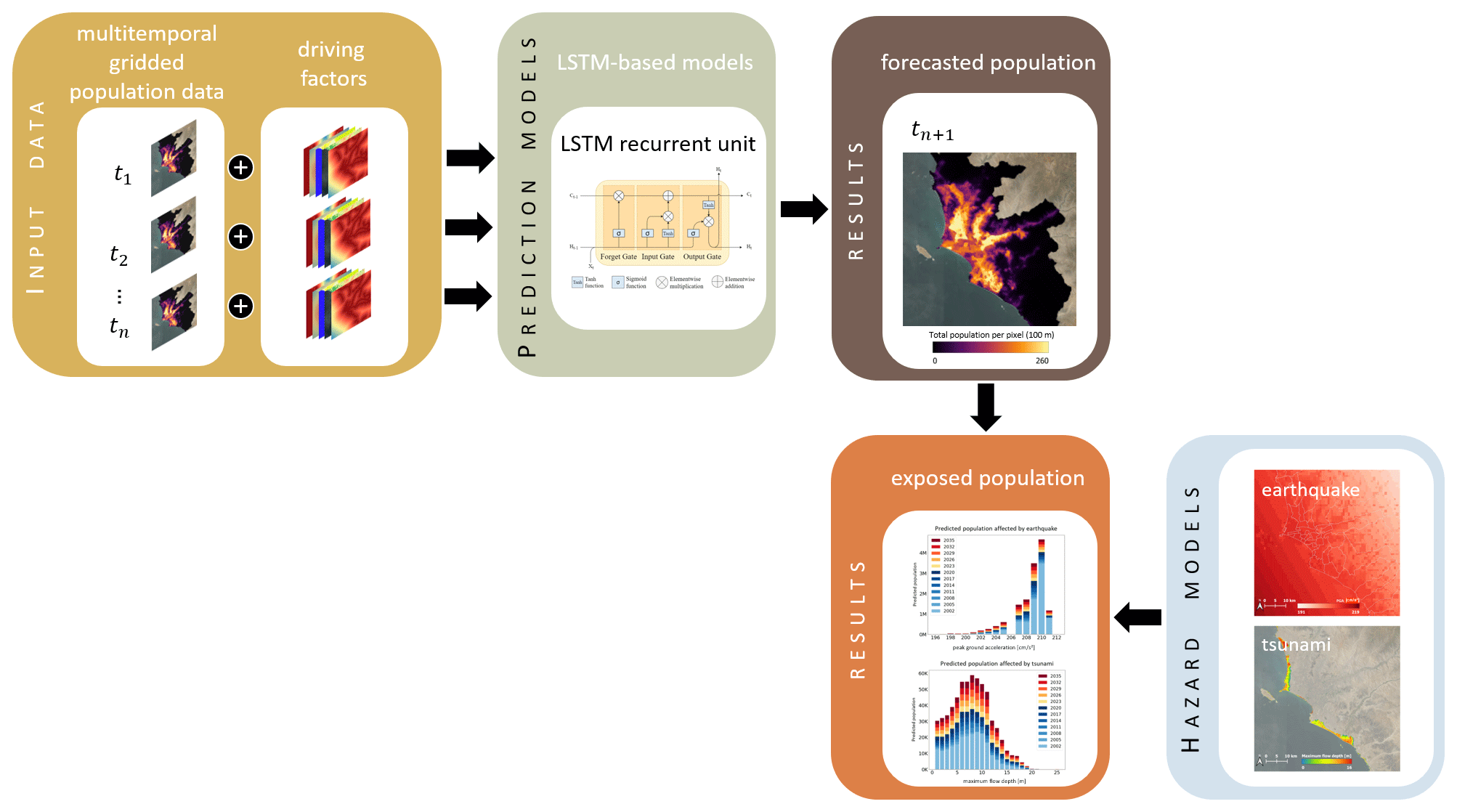
Figure 1 General workflow for the spatiotemporal forecasting of population data in earthquake- and tsunami-exposed areas of Lima and Callao, Peru.

2.1 Multitemporal gridded population data

As the key input variable for the spatiotemporal forecasting of population, we harvest multitemporal gridded population data from the WorldPop initiative (Lloyd et al., 2017; Stevens et al., 2015). The data set consists of annual multitemporal gridded population data with a spatial resolution of 100 m for the period 2000–2020, which describes the residential population (Fig. 2). Thereby, WorldPop provides population counts adjusted to the United Nations population estimations (United Nations, 2022). The data set was created with a regression-tree-based semi-automated dasymetric modeling approach. First, a weighting layer was created with an RF approach and multiple spatial covariates, including country-specific census counts; land cover; digital elevation models (DEMs); nighttime lights; net primary productivity; weather data; road networks; bodies of water and waterways; protected areas; and “facility” locations such as hospitals and schools. The modeled layer was subsequently deployed to perform a dasymetric redistribution of the census counts at a country level (Stevens et al., 2015). Actual census counts are redistributed from the smallest available administrative unit to the population grid with a higher spatial resolution. The modeled layer determines the weight of the population for each grid cell. Figure 2 also displays the absolute population change per grid cell for the time interval 2000–2020. It is traceable that the core of the settlement area faced a decrease in population, while the vast majority of grid cells document an increase in population over the last 2 decades.

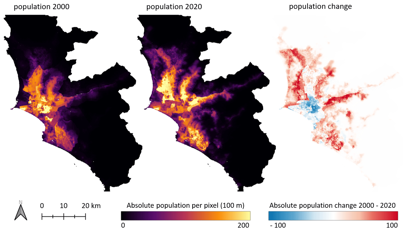
Figure 2 Starting point (population of the year 2000) and end point (population of the year 2020) of the annual gridded WorldPop population time series data, which serve as input for the forecasting models, and the corresponding visualized absolute population change between 2000–2020 for Lima and Callao, Peru.

2.2 Driving factors

We compute a set of geospatial covariates, i.e., driving factors, for spatiotemporal forecasting of population data. The driving factors are either time-variant or time-invariant (Fig. 3). Time-variant driving factors vary substantially over time and thus must be computed consistently along the timely resolution of the time series data, whereas the latter remain rather static over time. Land cover is an important driving factor for describing urban dynamics. The Moderate Resolution Imaging Spectroradiometer (MODIS) land cover data (Fig. 3a) from the National Aeronautics and Space Administration (NASA) have been provided annually since 2001 and thus match the temporal resolution of the population data (Friedl and Sulla-Menashe, 2019). We group the thematic classes of the data set into four distinctive categories, namely “vegetation”, “built-up”, “barren”, and “water”. From this multi-class data set, we create one-hot layers for each of the four thematic classes to be used as input for the models. Besides, the data feature a spatial resolution of 500 m, which corresponds to the coarsest resolution of all input features used. Consequently, we compute the second time-variant driving factor, i.e., distance to the boundary of built-up areas (Fig. 3b) based on the Euclidean distance function, by deploying the higher spatially resolved multitemporal gridded population data sets (Sect. 2.1). One very important geographic input factor for modeling population dynamics is the topography of the terrain, since human settlements mostly appear on terrains with flat or solely moderate slopes (Dobson et al., 2000). In this study, we use the Copernicus DEM (ESA, 2022), provided by the European Space Agency (ESA), with a spatial resolution of 30 m to compute slope estimates (Fig. 3c). The Copernicus DEM data set also contains information about bodies of water. We combine the data with the information on the bodies of water contained in the OpenStreetMap (OSM) data set (2022) to compute a layer indicating the distance to bodies of water for the study area (Fig. 3d). The OSM data set also served for the compilation of geospatial vector data representing roads and computing distances thereof (Fig. 3e). Lastly, we also compute a distance grid to the city center. In this study, we define the center of our study area as the point coordinate situated between the current central business district and the historic city center, i.e., the centro histórico of Lima (Fig. 3f). The compilation of a set of geospatial covariates that enables accurate estimations is a frequent challenge. For instance, Zhu (2023) lists more than 50 predictor variables which were employed in existing studies of land-use and land-cover predictions. Here, the collected driving factors represent frequently adopted variables in past studies (Gómez et al., 2020; Liu et al., 2017; Pijanowski et al., 2002). In detail, we internalize the main variable categories (Zhu, 2023), i.e., land-use-related variables (Fig. 3a–b, f), environmental variables (Fig. 3c, d), and infrastructural variables (Fig. 3e), as well as socio-economic variables (Fig. 2).

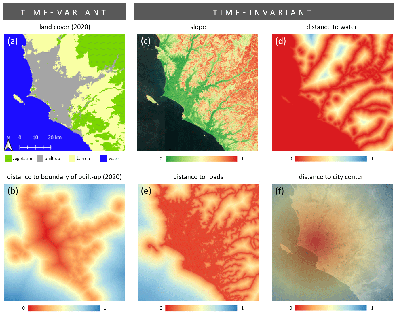
Figure 3 Driving factors deployed for the spatiotemporal forecasting of population data.

2.3 LSTM-based models

The population data of time steps $t_{\mathrm{1}},t_{\mathrm{2}},\mathrm{\dots },t_n$ and the corresponding driving factors are concatenated as the input for the LSTM models, which map the input to a prediction of the population at time step t_n+1. Generally, LSTM models belong to the family of recurrent neural networks (RNNs). The latter represents a generalization of feedforward neural networks with internal memory and which are designed to process sequential information (Rumelhart et al., 1986). RNNs model the input as sequentially arranged time steps while preserving the information of each past element as state memory in the hidden unit (LeCun et al., 2015). Such networks are referred to as recurrent, since the architecture is repeated over the time steps, whereby the weights are shared among the different temporal layers and the underlying function remains fixed over all time steps (Aggarwal, 2018). However, Hochreiter and Schmidhuber (1997) introduced LSTM networks to overcome the problem of vanishing gradients. LSTM networks are equipped with complex blocks as hidden layers. Those blocks implement gates and memory cells, which control the flow of information and accumulate the state information in order to obtain the capability of long-term memory. The blocks or the so-called “LSTM-cells” contain an internal recurrence mechanism additional to the outer recurrence mechanism of the RNN (Goodfellow et al., 2016). Thus, LSTMs can be considered for sequence learning and forecasting, especially when long-term dependencies should be encoded from the input data. The main model architecture comprises an LSTM unit with the following equations:

$$\begin{array}{}\text{(1)}& \begin{array}{rl}& i_t=\mathit{\sigma }({\mathbf{W}}_{xi}{X}_t+{\mathbf{W}}_{hi}{H}_{t-\mathrm{1}}+{\mathbf{W}}_{ci}\circ C_{t-\mathrm{1}}+b_i),\\ & f_t=\mathit{\sigma }({\mathbf{W}}_{xf}{X}_t+{\mathbf{W}}_{hf}{H}_{t-\mathrm{1}}+{\mathbf{W}}_{cf}\circ C_{t-\mathrm{1}}+b_f),\\ & C_t=f_t\circ C_{t-\mathrm{1}}+i_t\circ \tanh ({\mathbf{W}}_{xc}{X}_t+{\mathbf{W}}_{hc}{X}_{t-\mathrm{1}}+b_c),\\ & o_t=\mathit{\sigma }({\mathbf{W}}_{xo}{X}_t+{\mathbf{W}}_{ho}{H}_{t-\mathrm{1}}+{\mathbf{W}}_{co}\circ C_t+b_o),\\ & H_t=o_t\circ \tanh \left(C_t\right),\end{array}\end{array}$$

where X_t represents the input to the cell, C_t the memory state, and H_t the hidden state. The notation ∘ denotes the Hadamard product or the element-wise product. In the equations, i_t, f_t, and o_t refer to the input, forget, and output gates, respectively. Subscript t is the time step, σ the sigmoid activation function, tanh the hyperbolic tangent function, W the weight matrices, and b the biases (Fig. 4a).

To enable spatiotemporal modeling, we also employed ConvLSTMs. ConvLSTMs further contain convolutional structures with respect to both the input-to-state and state-to-state transitions. Thus, ConvLSTMs predict the future state of an entity (e.g., image pixel) from the current and past states of its surrounding entities (Shi et al., 2015). The inputs, cell outputs, hidden states, and gates are three-dimensional tensors with rows and columns of the two-dimensional input image as the last two dimensions. The internal operations use convolutions, which encode the spatial information (Shi et al., 2015). The architecture of a ConvLSTM is similar to an LSTM with the addition of the convolutional operator (Fig. 4b). Equations in Eq. (2) describe the ConvLSTM, which differ from the LSTM equations in the convolution operator denoted by ^*:

$$\begin{array}{}\text{(2)}& \begin{array}{rl}& i_t=\mathit{\sigma }\left({\mathbf{W}}_{xi}{}^{*}{X}_t+{\mathbf{W}}_{hi}{}^{*}{H}_{t-\mathrm{1}}+{\mathbf{W}}_{ci}\circ C_{t-\mathrm{1}}+b_i\right),\\ & f_t=\mathit{\sigma }({\mathbf{W}}_{xf}^{*}{X}_t+{\mathbf{W}}_{hf}{}^{*}{H}_{t-\mathrm{1}}+{\mathbf{W}}_{cf}\circ C_{t-\mathrm{1}}+b_f),\\ & C_t=f_t\circ C_{t-\mathrm{1}}+i_t\circ \tanh ({\mathbf{W}}_{xc}{}^{*}{X}_t+{\mathbf{W}}_{hc}{}^{*}{X}_{t-\mathrm{1}}+b_c),\\ & o_t=\mathit{\sigma }({\mathbf{W}}_{xo}{}^{*}{X}_t+{\mathbf{W}}_{ho}^{*}{H}_{t-\mathrm{1}}+{\mathbf{W}}_{co}\circ C_t+b_o),\\ & H_t=o_t\circ \tanh \left(C_t\right).\end{array}\end{array}$$

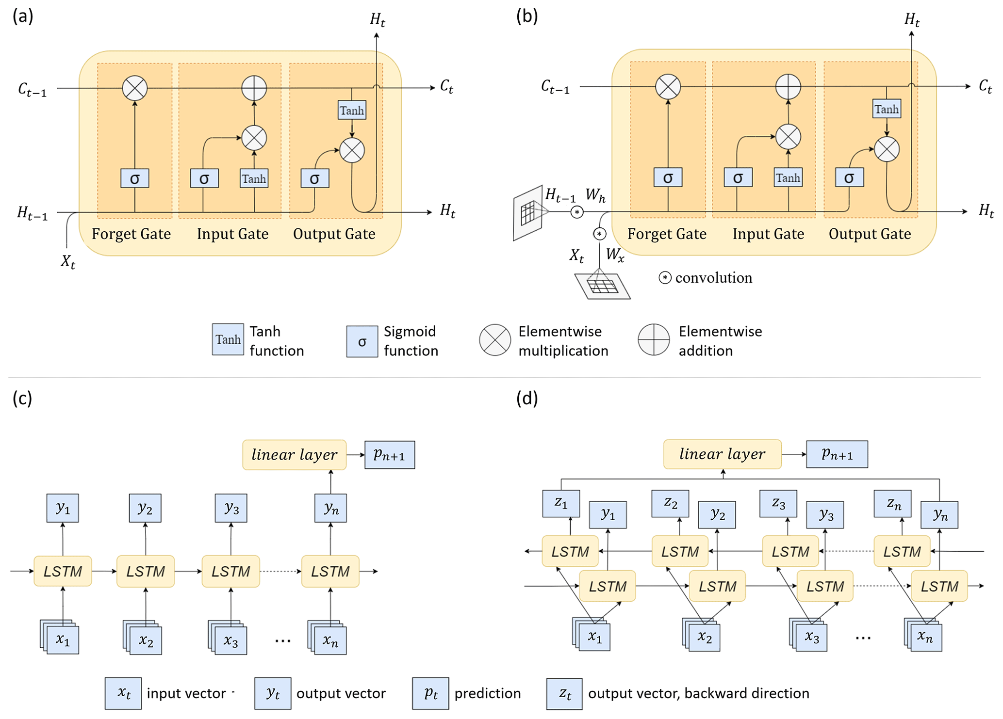
Figure 4 Implemented LSTM components and network architectures: (a) LSTM cell, (b) ConvLSTM cell, (c) unidirectional forward network, and (d) bidirectional network.

In this study, we train both models with a unidirectional forward (Fig. 4c) and bidirectional (Fig. 4d) learning mechanism. Vector x_t refers to the input data stacks for the chosen input years, i.e., $x_{\mathrm{1}},x_{\mathrm{2}},x_{\mathrm{3}},\mathrm{\dots },x_n$. Vectors y_t and z_t are the generated output vectors at each time step, with the chosen hidden dimension of 64. For the bidirectional network, the forward layer outputs y_t are computed iteratively using the input data in a sequence from the first time step to the last, while the backward layer outputs z_t are calculated from a reversed sequence of the inputs from the last time step to the first. To retrieve a one-dimensional output that represents the predicted population number p_n+1 at time step n+1, a linear layer is applied to the last output vectors. For the bidirectional networks, the last outputs y_n and z_n are concatenated. The ConvLSTM networks have the same architecture as in Fig. 4c–d but with convolutional operations included in the ConvLSTM cells as shown in Fig. 4b.

2.4 Hazard models: earthquake and tsunami

The RIESGOS 2.0 project, which focuses on the creation of scenario-based multi-risk assessment in the Andes region, provided earthquake and tsunami simulation data for this study (RIESGOS, 2022). The simulations are based on the historical earthquake of the year 1746 with an offshore epicenter and a magnitude of 8.9 (Gomez-Zapata et al., 2021). To assess the population affected by this earthquake and the corresponding tsunami, spatially distributed peak ground accelerations (Fig. 5a) and maximum flow depths (Fig. 5b) are used, respectively. The ground motion fields are generated based on ground motion prediction equations according to Montalva et al. (2017). The tsunami simulations (Androsov et al., 2023) are based on parameters proposed by Jimenez et al. (2013). The two data sets are provided with 1 km and 10 m spatial resolution, respectively, and we resample the data sets to the spatial resolution of 100 m of the population grid for the exposure analysis.

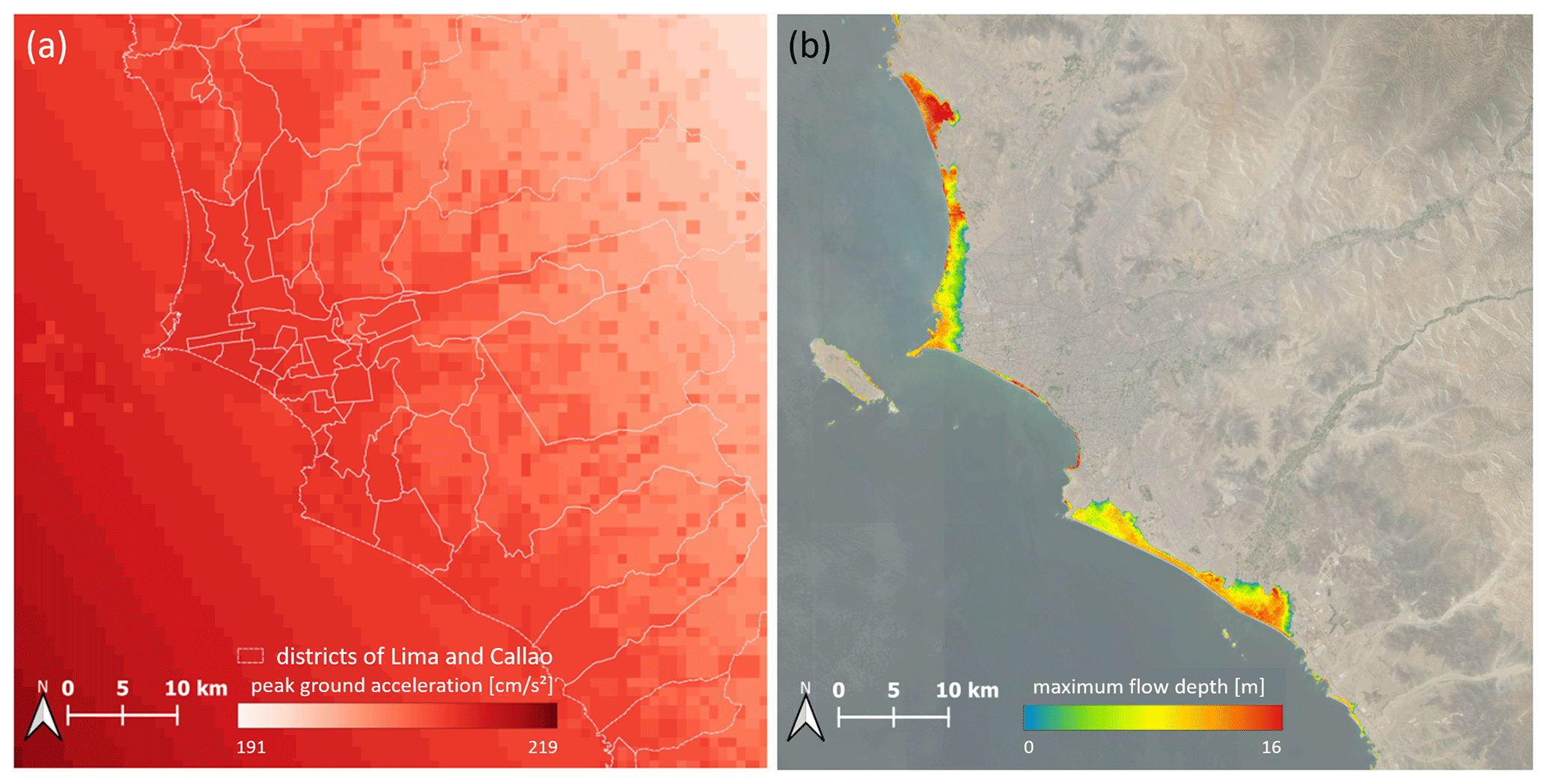
Figure 5 Considered hazard models: (a) the peak ground acceleration characterizing the historical earthquake of 1746 with an offshore epicenter and a magnitude of 8.9 and (b) the corresponding tsunami characterized by maximum flow depth.

3 Experimental setup

As previously mentioned, the study area comprises the settlement area of Peru's capital Lima and the neighboring province of Callao, which has a spatial coverage of approximately 6500 km². We re-project all data sets to the WorldPop projection EPSG:4326, i.e., the World Geodetic System 1984, and resample them to the spatial resolution of 100 m, which corresponds to the gridded population data. We normalize all layers individually and stack them to a multidimensional array of the shape (20, 10, 888, 888). Thereby, the first position carries the 20 years of gridded population data, whereas the second position contains the driving factors while establishing an image size of 888 × 888 elements. The WorldPop time series data are deployed along a 3-year interval (which provides an acceptable tradeoff here between the forecasting capability of the model and having a sufficient number of time steps available for training the model) and split into a training data set and validation data set along the temporal dimension. The training data set contains the earlier six time steps (2002, 2005, …, 2017), whereas the validation data set contains the later six time steps (2005, 2008, …, 2020) of the time series. In both training and validation data sets, we used the variables of the first five time steps as input and the last time step as the ground truth. As such, the target of the training data set is to predict the population of the year 2017, and the goal of the validation data set is to forecast the population map for the year 2020 (Fig. 6).

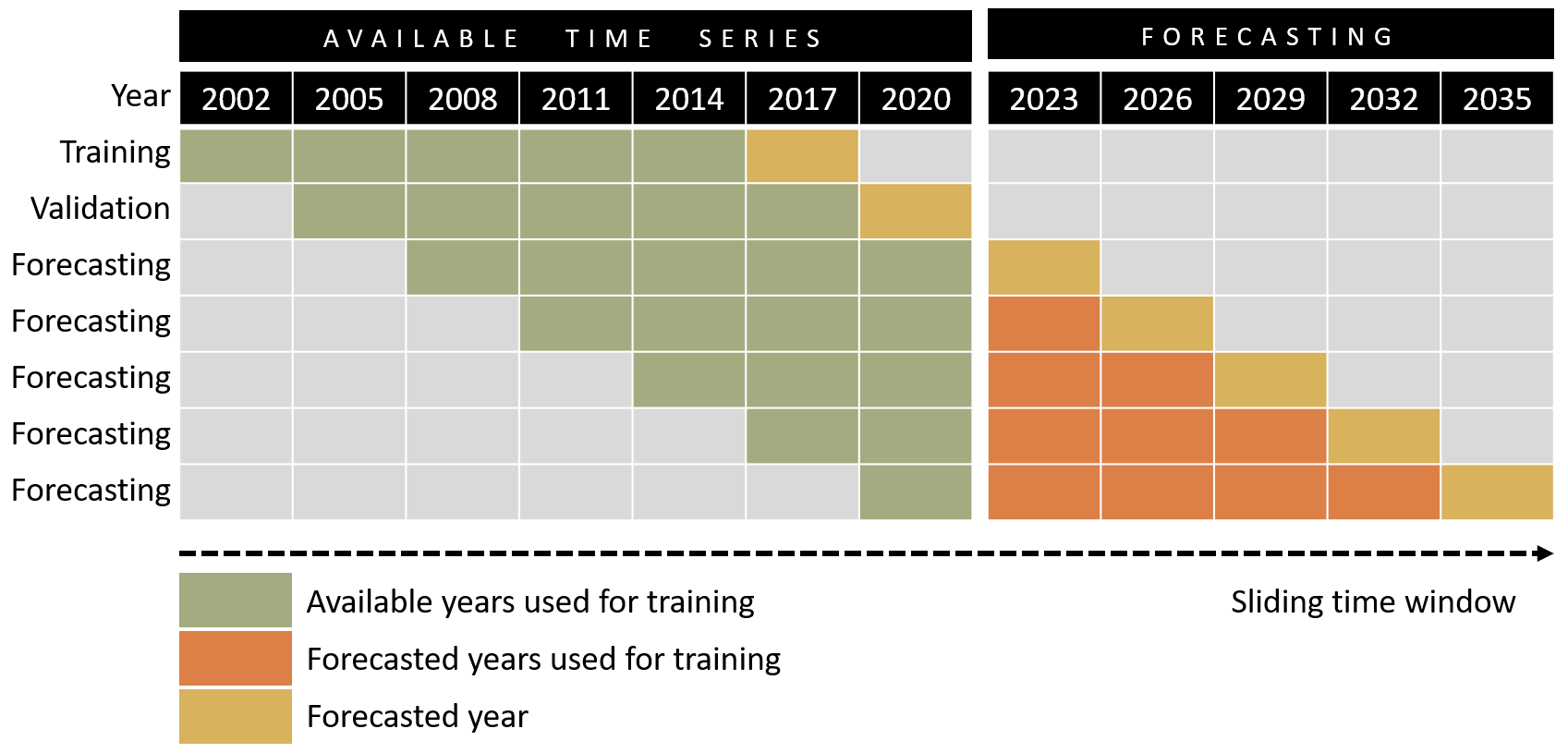
Figure 6 Forecasting concept; the training data set utilizes the earlier six time steps (e.g., 2002, 2005, …, 2017), whereas the validation data set utilizes the later six time steps (e.g., 2005, 2008, …, 2020) of the time series. We use the variables of the first five time steps as the input and the last time step as the ground truth labels. The aim of the training data set is to predict the population of the year 2017, and the aim of the validation data set is to forecast the population map for the year 2020. Forecasting beyond the year 2023 is obtained with a sliding time window strategy, where previous forecasted years are deployed for model training (adapted from Wang and Lee, 2021).

We carry out experiments with three sets of driving factors deployed for forecasting: (i) all driving factors described in Sect. 2.2; (ii) solely the time-invariant driving factors, i.e., slope, distances to bodies of water, roads, and the city center; and (iii) the population data only. Here it can be noted that the latter two reduced sets of variables enable the prediction of multiple time steps in the future. When also including time-variant driving factors, i.e., land cover and distance to the boundary of built-up areas, only one future time step can be predicted; a model learns the changes during a specific time interval and can thus predict the same time interval in the future. Equation (3) describes this relation:

$$\begin{array}{}\text{(3)}& t_{n+\mathrm{1}}=t_n+i,\end{array}$$

with t_n+1 being the forecasted year, t_n the year of the last input, and i the interval size. Here, we train all models with an interval i of 3 years including every third year as training data from the WorldPop time series data. To be more specific, if we input the years 2008, 2011, 2014, 2017, and 2020, the model is expected to produce an estimation for the year 2023. Subsequently, the year 2026 can be forecasted with the data of the year 2023 as input. The time-invariant driving factors can be assumed to be valid for 2023 too, and we predict the corresponding population data prior to that moment. In contrast, no valid estimates for 2023 are available regarding the time-variant driving factors. Thus, excluding the time-variant driving factors from the training enables iterative predictions of multiple intervals. We implement the sliding time window approach similarly to the forecasting strategy deployed by Wang and Lee (2021). A corresponding scheme is displayed in Fig. 6.

We train all the tested models for 50 epochs, using Adam as the optimizer and implementing mean-squared-error loss as the loss function, and set the initial learning rate to 0.0012. We reduce the learning rate by the factor 0.1 through a learning rate scheduler when the error reaches a minimum plateau. To evaluate the proposed framework, we adopt two baseline methods, i.e., MLR and RF. Thereby, we tune the hyperparameters of RF heuristically as follows: ntree = 500 and mtry = 1,2, …, 51.

4 Experimental results and discussion

4.1 Model evaluation

To provide a first comparative overview regarding prediction accuracy, Fig. 7 contains scatterplots of the different methods for the predicted year 2020. Thus, it illustrates the deviations in the forecasts (y axis) concerning the actual population values (x axis). Each point corresponds to one grid cell in the study area. The color coding reflects the point density in percentages, the red line is the regression line of forecasts and population values, and the black line corresponds to the identity line where y=x. It reveals that all models feature a substantial concentration of the density along the identity line, which underlines the overall validity of this study's setup. However, traceable differences regarding the different models exist. The majority of the baseline models based on linear regression and RF feature a lower point density along the identity line compared to the LSTM-based models, especially for grid cells with medium and high population values. The corresponding root-mean-squared error (RMSE) values also clearly indicate that the LSTM-based models outperform both the ConvLSTM models and the baseline methods. In detail, the uncertainty in terms of RMSE could be reduced from 4.298 (RF), 4.109 (MLR), and 3.946 (ConvLSTM, bidirectional), respectively, to 3.629 (LSTM, bidirectional) while maintaining an excellent model fit (R²= 0.995). Along this line of models, this corresponds to an increase of more than 14 % in terms of model accuracy.

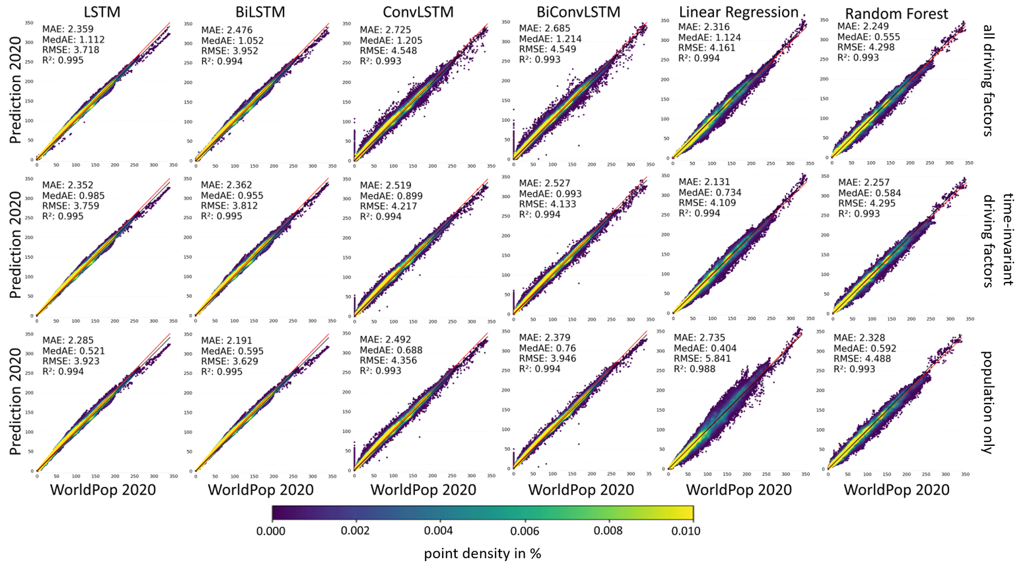
Figure 7 Scatterplots and corresponding error measures, i.e., mean absolute error (MAE), median absolute error (MedAE), root-mean-squared error (RMSE), and R², for the predicted year 2020 as a function of the actual prediction model, the learning mechanism, and the deployed driving factors.

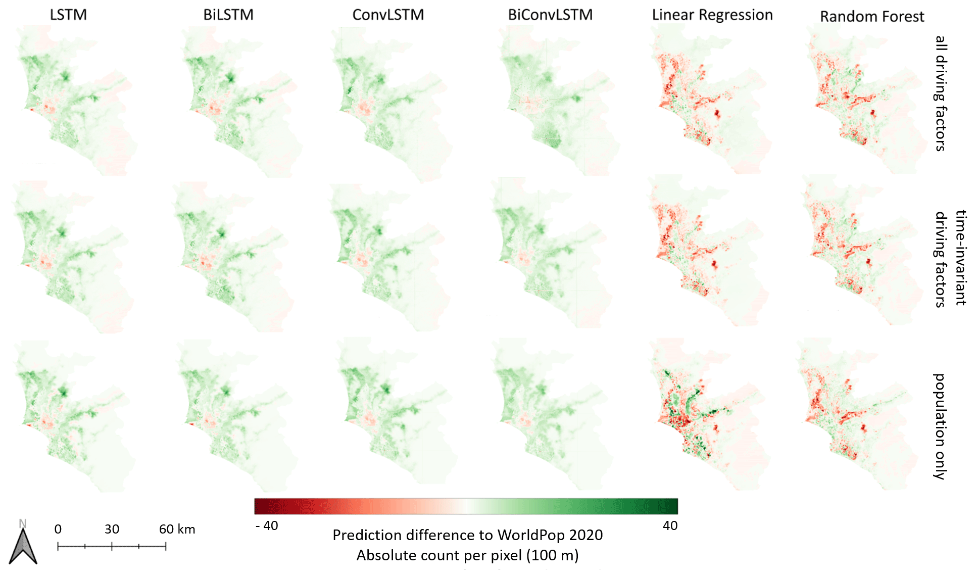
Figure 8 Maps of prediction differences in the models with respect to the actual numbers of 2020.

It can be noted that using the static features for the baseline models, i.e., MLR and RF, and solely deploying the population data for the LSTM and ConvLSTM with a bidirectional learning mechanism enabled the respective best predictions. Counterintuitively, the LSTM models outperform the ConvLSTM models unambiguously. Past works showed that the inclusion of additional spatial context information via ConvLSTMs can be beneficial for increasing prediction accuracy (Shi et al., 2015; Gavahi et al., 2021). However, in our idiosyncratic data setting, some inconsistencies in the WorldPop data can be found; bodies of water, conservation areas, or industry districts are traceably not masked during the disaggregation, which leads to mostly non-zero grid cell values in these areas. Solely the individual grid cells lying in these regions hold zero values in the WorldPop data. All convolutional models predict these grid cells with non-zero population, as they learn from the surrounding grid cells. This can be seen in Fig. 7 at x=0, where the actual population is zero, but the prediction differs quite strongly. Nevertheless, across all models, mean absolute error (MAE) values indicate a deviation of fewer than three people per grid cell, which stresses the overall soundness of this study's setup.

Figure 8 provides prediction differences from the actual numbers of 2020 from a spatial perspective. Grid cells with overestimated population numbers are colored in green, whereas grid cells with underestimated population numbers are colored in red. Thereby, it can be traced that the LSTM-based and ConvLSTM-based predictions overestimate population numbers for the majority of grid cells, while both the MLR-based and RF-based predictions underestimate population numbers for the majority of grid cells (also revealed by the regression line in Fig. 7). However, both the LSTM-based models and ConvLSTM-based models consistently follow the overall trend of area; they tend to exaggerate population numbers in areas of increasing population and underestimate population numbers in areas of decreasing population (see also Fig. 2 for a visualization of areas of increasing and decreasing population numbers in Lima and Callao). MLR-based and RF-based predictions do not reflect this overall trend, whereby overestimations and underestimations are more dispersedly distributed across the study area.

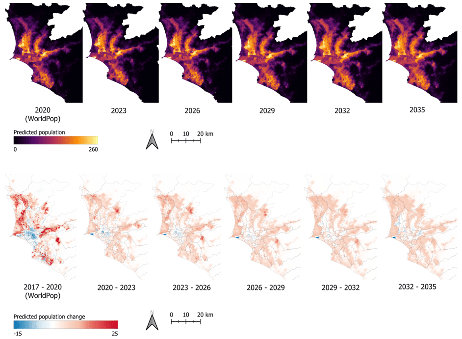
Figure 9 The upper row provides a visualization of the WorldPop data for the year 2020 and the forecasted population until the year 2035 on a 3-year interval. The lower row contains the corresponding predicted change in the population for the different time intervals.

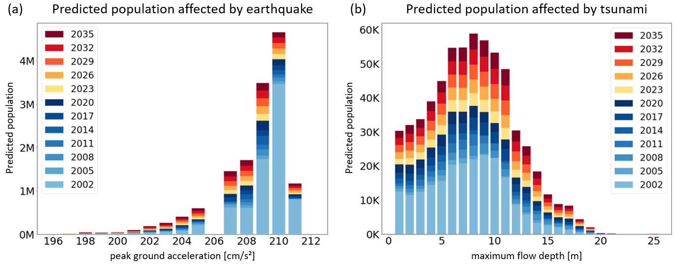
Figure 10 Predicted number of people affected by different hazard intensity levels on a 3-year interval (2002–2035) regarding (a) earthquakes and (b) tsunamis.

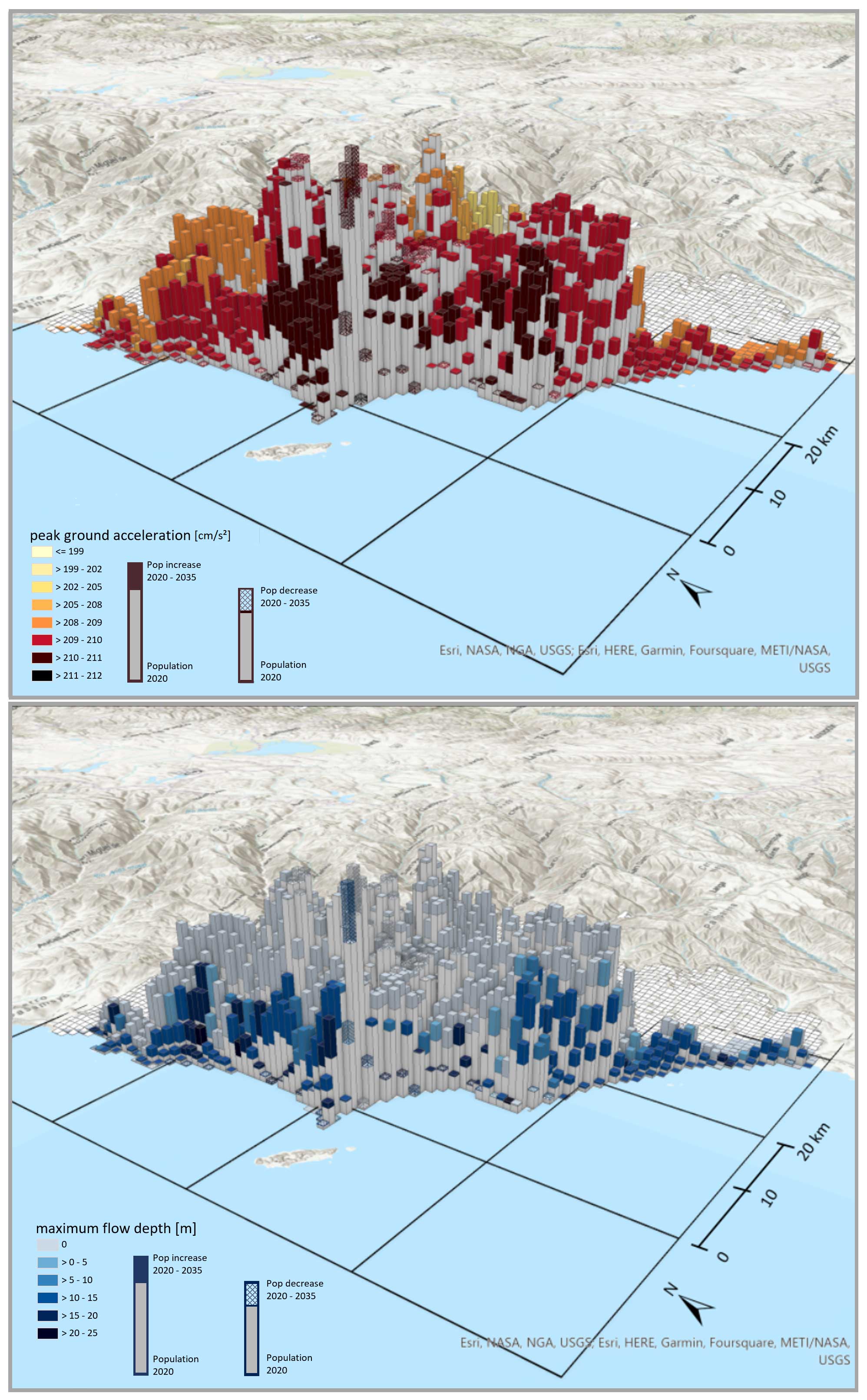
Figure 11 Maps of the predicted population affected by earthquakes (upper panel) and tsunamis (lower panel) for the year 2035 with corresponding hazard intensities. The solid grey bars indicate the population of the year 2020. The additional colored bar (on top) or textured bar indicates the estimated increase or decrease in the population until the year 2035, respectively. The corresponding color coding indicates the hazard intensity.

4.2 Population forecasting

We carry out the actual population forecasting, which is deployed for the subsequent exposure analysis, based on the most favorable model, i.e., the LSTM trained on the population data with a bidirectional learning mechanism. We implement this model in our forecasting concept (Fig. 6), where forecasting beyond the year 2023 is obtained with a sliding time window strategy; i.e., previously forecasted years are deployed for model training. Figure 9 displays both the forecasted population and the change between subsequent time steps until the year 2035. Thereby, the population increases by about 3.6 million, which accounts for 35 % of Lima's population in 2020.

4.3 Exposed future population

The hazard models (Sect. 2.4) and the predicted population distribution (Sect. 4.2) are employed to compute the future population count as a function of different hazard intensity levels. Figure 10 provides accumulated population numbers for different levels of peak ground acceleration (Fig. 10a) and maximum flow depth (Fig. 10b) along the 3-year time interval. It can be observed that the majority of the future population, i.e., 12.5 million inhabitants, lives in areas of high peak ground acceleration, i.e., PGA ≥ 207 cm s⁻². This number of future exposed population is induced by a growth of almost 30 % over the forecasted time span. This is lower than the 35 % growth in the whole Lima metropolitan area. However, more than 82 % of Lima's inhabitants reside in these districts today already. Consequently, this growth accounts for more than 70 % of the predicted additional people in Lima. Furthermore, more than 600 000 people are anticipated to live in areas which may face tsunami flow depths of 2 m or more. The population in the tsunami inundation area will grow by 61 % until 2035, much more than the average growth of 35 %. In the considered scenario, waves of up to 20 m are anticipated, and more than 430 000 people of the exposed population would be hit by waves higher than 5 m.

The forecasted spatial distribution of the population along with hazard intensities is visualized in Fig. 11 from a southwestern viewing angle. We aggregate the grid cells from the 100 m resolution to a 1 km resolution for visual representation. The visual inspection uncovers new future hot spots of the exposed population, i.e., areas that simultaneously face high population increases and severe hazard intensities, such as Lima and Callao's northwestern and southwestern settlement areas along the coastline. Anticipating those patterns can help urban planners and policymakers to proactively develop effective strategies for risk mitigation. For instance, the created information about exposed population can be part of modern decentralized information systems for (multi-)risk assessment (Schöpfer et al., 2023). Here, one core element is to enable end users to explore various scenarios (“stories”) of multiple hazards and cascading effects and their impacts by quantifying different “what-if” scenarios. Utilizing such a narrative-driven methodology empowers individuals to replicate diverse situations within a predetermined, multi-risk context, enabling them to assess and contrast outcomes. This multi-scenario approach proves invaluable for crafting strategies that fortify or enhance resilience, evaluating the effectiveness of proposed or already executed measures (e.g., benchmark scenarios) in the face of various hazard scenarios (acting as a “stress test”) or in response to evolving conditions. Thereby, the importance of implementing mechanisms to visualize epistemic and aleatory uncertainties about the risk assessment procedure in graphical form is stressed to allow appropriate communication with end users.

5 Conclusions and outlook

In this paper, we encode population-related geospatial change trajectories over time in an ML model and provide population forecasts for Peru's capital Lima and Callao to identify future hot spots of earthquake and tsunami exposure. The experimental results underline the superior performance of temporal models, i.e., LSTM-based networks, in accurate forecasting of the changes in population distribution. Given that the source data set with the tested data is openly accessible and has global coverage, our workflow can be generalized to forecast population changes in other locations with only a few adaptations (e.g., determine the best model hyperparameters empirically for a specific area/data set) for optimal forecasting accuracies.

Several extensions can be explored in future work. Foremost, it is crucial to obtain a picture of future risks and not solely of aspects of the exposure, i.e., the population at risk. This would require the collection of time series data for model training with multiple risk-related target variables including population, building types, and occupancies, among others, to also align vulnerability information, i.e., earthquake and tsunami-related fragility functions in order for a more thorough forecasting of future earthquake and tsunami risks to be conducted. From a methodological point of view, the consideration of multiple risk-related target variables also enables the development of multi-task learning models, which can encode interdependencies between the considered target variables to enhance the prediction accuracy (Geiß et al., 2022). Also, a multi-task model is able to learn the time-variant driving factors for enhanced forecasts and, thus, draw a more robust picture of future risks.