the Creative Commons Attribution 4.0 License.
the Creative Commons Attribution 4.0 License.
 | 03 Jan 2024
Slope Unit Maker (SUMak): an efficient and parameter-free algorithm for delineating slope units to improve landslide modeling
Jacob B. Woodard
Benjamin B. Mirus
Nathan J. Wood
Kate E. Allstadt
Benjamin A. Leshchinsky
Matthew M. Crawford
Slope units are terrain partitions bounded by drainage and divide lines. In landslide modeling, including susceptibility modeling and event-specific modeling of landslide occurrence, slope units provide several advantages over gridded units, such as better capturing terrain geometry, improved incorporation of geospatial landslide-occurrence data in different formats (e.g., point and polygon), and better accommodating the varying data accuracy and precision in landslide inventories. However, the use of slope units in regional (> 100 km2) landslide studies remains limited due, in part, to the large computational costs and/or poor reproducibility with current delineation methods. We introduce a computationally efficient algorithm for the parameter-free delineation of slope units that leverages tools from within TauDEM and GRASS, using an R interface. The algorithm uses geomorphic laws to define the appropriate scaling of the slope units representative of hillslope processes, avoiding the often ambiguous determination of slope unit size. We then demonstrate how slope units enable more robust regional-scale landslide susceptibility and event-specific landslide occurrence maps.
- Article
(9880 KB) - Full-text XML
-
Supplement
(6615 KB) - BibTeX
- EndNote


Landslides cause substantial losses of life, infrastructure, and property every year across the world (Froude and Petley, 2018). One of the most common tools for mitigating these losses is landslide-susceptibility mapping, which provides information on the spatial patterns and likelihood of landslide occurrence. Data-driven statistical models are typically used for creating these maps due to their computational efficiency and the relative availability of data needed to develop and deploy these models (van Westen et al., 2008). Statistical models analyze the spatial distribution of known landslides in relation to local terrain conditions (e.g., slope, curvature, aspect), and other areas with similar conditions are identified as being susceptible to landslides. In essence, the models identify features in the terrain similar to known landslides as a measure of landslide susceptibility. As such, the quality of the landslide inventory used to develop the susceptibility model is paramount for creating reliable maps. However, inventories with accurate information on landslide positioning, extent, triggering mechanism, and type are unavailable in many parts of the world. More often, if an inventory exists at all, it consists of a compilation of landslide data collected at different scales, times, accuracies, and formats (e.g., polygons or points) with limited information on the landslide type or triggering mechanism (Mirus et al., 2020).
Another tool used to mitigate losses associated with landslides are near-real-time or forecasted landslide occurrence models (Nowicki Jessee et al., 2018; Nowicki et al., 2014; Tanyas et al., 2019; Kirschbaum and Stanley, 2018). Rather than characterizing the potential of landslide existence from static terrain conditions, these models include a dynamic input designed to characterize landslide potential from a particular forcing event. For example, Tanyas et al. (2019) analyzed the static terrain conditions and dynamic ground motion metrics (e.g., peak ground velocity) from 25 earthquake-induced landslide-event inventories from across the world to create a landslide model that can estimate the distribution of landslides during an earthquake. Herein, we will refer to this model type as a landslide occurrence model. Like susceptibility models, landslide occurrence models often suffer from imperfect and heterogeneous landslide data. Thus, a common problem in the landslide community is determining an effective way of assessing landslide susceptibility and/or occurrence, despite the imperfect data available for model development.
The foundation of any landslide map (susceptibility and occurrence) is the mapping unit used to subdivide the terrain for landslide analysis. Grid cells (pixels) are the most used mapping unit, constituting about 86 % of all publications on landslide susceptibility as of 2018 (Reichenbach et al., 2018). This is due largely to their ease in processing. However, grid-based mapping units have several major drawbacks. First, the grid cells have no physical relationship to landslide processes. Landslides occur at various spatial scales and manifest a large range of footprints not appropriately captured by grid cells. Second, variable scales of data that describe the local terrain conditions used to develop landslide models (i.e., predictors or covariates) can lead to model biases. For example, the size of the grid cell can have major effects on the output of the landslide model (Chang et al., 2019; Guzzetti et al., 1999; Catani et al., 2013). To mitigate these effects, some researchers suggest creating multiple models at different resolutions (e.g., Guzzetti et al., 1999). Third, landslide inventories are often mapped using a mix of formats (i.e., polygon and points). This requires modelers to standardize the data in some way (Zêzere et al., 2017; Jacobs et al., 2020; Süzen and Doyuran, 2004; Zhu et al., 2017; Tanyas et al., 2019). For regional-scale (> 100 km2) models that use high-resolution (< 100 m) rasters, this standardization is often implemented by sampling a single representative cell from within each landslide polygon (Qi et al., 2010; Gorum et al., 2011; Xu et al., 2014; Oliveira et al., 2015). Alternatively, some studies use lower-resolution rasters (> 100 m) and sample all the cells that touch a landslide polygon or point (e.g., Nowicki et al., 2014).
Slope units alleviate many of the problems of grid mapping units and are based on drainage and divide lines that effectively segregate the terrain according to the hillslope processes that shaped it (Carrara, 1983; Guzzetti et al., 1999). First, the slope units' relationship with the natural terrain allows modelers to use an array of statistics of the predictors inside of the mapping unit (e.g., max, min, standard deviation). Second, the amalgamation of grid cells to create a slope unit provides a natural subset of the terrain that reduces the need for multiple raster resolutions for the susceptibility analysis (Jacobs et al., 2020). Third, slope units provide an alternative solution for the incorporation of landslide data in different formats. In contrast to the common grid-based standardization procedures, slope units allow modelers to study the characteristics of the whole hillslope(s) that experienced a landslide. Fourth, slope units are less sensitive to the effects of inaccurate landslide locations (Jacobs et al., 2020). Finally, although the use of slope units requires more processing at the beginning of the analysis, the limited number of mapping units enables the use of input data from every mapping unit, even over large regions. The representation of every mapping unit in the study area prevents the potential of sampling bias common when using grid mapping units (e.g., Oommen et al., 2011; Petschko et al., 2014).
Recognition of the advantages of slope units has led to many different methods for delineating them. However, the disadvantages of these methods include inhibiting computational costs, time-intensive manual cleaning and/or delineation, or indeterminate parameterizations that control the slope units' scaling. For example, the most rudimentary method for creating slope units is using watersheds to draw their boundaries (Carrara, 1988). A drawback of this approach is that the sizes of the slope units are determined by the user and difficult to reproduce. Additionally, the cleaning of artifacts, which occur during the watershed delineation process, can be highly labor-intensive. Computer-vision techniques (e.g., landform classification) have also been used to delineate slope units (Luo and Liu, 2018; Martinello et al., 2022; Zhao et al., 2012; Cheng and Zhou, 2018), which overcome the reproducibility and labor issues of the manual delineation method. However, the scale of the slope units is still often arbitrarily set. The algorithm r.slopeunits developed by Alvioli et al. (2020, 2016) uses watershed delineations whose shape and dimensions are determined by the user or an iterative optimization procedure (i.e., a parameter sweep) that evaluates the algorithm's outputs while using different input parameter values (see Alvioli et al., 2020, for details). Although the algorithm can avoid manual parameter assignments (i.e., parameter free), the computational expense of the parameter sweep can be prohibitive for large areas. For example, Alvioli et al. (2020) summarize a 3-month process to delineate slope units based on a 25 m digital elevation model (DEM) for the country of Italy while omitting the flat regions (∼24 % of the total area) using a 64-core machine with 320 GB of memory. Additionally, the optimization procedure required for the parameter-free delineation of slope units is not openly available. The limitations of all the current slope unit delineation methods prevent the widespread use of slope units in susceptibility modeling.
The scaling of slope units should not be arbitrarily set to avoid the modifiable areal unit problem (MAUP) (Openshaw and Taylor, 1983; Buzzelli, 2020; Goodchild, 2011). The MAUP occurs when the cartographic representation of data varies significantly by the scale of the mapping unit used to represent the data. MAUP is a challenging issue to overcome; however, determining a scale of the slope units so that they effectively capture the hillslope processes that lead to landslides can greatly mitigate the negative effects of the MAUP (Buzzelli, 2020). Alvioli et al. (2020) recognized this challenge, which motivated the development of their custom optimization procedure. Importantly, the optimal scale for capturing hillslope processes is spatially variant. Thus, the ideal scaling of slope units should adjust to the local topography.
The objective of this paper is to introduce Slope Unit Maker (SUMak), an open-source, slope-unit delineation tool that is computationally efficient and parameter-free, and to demonstrate how slope-unit-based landslide maps are generally a better mapping unit for regional (> 100 km2) landslide analysis. SUMak leverages the watershed optimization algorithm available in the software package “Terrain Analysis Using Digital Elevation Models” (TauDEM) (Tarboton, 2015) to determine the optimal scale of the watersheds for capturing hillslope processes. This optimization avoids the computationally inefficient parameter sweeps required by other parameter-free algorithms, making it markedly faster. To demonstrate the utility of SUMak, we divide this article into two parts: (1) an explanation and demonstration of our slope unit delineation algorithm and (2) an example of how slope units are generally a better mapping unit for regional landslide modeling due to the larger mapping units that align with the local terrain. In part two, we first show that slope units provide a conservative means of displaying the nebulous susceptibility model output caused by imprecise input data (e.g., no time component, imprecise locations, and/or variable formats). We do this by comparing landslide susceptibility map outputs from grid and slope-unit-based maps in two watersheds in the state of Oregon (USA) which have inventory data mapped at a range of scales and formats. Next, we demonstrate the advantages of slope units for assessing event-based landslide occurrence using a landslide catalog from Hurricane Maria over the island of Puerto Rico (Hughes et al., 2019). Landslide models are developed using logistic regression and XGBoost machine learning algorithms.
2.1 Slope unit delineation
To efficiently map slope units over a given terrain, we adapt tools from the software TauDEM (Tarboton, 2015) which determine the scale where the topography transitions from fluvial to hillslope processes using the constant drop law (Supplement Fig. S1). The constant drop law states that the average drop in elevation along Strahler stream orders (Strahler, 1957) is constant (i.e., independent of order) at scales, or aerial extents, of the terrain controlled by fluvial processes. At sufficiently small scales, the constant drop law does not hold, indicating that hillslope processes are controlling the terrain morphology. The scale at which the constant drop law breaks is determined by applying a series of flow accumulation thresholds to the input DEM and finding the threshold where the mean stream drop of the first-order streams is statistically different from the higher-order streams, using a T test (Davis, 2002). The stream accumulation threshold just below where the law breaks is then used to delineate the largest watersheds that capture the hillslope processes of that terrain. This scaling law is independent of the raster resolution (Tarboton et al., 1991; Tarboton, 1989) and has been used extensively in the field of fluvial geomorphology. We further process these optimally scaled watersheds by splitting them by the longest flow path within the watershed using GRASS (GRASS Development Team, 2020). Thus, the watersheds essentially become what would be objectively recognized as a slope. We argue that basing the scaling of slope units used for landslide analysis on established geomorphic laws provides the best justification for their appropriate sizing and odds of mitigating the negative effects of the MAUP.
If the domain of interest has significant variation in topography, TauDEM may choose a threshold that does not adequately characterize every area within the domain. Thus, SUMak provides different options for subdividing the domain in preparation for the application of the slope unit optimization procedure described above. We refer to these preliminary subdivisions as intermediate watersheds. Intermediate watersheds must be small enough to limit the variation in topography but large enough to avoid significantly reducing computational efficiency. While experimenting with different watershed dimensions on the topographically diverse regions of Sicily, Puerto Rico, and the Umpqua and Calapooia watersheds, we found an accumulation threshold of ∼100 km2 to adequately strike this balance. This threshold can be adjusted to meet the user's needs, or SUMak has an option to input predetermined intermediate watersheds. After appropriate intermediate watersheds are created, the algorithm runs the rest of the processing steps individually for each intermediate watershed in parallel as detailed in Sect. S1 and the online repository (Woodard, 2023).
2.2 Susceptibility maps
Several papers have evaluated the relative effectiveness of slope units over grid mapping units in statistical landslide susceptibility models (Jacobs et al., 2020; Steger et al., 2017; Zêzere et al., 2017; Van Den Eeckhaut et al., 2009; Martinello et al., 2022). However, none of these studies has thoroughly evaluated the effectiveness of slope units for better visualizing the imprecise susceptibility model outputs caused by inconsistent input data or their advantages in displaying near real-time or forecasted landslide occurrence maps. To demonstrate these benefits, we use the Middle Umpqua and Calapooia 10-digit hydrologic unit code (HUC) watersheds (U.S. Geological Survey, 2004) in the state of Oregon (USA) and the island of Puerto Rico, which have areas of 257, 743, and 8870 km2, respectively. Each area's landslide catalog includes an assortment of landslide types (slumps, debris flows, rockfalls, deep-seated landslides, and others), which are not differentiated in this study. The landslide data from Oregon were collected over decades using a combination of 1 m DEM data and their derivatives, geologic maps, orthophotos, aerial photography, and field reconnaissance and consist of both point and polygon data (Burns and Madin, 2009). The Oregon landslide catalogs contain no temporal constraints on landslide occurrence. The Umpqua dataset contains 941 points and 3213 polygons, while the Calapooia dataset contains 33 points and 456 polygons. In this dataset, polygons cover the extent of the landslide-affected area, while points are placed at the centroid of the landslide-affected areas. All data were reviewed for accuracy after their initial mapping. The areas of the individual landslides mapped using polygons are highly variable, spanning 30–4.4×10⁶ and 1500–1.88×10⁷ m2 in Umpqua and Calapooia, respectively. This data variability can lead to problems when using grid mapping units because the landslide data are standardized to a consistent format for the creation of the landslide susceptibility models. The Puerto Rico landslide dataset consists of 71 431 point locations of the centers of landslide headscarps that occurred during Hurricane Maria on 20–21 September 2017 (Hughes et al., 2019). Headscarps were manually identified using high-resolution (15–50 cm), post-event imagery and quality checked by three experienced supervisors. Importantly, the output of the landslide models for Puerto Rico is not a susceptibility map, rather a landslide occurrence map. That is, the models output the probability of a landslide occurring during Hurricane Maria. This type of output is similar to the landslide models developed for near-real-time or forecasted assessment of event-specific landslides (Nowicki Jessee et al., 2018; Nowicki et al., 2014; Tanyas et al., 2019; Kirschbaum and Stanley, 2018). Our example from Hurricane Maria is intended to show how event-specific model outputs might differ between slope unit and pixel-based assessments. Thus, the Oregon watersheds and Puerto Rico datasets are used to demonstrate the benefits of slope units when using inconsistent and event-based input data, respectively.
We evaluate four different methods of standardizing landslide polygons to points for grid-based susceptibility maps in the Oregon watersheds. Each method converts the polygons to points which are combined with the landslides originally mapped as points. The first method converts the landslide polygons into a single point at the highest elevation cell within the polygon using a 10 m DEM from the U.S. Geological Survey's three-dimensional (3D) Elevation Program (3DEP) database (U.S. Geological Survey, 2019), which has a vertical root mean square error of 0.82 m (Stoker and Miller, 2022). In cases where there are multiple points, the highest elevation cell with the highest slope is selected. This sampling method is designed to capture the attributes nearest the landslide scarp and the conditions that led to failure (Zêzere et al., 2017; Süzen and Doyuran, 2004; Jacobs et al., 2020). The second method follows the same procedure but is conducted using the same 10 m DEM resampled to 30 m resolution using a bilinear interpolation method. The coarser raster may better average the landslide characteristics compared to the finer-resolution rasters. Third, we sample multiple random points from the 10 m DEM within the polygons with a 200 m spacing, roughly halfway between the average radii of the landslide polygons from the two study sites (93 and 386 m for Umpqua and Calapooia, respectively). Each landslide polygon is guaranteed at least one point. Creating multiple points within the polygons allows us to capture some of the variability in the large landslides' measured attributes without eliminating the influence of landslides originally mapped as points. Using all the raster cells within the polygons would oversaturate the model with data from the landslide polygons and greatly reduce the influence of the landslides originally mapped as points due to their relative sparsity. Finally, we sample a point within each polygon at the median elevation value using the 10 m DEM. In the case of multiple points per polygon, we select the point with the highest slope. This dataset is used to verify that the chosen statistics in the slope-unit-based approach did not bias the results and to make the standardization more compatible with the Oregon point data. We refer to these four sampling methods as “10m”, “30m”, “10m_multi”, and “10m_med”, respectively. For the Puerto Rico dataset, we only use the “30m” sampling method as this dataset is used to demonstrate the use of slope units for event-based landslide inventories rather than inconsistent inventories. For all study sites, non-landslide data are randomly sampled from areas outside the landslide polygons and points buffered with a radius derived from the average area of the landslide polygons within each study area. For Puerto Rico, this radius is set to a value between the two Oregon mean polygon radii (100 m). If a landslide originally mapped as a point is within the boundaries of a landslide polygon, it is removed before standardization. The sampling ratio of landslide and non-landslide points is set to 1:1, following the most common practice (Petschko et al., 2014; Reichenbach et al., 2018). Table S1 shows the number of points for each study site and sampling method, respectively.
Slope units for the study sites are delineated using the same 10 m DEM as the grid-based approaches. We note that slope units can be delineated with coarser-resolution elevation data with a loss in precision. The sampling scheme for the slope-unit-based maps is simpler than the grid-based schemes. Each slope unit in the study area is set to be either a landslide sample or non-landslide sample dependent upon the intersection of a landslide point or polygon within that slope unit. We use an overlap threshold of 0.1 % (i.e., at least 0.1 % of the slope unit is covered by a landslide polygon) for determining the positive presence of landslides within a given slope unit (Jacobs et al., 2020). Figures S2–S3 illustrate the slope units that contain landslides. In the Umpqua, Calapooia, and Puerto Rico study sites, 68 %, 28 %, and 4 % of the slope units contained landslides, respectively. For the slope-unit-based maps, we train two different models. The first uses only the median value of the predictor data within the slope unit, and the other uses the median and standard deviation (SD) of the predictor data. To assure that the sampling ratio does not bias the comparison between the slope-unit- and grid-based maps, we set the sampling ratio of landslide and non-landslide locations to 1:1 for the slope unit maps.
We created landslide susceptibility models using the logistic regression and XGBoost (Chen and Guestrin, 2016) machine learning algorithms. Logistic regression is the most commonly used algorithm for data-driven landslide susceptibility modeling (Reichenbach et al., 2018). It calculates the log odds (, where P is the probability), of a binary outcome given some predictor data (x) that describe the terrain. For M input predictors, logistic regression is expressed as follows:
The input data's coefficients (β) are fit to the input data using a maximum likelihood criterion. XGBoost (https://xgboost.readthedocs.io/, last access: 20 December 2023) uses a gradient boosting decision tree algorithm that increases in complexity until the lowest model residuals are reached (Chen and Guestrin, 2016). This algorithm is fast, is easy to implement, and has been shown to produce highly accurate susceptibility maps (Sahin, 2020). To increase the model accuracy while preventing overfitting, we optimize the “max_depth”, “min_child_weight”, “subsample”, “gamma”, and “colsample_bytree” hyperparameters of XGBoost (see Sect. S2 for an explanation of these parameters) using a Bayesian cross-validation procedure. In short, these hyperparameters adjust how the model adapts to fit the training data. The Bayesian cross-validation procedure uses 10 folds and 10 iterations and assesses the results from the previous iterations to inform the next iteration of hyperparameters to use (Snoek et al., 2012). This procedure prevents the use of unwieldly grid searches and permits faster optimization of the model hyperparameters. For both algorithms, we limit the predictor variables to elevation, slope, aspect (ϕ), roughness (standard deviation of the elevation using a 100 m square window), and curvature to illustrate the effectiveness of the different models using only widely available data. Aspect is measured using to make it periodic and to account for variations in solar heat flux (McCune and Keon, 2002). As the Puerto Rico landslide dataset has a known trigger, we also include root zone soil moisture estimates from NASA's Soil Moisture Active Passive (SMAP) mission on 21 September 2017. Bessette-Kirton et al. (2019) found the SMAP data to be a better predictor of landslide distributions from Hurricane Maria than other rainfall datasets. After the models are trained, we generated maps by applying the trained models to the entire study areas.
Importantly, the meaning of the models' output probability is different depending on the sampling methods used. The single-cell methods (“10m”, “30m”, “10m_med”) measure the probability of a cell containing the high point (scarp) or center point of a landslide deposit recognized by the team(s) that compiled the landslide inventory. The multiple cell method (“10m_multi”) measures the probability of a cell containing a landslide deposit recognized by the team(s) that compiled the landslide inventory. Lastly, the slope-unit-based maps measure the probability of a slope unit containing a landslide recognized by the team(s) that compiled the inventory. For the two Oregon watersheds, the probability output of each method is used as a measure of landslide susceptibility. In contrast, the Puerto Rico maps output the probability of landslide occurrence during Hurricane Maria.
We measure the accuracy of the landslide models using the area under the curve (AUC) of the receiver operator characteristics (ROC) and the Brier score (Brier, 1950). The ROC curve compares the true positive rate against the false-positive rate at various discrimination thresholds (see Oommen et al., 2011, for an overview). If every landslide and non-landslide from the data is modeled correctly, the AUC values of the ROC curve will be 1.0. In contrast, AUC values near 0.5 suggest the model classification is equivalent to random guessing. Values from 0.5–0.6, 0.6–0.7, 0.7–0.8, 0.8–0.9, and 0.9–1.0 can be classified as poor, average, good, very good, and excellent performance, respectively (Yesilnacar, 2005). The Brier score (B) measures the mean-square error between the model predictions (i.e., probability, P) and observations (binary variable of landslide presence, O):
where N is the number of observations (Brier, 1950). Thus, a B value of zero suggests perfect model fit, and a value of 1 indicates perfect misfit. In contrast to AUC–ROC, the Brier score provides a measure of the scale of the model fit and not just its ordering of landslide and non-landslide observations. Both metrics together provide a comprehensive evaluation of the model results. Following common practice (e.g., Molinaro et al., 2005), we use 70 % of the data to perform a 10-fold cross-validation procedure with 10 iterations to optimize the models parameters and obtain representative distributions of the ROC–AUC and Brier score metrics while reserving 30 % of the data as a final test set. Model development and post-processing is conducted within R (R Core Team, 2022).
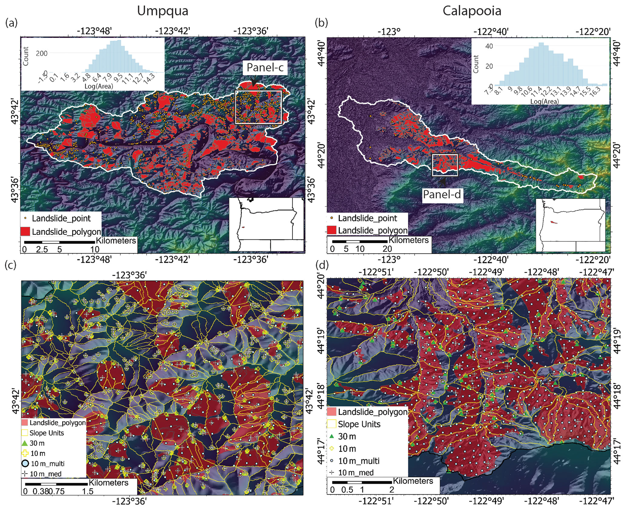
Figure 1Umpqua and Calapooia watersheds in Oregon. (a, b) Digital elevation models and landslide inventories. Also shown are the log-normalized histograms of the landslide polygon areas. (c, d) Zoomed-in portions of the slope unit maps with landslide polygons and grid-sampled points using the four sampling techniques superimposed. The 10 m point samples often overlap the 30 m samples. Sampling techniques are described in Sect. 2.2.
3.1 SUMak slope unit delineation
SUMak quickly delineates slope units over the three study areas while automatically adapting the scaling of the slope units by the local terrain. Table 1 shows the time to delineate each of the study areas. Both Oregon watersheds were delineated in only a few minutes, while the island of Puerto Rico took substantially longer. This is due to the larger area and the increased complexity of the delineating watersheds near coastlines where watersheds get increasingly small due to decreased accumulation areas. The adaptation of the slope unit sizes to the local topography is apparent in the slope unit maps (Figs. S4, 1–2). For example, the Calapooia Watershed includes a mountainous and flat region (Fig. 1). SUMak creates smaller slope units over the flat region compared to the mountainous region to accommodate the difference in scale where hillslope processes occur (Fig. S4).
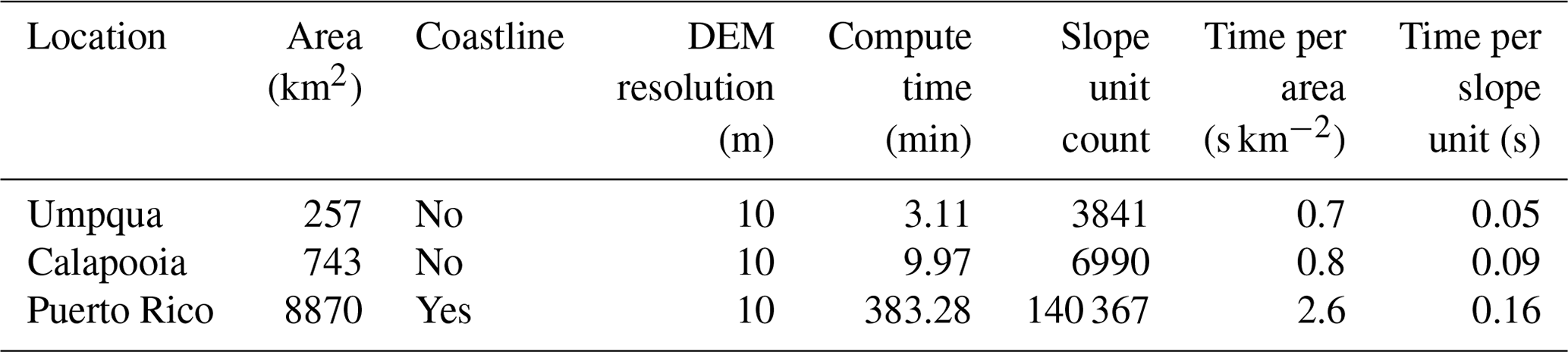
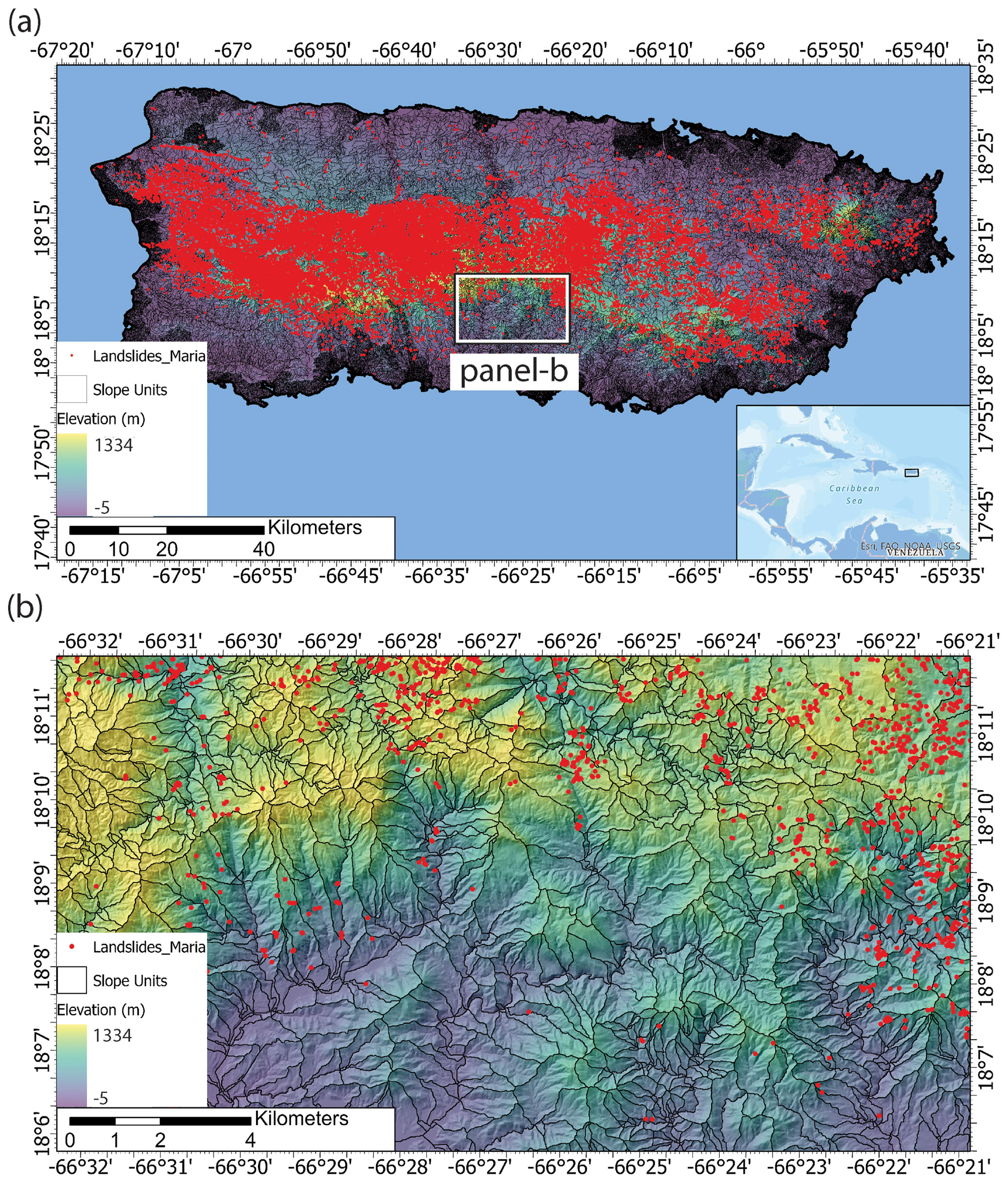
Figure 2Island of Puerto Rico. (a) Slope unit delineation and mapped landslide points from Hurricane Maria. (b) Zoomed-in portion of the island. Basemap from Esri's World Topographic Map (Esri, 2021).
3.2 Landslide map comparison
Comparison of the final landslide maps to the distribution of landslide deposits highlights several differences between the grid and slope-unit-based maps. The landslide inventories and examples of the grid sampling methods for the Oregon watersheds and Puerto Rico are in Figs. 1 and 2, respectively. The slope units provide a division for landslides that enables the characterization of the entire slope(s) that experiences a failure (Figs. 1c, d, 2). In contrast, the grid-based methods either minimize the entire landslide to a single representative point even for large (> 1 km2) landslides or an array of points. Figures 3 and 4 show the final landslide maps of the Oregon watersheds and Puerto Rico, respectively, using the 30 m sampling method for the grid-based maps and the slope-unit-based maps using the median and SD predictor values with XGBoost. The other landslide maps are in Figs. S5–S10. The slope unit maps generally better distinguish high and low probability zones with less area displaying probabilities near 0.5. Cumulative distribution functions of the maps' probabilities are shown in Figs. S11 and S12. Additionally, the slope-unit-based maps are more granular, which prevents the more localized variation in probability present in the grid-based maps. This granularity generally results in a higher percent of study sites' areas displaying higher probabilities (Figs. S13–S14). We note that the difference in map granularity is less for Puerto Rico than for the Oregon watersheds, likely due to the scale of mapped area, 30 m mapping unit, and the density of the landslide points (Fig. 2). Finally, the different maps highlight similar locations within the watersheds as having a relatively high or low probabilities.
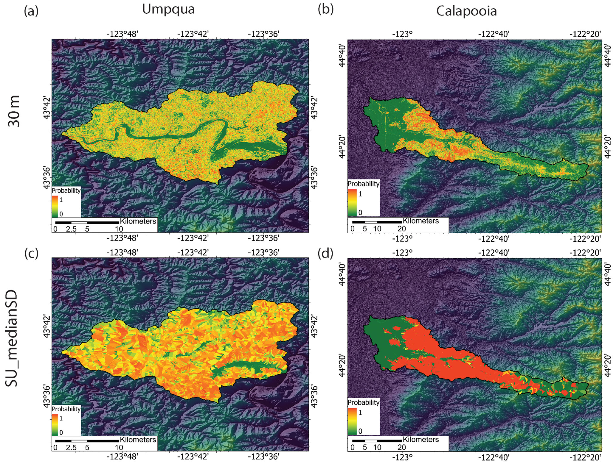
Figure 3Landslide susceptibility models for the Umpqua and Calapooia watersheds using (a, b) the 30 m sampling method for the grid-based maps and (c, d) slope units with median and standard deviation predictor values (SU_medianSD) with XGBoost.
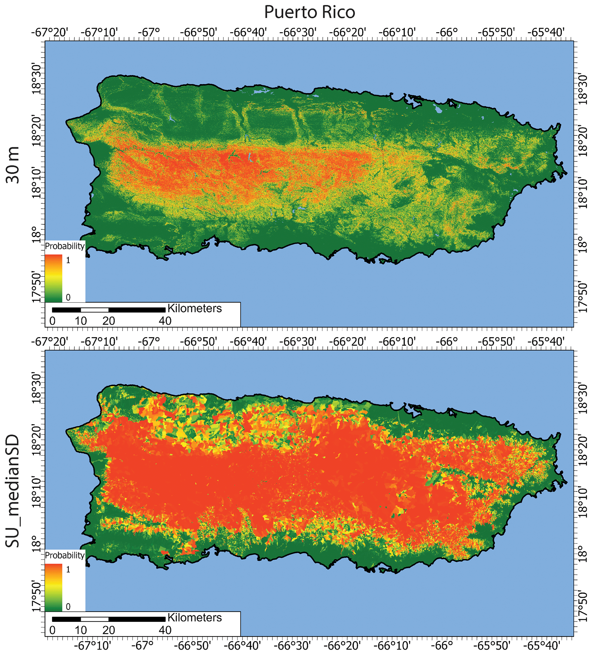
Figure 4Puerto Rico landslide occurrence models from the 30 m grid-based maps and using slope units with median and standard deviation predictor values (SU_medianSD) with XGBoost.
Both the ROC–AUC and Brier score metrics show a better model fit using slope units compared to any of the grid-based models for our study sites (Figs. 5 and 6). The XGBoost and logistic regression machine learning algorithms show an increase in the median ROC–AUC and a decrease in the Brier scores for the slope-unit-based maps. For example, at Calapooia, the XGBoost algorithm on the grid-based models showed AUC–ROC values that would qualify as very good model performance (average of 0.83) when applied to the test data, while the two final slope-unit-based models had excellent performance (average of 0.96) when applied to the test data. The Brier scores of the same models applied to the test data demonstrate an average mean-square error of 0.17 and 0.07 for the grid-based and slope unit models, respectively. Using the median and SD of the predictor values in each slope unit also increases the model performance compared to slope unit models developed with only the median predictor values. The different sampling techniques for the grid-based maps showed little variation in the two model performance metrics. Finally, XGBoost generally shows better model performance compared to logistic regression. In summary, the slope-unit-based models can better differentiate high and low probability areas of the terrain.
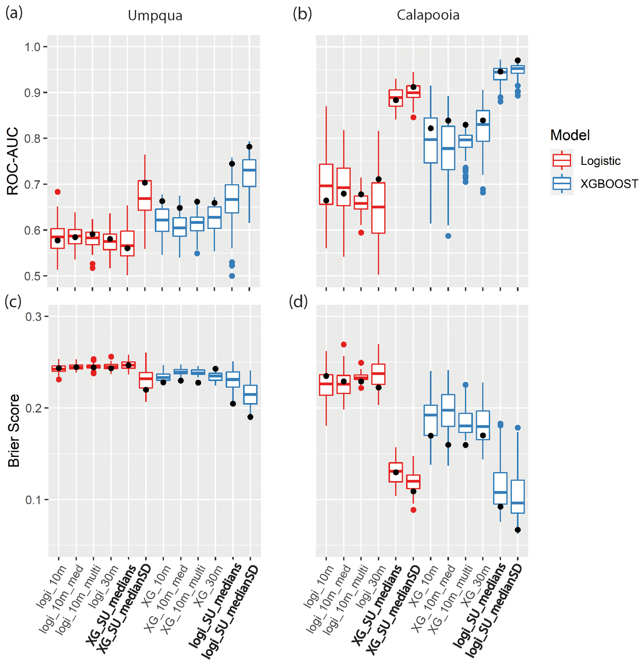
Figure 5(a, b) Receiver operator characteristics (ROC) area under the curve (AUC) and (c, d) Brier score boxplots from the 10-fold cross-validation procedure for landslide susceptibility models using the XGBoost (blue) and logistic regression (red) machine learning algorithms. The box hinges show the first and third quartiles; the whiskers extend to a maximum of 1.5 times the inter-quartile range; the red and blue dots show the data outlying the whiskers; the horizonal bars show the median values of the distributions. Distributions are for the different sampling methods (10m, 30m, 10m_multi, 10m_med) and the slope unit (SU) maps using only the median (SU_medians) and the median and standard deviation of the predictor values (SU_medianSD). The black dots show the scores of the test datasets.
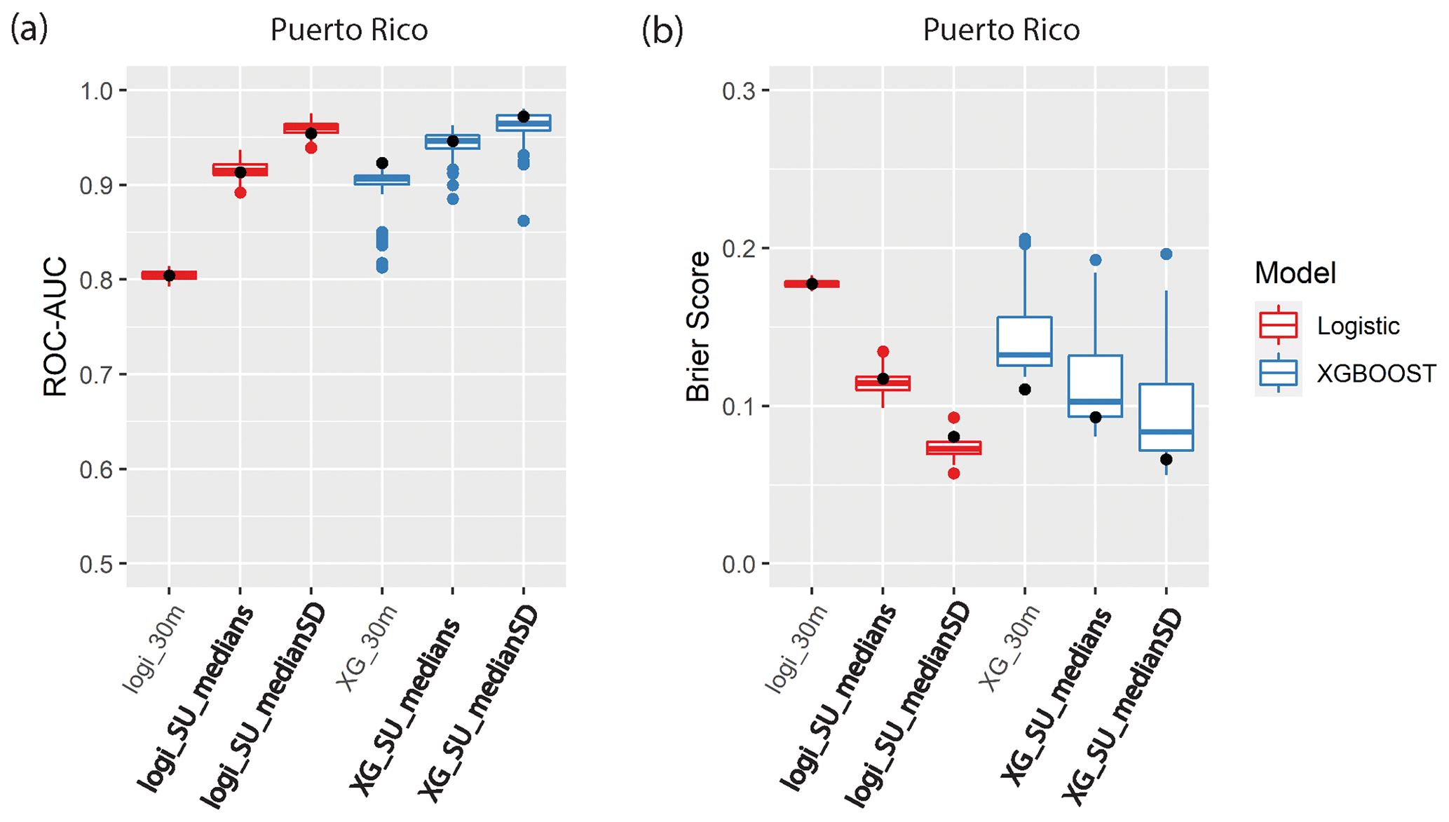
Figure 6(a) ROC–AUC and (b) Brier score boxplots from the 10-fold cross-validation procedure for landslide susceptibility models using the XGBoost (blue) and logistic regression (red) machine learning algorithms for the Hurricane Maria landslide catalog in Puerto Rico. Symbology is the same as Fig. 5.
Our slope unit delineation algorithm, SUMak, has significant advantages over previous delineation methods. In contrast to other methods which use an optimization function or user-dictated setting for determining the appropriate scaling and positions of slope units, SUMak uses established geomorphic laws for determining an appropriate scale of the slope units to capture hillslope processes. This scaling provides a non-arbitrary scaling of the slope units that are optimized to capture hillslope processes and help prevent MAUP. Lastly, SUMak is computationally efficient compared to some other parameter-free algorithms. These advantages, coupled with it being open-source and easy-to-use, make it desirable for an array of geomorphic analyses.
Our analysis highlights some of the benefits and drawbacks of using grids or slope units for landslide susceptibility modeling when using landslide data with variable formats and no temporal component. While both methods generally highlight the same areas as being more susceptible, the 30 and 10 m resolution grid mapping units used in this study produce maps with smaller scale variations in susceptibility. While this level of detail can be advantageous, the vague nature of the susceptibility models' output caused by imprecise input data (e.g., no time component, imprecise locations, and variable formats) generally used to make susceptibility maps can cause misleading results. Indeed, producing high-resolution (< 100 m) grid-based maps is attempting to output results beyond the capacity of the input data. For example, in the Umpqua watershed, all the grid-based maps show only half of the terrain as having higher (P > 0.5) susceptibility (Fig. S11). This phenomenon may partially reflect the limits of the statistical models used. However, slope units consistently produce more granular model results compared to grid-based maps independent of the model used, suggesting that the improved model performance is not merely an artifact of the statistical models. The lack of granularity of the grid-based maps at the Umpqua watershed may lead some to conclude that the watershed is generally not susceptible to landsliding. However, the abundance of the mapped landslides in the region (Fig. 1b) indicates that most of the Umpqua watershed is highly prone to landsliding. This shortcoming of the grid-based maps is also reflected in the poorer model metrics (Fig. 5). In contrast, the larger mapping units available through slope units allow for a more conservative map that, we argue, better captures the level of susceptibility, even with imprecise input data. This is supported by the better model metrics (Fig. 5) and a higher proportion of the Umpqua terrain as having higher susceptibility (Figs. 3, S11, and S12). More conservative grid-based maps are generally achieved using larger grid cells, which accentuates the unrealistic geometry of the cells and exacerbates the imprecise mapping of susceptible areas. Thus, slope units provide an effective mapping unit that accurately delineates the terrain into slopes that can be used to create conservative susceptibility maps that better accommodate the nebulous output of regional susceptibility models created with inconsistent input data.
Slope units also provide a more conservative output for event-based landslide occurrence maps that may be more effective at communicating the likelihood of landsliding over large regions for some use cases. Like the maps created using non-temporal landslide datasets, the grid-based occurrence maps created for Puerto Rico show fine-scale variations in landslide probability that may be outputting results at too fine a resolution for the input data used to develop the model. This resolution results in high spatial heterogeneity of probability values within a single hillslope. Figure S15 shows a zoomed-in portion of the model results and illustrates the diversity in probability values in the grid-based map compared to the slope unit map within a relatively small, mountainous terrain. The grid-based Puerto Rico landslide models are attempting to specify the pixel that contains the center of the head scarp. This level of precision may be useful for some purposes but can be misleading and cause the model to miss the location of landslides induced by Hurricane Maria. In contrast, the slope unit maps characterize the susceptibility of the entire hillslope and thus provide a more conservative output that better generalizes the location of hurricane-induced landslides. One tradeoff of using a larger mapping unit is that the model may assign the same high-probability value to the entirety of the slope unit even if landslides only affect a small portion of the slope unit. This can lead to maps that show larger areas as being more prone to landsliding compared to grid-based approaches; thus, slope units may not be appropriate for some landslide mitigation products.
Here we have focused on using slope units for statistical landslide susceptibility and near-real-time landslide prediction modeling; however, objectively divided terrain can be used in an array of geomorphic studies. For instance, slope units could improve other landslide studies such as physically based models, early warning systems, debris flow modeling, or hazard assessments. These studies often use grid-based analysis which suffers from some of the same drawbacks of grid-based susceptibility modeling. Thus, adopting slope units as the mapping unit for these studies could yield more favorable results. Slope units could also help downscale topographically sensitive measurements (e.g., soil moisture, land cover) and provide a reasonable mapping unit for hydrologic and avalanche studies. Thus, SUMak could facilitate advances in geospatial analysis across several research areas beyond landslide susceptibility analysis.
The widespread use of slope units as the mapping unit of choice in landslide studies has been limited partially due to the lack of an efficient and easy-to-use method for delineating them. Here we introduce a new parameter-free algorithm for the automatic delineation of slope units. The algorithm is relatively computationally efficient and can be implemented anywhere there are digital elevation data. We also demonstrate that landslide maps created with slope units are more accurate and conservative compared to grid-based approaches.
The code for SUMak and data used in this article are available at Woodard (2023, https://doi.org/10.5066/P98NXFTN).
The supplement related to this article is available online at: https://doi.org/10.5194/nhess-24-1-2024-supplement.
JBW developed the SUMak algorithm and drafted the paper. BBM, NJW, KEA, BAL, and MMC reviewed the manuscript and contributed to the interpretation of the results.
The contact author has declared that none of the authors has any competing interests.
Any use of trade, firm, or product names is for descriptive purposes only and does not imply endorsement by the U.S. Government.
Publisher’s note: Copernicus Publications remains neutral with regard to jurisdictional claims made in the text, published maps, institutional affiliations, or any other geographical representation in this paper. While Copernicus Publications makes every effort to include appropriate place names, the final responsibility lies with the authors.
We thank two anonymous reviews for their suggestions for improving the manuscript.
This paper was edited by Paola Reichenbach and reviewed by two anonymous referees.
Alvioli, M., Marchesini, I., Reichenbach, P., Rossi, M., Ardizzone, F., Fiorucci, F., and Guzzetti, F.: Automatic delineation of geomorphological slope units with r.slopeunits v1.0 and their optimization for landslide susceptibility modeling, Geosci. Model Dev., 9, 3975–3991, https://doi.org/10.5194/gmd-9-3975-2016, 2016.
Alvioli, M., Guzzetti, F., and Marchesini, I.: Parameter-free delineation of slope units and terrain subdivision of Italy, Geomorphology, 358, 107124, https://doi.org/10.1016/j.geomorph.2020.107124, 2020.
Bessette-Kirton, E. K., Cerovski-Darriau, C., Schulz, W. H., Coe, J. A., Kean, J. W., Godt, J. W., Thomas, M. A., and Stephen Hughes, K.: Landslides triggered by Hurricane Maria: Assessment of an extreme event in Puerto Rico, GSA Today, 29, 4–10, https://doi.org/10.1130/GSATG383A.1, 2019.
Brier, G. W.: Verification of Forecasts Expressed in Terms of Probability, Mon. Weather Rev., 78, 1–4, 1950.
Burns, W. J. and Madin, I. P.: Protocol for inventory mapping of landslide deposits from light detection and ranging (lidar) imagery, Oregon Dep. Geol. Miner. Ind., 42, 1–30, 2009.
Buzzelli, M.: Modifiable Areal Unit Problem, in: International Encyclopedia of Human Geography, edited by: Kobayashi, A., Elsevier, Amsterdam, the Netherlands, 169–173, https://doi.org/10.1016/B978-0-08-102295-5.10406-8, 2020.
Carrara, A.: Multivariate models for landslide hazard evaluation, J. Int. Assoc. Math. Geol., 15, 403–426, https://doi.org/10.1007/BF01031290, 1983.
Carrara, A.: Drainage and divide networks derived from high-fidelity digital terrain models, in: Quantitative analysis of mineral and energy resources, edited by: Chung, C. F., Fabbri, A. G., and Sinding-Larsen, R., D. Reidel Publishing Company, 581–597, https://doi.org/10.1007/978-94-009-4029-1_34, 1988.
Catani, F., Lagomarsino, D., Segoni, S., and Tofani, V.: Landslide susceptibility estimation by random forests technique: sensitivity and scaling issues, Nat. Hazards Earth Syst. Sci., 13, 2815–2831, https://doi.org/10.5194/nhess-13-2815-2013, 2013.
Chang, K. T., Merghadi, A., Yunus, A. P., Pham, B. T., and Dou, J.: Evaluating scale effects of topographic variables in landslide susceptibility models using GIS-based machine learning techniques, Sci. Rep., 9, 12296, https://doi.org/10.1038/s41598-019-48773-2, 2019.
Chen, T. and Guestrin, C.: XGBoost: A scalable tree boosting system, Proc. ACM SIGKDD Int. Conf. Knowl. Discov. Data Min., San Fransisco, California, 13–17 August, 785–794, https://doi.org/10.1145/2939672.2939785, 2016.
Cheng, L. and Zhou, B.: A new slope unit extraction method based on improved marked watershed, MATEC Web Conf., 232, 1–5, https://doi.org/10.1051/matecconf/201823204070, 2018.
Davis, J. C.: Statistics and Data Analysis in Geology, Third, edited by: Gerber, M., John Wiley & Sons, Inc., New York, NY, ISBN 978-0-471-17275-8, 2002.
Esri: World Topographic Map, https://www.arcgis.com/home/item.html?id=30e5fe3149c34df1ba922e6f5bbf808f (last access: 20 December 2023), 2021.
Froude, M. J. and Petley, D. N.: Global fatal landslide occurrence from 2004 to 2016, Nat. Hazards Earth Syst. Sci., 18, 2161–2181, https://doi.org/10.5194/nhess-18-2161-2018, 2018.
Goodchild, M. F.: Scale in GIS: An overview, Geomorphology, 130, 5–9, https://doi.org/10.1016/j.geomorph.2010.10.004, 2011.
Gorum, T., Fan, X., van Westen, C. J., Huang, R. Q., Xu, Q., Tang, C., and Wang, G.: Distribution pattern of earthquake-induced landslides triggered by the 12 May 2008 Wenchuan earthquake, Geomorphology, 133, 152–167, https://doi.org/10.1016/j.geomorph.2010.12.030, 2011.
GRASS Development Team: Geographic Resources Analysis Support System (GRASS) Software, Version 7.8, https://grass.osgeo.org (last access: 20 December 2023), 2020.
Guzzetti, F., Carrara, A., Cardinali, M., and Reichenbach, P.: Landslide hazard evaluation: a review of current techniques and their application in a multi-scale study, Central Italy, Geomorphology, 31, 181–216, https://doi.org/10.1016/S0169-555X(99)00078-1, 1999.
Hughes, K. S., Bayouth García, D., Martínez Milian, G. O., Schulz, W. H., and Baum, R. L.: Map of slope-failure locations in Puerto Rico after Hurricane María, https://doi.org/10.5066/P9BVMD74, 2019.
Jacobs, L., Kervyn, M., Reichenbach, P., Rossi, M., Marchesini, I., Alvioli, M., and Dewitte, O.: Regional susceptibility assessments with heterogeneous landslide information: Slope unit- vs. pixel-based approach, Geomorphology, 356, 107084, https://doi.org/10.1016/j.geomorph.2020.107084, 2020.
Kirschbaum, D. and Stanley, T.: Satellite-Based Assessment of Rainfall-Triggered Landslide Hazard for Situational Awareness, Earth's Future, 6, 505–523, https://doi.org/10.1002/2017EF000715, 2018.
Luo, W. and Liu, C. C.: Innovative landslide susceptibility mapping supported by geomorphon and geographical detector methods, Landslides, 15, 465–474, https://doi.org/10.1007/s10346-017-0893-9, 2018.
Martinello, C., Cappadonia, C., Conoscenti, C., and Rotigliano, E.: Landform classification: A high-performing mapping unit partitioning tool for landslide susceptibility assessment – a test in the Imera River basin (northern Sicily, Italy), Landslides, 19, 539–553, https://doi.org/10.1007/s10346-021-01781-8, 2022.
McCune, B. and Keon, D.: Equations for potential annual direct incident radiation and heat load, J. Veg. Sci., 13, 603–606, https://doi.org/10.1111/j.1654-1103.2002.tb02087.x, 2002.
Mirus, B. B., Jones, E. S., Baum, R. L., Godt, J. W., Slaughter, S., Crawford, M. M., Lancaster, J., Stanley, T., Kirschbaum, D. B., Burns, W. J., Schmitt, R. G., Lindsey, K. O., and McCoy, K. M.: Landslides across the USA: Occurrence, susceptibility, and data limitations, Landslides, 17, 2271–2285, https://doi.org/10.1007/s10346-020-01424-4, 2020.
Molinaro, A. M., Simon, R., and Pfeiffer, R. M.: Prediction error estimation: A comparison of resampling methods, Bioinformatics, 21, 3301–3307, https://doi.org/10.1093/bioinformatics/bti499, 2005.
Nowicki Jessee, M. A., Hamburger, M. W., Allstadt, K., Wald, D. J., Robeson, S. M., Tanyas, H., Hearne, M., and Thompson, E. M.: A global empirical model for near-real-time assessment of seismically induced landslides, J. Geophys. Res.-Earth, 123, 1835–1859, https://doi.org/10.1029/2017JF004494, 2018.
Nowicki, M. A., Wald, D. J., Hamburger, M. W., Hearne, M., and Thompson, E. M.: Development of a globally applicable model for near real-time prediction of seismically induced landslides, Eng. Geol., 173, 54–65, https://doi.org/10.1016/j.enggeo.2014.02.002, 2014.
Oliveira, S. C., Zêzere, J. L., and Garcia, R. A. C.: Structure and Characteristics of Landslide Input Data and Consequences on Landslide Suscptibility Assessment and Prediction Capability, in: Engineering Geology for Society and Territory, vol. 2, edited by: Lollino, G., Giordan, D., Crosta, G. B., Corominas, J., Azzam, R., Wasowski, J., and Sciarra, N., Springer Cham, 189–192, https://doi.org/10.1007/978-3-319-09057-3, 2015.
Oommen, T., Baise, L. G., and Vogel, R. M.: Sampling bias and class imbalance in maximum-likelihood logistic regression, Math. Geosci., 43, 99–120, https://doi.org/10.1007/s11004-010-9311-8, 2011.
Openshaw, S. and Taylor, P. J.: The modifiable areal unit problem, Norwich, UK, https://doi.org/10.1002/9781118526729.ch3, 1983.
Petschko, H., Brenning, A., Bell, R., Goetz, J., and Glade, T.: Assessing the quality of landslide susceptibility maps – case study Lower Austria, Nat. Hazards Earth Syst. Sci., 14, 95–118, https://doi.org/10.5194/nhess-14-95-2014, 2014.
Qi, S., Xu, Q., Lan, H., Zhang, B., and Liu, J.: Spatial distribution analysis of landslides triggered by 2008.5.12 Wenchuan Earthquake, China, Eng. Geol., 116, 95–108, https://doi.org/10.1016/j.enggeo.2010.07.011, 2010.
R Core Team: R: A language and environment for statistical computing, CRAN [code], https://www.r-project.org/ (last access: 21 December 2023), 2022.
Reichenbach, P., Rossi, M., Malamud, B. D., Mihir, M., and Guzzetti, F.: A review of statistically-based landslide susceptibility models, Earth-Sci. Rev., 180, 60–91, https://doi.org/10.1016/j.earscirev.2018.03.001, 2018.
Sahin, E. K.: Assessing the predictive capability of ensemble tree methods for landslide susceptibility mapping using XGBoost, gradient boosting machine, and random forest, SN Appl. Sci., 2, 1308, https://doi.org/10.1007/s42452-020-3060-1, 2020.
Snoek, B. J., Larochelle, H., and Adams, R. P.: Practical bayesian optimization of machine learning, Adv. Neur. In., 25, 12 pp., ISBN 9780262561457, 2012.
Steger, S., Brenning, A., Bell, R., and Glade, T.: The influence of systematically incomplete shallow landslide inventories on statistical susceptibility models and suggestions for improvements, Landslides, 14, 1767–1781, https://doi.org/10.1007/s10346-017-0820-0, 2017.
Stoker, J. and Miller, B.: The accuracy and consistency of 3D elevation program data: a systematic analysis, Remote Sens., 14, 940, https://doi.org/10.3390/rs14040940, 2022.
Strahler, A. N.: Quantitative analysis of watershed geomorphology, EOS T. Am. Geophys. Un., 38, 913–920, https://doi.org/10.1029/TR038i006p00913, 1957.
Süzen, M. L. and Doyuran, V.: Data driven bivariate landslide susceptibility assessment using geographical information systems: A method and application to Asarsuyu catchment, Turkey, Eng. Geol., 71, 303–321, https://doi.org/10.1016/S0013-7952(03)00143-1, 2004.
Tanyas, H., Rossi, M., Alvioli, M., van Westen, C. J., and Marchesini, I.: A global slope unit-based method for the near real-time prediction of earthquake-induced landslides, Geomorphology, 327, 126–146, https://doi.org/10.1016/j.geomorph.2018.10.022, 2019.
Tarboton, D. G.: The analysis of river basins and channel networks using digital terrain data, Massachusetts Institute of Technology, 252 pp., http://hdl.handle.net/1721.1/39956 (last access: 20 December 2023), 1989.
Tarboton, D. G.: TauDEM, Utah State University [code], https://hydrology.usu.edu/taudem/taudem5 (last access: 1 August 2023), 2015.
Tarboton, D. G., Bras, R. L., and Rodriguez-Iturbe, I.: On the extraction of channel networks from digital elevation data, Hydrol. Process., 5, 81–100, https://doi.org/10.1002/hyp.3360050107, 1991.
U.S. Geological Survey: National Hydrography Dataset, U.S. Geological Survey [data set], https://apps.nationalmap.gov/downloader/ (last access: 1 August 2023), 2004.
U.S. Geological Survey: 3D Elevation Program arcsecond, U.S. Geological Survey [data set], https://apps.nationalmap.gov/downloader/ (last access: 1 August 2023), 2019.
Van Den Eeckhaut, M., Reichenbach, P., Guzzetti, F., Rossi, M., and Poesen, J.: Combined landslide inventory and susceptibility assessment based on different mapping units: an example from the Flemish Ardennes, Belgium, Nat. Hazards Earth Syst. Sci., 9, 507–521, https://doi.org/10.5194/nhess-9-507-2009, 2009.
van Westen, C. J., Castellanos, E., and Kuriakose, S. L.: Spatial data for landslide susceptibility, hazard, and vulnerability assessment: An overview, Eng. Geol., 102, 112–131, https://doi.org/10.1016/J.ENGGEO.2008.03.010, 2008.
Woodard, J. B.: Slope Unit Maker Software, GitLab [code], https://doi.org/10.5066/P98NXFTN, 2023.
Xu, C., Xu, X., Yao, X., and Dai, F.: Three (nearly) complete inventories of landslides triggered by the May 12, 2008 Wenchuan Mw 7.9 earthquake of China and their spatial distribution statistical analysis, Landslides, 11, 441–461, https://doi.org/10.1007/s10346-013-0404-6, 2014.
Yesilnacar, E. K.: The application of computational intelligence to landslide susceptibility mapping in Turkey, University of Melbourne, 423 pp., 2005.
Zêzere, J. L., Pereira, S., Melo, R., Oliveira, S. C., and Garcia, R. A. C.: Mapping landslide susceptibility using data-driven methods, Sci. Total Environ., 589, 250–267, https://doi.org/10.1016/j.scitotenv.2017.02.188, 2017.
Zhao, M., Li, F., and Tang, G.: Optimal Scale Selection for DEM Based Slope Segmentation in the Loess Plateau, Int. J. Geosci., 3, 37–43, https://doi.org/10.4236/ijg.2012.31005, 2012.
Zhu, J., Baise, L. G., and Thompson, E. M.: An updated geospatial liquefaction model for global application, B. Seismol. Soc. Am., 107, 1365–1385, https://doi.org/10.1785/0120160198, 2017.