Assessing riverbank erosion in Bangladesh using time series of Sentinel-1 radar imagery in the Google Earth Engine

Riverbank erosion occurs along many of the Earth's river systems, affecting riverine populations by destroying agricultural land and housing. In this study, we detected past events of riverbank erosion along the Jamuna River in Bangladesh using time series of Sentinel-1 satellite radar imagery, ground-range-detected (GRD) data with a 12 d revisit cycle, available in the Google Earth Engine (GEE). Eroded land is detected by performing a land cover classification and by detecting land cover changes from vegetated areas before the monsoon to sand or water after the monsoon. Further, settlements are detected as persistent scatterers and classified as eroded if they are located on eroded land. We found that with Sentinel-1 data, erosion locations can be determined already 1 month after the end of the monsoon and hence potentially earlier than using optical satellite images which depend on cloud-free daylight conditions. Further, we developed an interactive GEE-based online tool allowing the user to explore where riverbank erosion has destroyed land and settlements along the Jamuna in five monsoon seasons (2015–2019). The source code of our implementation is publicly available, providing the opportunity to reproduce the results, to adapt the algorithm and to transfer our results to assess riverbank erosion in other geographical settings.

1 Introduction

In Bangladesh, located in one of the largest river deltas of the world (Misachi, 2017), riverbank erosion is among the most drastic environmental processes in terms of yearly damage. Around 20 out of 64 districts in Bangladesh are prone to riverbank erosion, which consumes around 8700 ha of land each year and thereby affects around 200 000 people by destroying their house and/or their agricultural land (Alam, 2017). Large-scale erosion – whereby several hundred square meters of land can collapse into the river within short time – mainly happens during the rainy monsoon season typically from June to October. Such erosion events occur primarily in a limited number of hotspot areas along the three major streams of Bangladesh: Jamuna, Ganges and Meghna.

In this study, we focus on the Jamuna River since, first, it is one of the most dynamic river systems in the world, eroding several square kilometers of land each year (Oberhagemann et al., 2020; Hassan et al., 2017; Khan et al., 2022; Pahlowan and Hossain, 2015). The Jamuna is among the largest braided river systems in the world, forming various channels at a total width of around 12 km (Sarker et al., 2014). Since the 1970s, its bank line has shifted by around 20 km, continuously eroding the riverbank and creating new land, mainly in the form of islands (Dixon et al., 2018; Mount et al., 2013). Second, from a societal point of view, this large-scale erosion has significant impacts on the livelihoods of the populations living along the river, leading to economic hardship and human displacement (Alam et al., 2019; Alam, 2017; Ferdous et al., 2019). Hence, advancing the available tools to assess erosion along the Jamuna appears of utmost importance.

Each year, the Bangladesh Water Development Board (BWDB) commissions an assessment of last year's erosion based on optical satellite imagery (e.g., CEGIS, 2018). This report is usually available only a few weeks before the beginning of the monsoon season, which is in May. This is due to the dependence of the analysis on cloud-free optical images, which are available in November/December for certain years but only in January for other years. There is, thus, a need to establish an erosion assessment that is independent of cloud conditions and potentially available earlier, which would give communities along the rivers more time to prepare for the upcoming monsoon season.

In general, two distinct approaches exist to assess riverbank erosion quantitatively. First, the river system can be simulated using morphological numerical models. The capacities of such models increased significantly with the development of more powerful computers in the 2000s (Williams et al., 2016; Langendoen and Simon, 2008; Luppi et al., 2009). Computing power is necessary since fluvial systems are highly complex due to the large number of processes, scales and dimensions involved. Applying a numerical model to a river system as complicated as a braided river, however, would be extremely difficult, if not impossible. Indeed, one study that modeled erosion along the Jamuna River numerically did so for only 8 out of the 250 km total length (Islam and Matin, 2022).

The second approach to assess erosion at the large spatial scale of entire river systems is remote sensing, using either passive or active systems. Passive optical systems are widely used and serve a variety of purposes. One important application is the classification of land cover (Trianni et al., 2014; Du et al., 2016; Rishikeshan and Ramesh, 2018; Donovan et al., 2019; Immitzer et al., 2016). A second field of application is the monitoring of earth system processes, such as quantifying and mapping riverbank erosion and accretion along the Ganges (Hossain et al., 2013), the Yellow River (Chu et al., 2006), the Mekong (Kummu et al., 2008), and the Jamuna and Padma rivers in Bangladesh (Islam, 2009). Lastly, they can also help to generate hazard and risk maps, for instance, for landslide hazard (Joyce et al., 2009) or flood risk (El-Behaedi and Ghoneim, 2018).

Passive optical systems rely on receiving reflected sunlight from the Earth's surface, which leads to a significant drawback: they cannot image the Earth's surface at night or under cloudy conditions. While the former is problematic mainly for rapidly occurring events such as floods or storms, the latter can affect any application, especially in cloud-prone regions. For land cover classification or monitoring of slowly occurring phenomena such as glacier movement or land cover change, cloud coverage of individual images can usually be compensated for by information from cloud-free images obtained at earlier or later times. Yet, this strategy does not work if cloud coverage is continuous for a prolonged period. This is the case in Bangladesh, where cloud coverage is high during the monsoon season lasting for months.

Active microwave sensors such as lidar and radar emit a signal themselves and measure the radiation that is reflected from the target. Today, the most important imaging radar technology used in remote sensing applications is synthetic aperture radar (SAR), which provides high-resolution two-dimensional images independent from daylight, cloud coverage and weather conditions (Moreira et al., 2013).

Similar to optical systems, radar systems are employed in a wide range of applications. Examples include the extraction of shorelines (Al Fugura et al., 2011) and rivers (Sghaier et al., 2017), mapping of open water bodies (Santoro and Wegmuller, 2014), or land cover classification (Cable et al., 2014). On the topic of natural disasters, extensive research has investigated the use of radar for mapping the extent and depth of floods, for instance in the Amazon (Martinez and Le Toan, 2007), the USA (Townsend, 2001), and Taiwan (Chung et al., 2015), as well as for monsoon flooding in Bangladesh (Imhoff et al., 1987). Further, several studies used SAR data for fully automated flood detection to provide near-real-time disaster information (Martinis et al., 2009, 2015; Twele et al., 2016). Thus, time series of spaceborne SAR images are potentially suitable to detect riverbank erosion and are, with Sentinel-1, available with short temporal sampling (6 or 12 d repeat pass) on a continental to global scale.

In this paper, we present a feasibility study on riverbank erosion assessment based on time series of Sentinel-1 SAR imagery. Our study area is the Jamuna River in Bangladesh, for which a large-scale erosion assessment based on radar – and hence independent of cloud or weather conditions – has not been done yet. Given the severe impacts that riverbank erosion has each year on populations residing along the Jamuna, advancing the available tools to assess erosion appears important not only from an academic, but also from a practical perspective. We employ a radar-backscatter-based detection of specific locations affected by riverbank erosion, and we quantify their spatial extent for both eroded farmland and eroded settlements. The quality of the classification is evaluated with cloud-free Sentinel-2 optical data. We also assess (1) the time to detection after the monsoon and (2) the spatial resolution of the erosion detection, both of which are crucial parameters for potential emergency response and damage assessments. Given that the algorithm developed in this study is publicly available, it can potentially be transferred and adapted to other geographical settings at comparatively low effort and cost.

2 Methods and data

2.1 The Google Earth Engine

A free and thus very attractive platform for analyzing remote sensing data is the Google Earth Engine (GEE). The GEE is a cloud-based platform providing access to a wide range of publicly available remote sensing data in connection with Google's massive cloud computing resources (Gorelick et al., 2017). The platform can be accessed free of charge by scientists, practitioners and other non-commercial users. Since its introduction in 2017, the GEE has been used for many remote-sensing-based (research) projects including applications close to the topical focus (e.g., mapping floods; Liu et al., 2018, or wetland dynamics; Muro et al., 2019) or geographic focus of this work (e.g., monitoring rice growth in West Bengal; Mandal et al., 2018, or Bangladesh; Singha et al., 2019).

Using the GEE is appealing since it gives simple access to a vast amount of remote sensing data, which do not have to be downloaded locally but are processed in the cloud. Further, the GEE is relatively easy to use and does not require special software on the user side. Therefore, it can be applied in operational settings with limited resources, be it in terms of finances or trained personnel. GEE code can be shared conveniently via one link. The algorithm developed in this study can thus be easily accessed and adapted by research institutes or government authorities in Bangladesh. For all these advantages, this study used the GEE for all analyses.

Due to its computing architecture, the GEE can process only the amplitude but not the phase information of radar images. The amplitude value corresponds to the reflectivity of an area, such that targets with high backscatter appear as bright spots in the radar image and flat smooth surfaces as dark (Moreira et al., 2013). As such, amplitude values can, for instance, be used to classify land cover. Due to this limitation of the GEE, the method presented subsequently works with backscatter coefficients only.

2.2 Data and pre-processing

This study used publicly available satellite imagery from the European Space Agency's (ESA) Sentinel mission (for more details see ESA, 2020b), launched in 2014, which collects C-band SAR images of the entire Earth's surface with a 6 to 12 d revisit cycle. Optical images were obtained from ESA's Sentinel-2 mission launched in 2015 with a 2 to 3 d revisit cycle at mid-latitudes (ESA, 2020c).

The Copernicus Sentinel-1 SAR data (2014–2021) used in this study were accessed through the GEE. The level-1 ground-range-detected (GRD) scenes available in the GEE have already been pre-processed by the GEE following the steps from ESA's Sentinel-1 toolbox (Veci et al., 2014; Google Developers, 2020). Since Sentinel-1 collects SAR data at a variety of modes, polarizations and resolutions, the pre-processed images provided by the GEE were filtered before the analysis to create a homogenous subset of data.

• Acquisition mode. Interferometric wide swath (IW) mode was selected since it is the primary conflict-free mode providing the 6 to 12 d revisit cycle over land (ESA, 2020a).

• Resolution. The IW images were filtered to keep only high-resolution images (pixel spacing of 10×10 m).

• Incidence angle. To reduce backscatter variation, only images with a look angle between 30 and 45^∘ were kept.

• Look direction (ascending/descending). The influence of both look directions was tested for the detection of settlements. For the land cover classification, the ascending orbit was chosen. The relative orbit number of all ascending and descending images was 114 and 150, respectively, ensuring identical imaging geometry for all images of a certain look direction. Per look direction, the revisit cycle was 12 d.

• Polarization. For the IW mode, VV and VH polarizations are available. Since VH is available only from 2017 on, all analyses were performed on VV images.

Figure 1 gives an overview of the steps taken to develop the erosion detection algorithm. Methodological details are explained in the following sections. The full code used to develop the classifiers for land cover and settlements is referenced in the section “Code availability”.

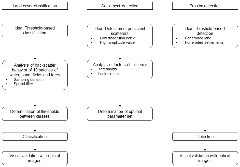
Figure 1 Overview of the analytical strategy to develop an algorithm detecting eroded farmland and settlement.

2.3 Land cover classification

To get a visual impression of the backscattering characteristics of different land cover types, the average backscatter coefficient of five classes (settlement, trees, fields, sand and water) was plotted for the period from January 2018 to February 2020. For each of the four land cover classes, water, sand, trees and agricultural fields, 10 patches of size 100×100 m were chosen based on visual inspection of the optical satellite images provided by the GEE. For each class, the 10 patches were distributed along the length of the Jamuna River. The locations of the patches are shown in Fig. A1.

The speckle inherent in SAR images can be reduced by temporal averaging (maintaining spatial resolution but requiring several images) or by spatial filtering (requiring only one image but reducing spatial resolution). There exists, thus, a tradeoff between keeping full spatial resolution and using only a few images. To assess riverbank erosion in Bangladesh, it would be ideal to use only a few images (to obtain the assessment as early as possible after the end of the monsoon season) while maintaining spatial resolution (to have a precise estimate of the erosion extent). Therefore, a compromise has to be found between sampling duration and spatial resolution. We tested the influence of these two parameters for a range of configurations:

• Eight sampling durations – 2 weeks; 1 month; and 2, 3, 4, 5, 6, and 7 months. Each of these eight periods started on 1 November 2018. All images within the respective period were averaged temporally before the subsequent analysis.

• Seven spatial filters – no filter; 3×3 refined Lee filter; and 3×3, 5×5, 7×7, 25×25 and 50×50 boxcar filter (Lee, 1981; Lee et al., 2009). The filters were applied to the absolute backscatter values.

For a certain imaging configuration (sampling duration and filter type), the mean backscatter and the standard deviation of the pixels within each patch were calculated. Subsequently, these 10 patch-specific mean and standard deviation values were averaged to yield 1 mean backscatter and 1 standard deviation value per land cover class and imaging configuration.

To classify pixels into one of the four classes, thresholds were defined between water and sand, sand and fields, and fields and trees. The thresholds were calculated as

$$\mathrm{0.5}\times \left[({\text{mean}}_i+n\times {\mathit{\sigma }}_i)+\left({\text{mean}}_j-n\times {\mathit{\sigma }}_j\right)\right],$$

where i and j indicate the class with the lower and higher mean backscatter, respectively. n was chosen as the largest natural number such that (mean${}_i+n\times {\mathit{\sigma }}_i$) and (mean${}_j-n\times {\mathit{\sigma }}_j$) would not overlap. n could thus be different for each pair of classes. For trees, an additional upper threshold was set at −2 dB to distinguish them from settlements. Pixels were classified according to their backscatter value with respect to these thresholds. For instance, a pixel with a backscatter value larger than the threshold water–sand but smaller than the threshold sand–fields was classified as “sand”. The quality of the classification was assessed visually using optical Sentinel-2 images.

2.4 Settlement detection

Since houses in rural Bangladesh are typically surrounded by trees, they are not fully visible on satellite images. Moreover, they cover only small areas compared to water, sand or farmland. Therefore, they cannot be well detected with the classification approach presented in Sect. 2.3, which involves spatial averaging.

To detect houses, we exploit the fact that unlike vegetation, houses do not move or change substantially over time. Due to this low temporal decorrelation, houses are treated as persistent scatterers (PS) (Ferretti et al., 1999). Processing PS candidates in radar images usually implies analyzing the interferometric phase, which cannot be done in GEE where only amplitude information is available. However, Ferretti et al. (2001) show that phase dispersion can be estimated from the amplitude dispersion index ${\mathit{\sigma }}_A/m_A$, where m_A and σ_A are the mean and the standard deviation of the amplitude values, respectively. PS can then be selected by computing the dispersion index of each pixel from a stack of several SAR images of the same scene and keeping only those pixels exhibiting a low dispersion index. The typical range of threshold values for the dispersion index goes from 0.25 (Ferretti et al., 2001) to 0.4 (van Leijen, 2014).

Houses are not the only structures than can have a low dispersion index. Bare surfaces, for instance, might also be relatively stable over time. Therefore, we combine the dispersion criterion with an amplitude threshold: pixels are selected as PS candidates and hence houses if they show a low dispersion index and a high absolute backscatter over a series of radar acquisitions. Two implementations of the amplitude threshold were compared: first, following Kampes and Adam (2004), a pixel is selected as the PS candidate if its normalized cross section σ₀ is above a threshold N₂ in at least N₁ images. These authors propose thresholds of −2 dB for N₂ and 0.65K for N₁, where K is the number of radar acquisitions. Second, the amplitude threshold was applied to the mean of all SAR images in the stack, instead of the individual images.

The sensitivity of the settlement detection was tested for the following parameters.

• Thresholds. For the dispersion index, threshold values of 0.25 and 0.4 were tested. For the amplitude threshold, −4, −2 and 0 dB were analyzed. These analyses were done for a sampling duration of 6 months starting 1 November 2019.

• Look direction. Since the roofs of buildings typically have a specific orientation, they are likely to have a stronger backscatter for one of the two look directions – ascending or descending. Therefore, these two types were compared.

2.5 Erosion detection

In examining the impact of riverbank erosion on human livelihoods along the Jamuna River, we are interested in two effects, which are treated separately: erosion of land (farmland or trees) and erosion of houses. Land was identified as eroded in one specific monsoon season if it was classified as “field” or “trees” before the monsoon season and as “sand” or “water” afterwards. Erosion to sand and erosion to water were not differentiated further since in both cases the land cannot be used for agriculture anymore, which is the main effect we are interested in this application.

For classifying the land, a sampling duration of 6 months (November to April) was used for all years from 2014/15 to 2018/19. For 2019/20, only the images from November 2019 were used to simulate the case where the erosion detection has to be performed already in December after the end of the monsoon. A 7×7 boxcar filter was applied to create smooth and continuous erosion bands. The threshold discriminating sand/water from fields/trees was −13.2 and −12.7 dB for the case where 6 months and 1 month of data were used, respectively (Tables B1 and B2). To detect eroded settlements, a similar strategy was followed: a pixel was selected as settlement eroded during a specific monsoon season if it was classified as “settlement” before the monsoon and as “sand” or “water” afterwards. The final algorithm to detect eroded farmland and settlement is schematized in Fig. 2.

Figure 2 Flowchart of the final implementation to detect eroded farmland and settlement. THR: threshold.

2.6 Accuracy assessment

Since our study area is large (spanning more than 200 km from north to south), it was not feasible to collect sufficient ground-truth data to validate our land cover classification algorithm. To still be able to judge its accuracy, we compared the SAR-based classification to an independently conducted classification based on optical Sentinel-2 imagery, performed in the GEE.

Classification of Sentinel-2 images was based on the normalized difference vegetation index (NDVI). The NDVI takes on values between −1 and 1. In terms of the land cover classes relevant for our study, water bodies typically exhibit NDVI values below 0, bare ground between 0 and 0.1, and cultivated land above 0.1 (DeFries and Townshend, 1994; Huang et al., 2020).

Since the detection of eroded farmland relies only on the threshold between sand and vegetation (see Sect. 2.5), we differentiated only two land cover classes in the Sentinel-2 classification: sand/water (corresponding to all pixels exhibiting an NDVI value <0.1) and vegetation/trees (corresponding to all pixels exhibiting an NDVI value >0.1). While this is a large simplification, it serves the purposes of this study where we try to detect land that changes from vegetated before the monsoon to sand or water after the monsoon.

The pixel-level accuracy of the SAR-based classification was assessed for one site by counting all pixels which were (a) identically classified as vegetation by both methods, (b) false positives (classified as vegetation by the SAR-based method and as sand/water by the Sentinel-2-based method), and (c) false negatives (classified as sand/water by the SAR-based method and as vegetation by the Sentinel-2-based method).

The quality of Sentinel-2 images depends on cloud cover. In Bangladesh, cloud cover varies seasonally, with the highest values occurring during the monsoon (June to September) and the lowest values in the dry season (November to March) (Fig. A2). Therefore, the accuracy assessment was performed for the 2 months with the lowest cloud cover (November and March), using the 1-month median NDVI value. For both November and March, the accuracy assessment was repeated for 3 consecutive years (2018/19 to 2020/21). The code for the Sentinel-2-based assessment is contained in the GEE code referenced in Sect. 2.2.

3 Results

3.1 Determination of thresholds for land cover classification

The average monthly backscatter of seven patches is shown as a time series in Fig. 3. The settlement and tree patch are the most stable since they are neither affected by (rapid) vegetation growth nor affected by monsoon flooding. The river patch has mostly the lowest coefficient, which increases during the monsoon, potentially due to wind and rain disturbing the flat water surface. While fields generally have a backscatter coefficient close to that of trees, they can be seasonally flooded during the monsoon (field 2) or completely eroded (field 3). From the behavior of field 2, the dry season can be defined as the period between November and June of the following year (indicated by the vertical lines). The sand patch lies in between water and fields.

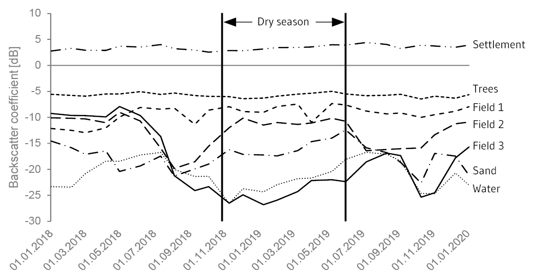
Figure 3 Mean monthly backscatter of different land cover types (one patch per type; the location of the patches is shown in Fig. A1) between January 2018 and February 2020, obtained from the C band of Sentinel-1. Per month, between one and six images are averaged.

The average backscatter of the 10 sand patches is shown in Fig. 4a as a function of different sampling durations and filter configurations. For a given filter, there is no significant variation of the backscatter value with increasing sampling duration. For a given sampling duration, the average backscatter increases slightly with increasing filter size. However, this increase becomes statistically significant at the 95 % level only for the largest filters (25×25 and 50×50 pixels). For such large filters (50×50 pixels corresponds to 500×500 m), this is probably caused by other land cover classes with a higher backscatter value (e.g., fields) being included into the filter window.

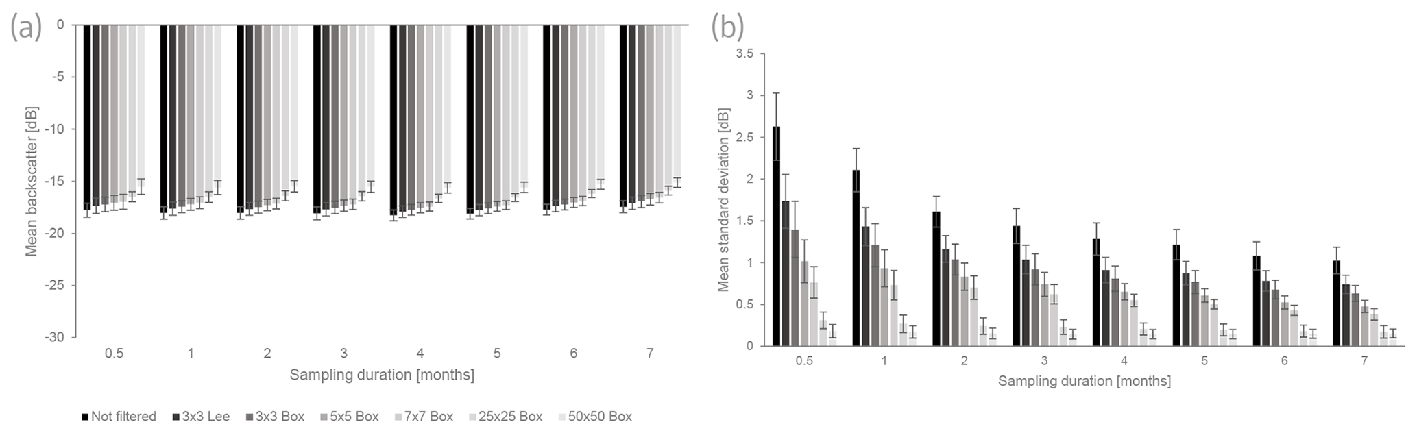
Figure 4 Average backscatter (a) and average standard deviation (b) of the pixels within 10 patches of sand for different sampling durations and filter sizes. Bars indicate the 95 % confidence interval. Lee – Lee filter. Box – boxcar filter.

Figure 4b presents the standard deviation of all pixels within one patch, averaged over the 10 sand patches. For a given filter, the standard deviation decreases with increasing sampling duration. For a given sampling duration, it decreases with increasing filter size. These observations correspond to the two mechanisms for speckle reduction outlined in Sect. 2.3, namely temporal averaging and spatial filtering. The other three land cover classes, water, fields and trees, show similar tendencies for filter size and sampling duration, both for average backscatter values and standard deviations (Fig. A3).

These findings allow defining thresholds to separate the four classes in the land cover classification. As discussed in Sect. 2.3, each combination of sampling duration and filter size has a certain advantage and a certain disadvantage. To illustrate this tradeoff, two extreme combinations are compared in Fig. A4. In practice, a compromise between these two extremes seems more likely, meaning that some spatial resolution has to be given up when a slightly longer sampling duration is used. One example for such a compromise is presented in Fig. 5, for which images from 1 month have been filtered with a 3×3 boxcar filter.

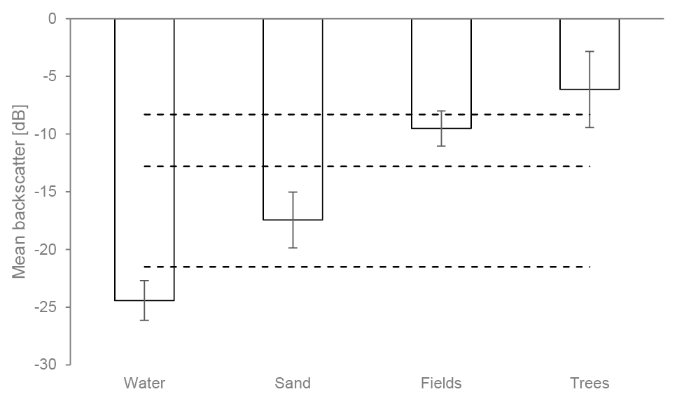
Figure 5 Average backscatter for four land cover classes for a sampling duration of 1 month and a 3×3 boxcar filter. Bars indicate the mean ±2 standard deviations. Horizontal lines indicate the thresholds between the respective classes.

The determination of the thresholds is illustrated in Table 1 for the case of 1-month sampling duration and a 3×3 boxcar filter. As can be seen in Fig. 5, the bars of fields and trees overlap if 2 standard deviations are used. However, they do not overlap if only 1 standard deviation is used. Hence, intervals with 1 standard deviation are used to determine the threshold between fields and trees. For water–sand and sand–fields, the intervals do not overlap even if 3 standard deviations are considered. Therefore, 3 standard deviations are used to calculate the respective thresholds. The thresholds for the two configurations from Fig. A4 are contained in Tables B3 and B4. The average backscatter values shown in Tables 1, B3 and B4 compare reasonably well to reference values from the literature (Table B5).

Table 1 Determination of thresholds for a sampling duration of 1 month and a 3×3 boxcar filter. Values in bold are those that have been used to calculate the threshold indicated in the last column. All values are in decibels (dB). μ – mean. σ – standard deviation.

Assuming the backscatter values in each class to be distributed normally around the mean, this approach allows an estimation of the accuracy of the resulting classification. In a normal distribution, 68 %, 95 % and 99.7 % of all values lie within mean ±1, 2 and 3 standard deviations, respectively. As the thresholds water–sand and sand–fields are based on the interval with 3 standard deviations, we thus expect less than 0.15 % of all water pixels to be incorrectly classified as sand pixels. The same percentage applies for sand pixels being incorrectly classified as water/field pixels and for field pixels being misclassified as sand pixels. For fields–trees, only 1 standard deviation has been used, and hence 16 % of all field and tree pixels are expected to be falsely classified as tree and field pixels, respectively.

Trees and fields can thus not be well distinguished in this setup. This shortcoming is, however, negligible in the context of studying riverbank erosion. Here, the focus is on land covered by fields or trees being eroded and appearing as sand or water afterwards. Therefore, the most important threshold is the one between sand and fields, which yields higher accuracy.

The classification resulting from these three imaging configurations is depicted in Fig. 6 with an optical Sentinel-2 image as the baseline. If only 2 weeks are sampled with a 25×25 boxcar filter, the spatial resolution is largely lost (panel b). If, by contrast, no filter is applied and 6 months are sampled, the classification remains very fine grained (panel c). However, the distinction between sand and water is not very accurate. The compromise – 1-month sampling duration and a 3×3 boxcar filter (panel d) – manages to preserve a large degree of spatial resolution while distinguishing well between the four classes. It thus seems the most appropriate of these three imaging configurations.

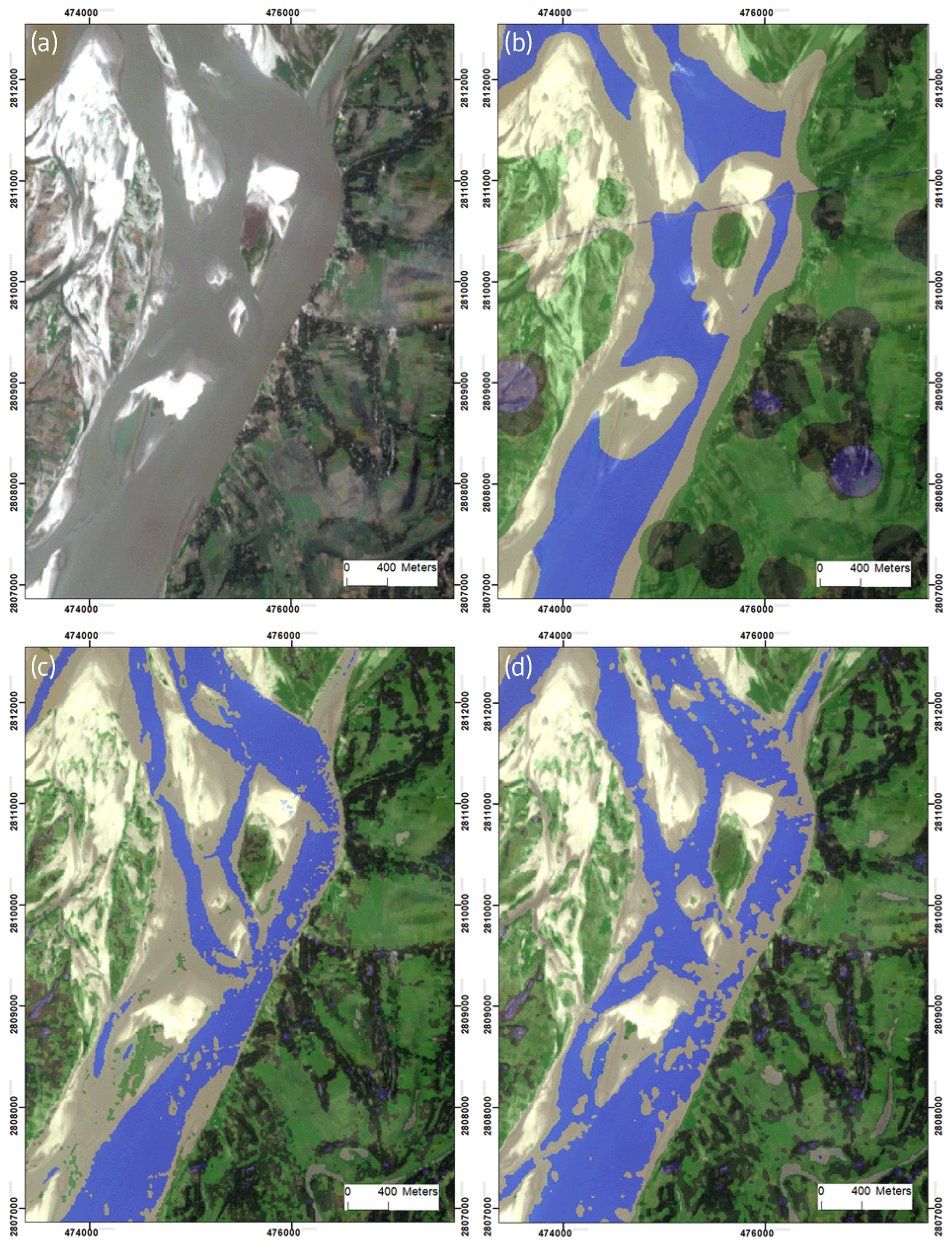
Figure 6 (a) Sentinel-2 image of a stretch of the eastern riverbank of Jamuna River, taken in November 2019. Image dimensions: ca. 4.5×6 km. (b, c, d) Classification result for a sampling duration of 2 weeks and a 25×25 boxcar filter, 6 months and no filter, and 1 month and a 3×3 boxcar filter, respectively. Blue – water; sand – sand; light green – fields; dark green – trees. Source of optical background image: Sentinel-2. The location of the patch is shown in Fig. A1 (patch 1). Coordinates in this and all other maps are in Gulshan 303 Bangladesh TM (EPSG 3106).

3.2 Detection of settlement as persistent scatterers

Figure A5a illustrates the need to apply an amplitude threshold in addition to the dispersion index. If only the dispersion index is used to classify settlements, many vegetation pixels that happen to be stable over the sampled time window are misclassified as settlements. The influence of the dispersion index threshold and the amplitude threshold is shown in Fig. 7. For the dispersion index, a threshold of 0.25 (panel b) selects only very stable pixels as PS candidates. Accordingly, fewer pixels are selected than for a threshold of 0.4 (panel a). For the amplitude threshold, the effect is the opposite: applying a threshold of −4 dB (red) selects more pixels as PS candidates than for −2 dB (blue) or 0 dB (orange). While the threshold of −4 dB thus seems to select more settlement pixels (e.g., upper-left corner of panel a), also the risk of misclassifying tree pixels as settlements rises.

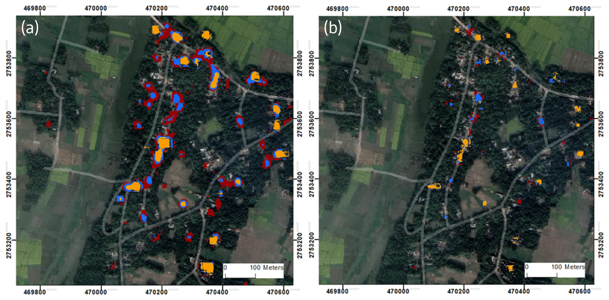
Figure 7 Influence of classification thresholds on settlement detection. Shown are dispersion index thresholds of 0.4 (a) and 0.25 (b) – the lower the threshold, the more stable a pixel has to be for it to be classified as a PS candidate. Colors correspond to different values of the amplitude threshold: −4 dB (red), −2 dB (blue) and 0 dB (orange) – the lower the threshold, the higher the chance of classifying tree pixels as settlement pixels. Source of optical background image: Google, © 2020 Maxar Technologies, CNES/Airbus.

For our application, however, we are rather interested in detecting the rough location of settlements than in precisely distinguishing settlement and 3 pixels. In fact, trees are often planted around houses, making them good indicators of settlements. As too few settlement pixels are detected in panel (b), we suggest a threshold combination of 0.4 and −4 dB for the dispersion index and the amplitude, respectively. Still, it is important to note that, even with this combination (red pixels in panel a), several pixels that appear as houses in the optical image are not detected. We should thus keep in mind that what the algorithm classifies as settlement is most likely indeed a settlement but that it cannot detect all settlements, especially if they are covered by trees.

The influence of the look direction is illustrated in Fig. A5b. The overlap between the ascending and descending orbit is small. This corresponds to the fact that each building has a specific orientation of its roof. Therefore, some roofs have a stronger backscatter in the descending orbit, while others reflect more in the ascending orbit. Similar effects can be expected if persistent scatterers are located on walls or in corners of buildings. For maximum settlement detection, it is thus recommended to use SAR images of both look directions. To conclude, the recommended set of parameters to detect settlements is to use an amplitude and dispersion index threshold of −4 dB and 0.4, respectively, using images of both ascending and descending orbit.

3.3 Detection of eroded farmland and settlements

Figure 8 illustrates the result of the erosion detection (both farmland and settlements) for one specific site for the monsoon seasons 2018 and 2019. To evaluate the quality of the erosion detection, the detected erosion patches are mapped on optical images from before and after the monsoon. The results of the overall validation of the land cover classification are contained in Sect. 3.4.

The focus of the project is on erosion occurring on the outer riverbanks of the Jamuna. Therefore, erosion happening on the sandbanks and islands in the river is omitted in the following discussion, which focuses exclusively on the long strip of eroded land on the outer riverbank. For both years, all that has been detected as eroded land has entirely been land before the monsoon (left column) and completely water after the monsoon (right column). For these examples, there is thus no type-I error, i.e., classifying land as eroded when it is not.

There is, however, a type-II error, i.e., eroded land that is not classified as such. This error tends to be small and thus negligible for the overall purpose of detecting sites where erosion occurred to a significant extent. Lastly, the algorithm can distinguish well between eroded farmland and eroded sand, as can be seen in the lower-left corner of the 2019 image before the monsoon. Regarding the patches detected as eroded settlements (bright red), by far not all of the eroded settlement is detected. Again, this type-II error is negligible given the purpose of detecting those sites that have seen erosion of settlement in general. For this, it is not necessary to detect every single house that has been eroded.

The erosion detection works for the monsoon seasons from 2015 to 2019, since Sentinel-1 images are only available from October 2014 onwards. Figure 9a shows the sequential nature of erosion, which does not occur at random locations, but typically in sites which have already experienced erosion during the previous monsoon season(s). We can also see the highly dynamic nature of land accretion and erosion. For instance, an island had formed at the place where land had been before the 2015 monsoon. Part of this island has been eroded again in the 2019 monsoon season (orange patch overlaying the dark brown 2015 erosion band). Further, settlements have been eroded in all five monsoon seasons (blue dots). Figure 9b shows where land was eroded in the 2019 monsoon along a larger section of the Jamuna River. Erosion occurred within but to a large extent also outside of the hotspot areas predicted by CEGIS (2018).

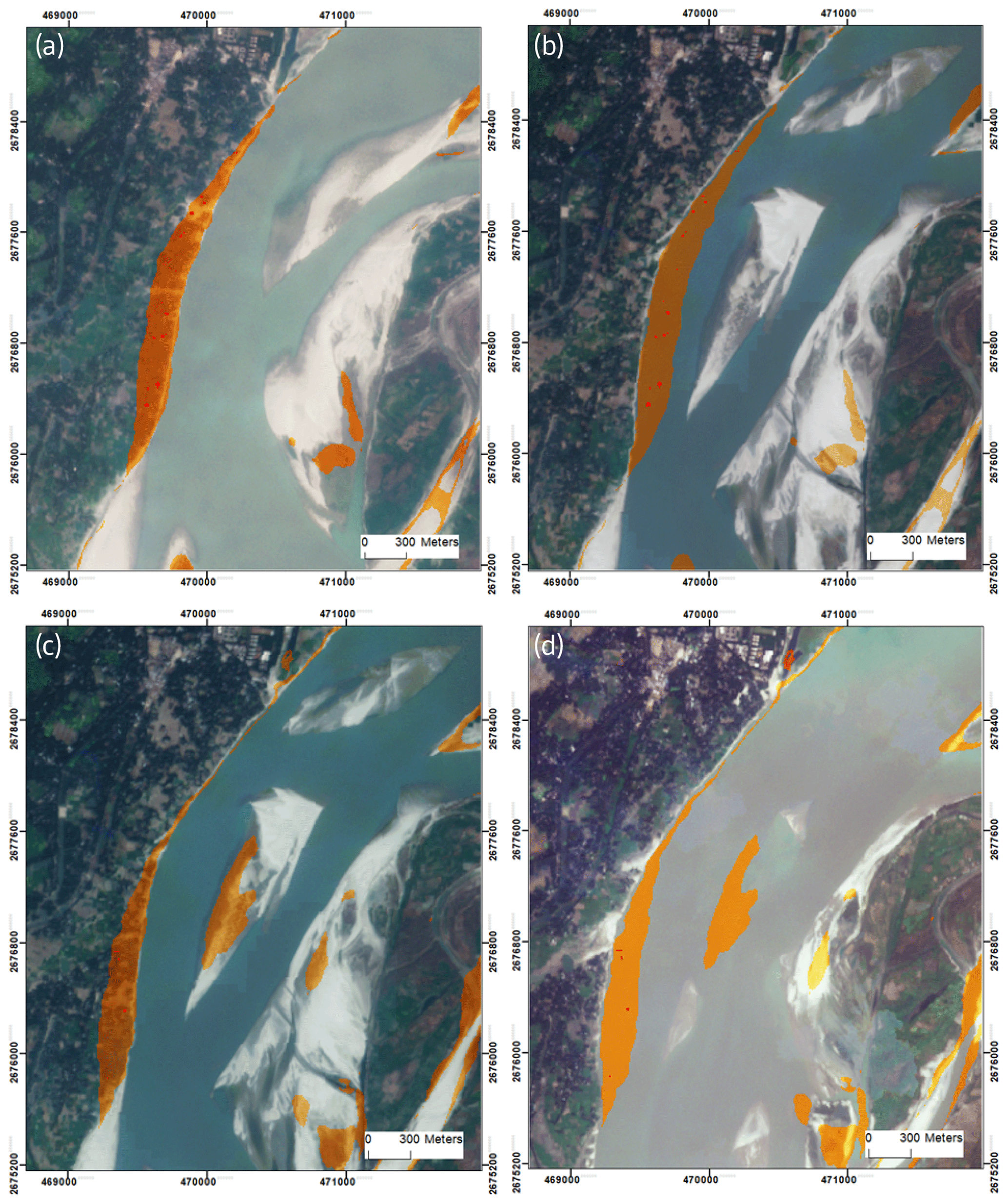
Figure 8 Validation of erosion detection. Shown are eroded land (orange) and eroded settlements (red) for 2018 (a, b) and 2019 (c, d). Baseline: optical Sentinel-2 images from before (a, c) and after (b, d) the monsoon. The location of the patch is shown in Fig. A1 (patch 3).

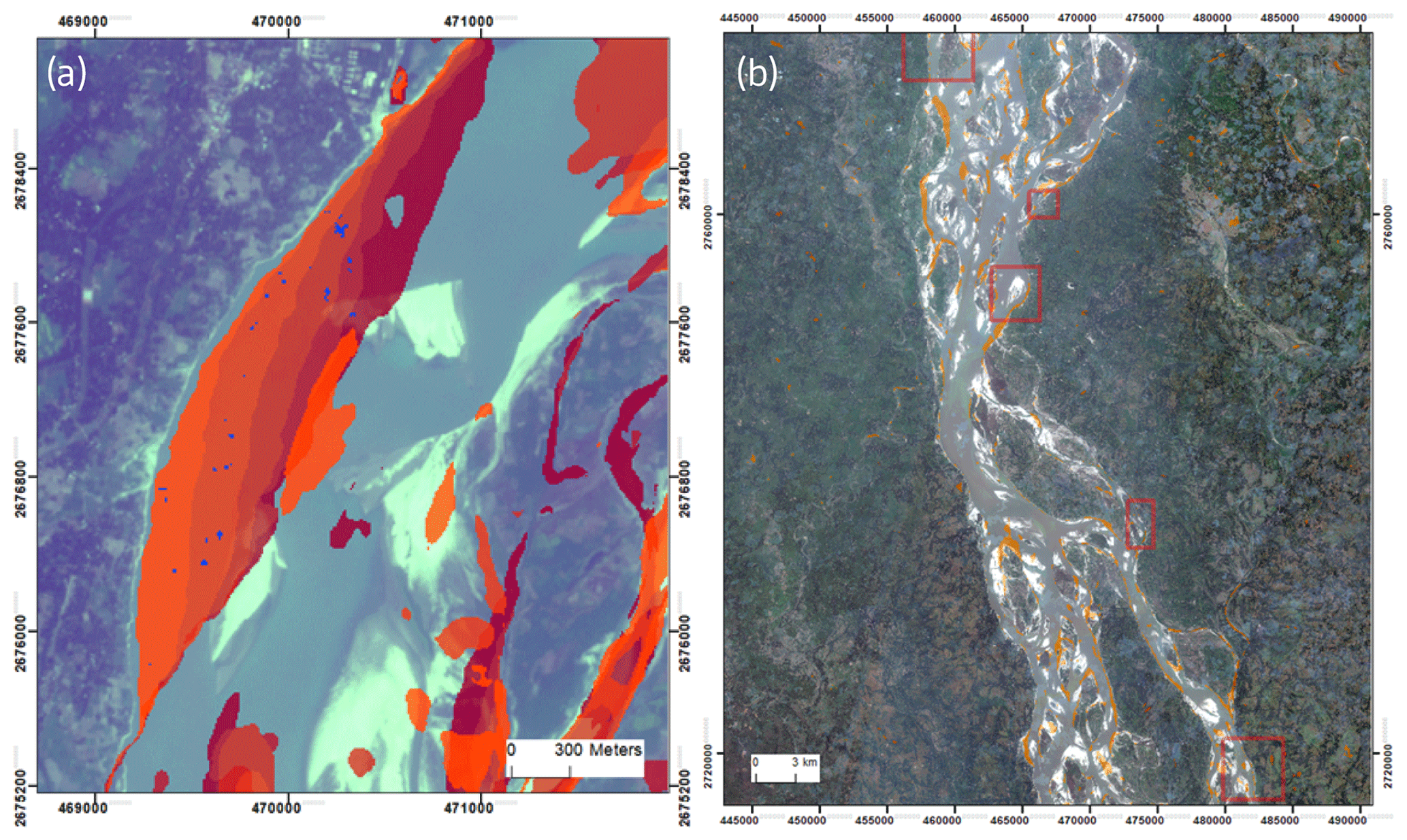
Figure 9 (a) Detected erosion for the monsoon seasons 2015 (dark red) to 2019 (light red). Blue: eroded settlements. (b) Locations of land eroded during the 2019 monsoon (orange). The red rectangles are the locations for which CEGIS (2018) predicted severe erosion. Source of optical background images: Sentinel-2.

3.4 Accuracy assessment

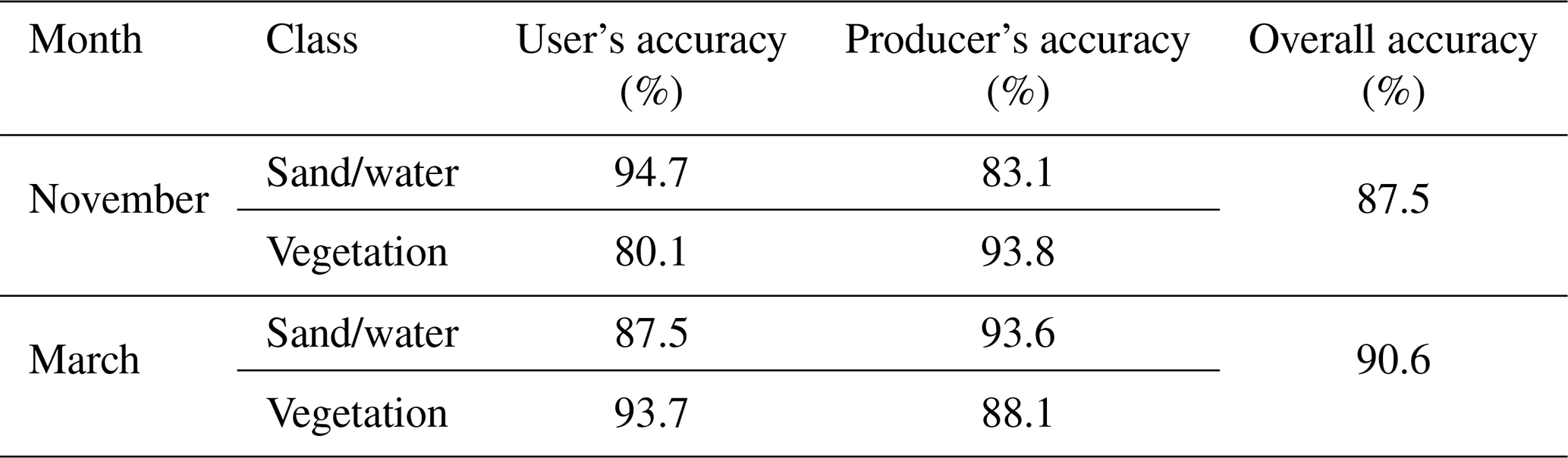
A confusion matrix of vegetation versus sand/water was calculated for 6 different months (Table B6). The accuracy metrics were averaged over 3 consecutive years for both November and March (Table 2). The classification showed a satisfactory accuracy over 87 %. The observed errors might be introduced by the cloud mask which is applied to the Sentinel-2 images and potentially leads to misclassified pixels.

Table 2 Accuracy assessment of the SAR-based classification for 2 months. Indicated are the accuracy values averaged for November/March over 3 consecutive years.

As mentioned in Sect. 2.6, a validation based on ground-truth data was not possible due to the large size of our study area. Readers and users are, however, invited to access the source code in the GEE and compare the SAR-based land cover classification to optical imagery for specific sites of interest.

3.5 Final implementation

Finally, the results from Sect. 3.1 to 3.3 were implemented in a GEE-based analysis tool that allows the user to explore where erosion of farmland and settlement has occurred during the five monsoon seasons from 2015 to 2019. The tool contains the following information:

• five layers for land eroded in the five monsoon seasons, 2015 to 2019;

• five layers for settlements eroded in the five monsoon seasons, 2015 to 2019;

• one layer for the settlement detected in the beginning of 2020;

• three optical images from January 2018, 2019 and 2020 as a visual baseline;

• the 14 “erosion hotspots” identified by CEGIS in their 2019 erosion prediction (cf. Sect. 1).

The GEE-based tool to assess riverbank erosion using Sentinel-1 data and a short video tutorial to introduce users who are unfamiliar with the GEE to the application of this tool are referenced in the section “Code availability”.

4 Discussion

Various studies have investigated riverbank erosion along the Jamuna applying remote sensing approaches (Hassan et al., 2017; Khan et al., 2022; Pahlowan and Hossain, 2015; Islam, 2009). All of them, however, used optical images, which are available only at cloud-free daylight conditions. Our study is the first to assess riverbank erosion along the Jamuna using radar satellite images, which are independent of daylight or weather conditions. Hence, they are more readily available after the end of the monsoon season and thus better suited to inform practitioners who are supporting local communities to prepare for the upcoming monsoon and erosion season. In terms of accuracy, our algorithm performed satisfactorily when compared to an approach based on optical images (see Sect. 3.4).

Still, different limitations might affect the results of this study. First, as outlined in Sect. 2.1, the GEE contains only the amplitude but not the phase values of radar images. The phase value contains information on the distance between the sensor and the ground, accurate to a small fraction of the radar wavelength. One powerful technique employing the phase value is SAR interferometry, which compares for one scene the phase of two or more radar images acquired from different positions or at different times (Moreira et al., 2013). Accessing the phase information could thus open up alternative strategies to detect eroded land, for instance from temporal decorrelation. SAR interferometry, however, requires special software, which might not be available in resource-constrained settings. The GEE, by contrast, is easy and free to use, making the developed algorithm accessible to authorities and researchers in Bangladesh.

Second, our study used only radar data. Combining optical and SAR data generally yields an improved performance compared to using any of the two alone. Examples using both data types include land cover classification (Carrasco et al., 2019; Miettinen et al., 2019; Poortinga et al., 2019; Zhang et al., 2018), change detection (Canty and Nielsen, 2017; Celik, 2018; Shimizu et al., 2019) and the derivation of river discharge for the upper Brahmaputra River (Huang et al., 2018). The GEE facilitates the combination of optical and SAR data. Such a combination would thus be another strategy to further improve the results of this study.

Third, we have developed the algorithm to detect riverbank erosion for one specific case study. As it is usually the case for case study research, it is not evident how well our findings can be transferred to other contexts beyond Bangladesh. Given, however, that the basic mechanism of riverbank erosion (vegetated/settlement land turning into sand/water) is identical irrespective of where erosion occurs, we believe that it is possible to apply our erosion detection approach to other contexts at relatively low effort (e.g., by adapting classification thresholds to local vegetation/soil types). We invite interested readers – both from research and from practice – to access our algorithm and to apply it to other geographical settings.

5 Conclusions

We have implemented and applied a GEE-based method to quantitatively assess riverbank erosion along the Jamuna River in Bangladesh based on Sentinel-1 GRD intensity data. Timely detection of riverbank erosion is an essential element of disaster risk management yet especially challenging in resource-limited settings.

We investigated whether the locations of past erosion events can be extracted from Sentinel-1 SAR imagery. We developed an algorithm to classify land cover, identify settlements, and detect eroded farmland and settlements along the Jamuna River. The SAR-based classification approach can provide information on where land and settlements have been eroded during the last monsoon already 1 month after the end of the monsoon season and hence potentially earlier or at least more reliably than using optical satellite images, which depend on cloud-free conditions. This erosion detection can be achieved at sufficiently high spatial resolution. We could thus demonstrate the suitability of radar imagery to assess past erosion events.

The analysis was performed using the GEE, which gives access to Google's cloud computing infrastructure as well as to massive amounts of satellite imagery, including time series of Sentinel-1 GRD backscatter data and Sentinel-2 optical data on a global scale. A limitation of using the GEE is that it contains only the amplitude values and not the phase values of the radar images. Land cover change classification approaches using interferometric coherence can thus not be implemented in the GEE. However, the GEE facilitates sharing and re-using algorithms, making the results of this study accessible and useable for government agencies or non-governmental organizations (NGOs) in Bangladesh. To share our results, we developed an interactive online tool allowing the user to explore where farmland and settlement have eroded along the Jamuna River in the monsoon seasons 2015 to 2019. This online tool as well as the underlying source code can be accessed and adapted free of charge, making it an attractive tool to use in resource-constrained settings.

Spatiotemporally consistent sequences of progressive riverbank erosion give valuable insights on where erosion will likely occur in the following monsoon season. Such information can be used to alert potentially affected residents accordingly. Likewise, the results of our study can be used to inform researchers or NGOs working on the adaptation of the population living along the Jamuna to the riverbank erosion. As such, the tool developed in this study might be of interest to both policymakers and practitioners working in the fields of disaster risk management and communication. Since riverbank erosion is a phenomenon occurring along many of the world's major rivers (e.g., Mekong River, Yellow River, Mississippi River or Danube River), the relevance of our tool extends beyond the specific case study of Bangladesh. Likewise, it might be applicable to coastal erosion – another environmental hazard that is bound to increase in the age of climate change.

Appendix A: Additional figures

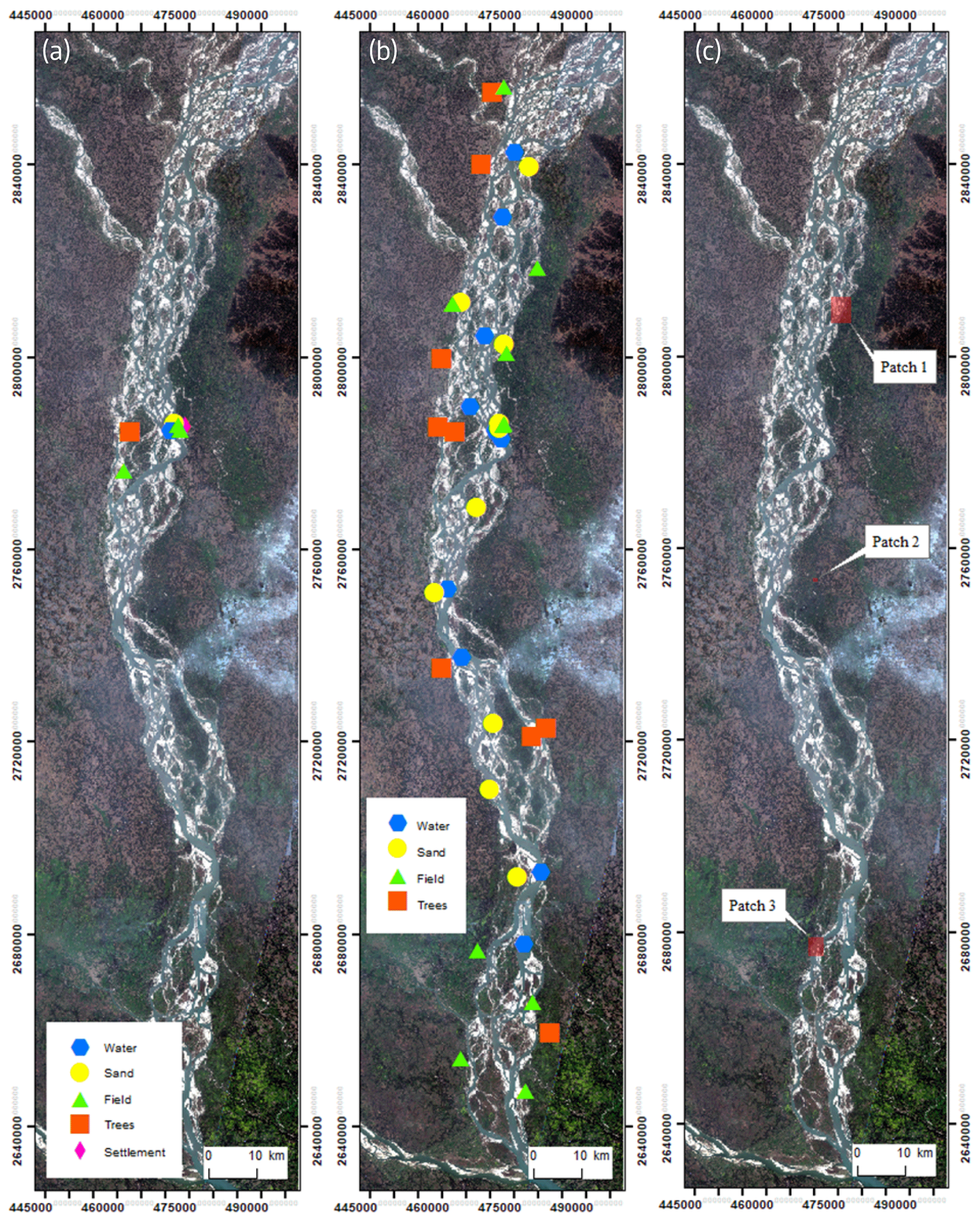
Figure A1 (a) Locations of the patches shown in Fig. 3 (symbols are larger than the patches). (b) Locations of the patches analyzed for the development of the land cover classification (symbols are larger than the patches). (c) Locations of the patches used to validate the land cover classification (patch 1), the settlement detection (patch 2) and the erosion detection (patch 3). Exact coordinates for all patches are contained in the GEE source code. Source of optical background image: Sentinel-2.

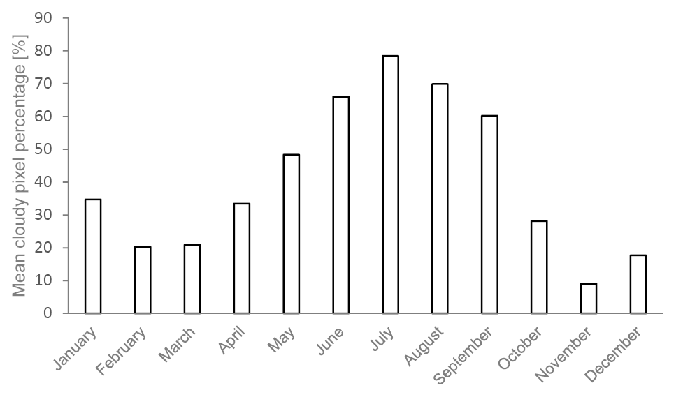
Figure A2 Mean cloudy pixel percentage of all Sentinel-2 images taken over the assessment site during the respective month. For each month, 5 consecutive years were analyzed. The plotted values represent the average of these 5 years.

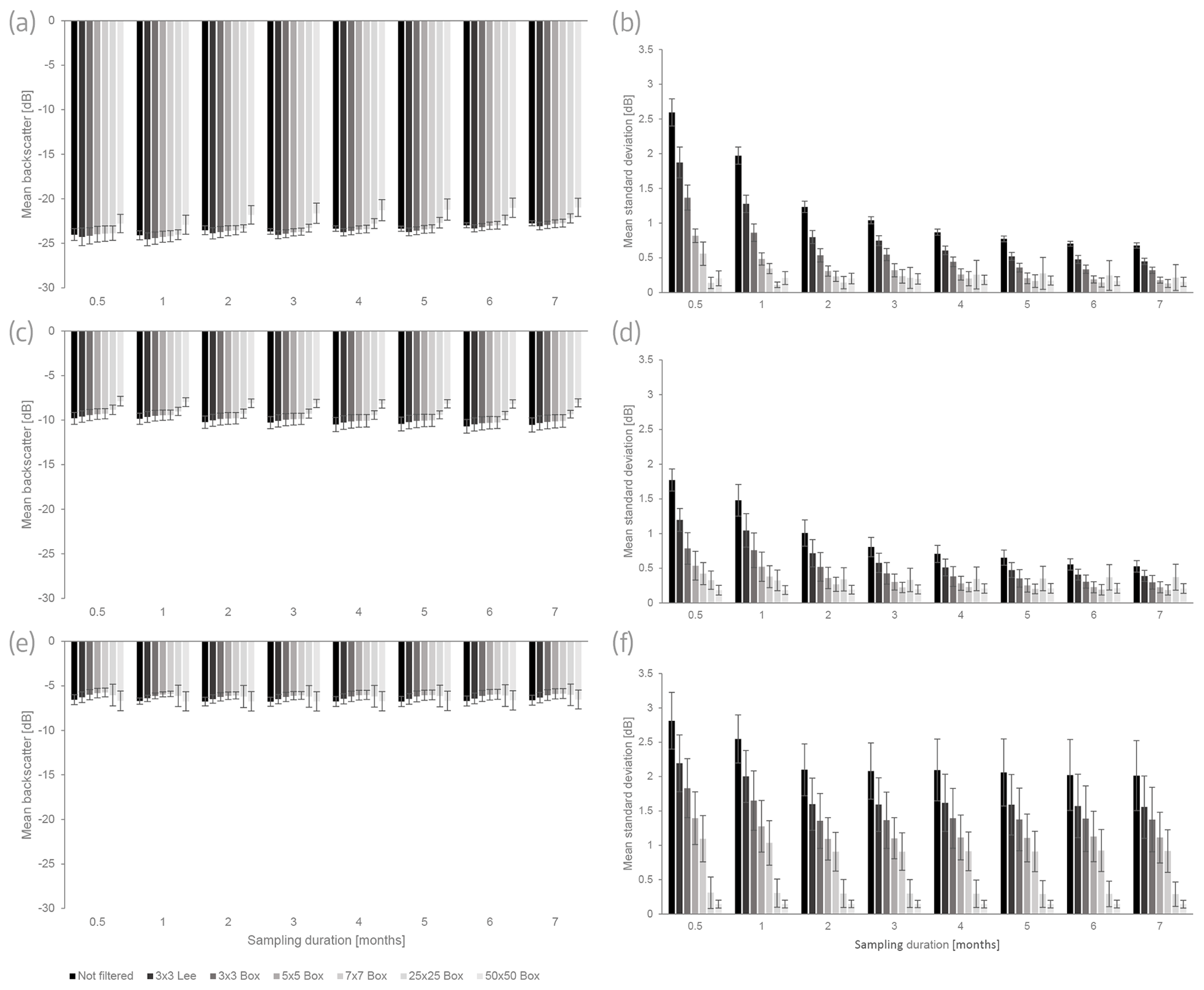
Figure A3 Average backscatter (a, c, e) and average standard deviation (b, d, f) of the pixels within 10 patches of water (a, b), fields (c, d) and trees (e, f) for different sampling durations and filter sizes. Bars indicate the 95 % confidence interval. Lee – Lee filter. Box – boxcar filter.

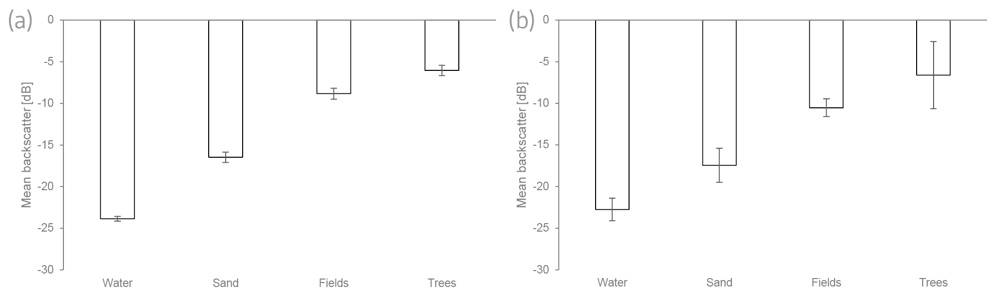
Figure A4 Average backscatter for four land cover classes (a) for a sampling duration of 0.5 months and a 25×25 boxcar filter and (b) for a sampling duration of 7 months and no filter. Bars indicate the mean ±2 standard deviations. If images are available only from 2 weeks, strong spatial filtering (25×25 pixels) reduces the standard deviation enough to separate all four classes even at the level of 2 standard deviations around the mean (a). If, by contrast, images are available from 7 months, water, sand and fields can be separated even if no spatial filter is applied (b). In this setting, fields and trees can be distinguished only at the level of 1 standard deviation around the mean (not shown in the graph).

Figure A5 (a) Classification of settlements using the dispersion index only (blue) or the combination of dispersion index and amplitude threshold (orange). Thresholds: 0.25 (dispersion index); −2 dB (amplitude). (b) Settlement detection for ascending (orange) and descending (blue) orbit. Thresholds: 0.4 (dispersion index); −4 dB (amplitude). Sampling duration for both panels: 6 months. The location of the patch is shown in Fig. A1 (patch 2). Source of optical background image: Google, © 2020 Maxar Technologies, CNES/Airbus.

Appendix B: Additional tables

Table B1 Determination of thresholds for a sampling duration of 6 months and a 7×7 boxcar filter. Values in bold are those that have been used to calculate the threshold indicated in the last column. All values are in decibels (dB). μ – mean. σ – standard deviation.

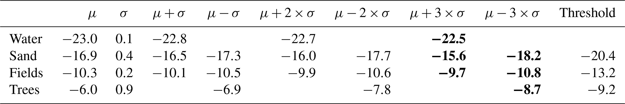
Table B2 Determination of thresholds for a sampling duration of 1 month and a 7×7 boxcar filter. Values in bold are those that have been used to calculate the threshold indicated in the last column. All values are in decibels (dB). μ – mean. σ – standard deviation.

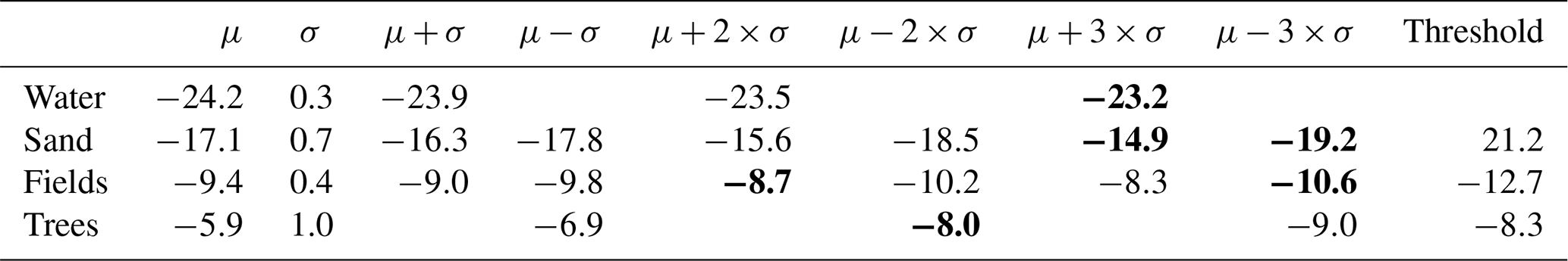
Table B3 Determination of thresholds for a sampling duration of 2 weeks and a 25×25 boxcar filter. Values in bold are those that have been used to calculate the threshold indicated in the last column. All values are in decibels (dB). μ – mean. σ – standard deviation.

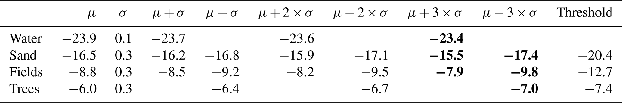
Table B4 Determination of thresholds for a sampling duration of 7 months, unfiltered. Values in bold are those that have been used to calculate the threshold indicated in the last column. All values are in decibels (dB). μ – mean. σ – standard deviation.

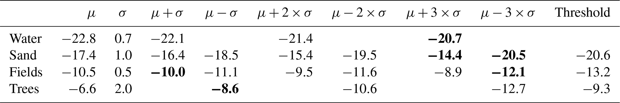
Table B5 Average backscatter values from Ulaby and Dobson (1989) for the C band at VV polarization for look angles of 30 and 45^∘.

Table B6 Confusion matrix of resultant land cover classification as obtained from SAR versus Sentinel-2 (S2) for 6 different months.