the Creative Commons Attribution 4.0 License.
the Creative Commons Attribution 4.0 License.
 | 01 Dec 2023
Machine-learning-based nowcasting of the Vögelsberg deep-seated landslide: why predicting slow deformation is not so easy
Adriaan L. van Natijne
Thom A. Bogaard
Thomas Zieher
Jan Pfeiffer
Roderik C. Lindenbergh
Landslides are one of the major weather-related geohazards. To assess their potential impact and design mitigation solutions, a detailed understanding of the slope processes is required. Landslide modelling is typically based on data-rich geomechanical models. Recently, machine learning has shown promising results in modelling a variety of processes. Furthermore, slope conditions are now also monitored from space, in wide-area repeat surveys from satellites. In the present study we tested if use of machine learning, combined with readily available remote sensing data, allows us to build a deformation nowcasting model. A successful landslide deformation nowcast, based on remote sensing data and machine learning, would demonstrate effective understanding of the slope processes, even in the absence of physical modelling. We tested our methodology on the Vögelsberg, a deep-seated landslide near Innsbruck, Austria. Our results show that the formulation of such a machine learning system is not as straightforward as often hoped for. The primary issue is the freedom of the model compared to the number of acceleration events in the time series available for training, as well as inherent limitations of the standard quality metrics such as the mean squared error. Satellite remote sensing has the potential to provide longer time series, over wide areas. However, although longer time series of deformation and slope conditions are clearly beneficial for machine-learning-based analyses, the present study shows the importance of the training data quality but also that this technique is mostly applicable to the well-monitored, more dynamic deforming landslides.
- Article
(7640 KB) - Full-text XML
- BibTeX
- EndNote


Landslides make up 6 % of the weather-related disasters globally (World Meteorological Organization (WMO), 2021). To protect the public, landslides have been a major research topic for the past decades. For local landslide mitigation by geotechnical intervention, an up-to-date understanding of these hydro-meteorological phenomena, their feedbacks, and their impact is desired. This understanding may then be leveraged for the design of landslide hazard mitigation measures.
Where the installation of effective remediation concepts is not possible, early warning systems may help to reduce the landslide risk. Such systems should quickly adapt to changing conditions, both on the slope and globally (e.g. climate change). Moreover, such a system should be fast to adapt and implement to assess as many slopes as possible.
Existing local systems typically provide early warning based on in situ slope monitoring (Guzzetti et al., 2020). An example of a satellite-based global early warning system is the LHASA model (Kirschbaum and Stanley, 2018; Hartke et al., 2020; Stanley et al., 2021) that provides a global nowcast of acute landslide susceptibility. However, these systems typically focus on sudden, fast, and shallow landslides. The literature reports mixed success in the replacement of local measurements by satellite observations for the prediction of shallow landslide collapse (Thomas et al., 2019; Yatheendradas et al., 2019). Such catastrophic events change the landscape, and as a consequence the situations before and after the collapse are no longer comparable. Therefore, the landslide process preceding the collapse can only be studied if data from before the landslide are available.
We focus on slow-moving, reactivating, deep-seated landslides on natural slopes, for which the deformation pattern is controlled by hydro-meteorological forcing. These deep-seated landslides are estimated to comprise 50 % of the landslides globally (Herrera et al., 2018; Novellino et al., 2021). The deep-seated landslides we focus on rarely evolve into catastrophic collapse and often entail a complex response to hydro-meteorological conditions controlling the landslide's pore pressure (Bogaard and Greco, 2015). They are characterized by gradual, non-catastrophic deformations that can be responsible for extensive infrastructure damage (Mansour et al., 2011). Deformation rates typically vary from millimetres to decimetres per year, whereas phases of acceleration or deceleration often correlate with time-delayed hydrological conditions (Intrieri et al., 2018).
Monitoring systems only supported by the detection of currently emerging acceleration events (e.g. Carlà et al., 2017) can only be used to detect already ongoing acceleration. As a consequence, adequate early warning is only possible if the deformation can accurately be predicted beforehand. Therefore, the deformation should be predicted from the predisposing conditions on the slope, combined with dynamic factors such as infiltrating precipitation and snowmelt that lead to higher pore pressures, instability, and subsequent deformation. However, the deformation behaviour of such slow, deep-seated landslides is “extremely difficult” to model (van Asch et al., 2007).
Past landslide deformation events are indicative of the future behaviour, as landslides are likely to display similar behaviour in similar situations (Fell et al., 2008; Guzzetti et al., 1999). Unlike catastrophic landslides, where the landslide dynamics change permanently, slow-moving landslides are not single, catastrophic incidents. Therefore, analysis of the monitoring data of deep-seated landslides is expected to reveal causal factors in landslide deformation, which allow for a continuous cycle of forecast and validation of the relationship between deformation and the conditions on the slope.
Deformation nowcasting could be considered an intermediate option between monitoring and modelling, integrating sensor data to estimate the current situation (the system state) and extrapolate on a short timescale. New data and data integration methods, “machine learning”, offer new possibilities for such data-driven landslide forecasting (van Natijne et al., 2020). Furthermore, these techniques offer new capabilities to continuously track the system state without extensive, in situ sensor networks and physics-based modelling. Such data-driven models could be used to “learn” the landslide dynamics and the interplay of hydro-meteorological factors from the deformation signal of the landslide.
In the past decades satellite observations have increased in quantity, shortening the time between subsequent acquisitions, as well as increasing the variables observed (Belward and Skøien, 2015). These acquisitions provide us with a global overview of the status of the earth at local scale, often with weekly to daily updates. More recently there is the tendency to make the data freely available, a development that lowered the barrier for innovation (Zhu et al., 2019) and especially benefits experiments that require long time series, like this study. Even though their coverage is often limited to the surface, and the spatial resolution (often kilometre range) lacks the details of close-range measurements, the repeated monitoring of the slope conditions may still reveal the slope processes responsible for accelerated deformation (van Natijne et al., 2020).
Here, we present a data-driven nowcasting model with a 4 d lead time of the deformation of the Vögelsberg landslide, near Innsbruck, Austria. We use readily available, remotely sensed data and products and test various similar remote sensing products to assess their relative performance in the nowcasting model. We discuss the complications encountered during modelling: over-parametrization, the impact of optimization metrics, and the challenges due to the deep-seated landslide inertia compared to the highly dynamic forcing of the slope.
First, we introduce the modelling options and study area. Second, we present the resources available to us, and our modelling approach, followed by the results and an extensive discussion on the insights gained during the modelling exercise. Last, we provide recommendations for future data-driven landslide nowcasting exercises.
In the present study we interpret data-driven modelling as a form of naive modelling. That is, the model is unaware of the physics behind the landslide process. For data-driven models, the deformation of the slope is merely a signal to be reproduced from a collection of observations by empirical relations, in contrast to traditional, landslide geomechanical modelling that is rooted in physics. Table C1 features a selection of studies into data-driven deep-seated landslide nowcasting, demonstrating the recent interest in this topic. Various examples come from landslides around the Three Gorges Dam that are strongly controlled by the reservoir water level (e.g. Yang et al., 2019). However, this is not the most common type of deep-seated landslide. Deep-seated landslide deformation is typically driven by water storage in the deeper subsurface. This storage is controlled by a long-term water balance of precipitation and snowmelt input, evaporation losses, and regional groundwater exchange (Bogaard and Greco, 2015). Other approaches split the deformation into a trend and predict the smaller trend deviations using a complex machine learning approach (e.g. Miao et al., 2022), although in our view the trend is an integral part of the deformation signal to be predicted.
The indirect transfer from precipitation and snowmelt to storage may be captured by, for example, including recent observations in a bucket model (Nie et al., 2017). A bucket model represents the subsoil as a storage that is replenished by precipitation and emptied by drainage and evaporation. Furthermore, changes to the storage may involve a time delay, depending on complex infiltration processes. This process may be dependent on the precipitation type, duration, and intensity. Moreover, deformation may not be governed by a short and single precipitation event. For example, a short, extreme precipitation event or 3 d of consecutive drizzle may introduce similar amounts of water to the system but will be represented differently in storage changes due to different infiltration abilities of the soil. All in all, modelling of deep-seated landslides will likely require some form of storage modelling, where these dynamics are either resolved by the model or in advance by an expert.
Two distinct modelling approaches can be distinguished. Modelling either is based on classification of the environmental conditions and associated deformation response or calculates the expected deformation response from the conditions on the slope. In either case, the model parameters are tuned on historic observations such that they best reproduce the deformation signal from the conditions observed previously at the slope. Our model of the Vögelsberg landslide is a continuous model. For completeness classification models will be introduced briefly.
2.1 Classification models
Based on the assumption that similar conditions trigger a comparable deformation response (Fell et al., 2008; Guzzetti et al., 1999), conditions and responses may be categorized. The current slope conditions are then matched against historic conditions, and the deformation response is assumed to be the same. Extrapolation of the response to previously unencountered conditions is typically impossible with these models. However, the system will therefore also not yield unrealistic results and could be considered bound to the previously encountered deformation signal.
2.2 Continuous models
The simplest, linear, model is the weighted sum of the quantified conditions at the slope. However, the slope response may not be linear and is typically not immediate. Neural networks may be used to estimate any signal by the formation of a network of interlinked nodes that ingest and combine the conditions on the slope in subsequent layers of nodes (Hornik et al., 1989; Hill et al., 1994). A time series passed to a single input neuron is equal to a weighted sum of the time series plus a bias.
As more hidden layers of neurons are introduced to the system, the direct link to the (time series) input is lost as combinations are made. Furthermore, an activation function may be applied to scale the output of each node, especially to normalize the response and filter outliers, at the cost of introducing non-linearity to the system. The number of parameters, degrees of freedom of the model, is associated with the number of input variables. When historic observations are supplied as additional observations, they will each require their own model parameters and increase the degrees of freedom in the model.
State aware models, such as recurrent neural networks (Connor et al., 1994), maintain a track record of the state of the landslide instead and iterate over the input time series in successive model runs. Individual observations are fed into the system, with the system maintaining track of their contribution to the current state of the landslide. These models resemble a bucket model, a simplified representation of the water storage in the subsoil. However, unlike in a traditional (soil moisture/ground water) bucket model, all variables are taken into account, even if they do not directly represent water. Furthermore, unlike regular neural networks, the number of trainable parameters is not dependent on the length of the history supplied to the model but on the number of memory cells and time series.
Models based on recurrent neural networks suffer from computational difficulties during optimization, where gradients may vanish (Bengio et al., 1994; Hochreiter and Schmidhuber, 1997; Hochreiter, 1998). Therefore, they are typically replaced by models based on long short-term memory (LSTM) nodes (Hochreiter and Schmidhuber, 1997) that do not suffer from this due to built-in normalization. Each LSTM “bucket” is capable of weighting, retaining, and clearing a memory of previous inputs and as such tracks the system state.
The challenge specific to forecasting and nowcasting is the absence of information on the future slope conditions. The latest information available to the system is the current conditions and the last estimation of the system state. Auto-regressive models predict these conditions as well so that subsequent forecasts may use these environmental conditions in their models. However, precipitation especially is governed by external influences and may not be predictable from the other forcing parameters in the system. As an alternative, forecasts may be included in the model. However, this would require forecasts for all input variables. Therefore, such a system was deemed not suitable for this application.
Special attention should be paid to the robustness of the model. Even 10 years of daily observations will result in a time series of less than 4000 reference observations, much less than desirable for use in more complex machine learning models such as neural networks (Cerqueira et al., 2022). If too few training data are provided, the abundance of input data creates unique combinations of conditions and outputs. This will lead to excellent performance during training but reduced performance during testing and application and is known as overfitting.
There are infinite data-driven modelling possibilities, and the generic character of many data-driven models suits the diversity in available remote sensing variables. However, due to the limited length of the time series, in comparison to typical machine learning studies, one should stay close to the physics and processes, to limit the freedom of the model towards a solution. Therefore, one has to ensure a balance between the number of parameters to be estimated and the training and validation data available.
The Vögelsberg is a deep-seated landslide, located in the Wattens basin near Innsbruck, Austria (Fig. 1). Its north-east facing slope covers approximately 4.6 km2 and ranges between 750 and 2200 m a.s.l. A nearby weather station reports an average yearly precipitation of 896 mm, of which 13 % is in the form of snow. The lower, active part of the landslide is only about 0.2 km2 and is covered by pasture fields, sparse forests, and few houses and farm buildings. The shear zone was identified via inclinometer measurements to be at 43–51 m b.s., although strongly disintegrated soil up to 52–70 m indicates a long history of activity (Pfeiffer et al., 2021).
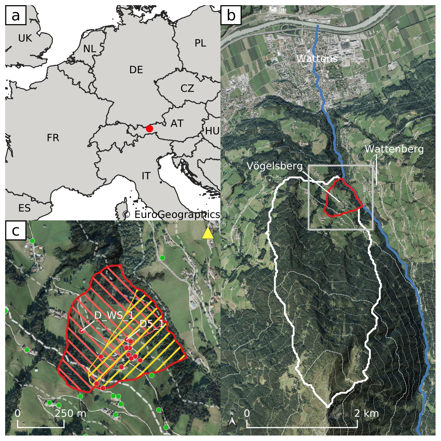
Figure 1(a) Location of Vögelsberg in Europe. (b) Overview of the landslide catchment (white) and active region of the Vögelsberg landslide (red). Dashed contour lines are shown every 100 m of elevation change. The coverage of sub-figure (c) is indicated in gray. (c) Detail of the active region of the Vögelsberg landslide. The northern subsection of the slope (red) and southern (yellow) section and overlapping area are marked. Out of a total 53 retroreflecting prisms, the 29 benchmarks with the longest time series (2016–2020) are shown. Benchmarks on the landslide are shown in red, stable, reference benchmarks in green. The time series of benchmarks “D_WS_1” and “D5_1” are shown in Fig. 2. The location of the total station in Wattenberg is marked by a yellow triangle (backgrounds: Eurostat/EuroGeographics; Federal State of Tyrol, Austria).
In 2016 a Leica TC1800 automated total Station (ATS) was installed in Wattenberg, opposite Vögelsberg, by the Division of Geoinformation of the Federal State of Tyrol. The system surveyed each of the 53 benchmarks every hour. Extensive corrections to the measurements were necessary, primarily due to the instability of the monument the total station is located on. In this study a series of pre-processed range measurements was used, fixed to stable benchmarks around the active area that showed no signs of landslide deformation damage. The accuracy of this time series was estimated to be in the order of ±0.54 cm yr−1 (Pfeiffer et al., 2021). The time series of the displacement rate at the two benchmarks used in this study are shown in Fig. 2; their locations are indicated in Fig. 1. The time series of the other benchmarks are shown in Fig. 3 of Pfeiffer et al. (2021).
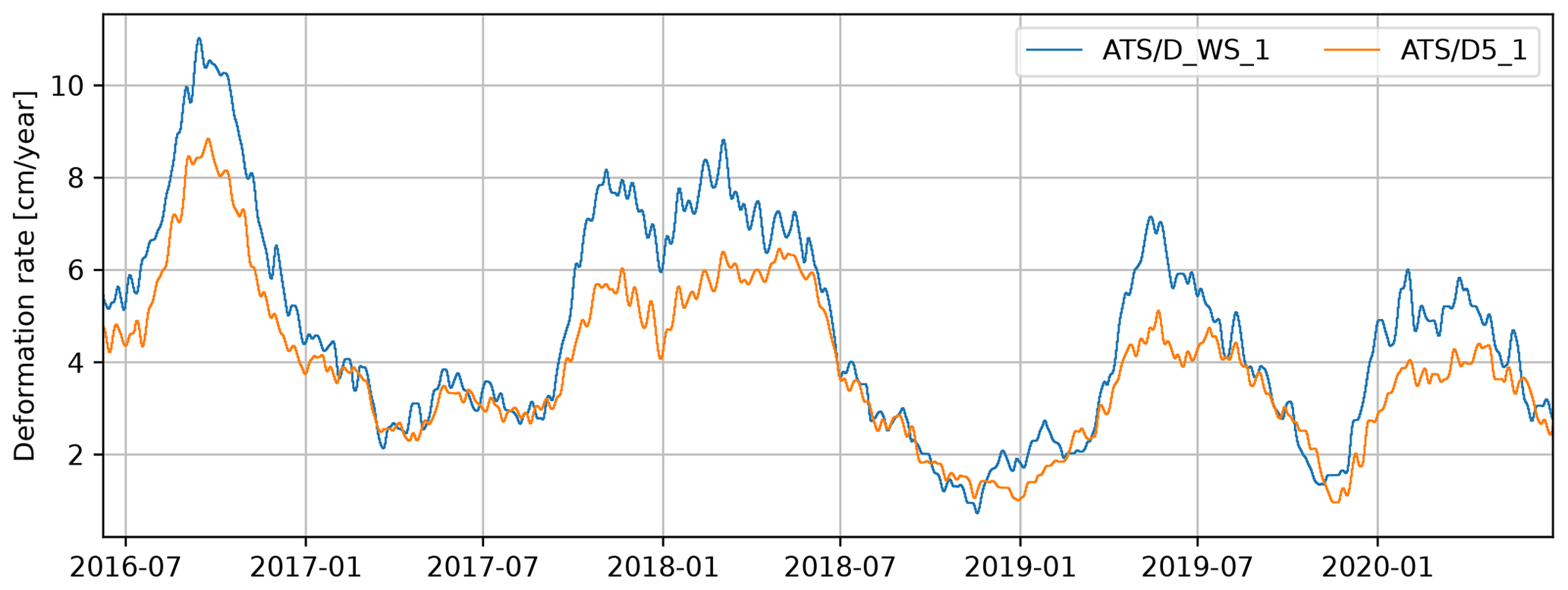
Figure 2Daily deformation rate of the Vögelsberg landslide at benchmarks “D5_1” and “D_WS_1” (Fig. 1), as measured by the automated total station and smoothed by a moving average filter over the last 32 d.
The deformation of the Vögelsberg landslide is a complex response to the hydro-meteorological conditions in the catchment, in particular precipitation and (delayed) infiltration from snowmelt. A binary prediction of stability/instability or acceleration/deceleration is insufficient for the Vögelsberg landslide, as the slope is undergoing continuous deformation. Pfeiffer et al. (2021) conducted a full, in situ assessment of the hydro-meteorological drivers and found a 20–60 d time lag between rainfall and acceleration and a 0–8 d time lag between snowmelt and acceleration. Noteworthy is the difference in behaviour between the northern and southern sections of the slope, represented by benchmarks “D_WS_1” and “D5_1” respectively (Fig. 2). The northern section of the slope (“D_WS_1”) shows a higher variability in the deformation signal, with stronger accelerations than the southern, inhabited section of the slope (“D5_1”). We focus on these two benchmarks as a balanced representation of the two landslide sub-systems.
The deformation rate, derived from the total station range measurements, was smoothed by a moving average filter until few, noise-induced, negative (up-slope) deformations remained, while maintaining the highest possible temporal resolution (Fig. B1). Only historic observations may be used in an operational early warning system, and a moving average of the most recent 32 d was necessary to remove most of the noise. As a consequence, the onset of acceleration will only be of the signal and thus severely dampened, stressing the need for an acceleration prediction rather than extrapolation of deformation measurements as a warning signal. Moreover, signals shorter than the filter length will be reduced in amplitude.
Our model's aim is to predict the landslide deformation based solely on the current conditions at the slope. No recent deformation observations or prior defined geomechanical model will be available to our model during prediction. The main model constraints are that we have a relatively limited number of data points (1482 samples) and will work with readily available remote sensing data and products. Furthermore, we set the objective to model with daily time steps and a forecast lead time of 4 d. A successful prediction of the deformation rate 4 d ahead will demonstrate the model's ability to predict a tipping point based on the environmental conditions (acceleration, peak, deceleration). Moreover, a 4 d prediction would give sufficient time for further investigation as part of an early warning system.
With these constraints in mind, a system was designed based on a parsimonious recurrent neural network. First, we will introduce the data available. Second, an overview is provided of the pre-processing applied to the input variables. Third, we provide the specifications of our model. Last, the training and validation of the model are discussed.
4.1 Model variables
The model variable selection is based on the analysis of factors of influence (Pfeiffer et al., 2021), and is mainly of a data-driven nature. Pre-disposing or causal factors, such as topography, that are necessary for a landslide to form are considered static in this study. Therefore, the focus is on the dynamic conditions leading up to landslide instability and deformation as well as triggering factors. The selection of variables is listed in Table 1.
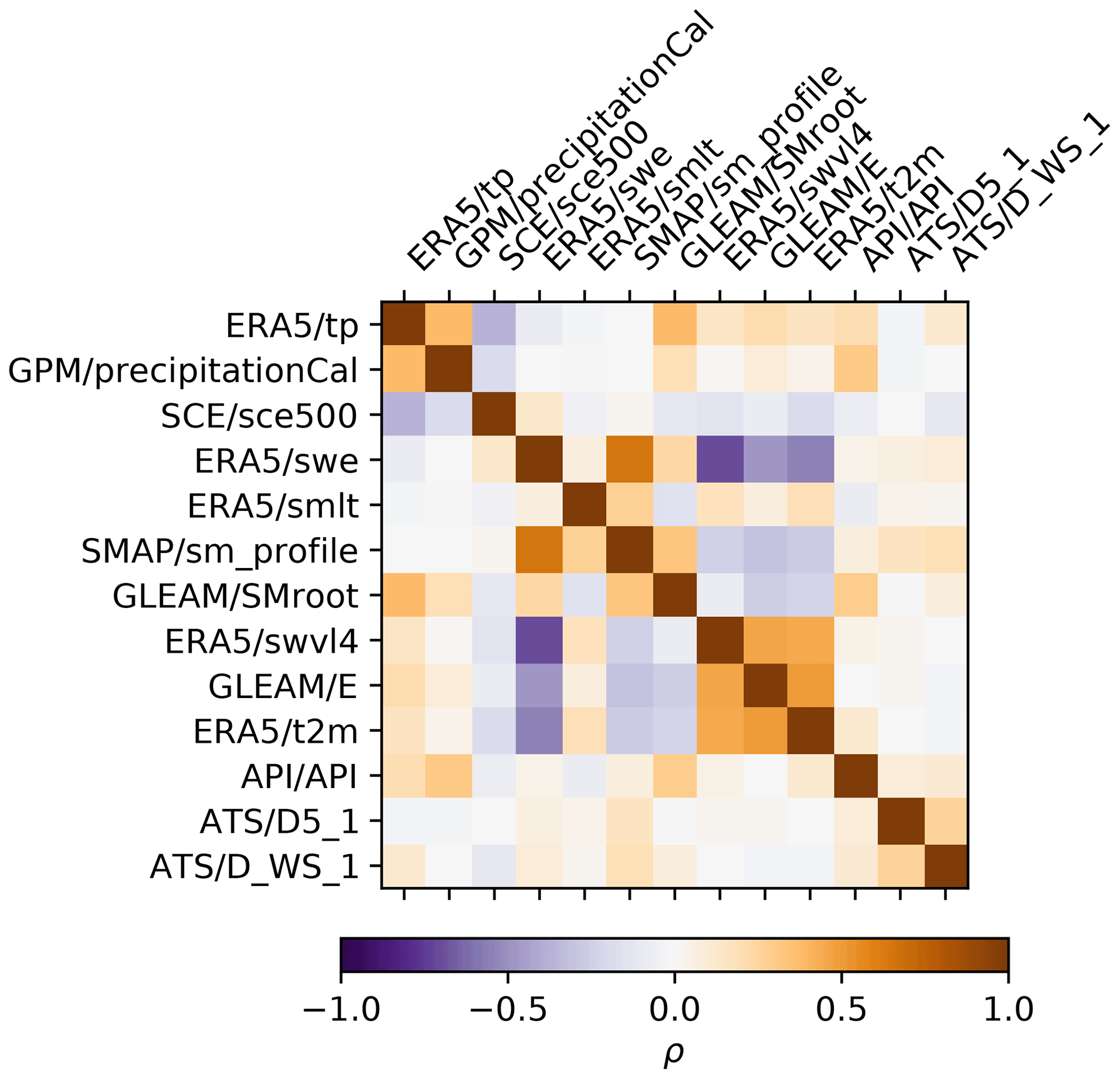
Our method is designed with the intent to be generally applicable. Therefore, except for the deformation, remote sensing products were used, as they are likely to be available elsewhere as well. Where available, redundant products that represent the same or similar quantities were included to assess their relative performance in the nowcasting model. The correlation between the products is limited (, , Fig. A1), indicating differences between the products of the same quantity. Effects that may not be observed directly, such as soil moisture under snow, require some form of modelling or reanalysis. These quantities, not directly available from remote sensing, are taken from reanalysis models “ECMWF reanalysis, version 5” (ERA5) and the “Global Land Evaporation Amsterdam Model” (GLEAM).
The desired output of our model is a daily, 4 d ahead prediction of the landslide deformation rate at benchmarks “D_WS_1” and “D5_1”. Reference, training, and validation samples are provided by the automated total station located on the Wattenberg, opposite Vögelsberg (Fig. 1). Deformation measurements were performed hourly from 4 May 2016 to 28 June 2020 and aggregated to 1482 daily averages to reduce noise. The noise in the signal was further reduced by a 32 d moving average filter, the results of which are shown in Fig. 2. The time series at the 51 other benchmarks (Fig. 1) were not used in the modelling.
Table 1Selection of time series considered for integration into the model. Deformation variables are marked “D”, while slope conditions, input variables to the model, are marked “V”. Observations are marked “S” for directly observed variables processed and available within the time frame of a nowcasting system, “R” for reanalysis variables, and “M” for variables modelled within this study (see Sect. 4.2). References to the various sources are provided in the main text. The internal identification is derived from the variable as referenced by the source and is used throughout the figures to refer to the various time series. From rasterized products, only the time series closest to Vögelsberg was used.
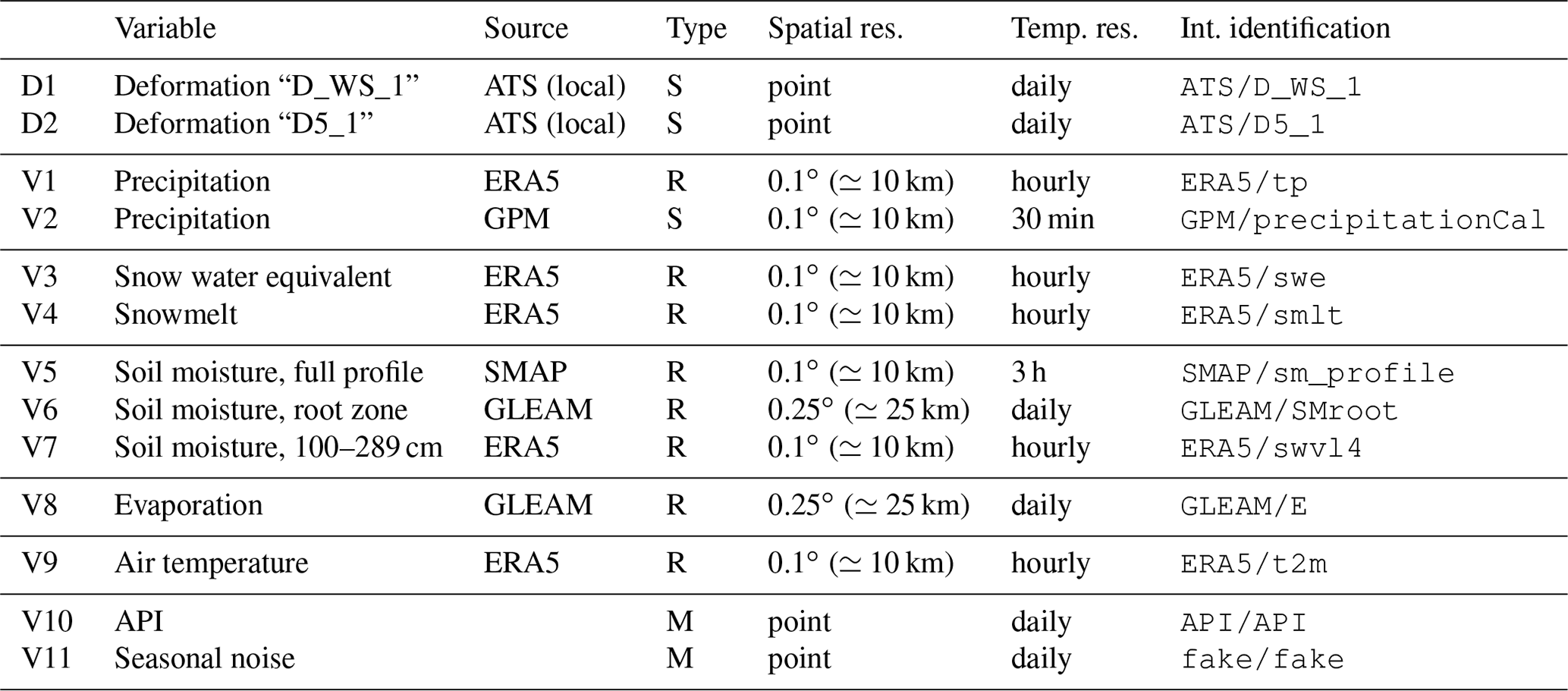
Daily precipitation information is provided by the Integrated Multi-satellitE Retrievals for GPM (IMERG) algorithm of the Global Precipitation Measurement mission (GPM) (Huffman et al., 2019). “Early” results are provided with sub-day delay and are therefore especially suitable for an operational nowcasting model. For comparison, daily precipitation from the ECMWF ERA5 Land reanalysis is included as well (Muñoz Sabater, 2019). Snow properties are covered by two products of the ERA5 Land reanalysis: snow water equivalent and snowmelt.
Soil moisture, especially at depth, cannot be observed directly from space at a high enough resolution for this application. The low-latency, operational products from the Copernicus Land Service, Soil Water Index and Surface Soil Moisture, are frequently unavailable either due to unfavourable slope topography or due to snow cover. Alternatives are provided by SMAP L4 (Entekhabi et al., 2010; Reichle et al., 2022), “Global Land Evaporation Amsterdam Model” (GLEAM) (Martens et al., 2017; Miralles et al., 2011), and ERA5 Land (Muñoz Sabater, 2019). Evaporation estimates are taken from GLEAM as well. Air temperature, a proxy indicator of evaporation and snowmelt, is included from ERA5 Land (Muñoz Sabater, 2019).
4.2 Variable preparation
The model is fed with the 11 variables defined in Sect. 4.1 (Table 1). Except for the deformation time series, all sources consist of gridded products with wide area coverage. In this study, only the data point closest to the active part of the Vögelsberg landslide was used. To match the time resolution of the deformation measurements, the model is run at daily intervals. Observations available at shorter intervals are aggregated to daily means first. Where data are missing, for example due to sensor failure, the values are filled with the data from the previous day (forward filling), as would be possible in an operational scenario. Furthermore, two modelled time series were added to the system: an antecedent precipitation index (API) as a basic hydrological model and a random, seasonal noise signal.
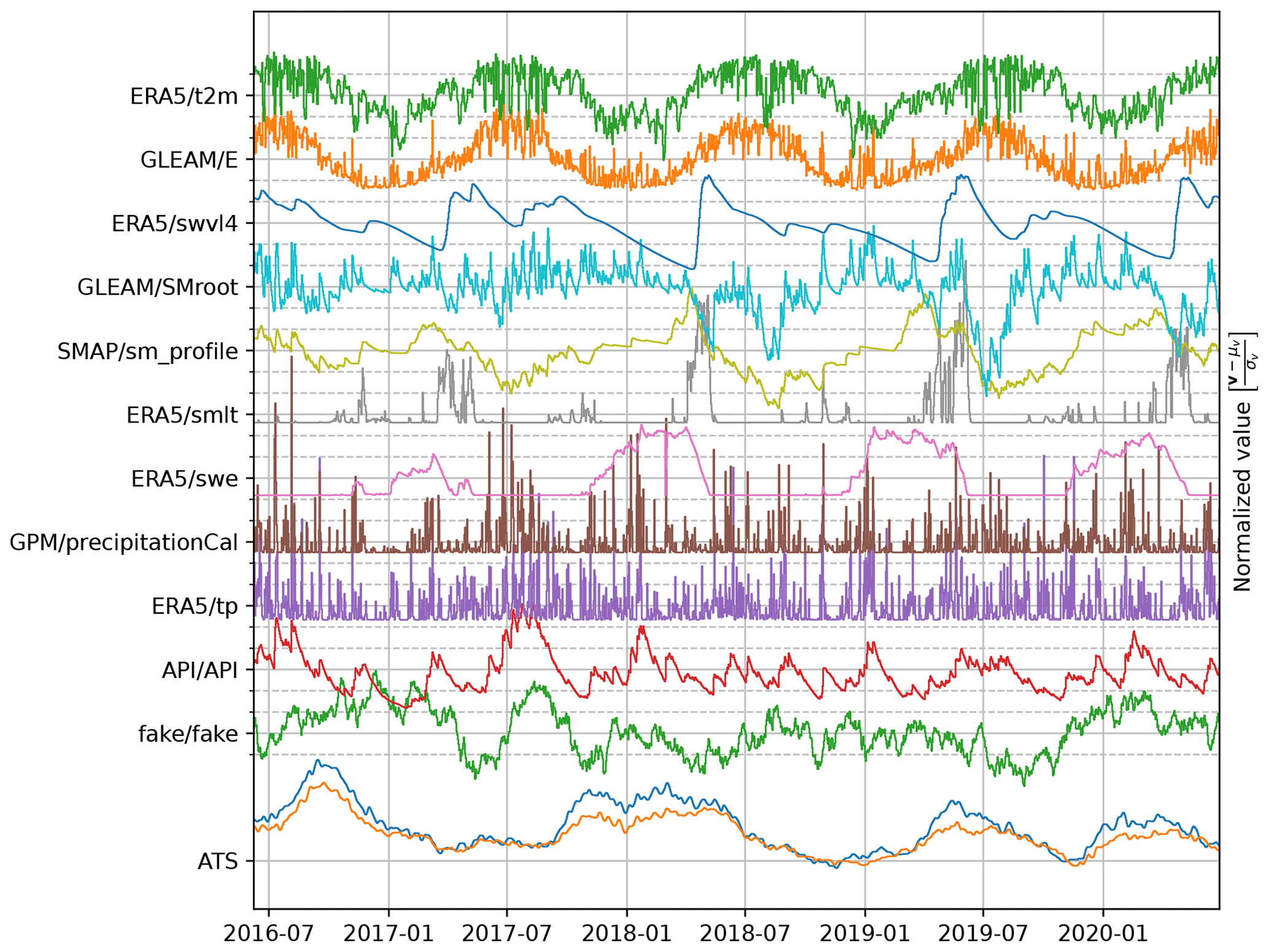
Figure 3Overview of the variable space (Table 1). The values are offset to a zero mean and scaled by their standard deviation. A single iteration of the seasonal noise (fake/fake) is shown as an example.
The antecedent precipitation index (API, API/API, V10) was designed to estimate the water present in the watershed (Kohler and Linsley, 1951; Heggen, 2001). The API is included to determine if such variable could support the deformation nowcasting model. Precipitation less than 0.1 mm was ignored, in addition a 10 % direct evaporation loss, and a 4 % daily storage loss is assumed. These parameters were chosen based on an estimate of the hydrological setting by an experienced landslide hydrologist. The API at time step t is calculated as
with p being the daily precipitation sum. The API, calculated from the operational GPM precipitation data (GPM/precipitationCal), is shown in Fig. 3.
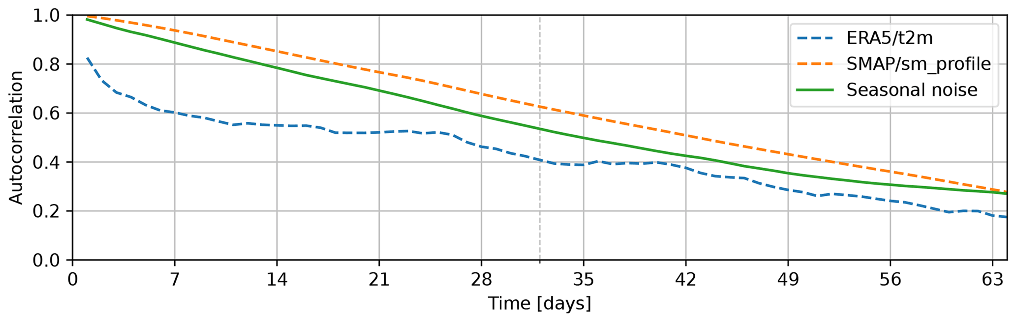
Figure 4Autocorrelation of one of the generated signals compared to the autocorrelation of the temperature as taken from ERA5 (ERA5/t2m) and the soil moisture estimate from SMAP (SMAP/sm_profile). The length of the history as used by the model, 32 d, is indicated by the dashed line.
A random variable with seasonal characteristics is added to the variable selection to analyse the effect of spurious correlation on the model. The random variable, fake/fake (V11), based on Brownian motion is tuned to match a typical seasonal characteristic in the 32 d history relevant to the model. The auto-correlation behaviour is illustrated in Fig. 4 and resembles the dynamics of both the surface temperature as provided by ERA5 and the soil moisture from SMAP for the first 2–3 months. Longer correlation periods are not relevant for our model.
All variables are offset to become zero-mean and scaled by the standard deviation. Therefore, all input variables are on approximately equal scale and represented as deviations from their average condition. The normalization parameters, mean and standard deviation, should be kept fixed while new data are added to remain consistent with the scaling of the time series used during training. The data set is fed to the model as a time-stamped collection of daily observations, illustrated in Fig. 3.
4.3 Model configuration
Our model is a shallow neural network with only a single hidden layer (Jain et al., 1996). This hidden layer consists of a single long short-term memory (LSTM) node (Hochreiter and Schmidhuber, 1997) that resembles a bucket model for the water storage in the subsoil. The model is supplied with a 32 d history of observations, equal to the length of the moving average filter, longer than the lag time for snow (0–8 d), and sufficient to cover most of the 20–60 d lag time for rainfall at the Vögelsberg landslide found by Pfeiffer et al. (2021). From a predefined, optimized initialization, the model is cycled for each day of preceding observations, feeding the observations into memory before a prediction is made based on the final bucket values (m). The model is illustrated in Fig. 5, as function of environmental conditions (x, Table 1), at each of the n=32 d preceding the nowcast, the LSTM node and four neurons of a single benchmark, one for each prediction day. This last, output, layer is repeated for both benchmarks (“D_WS_1” and “D5_1”) to be predicted, while the LSTM memory (m) is shared between the benchmarks to reduce the number of parameters.
In total, for a network configuration with a single memory cell (m), 68 parameters have to be estimated. The LSTM node, with one hidden state, requires 52 parameters to be estimated for the 11 variables (Table 1). A total of 16 parameters are required for the output, eight for each of the deformation time series: one bias and one scaling parameter per day for the final state of the LSTM node. The number of parameters to be estimated is independent of the history length.
Four parameters are added per extra prediction day (two benchmarks, one bias and weight each). An extra memory cell requires extra parameters, with h the current number of hidden nodes and x the number of input variables, while only four parameters are added for each additional input variable. Hence, extra memory always requires more parameters than extra input variables. Therefore, to limit the number of parameters in the model and minimize the risk of overfitting, the addition of a variable to the model should be preferred over the addition of a memory cell.
An interpretation of the network is that the development of the slope state in the last 32 d is described by the LSTM node. The state is scaled, and otherwise matched to the individual benchmarks, by the output neurons. The 4 d are an extrapolation of the current state of the system; no prediction of the conditions on the slope is made.
The “mean squared error” was chosen as the loss function. This function that quantifies the difference between the predicted and observed deformation is to be minimized during training. The quality of the prediction is measured on the period not used for training. This function assures that the cumulative deformation over time is realistic, as errors are balanced between overestimation and underestimation. Therefore, the predictions will not show a bias towards acceleration or deceleration. The TensorFlow machine learning framework was chosen to implement the model (TensorFlow Developers, 2022). The LSTM model is implemented in a stateless fashion: the warm-up phase is repeated for every nowcast. The model was run on a workstation based on an Intel Xeon W-2123 (4 cores, 8 threads, 3.6 GHz) with 32 GB RAM, while model variations were tested on the high-performance computing cluster of the Delft University of Technology. Given the limited size of the region of interest, as well as the limited number of parameters, the full model fits into 1 GB of memory.
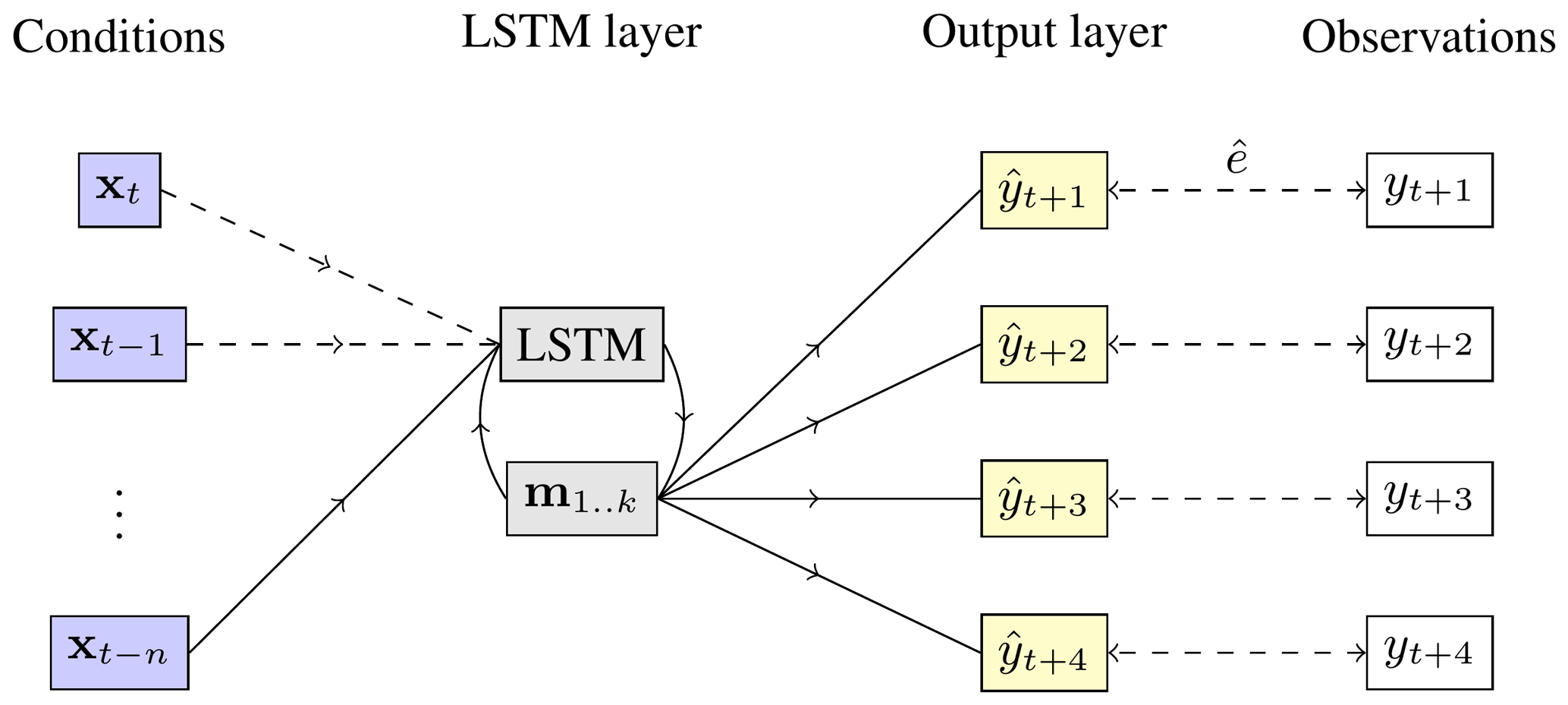
Figure 5Simplified schematic of the model. From left to right: the hydro-meteorological conditions (xt) on the slope at the current (t) and n preceding time steps; the LSTM layer, including its internal feedback and memory cells (); the output layer , which combines the k memory cells m of the LSTM node to four predictions; and the observations yt, as available for comparison during training and validation. During initialization, the conditions on the slope are fed to the system on a day-by-day basis, starting at the oldest observations. The output layer is only invoked at the last iteration, with the final values of the LSTM memory. The parameters of the LSTM layer are optimized on both deformation time series in parallel, the output nodes are tuned individually for each benchmark.
4.4 Model training and validation
During training the model parameters are tuned such that the final model state best describes the deformation prediction. The model is optimized with the Adam optimizer (Kingma and Ba, 2014). The model is trained on the loss; after 50 training passes that do not lower the mean squared error over the training period, the model's parameters are fixed. If this steady state is not achieved after 25 000 passes, the training is stopped anyway and the model parameters used as-is.
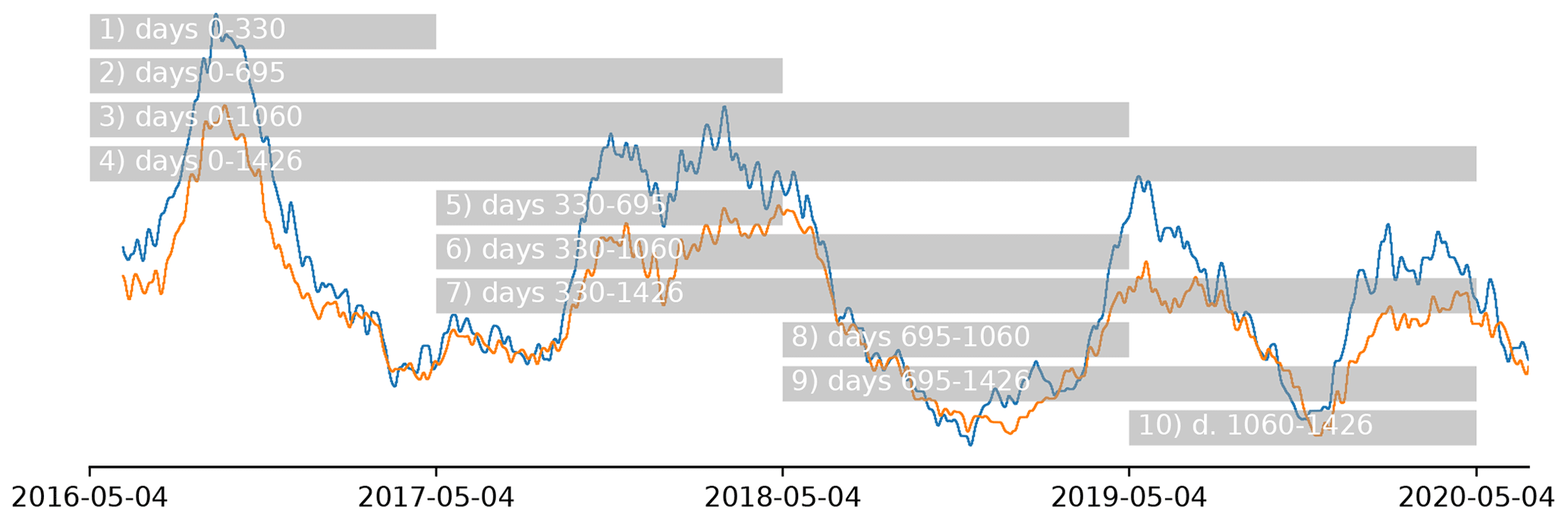
Figure 6Training periods as supplied to the model. The data outside the training period are used for validation. Note that with the longest training period (4) there are very limited validation data left. The deformation pattern (Fig. 2) is shown in the background for reference. As there is no clear seasonality in the deformation signal, the data set was split in approximate years from the start of the measurements.
Due to temporal correlation, training and validation cannot be divided over random chunks or batches according to the “traditional” 30 %–70 % chunks (Gholamy et al., 2018). Therefore, the training data are split into equal years instead, as shown in Fig. 6. Data outside the training period are used for validation. This includes the period before the training period, when available.
The robustness of the model to the selection of the training data is assessed from the stability of the results when training over the subsequent periods (Fig. 6), a variation on cross-validation (Krkač et al., 2020). Each model iteration starts with the same (random) initial weights but is trained independently from the start. The quality of fit is assessed by evaluation of the loss function, the mean squared error, on the periods not used for training. Finally, the model performance is compared between the training periods. Large deviations of the model quality suggest there are dynamics the system is not capable of describing.
To assess the impact of irrelevant data on the system, as well as the effect of overfitting, the additional, correlated random variable (fake/fake) is used. Overfitting will make the model prone to spurious correlation with this variable, which results in poor performance in the validation stage. Furthermore, to ensure there is no accidental correlation between the seasonal noise and the deformation signal during training and/or validation, the signal was re-rendered for every model run.
All possible combinations of the 11 input variables were tested on the model. With 11 variables this results in combinations, as each of the time series may be used or not (2 options), except for the case where no input is used. Furthermore, the model was trained and validated on each of the 10 combinations of training and validation year(s). Each sequence of model training and validation was repeated at least three times, to account for the `luck' introduced by the random initialization of each model. In total, 147 984 model runs were performed.
The best solution out of all model runs, judged on the minimal mean squared error on validation, is based on a single LSTM node and only 4 of the 11 input variables available: precipitation from GPM (V2), soil moisture from SMAP (V5) and ERA5 (V7), and evaporation from GLEAM (V8), where the numbers refer to Table 1. The minimal mean squared error on validation was achieved when the model was trained over period 3 (Fig. 6, 4 May 2016–4 May 2019); the mean squared error of this model run was 1.03 cm2 yr−2, below the average of 3.15 cm2 yr−2 (σ≈1.3 cm2 yr−2, from 1718 samples) for this model configuration.
The full nowcast is shown in Fig. 7, including the training period shaded in gray. Although, based on visual inspection, reasonable results are achieved in summer and autumn; the nowcasting model is unable to predict the deformation rate in winter and spring in the training period. Especially surprising is the jump in the winter of 2018/2019, where a strong acceleration is predicted which does not occur until early summer. The validation period, from May 2019 onwards, shows little variation. The deceleration in the summer and autumn of 2019 is overestimated and shifted; likewise, the acceleration in the December 2019 is predicted correctly but too early. Overall the predictions show long-term stability (Fig. 8) as enforced by the choice of the mean squared error as loss function.
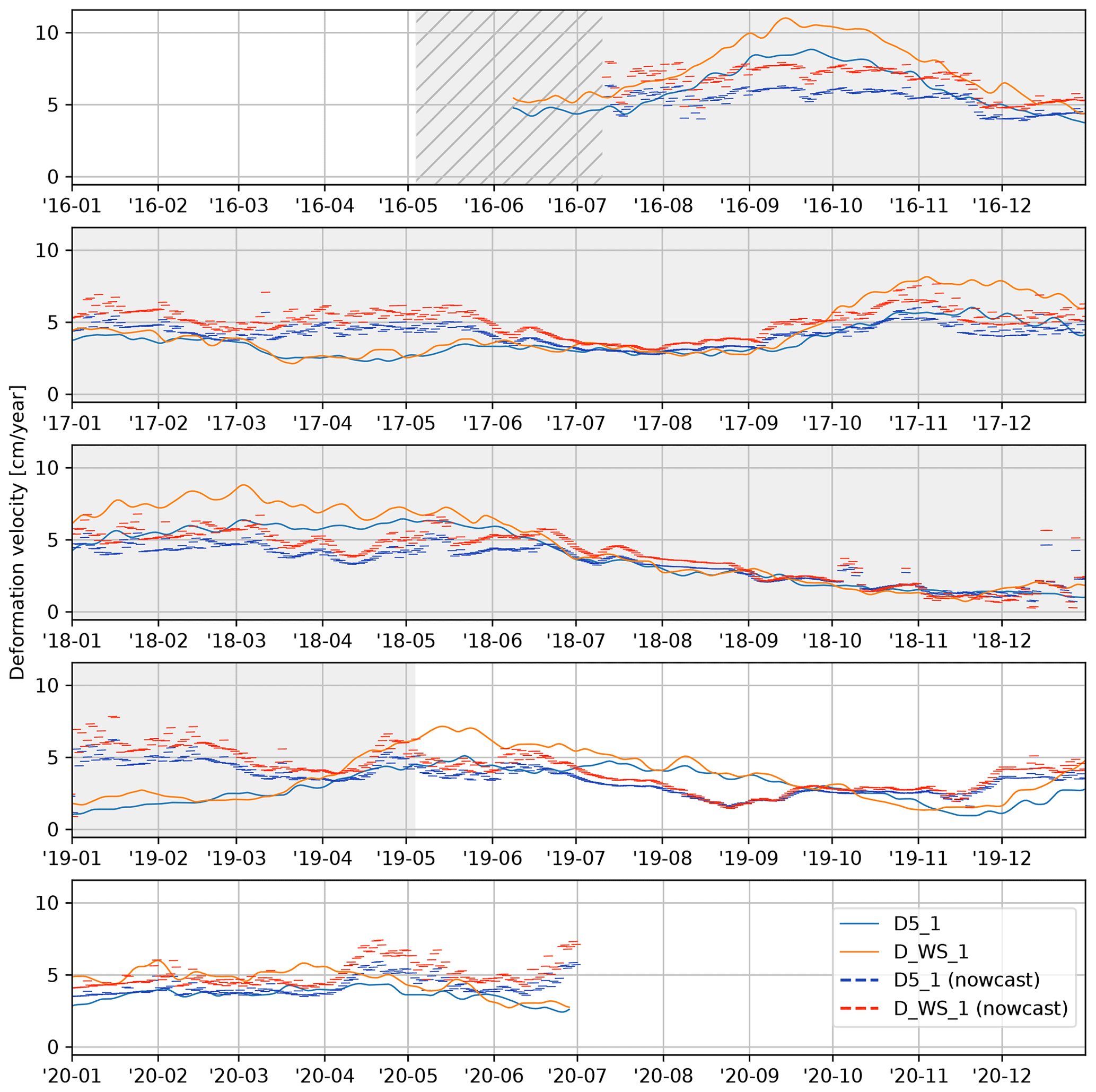
Figure 7Result of the deformation nowcast, run of the full time frame of the available deformation time series. The shaded time span was used for training. Shown as thin lines are the subsequent, daily, nowcasts for benchmarks “D5_1” and “D_WS_1”. Per day, four deformation nowcasts are shown, with the start of each line being the day after the day the nowcast was issued. Note the warm-up time at the start, shown hatched and without predictions, that is required to initialize the moving average filter on the deformation data and fill the memory of the LSTM node. The final nowcast ends 4 d after the end of the reference measurements.
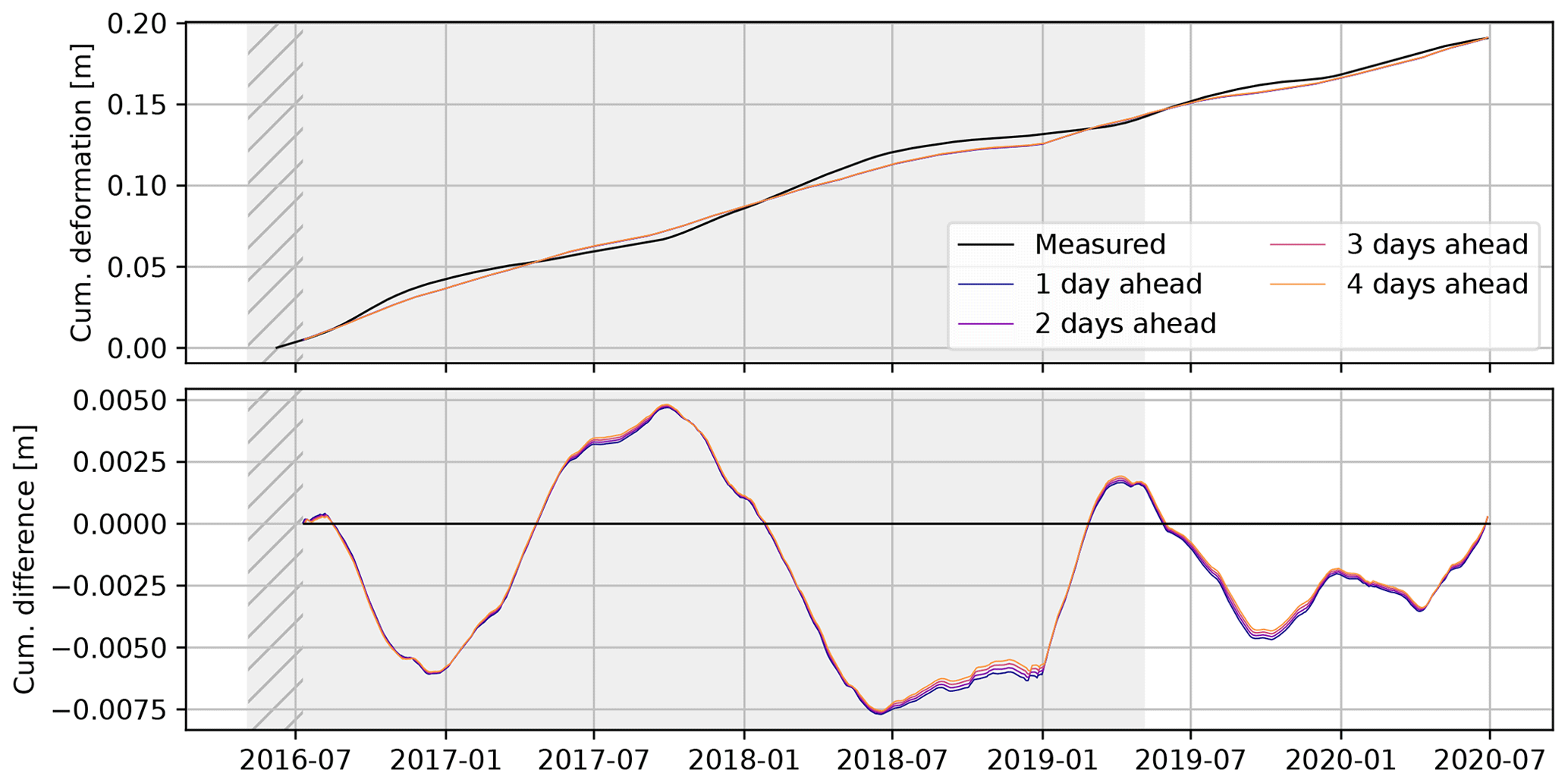
Figure 8The cumulative deformation, as predicted by the consecutive, individual model runs closely matches the observed deformation over the full 4 years of deformation measurements. The difference is calculated as “modelled − observed” () cumulative deformation. The training period of the model is marked in gray; hatched are the warm-up periods of the moving average filter and memory of the model.
The modelling results are overall unsatisfactory: the acceleration and deceleration are typically not predicted timeously or at all. This is surprising in light of the success reported by others (Table C1). Although we designed our model to match our understanding of the interplay of hydro-meteorological conditions and deformation, the physics behind slope processes at the Vögelsberg landslide, the model was unable to capture this relation. The deformation at Vögelsberg is driven by a complex interplay of hydro-meteorological conditions, unlike most of the examples in Table C1, that often includes a strong, stable driver, such as a reservoir. This lack of such a single, strong driver complicates the working of our data-driven model.
5.1 Contribution of individual variables
Due to the complexity of the operations applied to the input signal in the LSTM layer, it is not straightforward to analyse the contribution of the individual components to the final model outcome. As all model variations were tested (Sect. 4.4), it is possible to analyse the influence of the presence of a variable by comparing the quality of the model variations. For this analysis, only model iterations with a training period (Fig. 6) that left at least 1 year left for validation were used. Furthermore, all model variations were run multiple times to assess the robustness of the outcome to the random initialization.
Figure 9 shows the results of this analysis and illustrates the mean squared error over the validation period for all models including each variable. For each variable the minimum and average mean squared errors for the validation period are shown, while the maximum mean squared error is often out of range. The thickness of the line indicates the density of results for that mean squared error, where thicker lines at lower mean squared errors indicate a concentration of models with a high quality of fit.
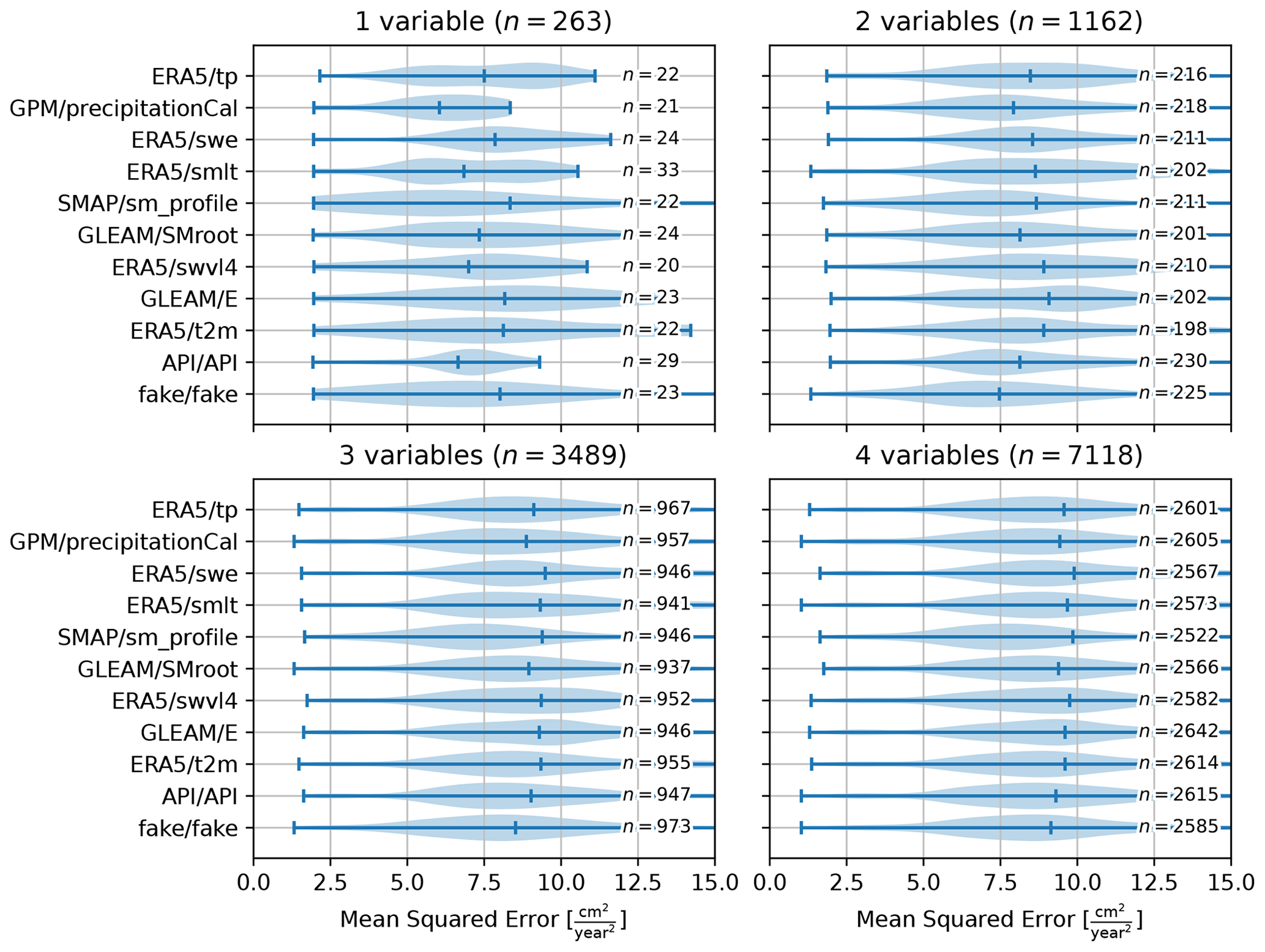
Figure 9Violin plots of the mean squared error for model variations with one to four variables, including the variable listed. For more than four variables the relative importance of the individual variables to the model quality becomes insignificant.
Models based only on SMAP/sm_profile (V5) score the poorest (highest mean squared error) on average but with the widest distribution, including many solutions with a low mean squared error. The difference in performance between the variables vanishes as more variables are introduced into the model; however, the models including the SMAP soil moisture (V5) time series show a consistently larger range in performance, including models with a low mean squared error. Remarkable is the approximately equal performance between API/API (V10) and fake/fake (V11), where the latter contains no information on the hydro-meteorological processes and is only marginally outperformed by the antecedent precipitation index (API, V10). For models with more than four variables, there is no significant difference in model quality for any of the variables.
We believe the unsatisfactory performance of the model has three root causes: (i) the inability of the model to capture the complex dynamics of the system; (ii) the limited quantity of training data available to this type of problem; and (iii) the limited, noisy representation of the slope dynamics in the available remote sensing data. Most natural deep-seated landslides are characterized by a complex interplay of causal (antecedent) and triggering conditions: this is also true for the Vögelsberg landslide. However, we believe that it is exactly these challenges that we should aim to tackle with a machine learning model approach.
6.1 Model configuration
The possibilities for data-driven modelling are infinite: our model is only a single realization of the possible combinations of variables and operations. This raises three questions regarding the model selection: (i) how to match model and process, (ii) how to validate and quantify the quality the nowcast, and (iii) how to tune the model implementation.
The major challenge for the model of a deep-seated landslide is the discrepancy between the sub-daily variations of the input (especially precipitation and snowmelt) and a delayed, daily output (accelerated deformation). Therefore, non-time-aware models show erratic behaviour, as the consequence of sudden changes to conditions such as snow cover and (extreme) precipitation that, in reality, do not translate into immediate acceleration. Traditionally, the addition of groundwater physics, smoothing the hydro-meteorological signal, circumvents these peaks. However, the addition of groundwater physics requires knowledge of the geohydrology of the specific slope.
An LSTM node resembles a bucket model and was chosen to capture the delay between precipitation and deformation by modelling the buildup of water in the model. Our results showed that our model was unable to fully capture these hydro-meteorological dynamics. For reference, five alternative models were implemented (Table 2) that were designed to better address the diversity of the slope, and/or lower the number of parameters required by the model to prevent overfitting.
Table 2List of reference models tested for comparison to lstm1-32. Their performance is shown in Fig. 10. To calculate the number of model parameters, n is the length of the time series provided to the model, k is the number of input variables, m is the number of memory cells, and h is the number of hidden nodes. A single hidden layer is assumed. The number of parameters includes the final, output layer of four nodes for each of the two deformation time series.
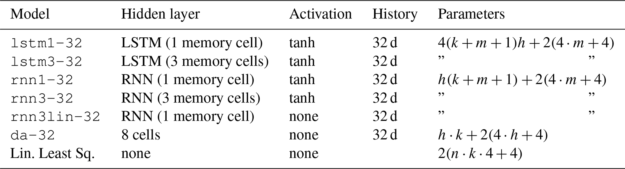
The lstm3-32 model contains two additional memory cells (buckets) in the LSTM node compared to the lstm1-32 model previously used. The concept is that the memory cells may represent different systems or layers in the subsurface, potentially interacting with each other. For each subsequent time step, all states are included in the calculation of the new states and could therefore also model interactions between layers in hydrology, such as the transfer between layers.
The rnn1-32 and rnn3-32 models based on a traditional recurrent neural network are similar to their LSTM counterparts, with one and three memory cells respectively. However, unlike an LSTM node, they are unable to “forget” their state on command, and are more susceptible to unstable behaviour. The rnn1lin-32 did not incorporate an activation function and is comparable to a moving average filter with interaction between the variables. For all three models the number of parameters is less than for the equivalent LSTM-based models.
The da-32 model resembles a linear least squares model. Variables are first summarized as their average over their 32 d history and included in eight nodes without bias in the hidden layer of the network. The final predictions are a linear combination of the node values. In a “traditional” linear least squares solution, a direct combination of all input variables, the number of parameters will often outnumber the number of observations available and were therefore not tested.
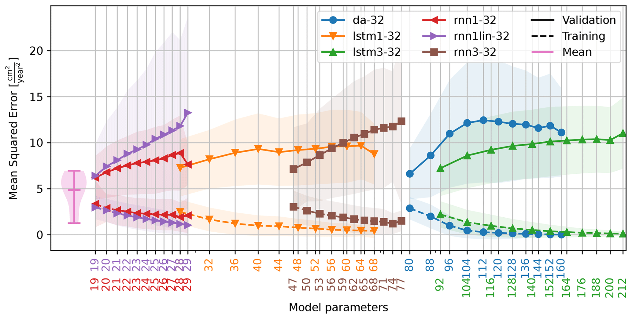
Figure 10Relationship between the number of model parameters and the quality (mean squared error) of training and validation as extracted from the 147 984 model runs. The number of parameters is related to the number of input variables. For LSTM-based networks, for example, there are four parameters per input variable per LSTM memory cell required. Note the logarithmic scale on the x axis. On the left, the distribution of the mean squared error of a reference model is shown. In this model the mean deformation rate was determined over each of the nine training periods (Fig. 6) and used as a “predictor” for the remainder of the time series.
The performance of each model is shown for comparison in Fig. 10 as a function of the parameters required. Model performance is typically optimal for models with only a single parameter and is comparable between the models. Like the original model (lstm1-32), each model was re-run multiple times with a random initialization of the seasonal noise (V11) and model parameters to verify the consistency of the output. Most alternative models do not outperform the average deformation rate as predictor for the future deformation rate, as shown in Fig. 10.
6.1.1 Performance metric
For early warning systems, prediction of the onset of acceleration (Fig. 11) is more important than the deformation quantity. However, false alarms, triggered by insignificant accelerations, may undermine confidence in the early warning system. At this stage of development, we would rely on professional interpretation by an expert to limit the number of false alarms. However, the system should warn the expert of potentially bad predictions, for example due to previously not encountered conditions. The timing of the nowcast should allow for further analysis of the prediction without jeopardizing precautionary measures for accelerated deformation.
This leads to five desired properties for the nowcasting system: the system should (i) predict onset of acceleration, (ii) predict the maximum deformation velocity, (iii) predict 4 or more days ahead that deformation will begin, (iv) predict when the slope is “stable” again, and (v) quantify the certainty in the prediction. Unlike most estimation problems, not only is the quantity of the predicted deformation important to the user but so is its timing. An acceleration phase predicted too early or slightly late may still trigger the desired alertness and still serves a purpose, even though the predicted amplitude on that day is wrong.
A “standard” error metric, e.g. the mean squared error, is sensitive to the mean as local optimum but is unbiased and therefore stable in the long term. As an alternative, such an error metric could be evaluated at “peaks and valleys”, the peaks of the deformation rate, only, emphasizing extremes and disregarding their onset. With this method there are less samples, only the extremes, but they are less correlated and include the amplitude of the event. Although this captures the timeliness of the extremes, it disregards the timing of the onset and pattern of the acceleration phase. Moreover, this approach requires information on the peaks and valleys and that those are correctly identified beforehand.
Due to the lack of information on the extremes of the deformation, we chose to use the mean squared error as the error metric. This metric ensured a long-term stability and connected stability of the deformation nowcast, as demonstrated by the cumulative deformation (Fig. 8). As a consequence, the system preferred “average” solutions, overestimating the deformation rate in stable periods and underestimating the deformation rate in periods of accelerated deformation. For reference, the mean deformation rate was determined over each of the nine training periods (Fig. 6) and used as a “predictor” for the remainder of the time series. This constant deformation rate “model” outperforms many of the more parameter-heavy models over the validation period, and its mean squared error is shown on the left of Fig. 10.
Accelerations of the Vögelsberg landslide are known to be triggered by precipitation in summer/autumn and by snowmelt in winter/spring (Pfeiffer et al., 2021). Simple models, based on a limited number of variables and/or with limited modelling freedom, may not be able to cope with both driving forces. As a consequence, their overall performance will be poor. The overall performance, however, does not reflect the performance per season or acceleration trigger. Therefore, to make such model behaviour explicitly visible, seasonal differences in performance could be included in the evaluation of the model's performance, for example by evaluating a model's performance metric per season as well. Training the model per season, however, will require sufficient, dynamic training data to be available over each season, severely reducing the length of time series available.
6.1.2 Derived variables
Additional variables may be derived from the direct observations. In our model, the antecedent precipitation index (API) is such a derived observation and was chosen to enhance the information content of the hydro-meteorological observations to the model (i.e. provide higher predictive power to the model). This “feature generation” is an important component of more traditional machine learning techniques, where the system is not expected to derive those relations autonomously. Derived, additional features were extensively used by Krkač et al. (2020, 2017), for example, who created additional features to capture the conditions on the landslide, or Miao et al. (2022), who derived 10 features from only two sources (rainfall, reservoir level). A drawback of the addition of large quantities of such derived variables to the system is that each additional time series requires additional model parameters to be optimized.
6.1.3 Handling unencountered conditions
Given the limited availability of deformation measurements, most of the data are required to train the model. Moreover, the variation in conditions is limited to the variation in those 5 years. It is therefore likely that the model will encounter conditions in operation that it had not encountered before. Due to the continuous nature of the model proposed, and the alternatives discussed in Sect. 6.1, the output for such conditions is not bound to the previously encountered conditions.
For simple combinations of variables, i.e. of a single or a few variables, the response may be tested empirically. Note that the full 32 d history has to be included in this simulation. However, the response may not be so straightforward: a warm summer day combined with hail from a thunderstorm may trigger an unrealistic “path” in the model. Therefore, for more variables, the number of potential combinations increases drastically and may no longer be feasible to simulate.
Predictions of extraordinary responses are not necessarily undesirable; an unbound acceleration, i.e. landslide collapse, prediction should be possible. However, the model would preferably warn for a potential unstable state of the nowcasting system. This could be achieved by an ensemble of models, either based on the same model, or model variations. Models with different time series lengths, especially, may be able to help pinpoint the source of the discrepancy.
6.1.4 Spatial distribution
Our model of Vögelsberg is based on two benchmarks that are on two distinct sections of the slope (Fig. 1) that have been shown to exhibit different deformation behaviour. The southern, inhabited part of the slope exhibits constant deformation, with limited acceleration in wet periods. In contrast, the benchmark on the northern part of the slope shows strong acceleration and deceleration as a delayed response to strong precipitation (Pfeiffer et al., 2021). Although our models are unaware of this spatial relationship, it is found empirically during training, as the shared LSTM node, representing the slope processes, is weighted differently for each benchmark.
As an alternative, a location index could be specified, for example as a binary indicator of the landslide section or as continuous signals such as the distance to the centre. Instead of two or more predefined outputs from the same model, a single model may handle different benchmarks differentiated by additional input variables encoding their position within the system. However, given the shallow model design, care should be taken to design the model such that this index works as a scaled multiplier of the hydro-meteorological conditions.
6.2 Limited number of distinct events
Over the full time span of the measurements, four distinct acceleration periods can be identified (Fig. 11). These acceleration periods are especially of interest to an early warning system, as they mark the start of a period of accelerated deformation and associated hazard. Although the periods of accelerated deformation are comparable in length to the periods of continued, but reduced, deformation, the acceleration events are much shorter (Fig. 11). Therefore, these periods are underrepresented in error metrics during training and validation. However, training on these four periods alone leaves insufficient variability to describe the system and reliably fit the required model parameters. Furthermore, the episodic deformation behaviour poses a challenge to the prediction system, since the forcing variables on the slope do not reflect such sudden changes observed in the deformation behaviour, as shown in Fig. 3.
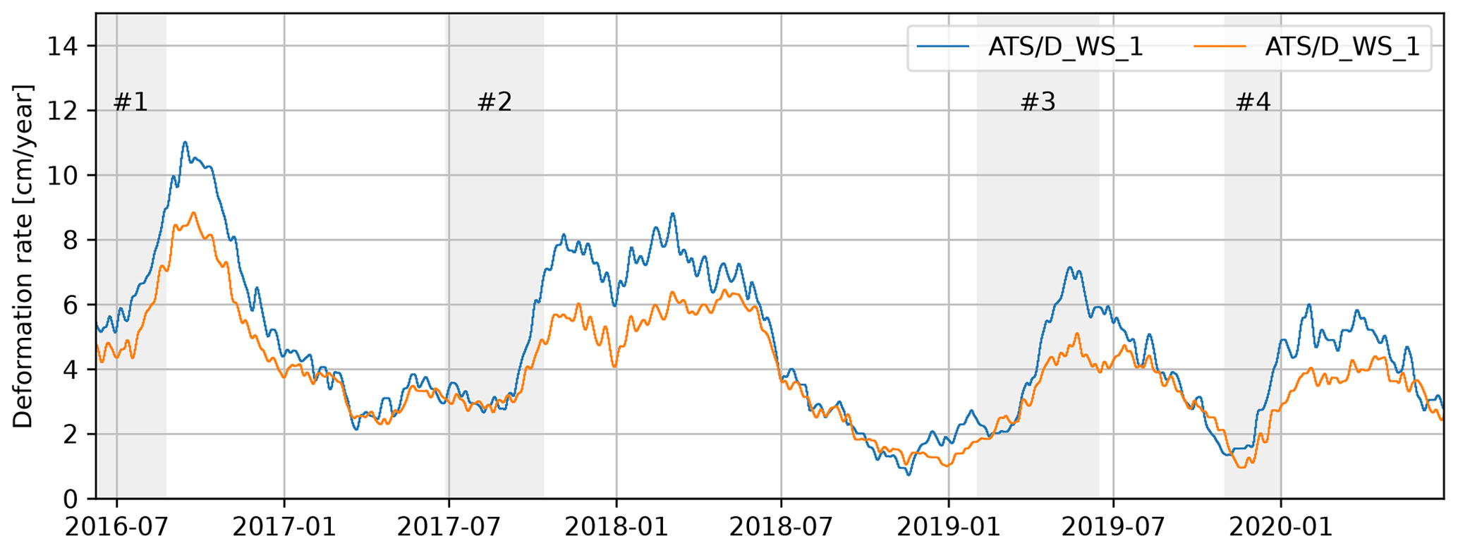
Figure 11Three acceleration events (#1, #2, & #3) at the Vögelsberg landslide, as identified by Pfeiffer et al. (2021). The fourth acceleration period (#4) was identified in the data acquired after Pfeiffer et al. (2021).
6.2.1 Length of training
Given that there is more than a single degree of freedom in the model, without prior knowledge of the process, there is no predictive power in a single acceleration event. Hence, multiple events are required to properly train complex models in the absence of constraints on the process and model. As a consequence, due to the limited variety of events in the training data, the predictive power of the nowcasting system may be reduced due to overfitting on the characteristics of these events only.
To test the effect of the training length on the models, the models were trained on 9 of the 10 training periods identified in Fig. 6 that had a least a year left for validation. The mean squared error, measured on the training as well as validation period, is shown in Fig. 12. The results are consistent between the models: all models show that as the training period increases, the quality over the training period decreases (dashed line, increasing mean squared error) due to the increased variability of the events therein. Likewise, the quality over the validation period increases (solid line, decreasing mean squared error) as the model generalizes better. This is also reflected in the lower standard deviation for validation over longer training periods. Hence, a longer training period makes the system more robust against the variations encountered by the system. To train and validate the nowcasting system, the time series was subdivided in calendar years measured from the start of the measurements. An alternative, common subdivision would be in hydrological years or water years that are typically defined to be from 1 October to 30 September and divided by the precipitation minimum (Lins, 2012). This subdivision is typically applied to cut the data in a hydro-meteorologically quiet period of the year. However, the strong deformation events in period 1 and 2 overlap with this subdivision. Furthermore, with this subdivision, only three periods would be available instead of four. Moreover, Parajka et al. (2009) show that the period of minimum precipitation cannot be pinpointed to a single winter month. Therefore, the decision was made to align the training years with the measurements instead.
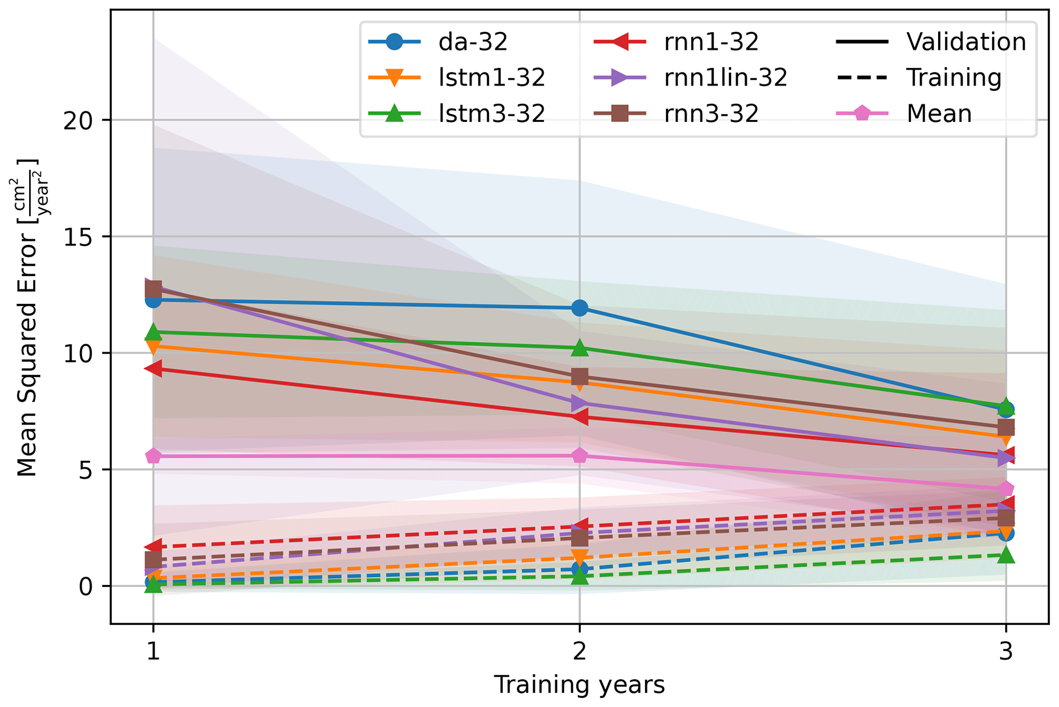
Figure 12Length of the training region, aggregated to (approximate) years, compared to the quality of fit of the model, measured as the mean squared error. An increase in model fit is visible with the increase in training length; however, most models are outperformed by the models that use the mean deformation rate (pink) of 1, 2, or 3 years respectively as the predictor.
6.2.2 Noise reduction of the deformation signal
Essential to the success of the nowcast are the properties of the signal to be predicted. The effect of noise in the deformation signal on the modelling is twofold: first, random perturbation complicates the training by masking the best solution, and, second, this leads to an underestimation of the final quality of the model during validation. Hence, the noise in the deformation signal defines the upper limit for the quality of the deformation estimate. Up-slope deformation, present in the raw deformation time series, was considered to be unrealistic and therefore noise by definition. Under the assumption that the noise is unbiased, the noise will be reduced in averaged samples. Therefore, a moving average filter was applied to the deformation time series with increasing length until no negative deformation remained.
The model was developed with the requirements for an operational system in mind, restricting the system to only use historic observations at any point in the process. The inclusion of future samples would require the system to react to future conditions that have not (yet) been observed on the slope: any filtering, such as smoothing, should not drag future observations back in time. Therefore, the moving average filter cannot be centred, and averaging is applied to the preceding 31 d rather than ±15 d around the current time step as would be possible in reanalysis.
The variation in the deformation signal at Vögelsberg is relatively small, in deviation from a long-term trend. Due to the millimetre-scale measurement uncertainty in the deformation measurements, the deformation signal is dominated by noise on the short timescale of days to weeks, and the relevance of a deformation prediction on a daily basis is doubtful. Furthermore, due to the inertia of the landslide body, as well as smoothing of the deformation measurements, accelerations and decelerations are spread over adjacent days (Fig. 6), and the amplitude of the acceleration is lost. For a successful, daily application, a clear separation between events and noise is required (higher signal-to-noise ratio), either due to a faster process or due to reduced noise in the deformation observations.
6.3 Input variables
The variable selection in Table 1 was compiled based on our knowledge of the physics behind the landslide process, as well as the availability and continuity of the data. With the ambition for a future, regional implementation in mind, the variables preferably come from satellite remote sensing observations rather than local, field sensors. However, we did not succeed in a fully remote-sensing-driven operation due to the limited availability of such operational products. Especially deformation observations from space (satellite radar interferometry, InSAR) were found to be promising, but we were unable to replace our local deformation time series with the noisier satellite deformation data.
6.3.1 Availability of variables
The model was designed under the assumption that data from all sources are continuous and readily available to the system. Out of the variable selection (Table 1), only GPM (V2) and SMAP (V5) satisfy this condition of timely availability and provide operational data products that could be integrated in a nowcasting solution. Traditionally, local weather and groundwater monitoring stations provide timely, local, and high-quality observations. However, such monitoring stations are not available everywhere. Therefore, we choose not to compare the local observations from on and around Vögelsberg with the satellite products.
For a successful integration of satellite observations in an operational nowcasting system, a high, sub-weekly, update frequency is required. However, most remote sensing products were available at a delay of days to weeks, still too late for integration in a nowcasting system. As a consequence, the variable selection in Table 1 contains variables that are only available in yearly iterations (e.g. GLEAM).
Satellite radar interferometry (InSAR) is a proven method for landslide deformation monitoring (Colesanti and Wasowski, 2006; Hilley et al., 2004). However, mountainous environments especially create a complex interplay of local atmospheric effects and topography (Hanssen, 2001). A feasibility study showed that the slope orientation and topography would allow for the application of Sentinel-1 satellite radar deformation measurements at Vögelsberg (van Natijne et al., 2022). Further processing of Sentinel-1 data demonstrated the presence of persistent scatterers on and around the houses at the slope, the objects of primary interest. However, the use of satellite-based InSAR as the source of the deformation measurements was not feasible due to the low temporal resolution, as well as the noise in the deformation signal (Zieher et al., 2021).
6.3.2 Data continuity
Temporal continuity of input data is required to provide the model with consistent samples of the slope conditions. Short periods of missing data, e.g. days, may be forward filled but will reduce the data quality for the full integration length (i.e. 32 d). Observations received late may still be updated in later iterations to mitigate this effect. However, what should one do with missing data: a single day or a whole season or the termination of a data source, for example due to satellite failure? As a fallback, one could model and train systems with different variable combinations in advance and nowcast based on the best model available for the variable combination available in the 32 d prior.
The LSTM nodes may be implemented in a stateful fashion, where the state of the hidden nodes is retained after each prediction. Such implementation is more computationally efficient, as each subsequent nowcast will require only a single pass over the most recent data. In such an implementation, however, discontinuous or erroneous variables may have a lasting effect on the model memory. Therefore, the system was based on continuous re-initialization with a 32 d observation history instead. The computational drawback is limited, given the small scale of the model, and is acceptable in the light of the greater operational flexibility.
6.3.3 Variables not related to the hydro-meteorological cycle
Indirect observations of the hydro-meteorological cycle may still prove valuable to the nowcasting system. The temperature, for example, may serve as a proxy indicator for evaporation. Temperature is related to the seasons in most climates, and therefore there will be a correlation with the season (day of year) as well. However, extra care should been taken when including variables that describe the typical/average condition, such as the season. Such variables do not capture the current dynamics of the system and may only describe average conditions and constrain the system in extraordinary circumstances. The Vögelsberg landslide is known to be sensitive due to changes in the ground water level, irrespective of the season.
6.3.4 Input variable selection
The success of a data-driven model lies in the (expert) selection of the input data. Unrelated variables make the system prone to spurious correlations, especially with limited training data compared to the degrees of freedom in the model or if the method is unable to discard or otherwise ignore sources with low information content. Furthermore, unrelated input variables, or even just noise, should not yield sensible results: “garbage in, garbage out”.
The effect of noise in the conditions was tested by the inclusion of a Brownian motion signal (see Sect. 4.4) that does not have a relation to the system, except for basic properties (i.e. mean, standard deviation, autocorrelation period) similar to the input variables. Any model run including this signal should not outperform an otherwise comparable model without this variable. However, many of the models did, especially when many (≥5) variables were included, where it helped to create unique variable combinations and allowed the model to overfit.
Parameters on geology and topography were left out of the selection and assumed static. However, land cover changes were not included either. In the case of Vögelsberg, it was known that little changes were to be expected over the time frame of the measurements available. An alternative to the inclusion of such variables is to frequently re-train the model on a recent section of the time series only to adapt to changes. However, although the system will adapt to changing dynamics, re-learning will mask the drivers behind long-term effects and/or adapt too swiftly, for example to seasonal differences, reducing the overall model quality. Land cover changes will not be uniform across slopes and will act on different timescales (e.g. neglected pasture fields versus forest fires) and may not be trivial to capture by remote sensing. Moreover, especially in regional studies, the land cover and land cover change may not be comparable between slopes.
To limit the number of variables, only the observation or modelling result closest to the Vögelsberg landslide was used from regional products. However, as Pfeiffer et al. (2021) found, precipitation and snow melt higher up in the catchment is relevant for the system (Fig. 1). Based on the typically low (≃10 km) spatial resolution of the variables (Table 1) it is justified to consider a single observation only. When higher-resolution observations are added, this should be reconsidered, and additional points may be added as extra variables.
6.4 Outlook
Our results show that deformation nowcasting is an open challenge. Although well monitored, the Vögelsberg landslide is a complex system and therefore not a straightforward test case. Our results are inconclusive regarding whether our method could work on other deep-seated landslides. More direct dynamics and/or stronger and more frequent acceleration periods would help constrain the system. The inclusion of field data, such as groundwater level (Krkač et al., 2020), might be another approach to bypass modelling of the most volatile hydrological processes. The ideal slope to further develop a machine-learning-based nowcasting method has the following characteristics: (i) a dynamic deformation behaviour; (ii) is controlled by hydro-meteorological conditions, with limited delay; and (iii) has field monitoring data for reference and training.
For short time series machine learning methods are known to be outperformed by basic statistical methods (Makridakis et al., 2018). Therefore, our current challenge to nowcast deformation time series may be partially solved in the near future by the natural extension of time series. Furthermore, continued development of the (satellite) data products by their providers may enable new possibilities. Desirable improvements include timeliness of delivery of data products as well as their precision and spatio-temporal resolution.
Notable is the recent publication of the first version of the European Ground Motion Service data set (Crosetto et al., 2020), a pan-European InSAR product. This data set will allow for experimental, regional, and weekly nowcasting systems based on a replay of historic observations. Regional applications will enhance training possibilities and may help overcome the hurdle of limited deformation time series, as multiple slopes are monitored simultaneously. However, to “learn” from the differences between slopes and enlarge variation in training data, events have to be largely uncorrelated.
Although Vögelsberg is a well-monitored landslide, the number of recorded acceleration events within the available 4 years of daily deformation measurements is limited compared to other machine learning problems. A simple, time-series-capable model with limited parameters was required; therefore, we designed an LSTM-based machine learning algorithm to nowcast the deformation of the Vögelsberg deep-seated landslide from the conditions on the slope. The algorithm was trained on a maximum of 3 years of deformation observations and satellite observations of relevant hydro-meteorological conditions at the slope. The best model configuration and variable combination was determined by cross-validation with 147 984 model variations.
Although rooted in the landslide dynamics, even our best model was incapable of capturing the versatility of responses of the Vögelsberg landslide and convincingly predicting the deformation rate at Vögelsberg 4 d ahead. The four acceleration events especially were not predicted timeously, although the mean squared error successfully constrained the average deformation rate of the prediction to that of the training time series. The Vögelsberg landslide showed versatile dynamics, where the full range of slope dynamics and responses to the hydro-meteorological conditions was not present in the available data. Therefore, the slope processes were too complex to model the landslide deformation from satellite surface observations given the limited observations of acceleration events. Hence, the machine learning model was incapable of “understanding” the relation between conditions and deformation.
Deformation nowcasting will be a necessity for regional or even continental landslide monitoring and early warning systems. Satellite remote sensing has the potential to provide longer time series over wide areas. This leads us to the general recommendation for the application of machine learning to reactivating, deep-seated, landslides: improve data quality and lengthen the deformation time series. The ideal landslide for further development of deformation nowcasting is highly dynamic (many events to train on), has a limited delay between forcing conditions and deformation, is well monitored, and does not undergo catastrophic failure.
See Fig. B1.
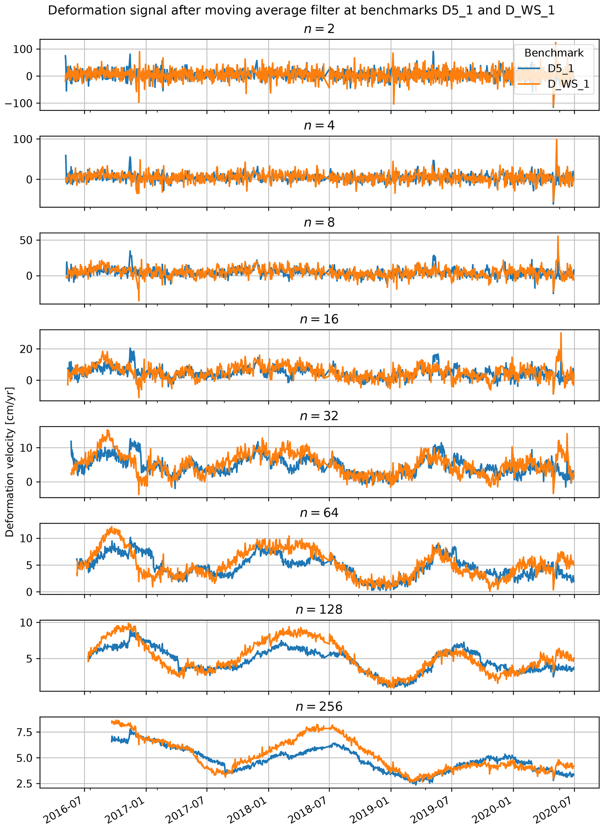
Figure B1Smoothed deformation signal, shown for an increasing length (in days) of the moving average filter. The filter only includes historic observations and is not “centred” to match the properties of an operational system. The increasing time lag is visible for the subsequent filter lengths by the right shifting of the velocity peaks. For initial observations, a filter length of half the final length of the filter was accepted.
C1 State-of-the-art
See Table C1.
Zhang et al. (2021)Deng et al. (2021)Krkač et al. (2020)Bossi and Marcato (2019)Liu et al. (2021)Xie et al. (2019)Huang et al. (2017)Krkač et al. (2017)Logar et al. (2017)Zhu et al. (2017)Cai et al. (2016)Liu et al. (2014)Chen and Zeng (2013)Corominas et al. (2005)Neaupane and Achet (2004)Miao et al. (2022)Li et al. (2021)Liu et al. (2020)Li et al. (2020)Wang et al. (2019)Yang et al. (2019)Li et al. (2018)Miao et al. (2018)Ma et al. (2017)Wen et al. (2017)Cao et al. (2016)Zhou et al. (2016)Jiang and Chen (2016)Lian et al. (2015)Ren et al. (2015)Du et al. (2013)Table C1Examples of different integration methods, linking hydro-meteorological conditions to deformation time series, and associated case studies. Most studies are at deep-seated landslides that did not undergo catastrophic collapse. Studies with and without reservoir level as observation are grouped together. Updated after van Natijne et al. (2020).
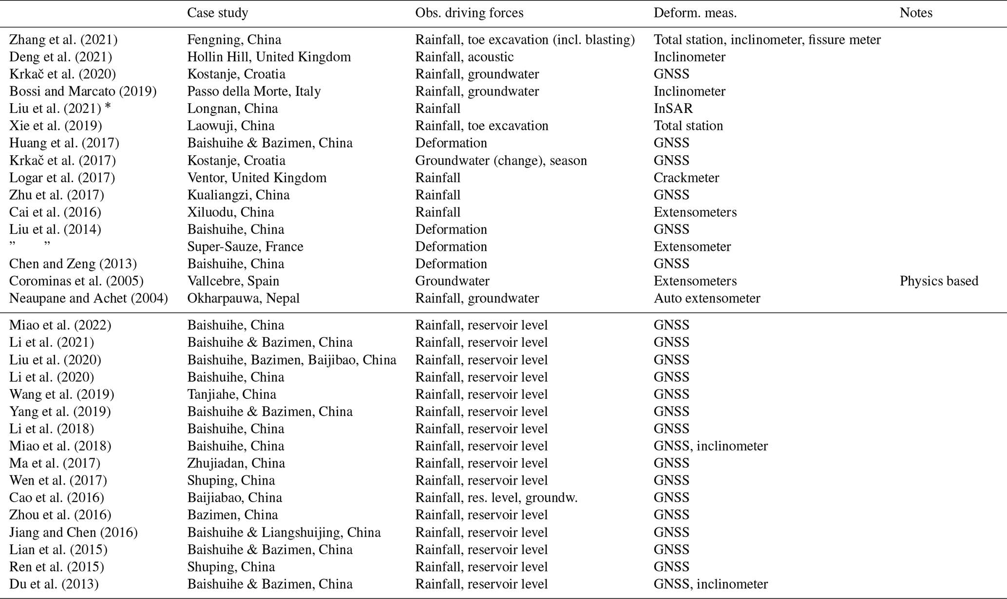
* Analysis, allows for prediction.
No specific algorithms or code has been developed for this study. The scripts used for the different runs consisted of a series of standard building blocks available within TensorFlow with their settings as mentioned in the text (https://doi.org/10.5281/zenodo.4724125, TensorFlow Developers, 2022).
The variables ERA5/tp, ERA5/swe, ERA5/smlt, ERA5/swvl4, and ERA5/t2m are freely available from the ECMWF ERA5 Land reanalysis (https://doi.org/10.24381/CDS.E2161BAC, Muñoz Sabater, 2019), hosted by Copernicus Climate Data Store. The variable GPM/precipitationCal is freely available from the Integrated Multi-satellitE Retrievals for GPM (IMERG) algorithm of the Global Precipitation Measurement (GPM) mission (https://doi.org/10.5067/GPM/IMERG/3B-HH-E/06, Huffman et al., 2019), hosted by NASA. The variable SMAP/sm_profile is freely available from SMAP L4 (https://doi.org/10.5067/08S1A6811J0U, Entekhabi et al., 2010; Reichle et al., 2022), hosted by the University of Colorado Boulder. The variable GLEAM/SMroot is freely available from the “Global Land Evaporation Amsterdam Model” (GLEAM) (https://www.gleam.eu/, Koppa and Rains, 2021; Martens et al., 2017; Miralles et al., 2011). The deformation time series (ATS/D_WS_1, ATS/D5_1) were provided by the Federal State of Tyrol (https://www.tirol.gv.at/sicherheit/geoinformation/vermessung-monitoring/monitoring/, Land Tirol, Department of Geoinformation, 2021).
ALvN: methodology, software, formal analysis, writing – original draft. TAB: conceptualization, writing – review & editing, supervision. TZ: resources, writing – review & editing. JP: resources, writing – review & editing. RCL: writing – review & editing, supervision.
The contact author has declared that none of the authors has any competing interests.
Publisher’s note: Copernicus Publications remains neutral with regard to jurisdictional claims in published maps and institutional affiliations.
This article is part of the special issue “Advances in machine learning for natural hazards risk assessment”. It is not associated with a conference.
This research has been supported by the OPERANDUM (OPEn-air laboRAtories for Nature baseD solUtions to Manage hydro-meteo risks) project, which is funded by European Union's Horizon 2020 Framework Programme for research and innovation under grant no. 776848.
This paper was edited by Sabine Loos and reviewed by Katy Burrows and one anonymous referee.
Belward, A. S. and Skøien, J. O.: Who Launched What, When and Why; Trends in Global Land-Cover Observation Capacity from Civilian Earth Observation Satellites, ISPRS J. Photogramm., 103, 115–128, https://doi.org/10.1016/j.isprsjprs.2014.03.009, 2015. a
Bengio, Y., Simard, P., and Frasconi, P.: Learning Long-Term Dependencies with Gradient Descent Is Difficult, IEEE T. Neural Networ., 5, 157–166, https://doi.org/10.1109/72.279181, 1994. a
Bogaard, T. A. and Greco, R.: Landslide Hydrology: From Hydrology to Pore Pressure, WIRES Water, 3, 439–459, https://doi.org/10.1002/wat2.1126, 2015. a, b
Bossi, G. and Marcato, G.: Planning Landslide Countermeasure Works through Long Term Monitoring and Grey Box Modelling, Geosciences, 9, 185, https://doi.org/10.3390/geosciences9040185, 2019. a
Cai, Z., Xu, W., Meng, Y., Shi, C., and Wang, R.: Prediction of Landslide Displacement Based on GA-LSSVM with Multiple Factors, B. Eng. Geol. Environ., 75, 637–646, https://doi.org/10.1007/s10064-015-0804-z, 2016. a
Cao, Y., Yin, K., Alexander, D. E., and Zhou, C.: Using an Extreme Learning Machine to Predict the Displacement of Step-like Landslides in Relation to Controlling Factors, Landslides, 13, 725–736, https://doi.org/10.1007/s10346-015-0596-z, 2016. a
Carlà, T., Intrieri, E., Di Traglia, F., Nolesini, T., Gigli, G., and Casagli, N.: Guidelines on the Use of Inverse Velocity Method as a Tool for Setting Alarm Thresholds and Forecasting Landslides and Structure Collapses, Landslides, 14, 517–534, https://doi.org/10.1007/s10346-016-0731-5, 2017. a
Cerqueira, V., Torgo, L., and Soares, C.: A case study comparing machine learning with statistical methods for time series forecasting: size matters, J. Intell. Inf. Syst., 59, 415–433, https://doi.org/10.1007/s10844-022-00713-9, 2022. a
Chen, H. and Zeng, Z.: Deformation Prediction of Landslide Based on Improved Back-Propagation Neural Network, Cogn. Comput., 5, 56–62, https://doi.org/10.1007/s12559-012-9148-1, 2013. a
Colesanti, C. and Wasowski, J.: Investigating Landslides with Space-Borne Synthetic Aperture Radar (SAR) Interferometry, Eng. Geol., 88, 173–199, https://doi.org/10.1016/j.enggeo.2006.09.013, 2006. a
Connor, J., Martin, R., and Atlas, L.: Recurrent Neural Networks and Robust Time Series Prediction, IEEE T. Neural Networ., 5, 240–254, https://doi.org/10.1109/72.279188, 1994. a
Corominas, J., Moya, J., Ledesma, A., Lloret, A., and Gili, J. A.: Prediction of Ground Displacements and Velocities from Groundwater Level Changes at the Vallcebre Landslide (Eastern Pyrenees, Spain), Landslides, 2, 83–96, https://doi.org/10.1007/s10346-005-0049-1, 2005. a
Crosetto, M., Solari, L., Mróz, M., Balasis-Levinsen, J., Casagli, N., Frei, M., Oyen, A., Moldestad, D. A., Bateson, L., Guerrieri, L., Comerci, V., and Andersen, H. S.: The Evolution of Wide-Area DInSAR: From Regional and National Services to the European Ground Motion Service, Remote Sens., 12, 2043, https://doi.org/10.3390/rs12122043, 2020. a
Deng, L., Smith, A., Dixon, N., and Yuan, H.: Machine Learning Prediction of Landslide Deformation Behaviour Using Acoustic Emission and Rainfall Measurements, Eng. Geol., 293, 106315, https://doi.org/10.1016/j.enggeo.2021.106315, 2021. a
Du, J., Yin, K., and Lacasse, S.: Displacement Prediction in Colluvial Landslides, Three Gorges Reservoir, China, Landslides, 10, 203–218, https://doi.org/10.1007/s10346-012-0326-8, 2013. a
Entekhabi, D., Njoku, E. G., O'Neill, P. E., Kellogg, K. H., Crow, W. T., Edelstein, W. N., Entin, J. K., Goodman, S. D., Jackson, T. J., Johnson, J., Kimball, J., Piepmeier, J. R., Koster, R. D., Martin, N., McDonald, K. C., Moghaddam, M., Moran, S., Reichle, R., Shi, J. C., Spencer, M. W., Thurman, S. W., Tsang, L., and Van Zyl, J.: The Soil Moisture Active Passive (SMAP) Mission, P. IEEE, 98, 704–716, https://doi.org/10.1109/JPROC.2010.2043918, 2010. a, b
Fell, R., Corominas, J., Bonnard, C., Cascini, L., Leroi, E., and Savage, W. Z.: Guidelines for Landslide Susceptibility, Hazard and Risk Zoning for Land-Use Planning, Eng. Geol., 102, 99–111, https://doi.org/10.1016/j.enggeo.2008.03.014, 2008. a, b
Gholamy, A., Kreinovich, V., and Kosheleva, O.: Why 70/30 or 80/20 Relation between Training and Testing Sets: A Pedagogical Explanation, Departmental Technical Reports (CS), https://scholarworks.utep.edu/cs_techrep/1209 (last access: 8 September 2022), 2018. a
Guzzetti, F., Carrara, A., Cardinali, M., and Reichenbach, P.: Landslide Hazard Evaluation: A Review of Current Techniques and Their Application in a Multi-Scale Study, Central Italy, Geomorphology, 31, 181–216, https://doi.org/10.1016/S0169-555X(99)00078-1, 1999. a, b
Guzzetti, F., Gariano, S. L., Peruccacci, S., Brunetti, M. T., Marchesini, I., Rossi, M., and Melillo, M.: Geographical Landslide Early Warning Systems, Earth-Sci. Rev., 200, 102973, https://doi.org/10.1016/j.earscirev.2019.102973, 2020. a
Hanssen, R. F.: Radar Interferometry: Data Interpretation and Error Analysis, Remote Sensing and Digital Image Processing, vol. 2, Springer Netherlands, Dordrecht, https://doi.org/10.1007/0-306-47633-9, 2001. a
Hartke, S. H., Wright, D. B., Kirschbaum, D. B., Stanley, T. A., and Li, Z.: Incorporation of Satellite Precipitation Uncertainty in a Landslide Hazard Nowcasting System, J. Hydrometeorol., 21, 1741–1759, https://doi.org/10.1175/JHM-D-19-0295.1, 2020. a
Heggen, R. J.: Normalized Antecedent Precipitation Index, J. Hydrol. Eng., 6, 377–381, https://doi.org/10.1061/(ASCE)1084-0699(2001)6:5(377), 2001. a
Herrera, G., Mateos, R. M., García-Davalillo, J. C., Grandjean, G., Poyiadji, E., Maftei, R., Filipciuc, T.-C., Jemec Auflič, M., Jež, J., Podolszki, L., Trigila, A., Iadanza, C., Raetzo, H., Kociu, A., Przyłucka, M., Kułak, M., Sheehy, M., Pellicer, X. M., McKeown, C., Ryan, G., Kopačková, V., Frei, M., Kuhn, D., Hermanns, R. L., Koulermou, N., Smith, C. A., Engdahl, M., Buxó, P., Gonzalez, M., Dashwood, C., Reeves, H., Cigna, F., Liščák, P., Pauditš, P., Mikulėnas, V., Demir, V., Raha, M., Quental, L., Sandić, C., Fusi, B., and Jensen, O. A.: Landslide Databases in the Geological Surveys of Europe, Landslides, 15, 359–379, https://doi.org/10.1007/s10346-017-0902-z, 2018. a
Hill, T., Marquez, L., O'Connor, M., and Remus, W.: Artificial Neural Network Models for Forecasting and Decision Making, Int. J. Forecasting, 10, 5–15, https://doi.org/10.1016/0169-2070(94)90045-0, 1994. a
Hilley, G. E., Bürgmann, R., Ferretti, A., Novali, F., and Rocca, F.: Dynamics of Slow-Moving Landslides from Permanent Scatterer Analysis, Science, 304, 1952–1955, https://doi.org/10.1126/science.1098821, 2004. a
Hochreiter, S.: The Vanishing Gradient Problem during Learning Recurrent Neural Nets and Problem Solutions, Int. J. Uncertain. Fuzz., 06, 107–116, https://doi.org/10.1142/S0218488598000094, 1998. a
Hochreiter, S. and Schmidhuber, J.: Long Short-Term Memory, Neural Comput., 9, 1735–1780, https://doi.org/10.1162/neco.1997.9.8.1735, 1997. a, b, c
Hornik, K., Stinchcombe, M., and White, H.: Multilayer Feedforward Networks Are Universal Approximators, Neural Networks, 2, 359–366, https://doi.org/10.1016/0893-6080(89)90020-8, 1989. a
Huang, F., Huang, J., Jiang, S., and Zhou, C.: Landslide Displacement Prediction Based on Multivariate Chaotic Model and Extreme Learning Machine, Eng. Geol., 218, 173–186, https://doi.org/10.1016/j.enggeo.2017.01.016, 2017. a
Huffman, G., Stocker, E., Bolvin, D., Nelkin, E., and Jackson, T.: GPM IMERG Early Precipitation L3 Half Hourly 0.1 Degree × 0.1 Degree V06, NASA [data set], https://doi.org/10.5067/GPM/IMERG/3B-HH-E/06, 2019. a, b
Intrieri, E., Raspini, F., Fumagalli, A., Lu, P., Del Conte, S., Farina, P., Allievi, J., Ferretti, A., and Casagli, N.: The Maoxian Landslide as Seen from Space: Detecting Precursors of Failure with Sentinel-1 Data, Landslides, 15, 123–133, https://doi.org/10.1007/s10346-017-0915-7, 2018. a
Jain, A., Jianchang Mao, and Mohiuddin, K.: Artificial Neural Networks: A Tutorial, Computer, 29, 31–44, https://doi.org/10.1109/2.485891, 1996. a
Jiang, P. and Chen, J.: Displacement Prediction of Landslide Based on Generalized Regression Neural Networks with K-Fold Cross-Validation, Neurocomputing, 198, 40–47, https://doi.org/10.1016/j.neucom.2015.08.118, 2016. a
Kingma, D. P. and Ba, J.: Adam: A Method for Stochastic Optimization, in: 3rd International Conference for Learning Representations, arXiv, https://doi.org/10.48550/arXiv.1412.6980, 22 December 2014. a
Kirschbaum, D. and Stanley, T.: Satellite-Based Assessment of Rainfall-Triggered Landslide Hazard for Situational Awareness, Earth's Future, 6, 505–523, https://doi.org/10.1002/2017EF000715, 2018. a
Kohler, M. A. and Linsley, R. K.: Predicting the Runoff from Storm Rainfall, vol. 30, US Department of Commerce, Weather Bureau, https://books.google.nl/books?id=XMtaTBhT5p4C&printsec=frontcover (last access: 17 August 2022), 1951. a
Koppa, A., and Rains, D.: Global Land Evaporation Amsterdam Model (GLEAM) v3.5 [data set], https://www.gleam.eu (last access: 13 April 2021), 2021. a
Krkač, M., Špoljarić, D., Bernat, S., and Arbanas, S. M.: Method for Prediction of Landslide Movements Based on Random Forests, Landslides, 14, 947–960, https://doi.org/10.1007/s10346-016-0761-z, 2017. a, b
Krkač, M., Bernat Gazibara, S., Arbanas, Z., Sečanj, M., and Mihalić Arbanas, S.: A Comparative Study of Random Forests and Multiple Linear Regression in the Prediction of Landslide Velocity, Landslides, 17, 2515–2531, https://doi.org/10.1007/s10346-020-01476-6, 2020. a, b, c, d
Land Tirol, Department of Geoinformation: Vögelsberg deformation time series, Land Tirol [data set], https://www.tirol.gv.at/sicherheit/geoinformation/vermessung-monitoring/monitoring/ (last access: 20 October 2023), 2021. a
Li, C., Criss, R. E., Fu, Z., Long, J., and Tan, Q.: Evolution Characteristics and Displacement Forecasting Model of Landslides with Stair-Step Sliding Surface along the Xiangxi River, Three Gorges Reservoir Region, China, Eng. Geol., 283, 105961, https://doi.org/10.1016/j.enggeo.2020.105961, 2021. a
Li, H., Xu, Q., He, Y., and Deng, J.: Prediction of Landslide Displacement with an Ensemble-Based Extreme Learning Machine and Copula Models, Landslides, 15, 2047–2059, https://doi.org/10.1007/s10346-018-1020-2, 2018. a
Li, H., Xu, Q., He, Y., Fan, X., and Li, S.: Modeling and Predicting Reservoir Landslide Displacement with Deep Belief Network and EWMA Control Charts: A Case Study in Three Gorges Reservoir, Landslides, 17, 693–707, https://doi.org/10.1007/s10346-019-01312-6, 2020. a
Lian, C., Zeng, Z., Yao, W., and Tang, H.: Multiple Neural Networks Switched Prediction for Landslide Displacement, Eng. Geol., 186, 91–99, https://doi.org/10.1016/j.enggeo.2014.11.014, 2015. a
Lins, H. F.: USGS Hydro-Climatic Data Network 2009 (HCDN-2009), Fact Sheet 2012-3047, USGS, 2012. a
Liu, Y., Qiu, H., Yang, D., Liu, Z., Ma, S., Pei, Y., Zhang, J., and Tang, B.: Deformation Responses of Landslides to Seasonal Rainfall Based on InSAR and Wavelet Analysis, Landslides, 19, 199–210, https://doi.org/10.1007/s10346-021-01785-4, 2021. a
Liu, Z., Shao, J., Xu, W., Chen, H., and Shi, C.: Comparison on Landslide Nonlinear Displacement Analysis and Prediction with Computational Intelligence Approaches, Landslides, 11, 889–896, https://doi.org/10.1007/s10346-013-0443-z, 2014. a
Liu, Z.-Q., Guo, D., Lacasse, S., Li, J.-h., Yang, B.-b., and Choi, J.-c.: Algorithms for Intelligent Prediction of Landslide Displacements, J. Zhejiang Univ. Sci. A, 21, 412–429, https://doi.org/10.1631/jzus.A2000005, 2020. a
Logar, J., Turk, G., Marsden, P., and Ambrožič, T.: Prediction of rainfall induced landslide movements by artificial neural networks, Nat. Hazards Earth Syst. Sci. Discuss. [preprint], https://doi.org/10.5194/nhess-2017-253, 2017. a
Ma, J., Tang, H., Liu, X., Hu, X., Sun, M., and Song, Y.: Establishment of a Deformation Forecasting Model for a Step-like Landslide Based on Decision Tree C5.0 and Two-Step Cluster Algorithms: A Case Study in the Three Gorges Reservoir Area, China, Landslides, 14, 1275–1281, https://doi.org/10.1007/s10346-017-0804-0, 2017. a
Makridakis, S., Spiliotis, E., and Assimakopoulos, V.: Statistical and Machine Learning Forecasting Methods: Concerns and Ways Forward, PLOS One, 13, e0194889, https://doi.org/10.1371/journal.pone.0194889, 2018. a
Mansour, M. F., Morgenstern, N. R., and Martin, C. D.: Expected Damage from Displacement of Slow-Moving Slides, Landslides, 8, 117–131, https://doi.org/10.1007/s10346-010-0227-7, 2011. a
Martens, B., Miralles, D. G., Lievens, H., van der Schalie, R., de Jeu, R. A. M., Fernández-Prieto, D., Beck, H. E., Dorigo, W. A., and Verhoest, N. E. C.: GLEAM v3: satellite-based land evaporation and root-zone soil moisture, Geosci. Model Dev., 10, 1903–1925, https://doi.org/10.5194/gmd-10-1903-2017, 2017. a, b
Miao, F., Wu, Y., Xie, Y., and Li, Y.: Prediction of Landslide Displacement with Step-like Behavior Based on Multialgorithm Optimization and a Support Vector Regression Model, Landslides, 15, 475–488, https://doi.org/10.1007/s10346-017-0883-y, 2018. a
Miao, F., Xie, X., Wu, Y., and Zhao, F.: Data Mining and Deep Learning for Predicting the Displacement of “Step-like” Landslides, Sensors, 22, 481, https://doi.org/10.3390/s22020481, 2022. a, b, c
Miralles, D. G., Holmes, T. R. H., De Jeu, R. A. M., Gash, J. H., Meesters, A. G. C. A., and Dolman, A. J.: Global land-surface evaporation estimated from satellite-based observations, Hydrol. Earth Syst. Sci., 15, 453–469, https://doi.org/10.5194/hess-15-453-2011, 2011. a, b
Muñoz Sabater, J.: ERA5-Land Hourly Data from 2001 to Present, Copernicus Climate Change Service (C3S) Climate Data Store (CDS) [data set], https://doi.org/10.24381/CDS.E2161BAC, 2019. a, b, c, d
Neaupane, K. and Achet, S.: Use of Backpropagation Neural Network for Landslide Monitoring: A Case Study in the Higher Himalaya, Eng. Geol., 74, 213–226, https://doi.org/10.1016/j.enggeo.2004.03.010, 2004. a
Nie, W., Krautblatter, M., Leith, K., Thuro, K., and Festl, J.: A modified tank model including snowmelt and infiltration time lags for deep-seated landslides in alpine environments (Aggenalm, Germany), Nat. Hazards Earth Syst. Sci., 17, 1595–1610, https://doi.org/10.5194/nhess-17-1595-2017, 2017. a
Novellino, A., Cesarano, M., Cappelletti, P., Di Martire, D., Di Napoli, M., Ramondini, M., Sowter, A., and Calcaterra, D.: Slow-Moving Landslide Risk Assessment Combining Machine Learning and InSAR Techniques, CATENA, 203, 105317, https://doi.org/10.1016/j.catena.2021.105317, 2021. a
Parajka, J., Kohnová, S., Merz, R., Szolgay, J., Hlavčová, K., and Blöschl, G.: Comparative Analysis of the Seasonality of Hydrological Characteristics in Slovakia and Austria, Hydrolog. Sci. J., 54, 456–473, https://doi.org/10.1623/hysj.54.3.456, 2009. a
Pfeiffer, J., Zieher, T., Schmieder, J., Rutzinger, M., and Strasser, U.: Spatio-temporal Assessment of the Hydrological Drivers of an Active Deep-seated Gravitational Slope Deformation: The Vögelsberg Landslide in Tyrol (Austria), Earth Surf. Proc. Land., 46, 1865–1881, https://doi.org/10.1002/esp.5129, 2021. a, b, c, d, e, f, g, h, i, j, k
Reichle, R., De Lannoy, G., Koster, R., Crow, W., Kimball, J., and Liu, Q.: SMAP L4 global 3-hourly 9 km EASE-grid surface and root zone soil moisture, version 6, NSIDC [data set], https://doi.org/10.5067/08S1A6811J0U, 2022. a, b
Ren, F., Wu, X., Zhang, K., and Niu, R.: Application of Wavelet Analysis and a Particle Swarm-Optimized Support Vector Machine to Predict the Displacement of the Shuping Landslide in the Three Gorges, China, Environ. Earth Sci., 73, 4791–4804, https://doi.org/10.1007/s12665-014-3764-x, 2015. a
Stanley, T. A., Kirschbaum, D. B., Benz, G., Emberson, R. A., Amatya, P. M., Medwedeff, W., and Clark, M. K.: Data-Driven Landslide Nowcasting at the Global Scale, Front. Earth Sci., 9, 640043, https://doi.org/10.3389/feart.2021.640043, 2021. a
TensorFlow Developers: TensorFlow, Zenodo [code], https://doi.org/10.5281/zenodo.4724125, 2022. a, b
Thomas, M. A., Collins, B. D., and Mirus, B. B.: Assessing the Feasibility of Satellite-based Thresholds for Hydrologically Driven Landsliding, Water Resour. Res., 55, 9006–9023, https://doi.org/10.1029/2019WR025577, 2019. a
van Asch, T. W. J., van Beek, L., and Bogaard, T.: Problems in Predicting the Mobility of Slow-Moving Landslides, Eng. Geol., 91, 46–55, https://doi.org/10.1016/j.enggeo.2006.12.012, 2007. a
van Natijne, A., Bogaard, T., van Leijen, F., Hanssen, R., and Lindenbergh, R.: World-Wide InSAR Sensitivity Index for Landslide Deformation Tracking, Int. J. Appl. Earth Obs., 111, 102829, https://doi.org/10.1016/j.jag.2022.102829, 2022. a
van Natijne, A. L., Lindenbergh, R. C., and Bogaard, T. A.: Machine Learning: New Potential for Local and Regional Deep-Seated Landslide Nowcasting, Sensors, 20, 1425, https://doi.org/10.3390/s20051425, 2020. a, b, c
Wang, Y., Tang, H., Wen, T., Ma, J., Zou, Z., and Xiong, C.: Point and Interval Predictions for Tanjiahe Landslide Displacement in the Three Gorges Reservoir Area, China, Geofluids, 2019, 8985325, https://doi.org/10.1155/2019/8985325, 2019. a
Wen, T., Tang, H., Wang, Y., Lin, C., and Xiong, C.: Landslide displacement prediction using the GA-LSSVM model and time series analysis: a case study of Three Gorges Reservoir, China, Nat. Hazards Earth Syst. Sci., 17, 2181–2198, https://doi.org/10.5194/nhess-17-2181-2017, 2017. a
World Meteorological Organization (WMO): WMO Atlas of Mortality and Economic Losses from Weather, Climate and Water Extremes (1970–2019) (WMO-no. 1267), Tech. Rep. 1267, WMO, Geneva, https://library.wmo.int/idurl/4/57564 (last access: 8 September 2022), 2021. a
Xie, P., Zhou, A., and Chai, B.: The Application of Long Short-Term Memory (LSTM) Method on Displacement Prediction of Multifactor-Induced Landslides, IEEE Access, 7, 54305–54311, https://doi.org/10.1109/ACCESS.2019.2912419, 2019. a
Yang, B., Yin, K., Lacasse, S., and Liu, Z.: Time Series Analysis and Long Short-Term Memory Neural Network to Predict Landslide Displacement, Landslides, 16, 677–694, https://doi.org/10.1007/s10346-018-01127-x, 2019. a, b
Yatheendradas, S., Kirschbaum, D., Nearing, G., Vrugt, J. A., Baum, R. L., Wooten, R., Lu, N., and Godt, J. W.: Bayesian Analysis of the Impact of Rainfall Data Product on Simulated Slope Failure for North Carolina Locations, Computat. Geosci., https://doi.org/10.1007/s10596-018-9804-y, 2019. a
Zhang, X., Zhu, C., He, M., Dong, M., Zhang, G., and Zhang, F.: Failure Mechanism and Long Short-Term Memory Neural Network Model for Landslide Risk Prediction, Remote Sens., 14, 166, https://doi.org/10.3390/rs14010166, 2021. a
Zhou, C., Yin, K., Cao, Y., and Ahmed, B.: Application of Time Series Analysis and PSO–SVM Model in Predicting the Bazimen Landslide in the Three Gorges Reservoir, China, Eng. Geol., 204, 108–120, https://doi.org/10.1016/j.enggeo.2016.02.009, 2016. a
Zhu, X., Xu, Q., Tang, M., Nie, W., Ma, S., and Xu, Z.: Comparison of Two Optimized Machine Learning Models for Predicting Displacement of Rainfall-Induced Landslide: A Case Study in Sichuan Province, China, Eng. Geol., 218, 213–222, https://doi.org/10.1016/j.enggeo.2017.01.022, 2017. a
Zhu, Z., Wulder, M. A., Roy, D. P., Woodcock, C. E., Hansen, M. C., Radeloff, V. C., Healey, S. P., Schaaf, C., Hostert, P., Strobl, P., Pekel, J.-F., Lymburner, L., Pahlevan, N., and Scambos, T. A.: Benefits of the Free and Open Landsat Data Policy, Remote SENS. Environ., 224, 382–385, https://doi.org/10.1016/j.rse.2019.02.016, 2019. a
Zieher, T., Pfeiffer, J., van Natijne, A., and Lindenbergh, R.: Integrated Monitoring of a Slowly Moving Landslide Based on Total Station Measurements, Multi-Temporal Terrestrial Laser Scanning and Space-Borne Interferometric Synthetic Aperture Radar, in: 2021 IEEE International Geoscience and Remote Sensing Symposium IGARSS, IEEE, Brussels, Belgium, 11–16 July 2021, 942–945, https://doi.org/10.1109/IGARSS47720.2021.9553324, 2021. a
- Abstract
- Introduction
- Data-driven modelling approaches
- Case study: the Vögelsberg landslide
- Methodology
- Results
- Discussion
- Conclusions
- Appendix A: Data
- Appendix B: Total Station
- Appendix C: Models
- Code availability
- Data availability
- Author contributions
- Competing interests
- Disclaimer
- Special issue statement
- Financial support
- Review statement
- References