the Creative Commons Attribution 4.0 License.
the Creative Commons Attribution 4.0 License.
 | 08 Sep 2023
The concept of event-size-dependent exhaustion and its application to paraglacial rockslides
Stefan Hergarten
Rockslides are a major hazard in mountainous regions. In formerly glaciated regions, the disposition mainly arises from oversteepened topography and decreases through time. However, little is known about this decrease and thus about the present-day hazard of huge, potentially catastrophic rockslides. This paper presents a new theoretical concept that combines the decrease in disposition with the power-law distribution of rockslide volumes found in several studies. The concept starts from a given initial set of potential events, which are randomly triggered through time at a probability that depends on event size. The developed theoretical framework is applied to paraglacial rockslides in the European Alps, where available data allow for constraining the parameters reasonably well. The results suggest that the probability of triggering increases roughly with the cube root of the volume. For small rockslides up to 1000 m3, an exponential decrease in the frequency with an e-folding time longer than 65 000 years is predicted. In turn, the predicted e-folding time is shorter than 2000 years for volumes of 10 km3, so the occurrence of such huge rockslides is unlikely at the present time. For the largest rockslide possible at the present time, a median volume of 0.5 to 1 km3 is predicted. With a volume of 0.27 km3, the artificially triggered rockslide that hit the Vaiont reservoir in 1963 is thus not extraordinarily large. Concerning its frequency of occurrence, however, it can be considered a 700- to 1200-year event.
- Article
(7658 KB) - Full-text XML
- BibTeX
- EndNote


Rockslides are a ubiquitous hazard in mountainous regions. The biggest rockslide in the European Alps since 1900 took place in 1963 at the Vaiont reservoir. It involved a volume of about 0.27 km3. Owing to an overtopping of the dam, it claimed more than 2000 lives. However, the reservoir played an important part in triggering this huge rockslide, so it cannot be considered a natural event. The largest natural rockslides in the Alps since 1900 are considerably smaller (e.g., Gruner, 2006).
In turn, two huge rockslides with volumes of several cubic kilometers have been identified and dated. These are the Flims rockslide with a deposited volume of about 10 km3 (Aaron et al., 2020) in the carbonatic rocks of the Rhine Valley and the Köfels rockslide with a deposited volume of about 4 km3 (Zangerl et al., 2021) in the crystalline rocks of the Oetz valley. Estimates of the ages of these two giant events scatter by some 100 years (Deplazes et al., 2007; Nicolussi et al., 2015, and references therein). Within this scatter, however, both ages are about 9500 BP. These ages refute the older idea of triggering by glacial debuttressing. Since the inner Alpine valleys were largely free of ice by about 18 000 BP (e.g., Ivy-Ochs et al., 2008), an immediate relation to the deglaciation of the respective valleys can be excluded. Consequently, von Poschinger et al. (2006) concluded that rockslides of several cubic kilometers have to be taken into consideration also at present.
Although an immediate effect of deglaciation can be excluded for the Flims and Köfels rockslides, the former glaciation of the valleys plays a central part in rockslide disposition. In the context of paraglacial rock-slope failure, Cruden and Hu (1993) proposed the concept of exhaustion (see also Ballantyne, 2002a, b). The concept is similar to radioactive decay. Starting from an initial population of potentially unstable sites, it is assumed that each of them is triggered at a given probability per time λ. Then both the remaining number of potentially unstable sites and the rockslide frequency decrease like e−λt. Analyzing a small data set of 67 rockslides with volumes V≥ 1000 m3 (10−6 km3) from the Canadian Rocky Mountains, where 14 similar potentially unstable sites were found, Cruden and Hu (1993) estimated λ = 0.18 kyr−1, equivalent to an e-folding time = 5700 yr.
As a main limitation, however, the estimate T = 5700 yr refers to the total number of rockslides with V≥ 1000 m3. Whether this estimate could be transferred to rockslides of any given size is nontrivial. If this result could be transferred to rockslides of any size in the Alps, the present-day probability even of huge rockslides would be only by a factor of lower than it was at the time of the Flims and Köfels rockslides.
Analyzing the statistical distribution of landslide sizes became popular a few years after the concept of exhaustion was proposed, presumably pushed forward by the comprehensive analysis of several thousand landslides in Taiwan by Hovius et al. (1997). Reanalyzing several data sets, Malamud et al. (2004) found that landslides in unconsolidated material as well as rockfalls and rockslides follow a power-law distribution over some range in size. The exponent of the power law was found to be independent of the triggering mechanism (e.g., earthquakes, rainstorms, or rapid snowmelt) but is considerably lower for rockfalls and rockslides than for landslides in unconsolidated material. The distinct dependence on the material was confirmed by Brunetti et al. (2009). For deeper insights into the scaling properties of landslides, the review article of Tebbens (2020) is recommended.
Several models addressing the power-law distribution of landslides have been developed so far (Densmore et al., 1998; Hergarten and Neugebauer, 1998; Hergarten, 2012; Alvioli et al., 2014; Liucci et al., 2017; Jeandet et al., 2019; Campforts et al., 2020). Some of these studies discussed landslides in the context of self-organized criticality (SOC). The idea of SOC was introduced by Bak et al. (1987) and promised to become a unifying theoretical concept for dynamic systems that generate events of various sizes following a power-law distribution. Jensen (1998) characterized SOC systems as slowly driven, interaction-dominated threshold systems. In the context of landslides, relief is generated directly or indirectly (e.g., in combination with fluvial incision) by tectonics. This process is rather continuous and slow. In turn, landslides take place as discrete events if a threshold is exceeded and relief is diminished. A system that exhibits SOC approaches some kind of long-term equilibrium between long-term driving and instantaneous relaxation with power-law-distributed event sizes.
Now the question arises of how the idea of paraglacial exhaustion can be reconciled with the power-law distribution of rockslide sizes, perhaps in combination with SOC. While size distributions of rockfalls and rockslides were addressed in several studies during the previous decade (e.g., Bennett et al., 2012; Lari et al., 2014; Valagussa et al., 2014; Strunden et al., 2015; Tanyas et al., 2018; Hartmeyer et al., 2020; Mohadjer et al., 2020), only the two latest studies refer directly to paraglacial exhaustion. Mohadjer et al. (2020) attempted to estimate the total volume of rockfalls in a deglaciated valley at different timescales up to 11 000 years. In turn, Hartmeyer et al. (2020) investigated the rockfall activity at walls above a retreating glacier at much smaller spatial and temporal scales.
In this paper, a theoretical framework for event-size-dependent exhaustion is developed, which means that the decay constant λ depends on the event size. In the following section, it is illustrated that the Drossel–Schwabl forest-fire model, as one of the simplest models in the field of SOC, and the model for rockslide disposition proposed by Hergarten (2012) already predict such a behavior. In Sect. 3, the theoretical framework will be developed. This framework will be applied to the Alps in Sect. 4, and it will be investigated to what extent the sparse available data on large rockslides can be used to constrain the parameters.
2.1 The Drossel–Schwabl forest-fire model
Let us start with the Drossel–Schwabl forest-fire model (DS-FFM in the following) as an example. While several similar models in its spirit were developed soon after the idea of SOC became popular, the version proposed by Drossel and Schwabl (1992) with a simplification introduced by Grassberger (1993) attracted the greatest interest. Although obviously oversimplified, it was found later that it reproduces some properties of real wildfires quite well (Malamud et al., 1998; Zinck and Grimm, 2008; Krenn and Hergarten, 2009).
The DS-FFM is a stochastic cellular automaton model that is usually considered on a two-dimensional square lattice with periodic boundary conditions. Each site can be either empty or occupied by a tree. In each time step, a given number θ of new trees is planted at randomly selected sites, assuming that planting a tree at an already occupied site has no effect. Then a randomly selected site is ignited. If this site is occupied by a tree, this tree and the entire cluster of connected trees are burned. By default, only nearest-neighbor connections are considered.
Regardless of the initial condition, the DS-FFM self-organizes towards a quasi-steady state in which as many trees are burned as are planted on average. If the growth rate θ and the size of the model are sufficiently large, about 40 % of all sites are occupied on average and the distribution of the fire sizes roughly follows a power law. The DS-FFM was investigated numerically and theoretically in numerous studies (e.g., Christensen et al., 1993; Henley, 1993; Clar et al., 1994; Pastor-Satorras and Vespignani, 2000; Pruessner and Jensen, 2002; Schenk et al., 2002; Hergarten and Krenn, 2011), resulting in a more or less complete understanding of its properties.
Let us now assume that the growth of new trees ceases suddenly at some time in the quasi-steady state so that the available clusters of trees are burned successively. Figure 1 shows an example computed on a small grid of 256 × 256 sites with θ=100. It is immediately recognized that the largest fires take place quite early. This property is owing to the mechanism of ignition. Each cluster of trees can be burned equivalently by igniting any of its trees. So the probability that a cluster of trees is burned is proportional to the cluster size (number of trees). This implies that large clusters are preferred to small clusters at any time. This property was already used by Hergarten and Krenn (2011) for deriving a semi-phenomenological explanation of the power-law distribution in the quasi-steady state and by Krenn and Hergarten (2009) for modifying the DS-FFM towards human-induced fires.
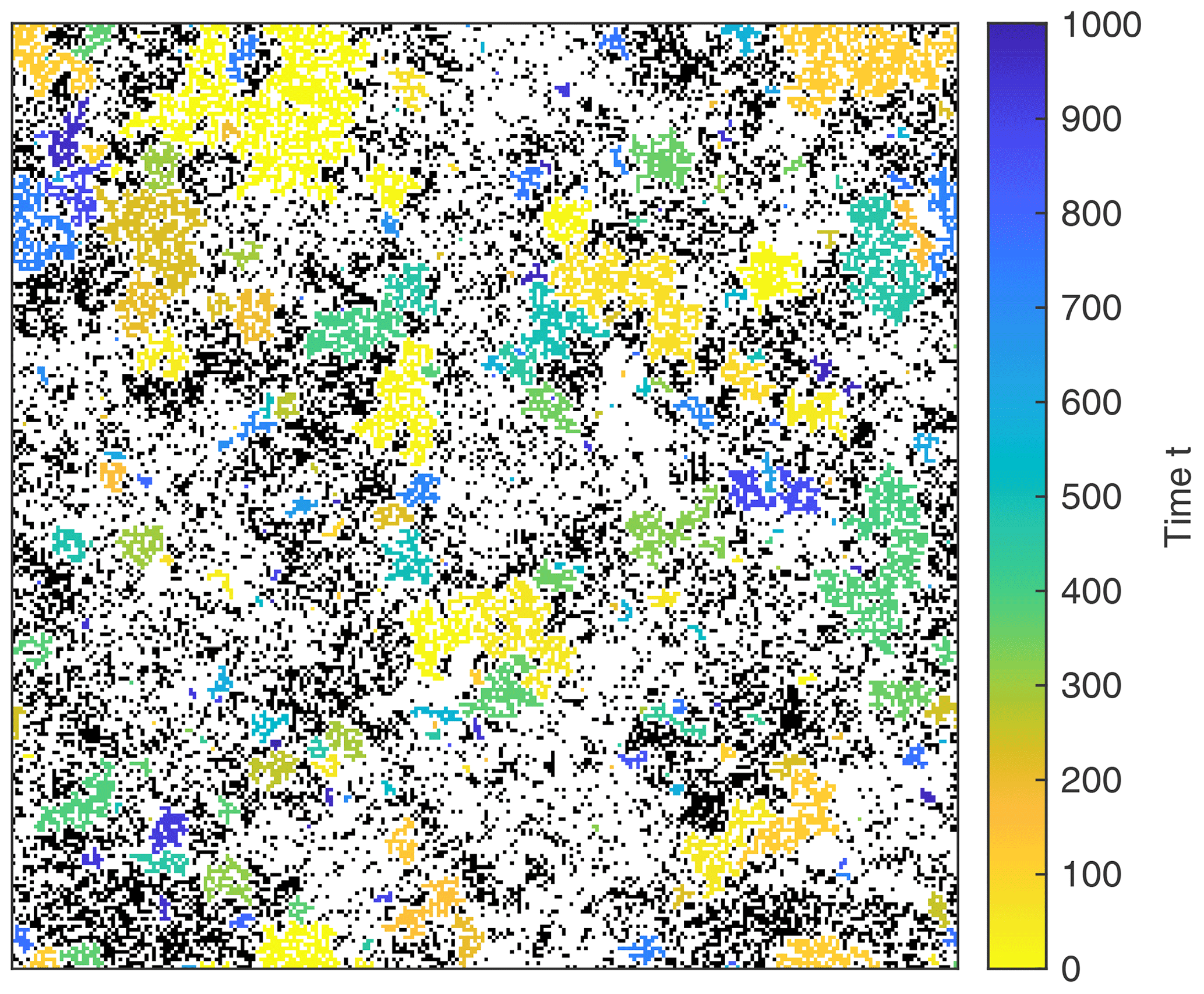
Figure 1Burned clusters of trees without regrowth on a 256 × 256 grid. One unit of time corresponds to one event of ignition. Colored patches correspond to clusters burned at different times. White sites were already empty in the beginning, while black clusters are still present after the simulated 1000 events of ignition.
Owing to the preference of large fires, the DS-FFM in a phase without regrowth is an example of event-size-dependent exhaustion. Figure 2 shows the size distribution of the fires derived from a simulation on a larger grid of 65 536 × 65 536 sites with θ = 10 000. It is immediately recognized that the distribution derived from the quasi-steady state (black curve) follows a power law only over a limited range. The rapid decline for s>105 is due to the finite growth rate θ. As explained by Hergarten and Krenn (2011), the excess of fires at the transition to the rapid decline (s≈105) is owing to the shape of large clusters and is thus a specific property of the DS-FFM, which is not relevant for the following considerations.
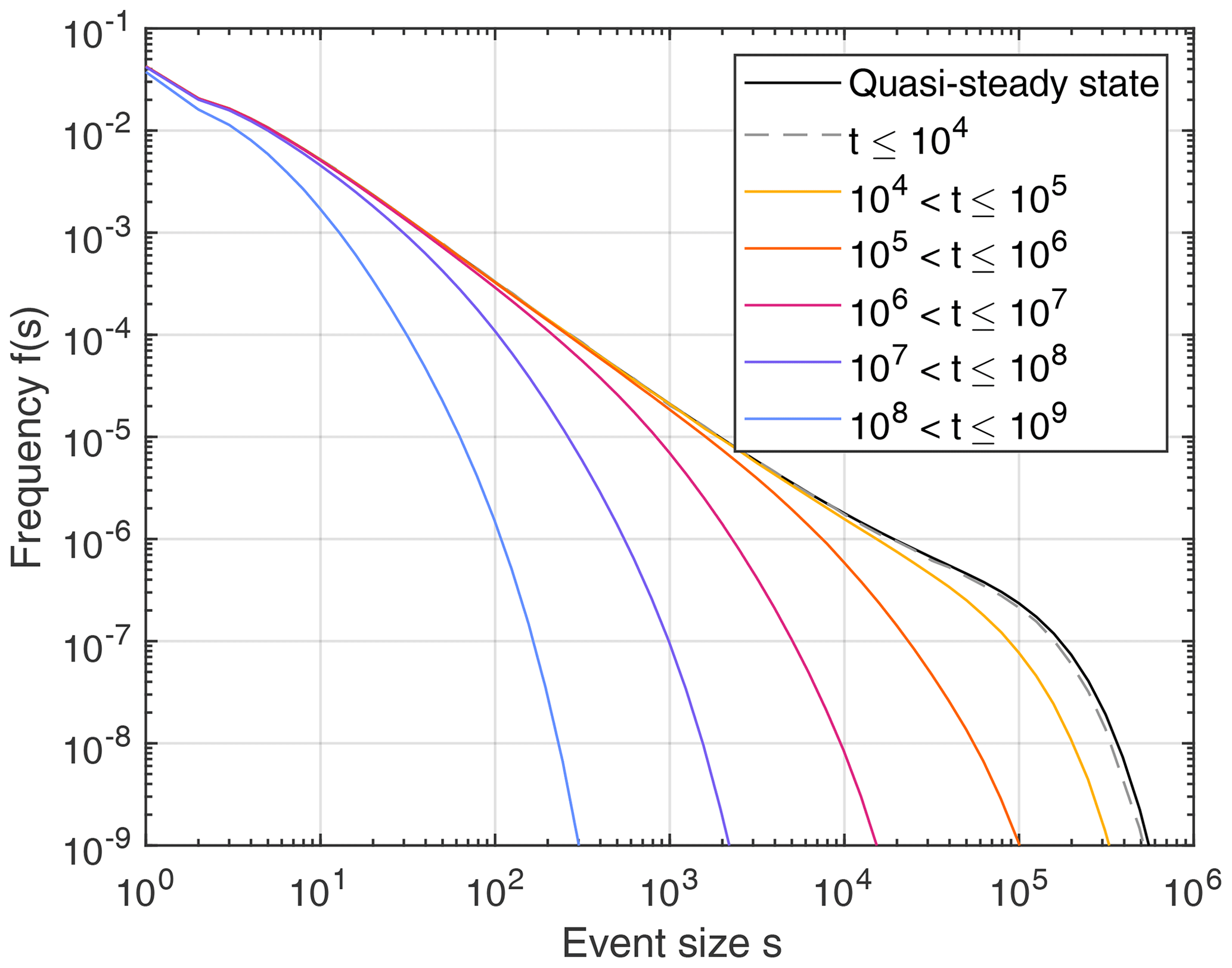
Figure 2Frequency of the fires in the DS-FFM during phases without growing trees. All distributions were obtained from simulations on a 65 536 × 65 536 grid with θ = 10 000 and smoothed by logarithmic binning with 10 bins per decade. The black curve describes the frequency of fires per ignition event in the quasi-steady state, while the other curves describe different time slices. These data were obtained by stacking 75 simulated sequences starting from different points of the quasi-steady state.
The distribution of the fires that take place during the first 10 000 steps after growth has ceased is almost identical to the distribution in the quasi-steady state. A small deficit is only visible at the tail. So the overall consumption of clusters during the first 10 000 steps is negligible, except for the largest clusters. The trend that large clusters are consumed more rapidly than small clusters is consolidated over larger time spans. In the time interval from t=105 to 106, the frequency of fires with sizes s≈105 is by more than 2 decades lower than in the quasi-steady state, while the frequency of fires with s⪅103 is still almost unaffected.
As a central result, the power-law distribution of the fires is consumed through time from the tail. In particular, the exponent (slope in the double-logarithmic plot) stays the same in principle, while only the range of the power law becomes shorter. Finally, however, the decay also affects the frequency of the smallest fires.
2.2 A simple model for rockslide disposition
Hergarten (2012) proposed a simple model for rockslide disposition. This model is based on topography alone and assumes that each site of a regular lattice may become unstable if exposed to a random trigger. The probability of failure p is assumed to be a function of the local slope S, measured in the direction of steepest descent among the eight nearest and diagonal neighbors. Sites with a slope below a given slope Smin always remain stable (p=0), while sites steeper than a given slope Smax become unstable whenever exposed to a trigger (p=1). A linear increase in probability,
is assumed in the range between Smin and Smax. As soon as a site becomes unstable, as much material as needed for reducing the slope to Smin is removed, and a trigger is applied to all eight neighbors. Depending on the topography, this may lead to large avalanches.
Applied to the topography of the Alps, the Himalayas, and the southern Rocky Mountains, the model reproduced the observed power-law distribution of rockslide volumes reasonably well. Differences between the considered mountain ranges were found concerning the transition from a power law to an exponential distribution at large volumes. However, the model has not been applied widely since then, except for the study on landslide dams by Argentin et al. (2021).
Figure 3 illustrates the application of the model to a region in Switzerland. Since the model has not been tested systematically for terrain models with less than 10 m grid spacing, the 2 m terrain model of Switzerland (Bundesamt für Landestopografie swisstopo, 2022) was resampled to 10 m grid spacing. Since the model is used only for illustration here, the parameter values and were adopted from Hergarten (2012) and Argentin et al. (2021). A total of 10 triggers per square kilometer were applied to the actual topography (so not a sequence of consecutive events).
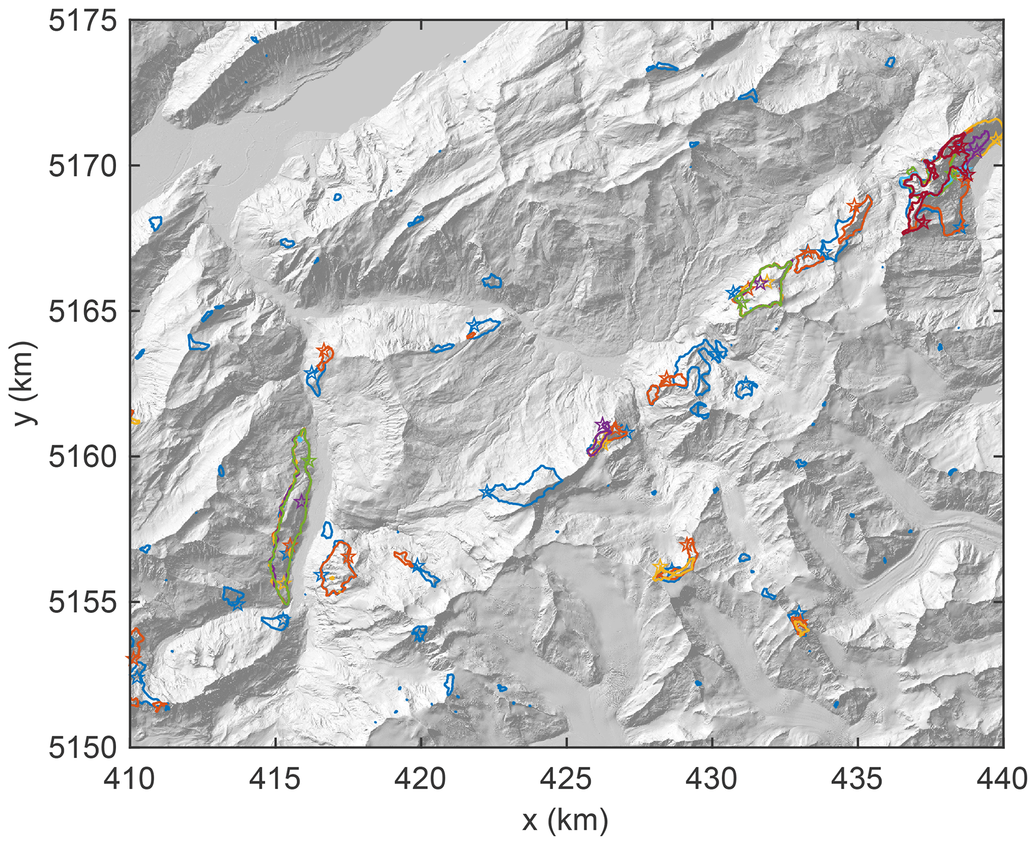
Figure 3Simulated rockslide sites for a part of Switzerland. In addition to the outlines of the unstable areas, the respective triggering points are also shown for events with V≥ 10−4 km3 (105 m3). Colors are just used for distinguishing overlapping outlines. Coordinates refer to UTM 32.
As the main point to be illustrated, different triggering points result in very similar events at some locations. At some other locations, events arising from different triggers are overlapping but differ in size. Both effects become stronger with increasing event size. This means that larger potential rockslides are more likely to be triggered than smaller potential rockslides in the model.
Qualitatively, this behavior is similar to that of the DS-FFM but more complex. Since randomness is not limited to triggering but is also part of the propagation of instability, even rockslides of different sizes may be triggered from the same point. In contrast to the DS-FFM, finding a quantitative relation between event size and probability of being triggered is not trivial for the rockslide model.
It is, however, recognized that the triggering points are not distributed uniformly in the area but are concentrated around the lower part of the outline. In this model, the initial instability preferably occurs at very steep sites and then predominantly propagates uphill since the uphill sites become steeper due to the removal of material. Accordingly, the increase in triggering probability with area (and thus also with volume) should be weaker than linear.
Let us assume that the process of exhaustion starts at t=0 from a given set of objects (potential events) described by a nondimensional size s. This size is defined in such a way that the probability λ of decay (generating an event) per time is proportional to s (as in the DS-FFM),
with a given value μ. Let ϕ(s,t) be the frequency density of the objects still there at time t. Since ϕ(s,t) refers to the number of objects of size s, it decreases according to
This leads to
where ϕ(s,0) is the initial frequency density of the objects.
Let us further assume that the objects initially follow a power-law (Pareto) distribution, which is most conveniently written in the cumulative form
with an exponent α. The cumulative frequency Φ(s,t) describes the expected number of objects with sizes greater than or equal to s at time t. In the context of statistics, Φ(s,t) is the complementary cumulative frequency, while the cumulative frequency originally refers to the number of objects smaller than s. For a power-law distribution, considering the complementary frequency simplifies the equations and allows for a convenient graphical representation as a straight line in a double-logarithmic diagram.
Since , the initial number of objects with sizes s≥1 is n. The respective frequency density is
which yields
in combination with Eq. (4).
Computing the cumulative frequency Φ(s,t) requires the integration of Eq. (7):
Substituting u=μσt, the integral can be transformed into
with the upper incomplete gamma function
The negative rate of change in ϕ(s,t) defines the frequency density of the events per unit time and at time t:
The respective cumulative frequency of the events per unit time, F(s,t), can be computed by performing the same steps as in Eqs. (8) and (9):
As an example, Fig. 4 shows the respective distributions for α=1.2 (similar to the DS-FFM) and μ=1 (which only affects the timescale). The two frequency densities f(s,t) and ϕ(s,t) are still close to the respective initial densities at over a considerable range of sizes. Their exponents differ by 1 (α vs. α+1). According to Eqs. (4) and (11), the actual frequency density drops below the respective power law by a factor of e at a size
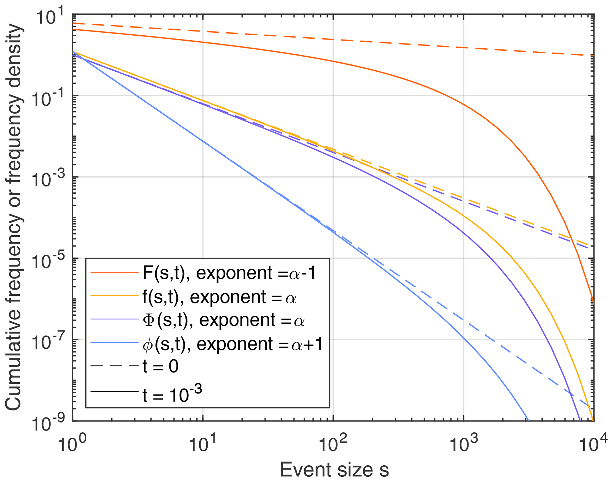
Figure 4Cumulative frequency and frequency density of the events per unit time (F(s,t), f(s,t)) and the objects still present (Φ(s,t), ϕ(s,t)) at t=0 and for α=1.2 and μ=1. All distributions were normalized to the total number n of objects with sizes s≥1 (n=1 in all equations).
Owing to this property, sc can be used for characterizing the transition from a power law to an exponential decrease at large event sizes. In this example, sc = 1000 at .
For the cumulative frequencies, the deviations from the respective power law extend towards smaller sizes compared to the frequency densities. The stronger deviation arises from the dependence of the cumulative frequency at size s on the frequency density of all greater sizes.
Applying the framework developed in Sect. 3 to paraglacial rockslides in a given region requires the definition of the event size s in the sense of Eq. (2) at first. This means that the probability of failure at a potential rockslide site is proportional to s. As discussed in Sect. 2.2, defining s is not straightforward here. So let us assume a general power-law relation
with a given exponent γ and a reference volume V0. Since μ in Eq. (2) is the decay constant λ for s=1, it is the decay constant for rockslides with a volume V=V0 here, and n (Eq. 5) is the initial number of potential rockslide sites with V≥V0.
If the shape of the detached body was independent of its volume, areas would be proportional to V⅔ and lengths proportional to V⅓. So assuming that failure can be initiated at each point of the fracture surface at the same probability would lead to . Taking into account that large detached bodies are relatively thinner than small bodies (Larsen et al., 2010) would result in but still considerably below 1. The simple model considered in Sect. 2.2 suggests that the length of the outcrop line might be the relevant property rather than the area, which would result in .
Keeping the exponent γ as an unknown parameter, forward modeling based on the concept of size-dependent exhaustion involves the four parameters γ, μ, α, and n. When referring to real-world data, however, it is not known when the process of exhaustion started. Therefore, a real-world time t0 must be assigned to the starting point t=0 used in the theoretical framework, which introduces an additional parameter.
Since data on the frequency of rockslides are sparse and the completeness of inventories is often an issue, validating the exhaustion model and constraining its parameters is challenging. For the European Alps as a whole, a combination of historical and prehistorical data is used in the following.
-
A total of 18 rockslides with volumes between 0.001 and 0.01 km3 (1 to 10 ×106 m3) took place from 1850 to 2020 CE. These are 15 events up to 2000 CE reported by Gruner (2006) and 3 events in the 21th century (Dents du Midi, 2006; Bondo 2011 and 2017).
-
Seven rockslides with volumes between 0.01 and 0.1 km3 (10 to 100 ×106 m3) took place from 1850 to 2020 CE (Gruner, 2006).
-
Two rockslides with volumes greater than 0.1 km3 took place from 1000 to 2020 CE (Gruner, 2006).
-
At t = 9450 BP, the largest potential rockslide volume is 10 km3, corresponding to the age (Deplazes et al., 2007) and volume (Aaron et al., 2020) of the Flims rockslide.
-
At t = 9500 BP, the second-largest potential rockslide volume is 4 km3, corresponding to the age (Nicolussi et al., 2015) and volume (Zangerl et al., 2021) of the Köfels rockslide.
-
At t = 3210 BP, the largest potential rockslide volume is 1.1 km3, corresponding to the Kandersteg rockslide (Singeisen et al., 2020).
-
At t = 4150 BP, the second-largest potential rockslide volume is 1 km3, corresponding to the Fernpass rockslide (Gruner, 2006).
Anthropogenically triggered rockslides were not taken into account in these data.
Constraints 4–7 differ from constraints 1–3 since they are not inventories over a given time span but refer to the largest or second-largest available volumes at a given time. The respective statistical distributions are described by rank-ordering statistics (e.g., Sornette, 2000, Chapter 6). Despite the different types of the data, they can be combined in a maximum likelihood formalism. The likelihood of a given parameter combination (γ, μ, α, n, and t0) is the product of seven factors then. The first three factors are the probabilities that 18, 5, and 2 events occur in the volume ranges and time spans defined in constraints 1–3. The fourth factor is the probability density of the volume of the largest potential rockslide at V = 10 km3 and t = 9450 BP. The remaining factors are obtained from the same principle. The respective expressions for the seven factors are developed in Appendix A.
However, the seven constraints defined above provide a very limited basis for constraining the five parameters γ, μ, α, n, and t0. Since these constraints refer to volumes V≥ 10−3 km3 (1 ×10⁶ m3), it would be useful to include information about smaller events from local inventories. As exhaustion predominantly affects the frequency of large events, it makes sense to assume that the power-law distribution typically found in local inventories defines the initial distribution, so the initial frequency density f(s,0) of the events follows a power law with the exponent α (Eq. 11). As reviewed by Brunetti et al. (2009), this exponent is typically in the range , where the subscript V indicates that this value refers to volume instead of the generic measure of event size s. The relation between αV and α is easily obtained from the cumulative frequency of the events at t=0,
with
While αV is used instead of α in the following, knowledge about αV from real-world inventories is not directly included in the maximum likelihood approach. The typical range is only used for checking whether the estimate obtained from the maximum likelihood approach is consistent with local inventories.
Technically, all computations were performed in terms of s (Eq. 14) instead of V and consequently using α instead of αV. The transfer to V and αV, which are more useful than s and α in the interpretation, was performed afterwards.
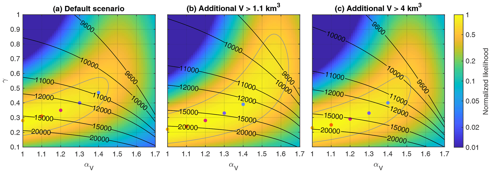
Figure 5Likelihood as a function of αV and γ for different scenarios. The maximum likelihood values taken over all combinations of the remaining parameters μ, n, and t0 are shown. Likelihood values are normalized to the maximum value, and the gray contour line refers to of the maximum likelihood. Black contour lines describe the obtained time t0 (BP) at which the process of exhaustion started. Colored dots refer to the points with the highest likelihood for αV=1, 1.1, 1.2, 1.3, and 1.4.
Figure 5a shows the likelihood as a function of the exponents αV and γ. For each combination of these two parameters, the respective values of μ, n, and t0 that maximize the likelihood were computed. Since absolute values of the likelihood have no immediate meaning, all values are normalized to the maximum values. In addition to the likelihood values, the obtained values of t0 are illustrated in the form of contour lines, while the obtained values of μ and n are not shown.
The highest likelihood is even achieved for αV=1 in combination with γ=0.28. However, the likelihood decreases only by a factor of 0.68 for αV=1.4 and γ=0.47. For a Gaussian likelihood function, the standard deviation would correspond to a reduction by a factor of , which is marked by the gray contour line. So the entire parameter region inside the gray line cannot be considered unlikely.
Qualitatively, however, the observed increase in likelihood towards smaller exponents αV makes sense. Since size-dependent exhaustion particularly reduces the frequency of large events, it may introduce a bias towards larger estimates of αV in rockslide inventories compared to the initial distribution. As illustrated in Fig. 4, the deviation from the power law increases continuously with increasing event size, so there is no distinct range of validity for the power-law distributions. As a consequence, any method that does not take into account the deviation from the power law explicitly will likely overestimate the exponent. So the real value of αV may be rather at the lower edge of the observed interval or even be slightly below 1.1.
The data set used for calibration is not only quite small but also potentially incomplete. For the inventories used for constraints 1 and 2, incompleteness should not be a serious problem. The inventory used for the third constraint is small and thus does not contribute much information, so an additional event would not change much. In turn, the assumptions on the largest or second-largest potential rockslide at a given time are more critical. As an example, the Kandersteg rockslide was assumed to be much older (t = 9600 BP; Tinner et al., 2005) than the recent estimate (t = 3210 BP; Singeisen et al., 2020) for several years. So constraints 6 and 7 would have been different a few years ago.
In general, constraints 4–7 based on rank ordering may be affected by the discovery of unknown huge rockslides, as well as by new estimates of ages or volumes of rockslides that are already known. Perhaps even more important, rockslides larger than those in constraints 4–7 may take place in the future.
To illustrate the effect of a potential incompleteness, it is assumed that the Kandersteg rockslide is not the largest potential event at t = 3210 BP but that there is one additional larger event. For the formalism, it makes no difference whether this event already took place or will take place in the future. As a moderate scenario, it is assumed that this additional event is smaller than the Köfels rockslide (). This scenario shifts the rank of the events in constraints 6 and 7 by one (Kandersteg to second and Fernpass to third).
As shown in Fig. 5b, this scenario shifts the likely range towards lower values of the exponent γ. According to its definition (Eq. 14), lower values of γ correspond to a weaker dependence of the decay constant on volume. So the exhaustion of large events becomes relatively slower then, which is the expected behavior if we assume an additional large event at a later time.
The third scenario (Fig. 5c) goes a step further by assuming that there was a potential event even larger than the Köfels rockslide but smaller than the Flims rockslide (4 km3 < V < 10 km3) at the time of the Kandersteg rockslide. This means that the rank of the Köfels rockslide in constraint 5 changes from second to third. However, the likelihood values shown in Fig. 5c reveal no further shift towards lower values of γ but even a small tendency back towards the default scenario (Fig. 5a).
In the following, the rockslide size distributions corresponding to the five dots in all three scenarios (Fig. 5a–c) are considered. This means that the values αV=1, 1.1, 1.2, 1.3, and 1.4 are considered for each scenario, while only the most likely values of the other parameters γ, μ, n, and t0 are used.
Let us now come back to the question about the size of the largest rockslide to be expected in the future in the Alps, i.e., for the largest potential rockslide volume at present (2020 CE). Let Φ(V,t) be the cumulative frequency at the present time (Eq. 9 expressed in terms of V instead of s). Then Φ(V0,t) is the total number of potential rockslides with V≥V0. Each of them is smaller than V at a probability . Raising this probability to the power of Φ(V0,t) yields the probability that all potential rockslides are smaller than V. Then
is the probability that the largest potential rockslide has a volume of at least V. Using the relation for n→∞, this probability can be approximated by
if the total number Φ(V0,t) is sufficiently large.
Figure 6 shows the cumulative probability P(V,t) of the largest potential rockslide volume at present (2020 CE). For the default scenario, this volume is greater than 0.5 to 0.7 km3 (depending on αV) at 50 % probability (the median). This variation in the median size is owing to the finding that different values of the exponent αV yield similar values of the likelihood, so αV cannot be constrained further from the data.
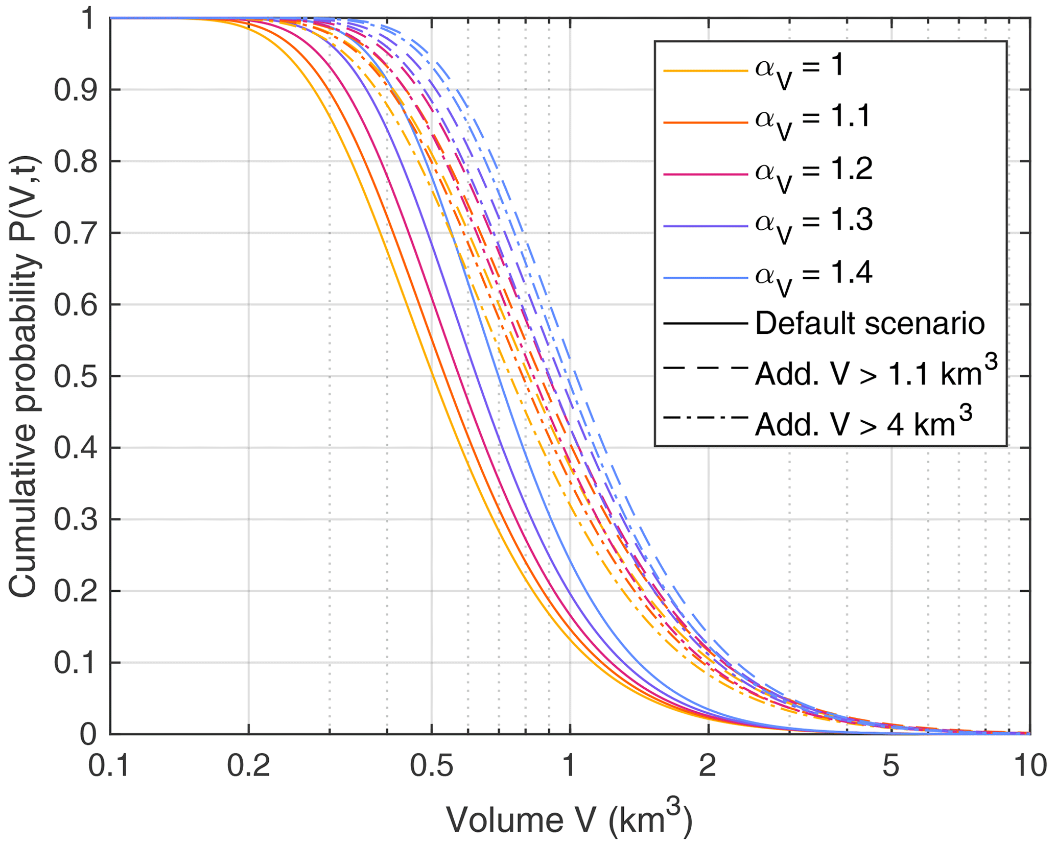
Figure 6Cumulative probability of the largest rockslide at present (2020 CE). Different line types refer to the three considered scenarios.
As already expected from Fig. 5b and c, the two scenarios with an additional large rockslide are similar. However, the median of the largest available volume is in the range between 0.74 and 1.04 km3 and thus about 1.5 times higher than for the default scenario. So the estimate of the largest volume to be expected involves two sources of uncertainty with the same order of magnitude. First, there is the inability to constrain αV sufficiently well, owing to the limited amount of data. Second, there is the potential incompleteness of the data concerning the largest events at a given time, which is here taken into account by considering the two alternative scenarios.
If we go back to the time of the Kandersteg rockslide (t = 3210 BP), the relevance of the uncertainties changes. As shown in Fig. 7, the volumes predicted for the considered values of αV differ only by about 10 %. At that time, the statistics of the largest possible rockslides are still constrained well by constraints 4–7. The predictions obtained for different values of αV start to spread when proceeding towards the recent time. In turn, the difference between the scenarios stays roughly the same. So the question of whether the Kandersteg rockslide was the largest potential event at its time or only the second-largest has a similar effect at its time as it has today.
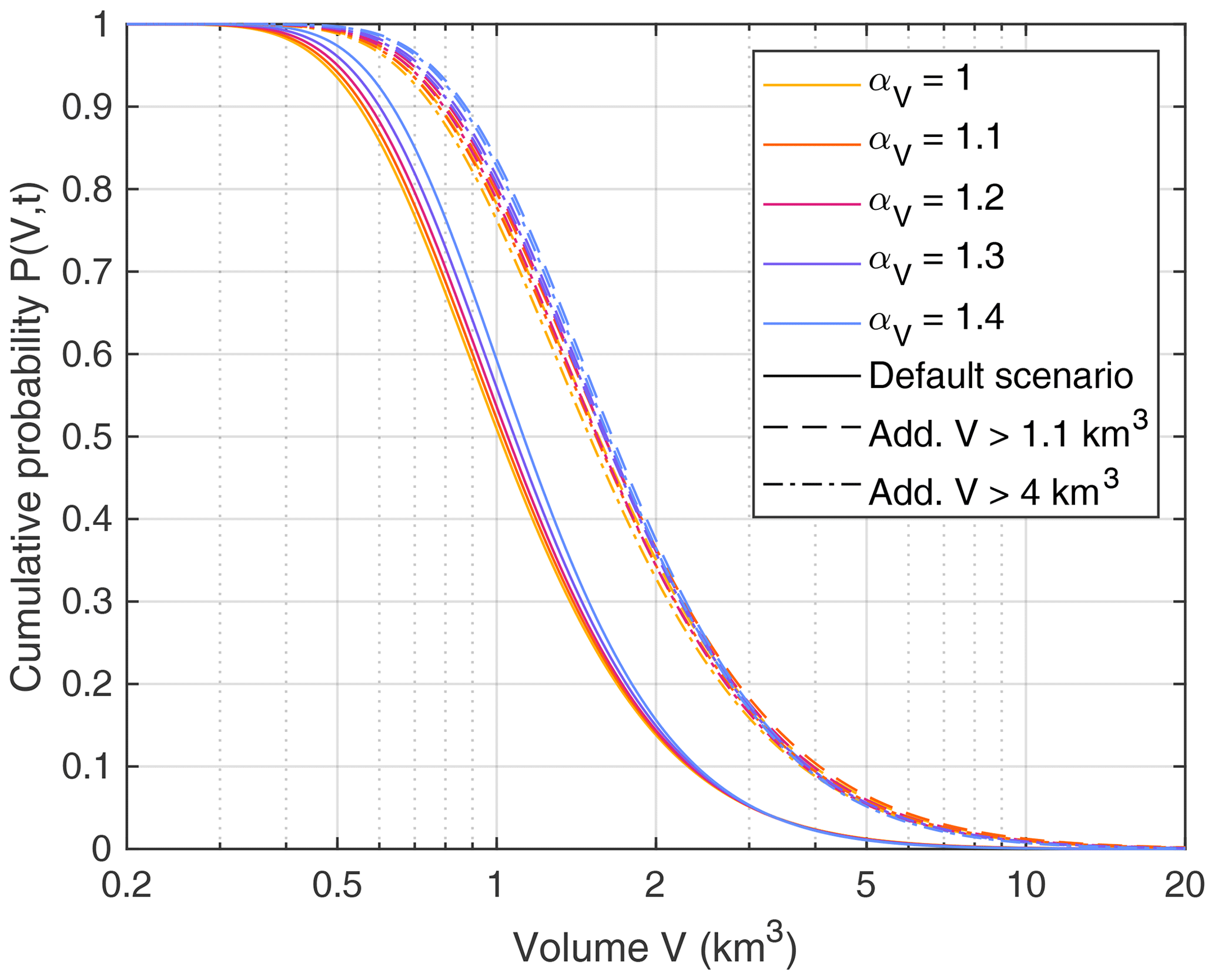
Figure 7Cumulative probability of the largest rockslide at the time of the Kandersteg rockslide (3210 BP). Different line types refer to the three considered scenarios.
As a third source of uncertainty, the statistical nature of the prediction must be taken into account. Depending on αV and on the considered scenario, the present-day 85 % and 15 % quantiles are 0.3–0.65 km3 and 0.95–2 km3, respectively (Fig. 6). So the 70 % probability range (comparable to the standard deviation of a Gaussian distribution) of the largest potential rockslide covers a factor of about 3 in volume. This uncertainty is even larger than the two other contributions to the uncertainty. It is an inherent property of the statistical distribution and would not decrease even if all parameter values (γ, μ, αV, n, and t0) were known exactly.
In all scenarios, the probability that a rockslide with V≥ 3 km3 takes place in the future is below 5 %. The probability of a rockslide with V≥ 10 km3 is even lower than 0.2 %. These results shed new light on the conclusion of von Poschinger et al. (2006) that rockslides of several cubic kilometers have to be taken into consideration also at present. Such events may be possible concerning their mechanism and the climatic conditions, but it is very unlikely that such an event would still be waiting to take place according to this framework.
In turn, the probability that there will be no rockslide with V≥ 0.24 km3 is also less than 5 % (P=0.95 in Fig. 6). This result sheds new light on the artificially triggered rockslide that struck the Vaiont reservoir in 1963 and claimed about 2000 lives. With a volume of about 0.27 km3, this rockslide cannot be considered extraordinarily large, and natural events of this size must be taken into account in the future.
Figure 8 brings the probability of occurrence into play. It shows the expected cumulative frequency F(V,t) (events per year) at present. All curves are strikingly close to each other for 5 × 10⁻⁴ km3 0.02 km3. In this range, the frequencies are constrained well by recent inventories (constraints 1 and 2).
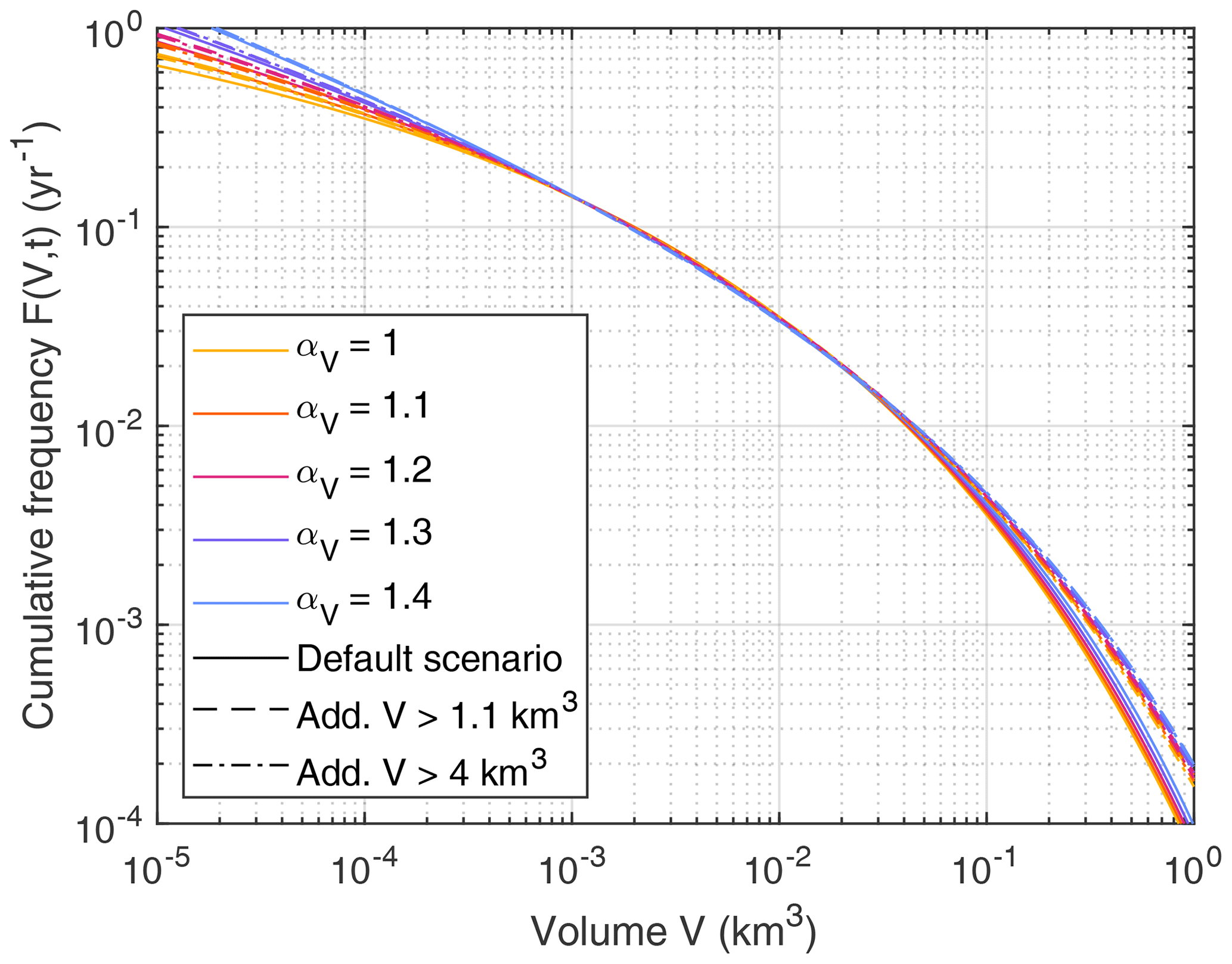
Figure 8Cumulative rockslide frequency at present (2020 CE). Different line types refer to the three considered scenarios.
The 100-year event (F(V,t) = 0.01 yr−1) has a volume of 0.04–0.045 km3. This is approximately the size of the rockslide that took place in Val Pola in 1987 (e.g., Crosta et al., 2003). In the context of large events, the 475-year event is often considered, which is the event with a probability of 10 % over 50 years. The predicted volume of this event is 0.15–0.2 km3. The predicted frequency of the size of the Vaiont rockslide (V = 0.27 km3) is between than 0.00145 yr−1 and 0.00085 yr−1, which means that a 700- to 1200-year event was triggered at the reservoir in 1963. Finally, rockslides with a volume of 1 km3 should be expected at a probability of less than 1 per 5000 years.
Let us now come back to the question of what we can learn about the process of exhaustion. Concerning the process, the exponent γ is the central parameter, while αV does not refer immediately to exhaustion, and μ, n, and t0 should depend on the considered case study. The likelihood plots shown in Fig. 5 tentatively suggest . Despite the uncertainty of this estimate, is clearly more likely than . In terms of triggering a given site from different points, this finding suggests that triggering should take place rather from the outcrop line of the failure surface (or a part of it) than from any point of the entire failure surface.
This knowledge may also be useful for validating or refuting models. So far, reproducing an exponent in the range seems to be the main goal of models of rockslide disposition. Although already challenging, this is still a rather weak criterion. In the context of SOC, it would only refer to the quasi-steady state, while the exponent γ provides additional information about the behavior if driving ceases.
However, the simulation shown in Sect. 2.2 already revealed that determining γ from simulations may be challenging. The observed concentration of the triggering points around the outlines of the predicted rockslides tentatively suggests that the model proposed by Hergarten (2012) may behave correctly, but the occurrence of overlapping events of different sizes makes a direct analysis difficult. Simulating and analyzing exhaustion starting from a quasi-steady state would be an alternative strategy of validation for comprehensive models that also include long-term driving, such as HyLands (Campforts et al., 2020).
As a fundamental property of the process of exhaustion, Fig. 9 shows the e-folding time:
For V≥ 10 km3, T is shorter than 2000 years for all scenarios. In turn, T > 65 000 yr for V≤ 10−6 km3 (1000 m3). So paraglacial exhaustion should have a minor effect on the frequency of events with V≤ 1000 m3. The e-folding time T = 5700 yr estimated by Cruden and Hu (1993) occurs in Fig. 9 in a range from V = 0.04 km3 to V = 0.5 km3, depending on the considered scenario. However, Cruden and Hu (1993) found T=5700 yr as a lumped e-folding time for an inventory with 10−6 km3 0.05 km3. So it seems that Cruden and Hu (1993) overestimated the exhaustion of small rockslides (underestimated T) perhaps due to undetected potential landslide sites.
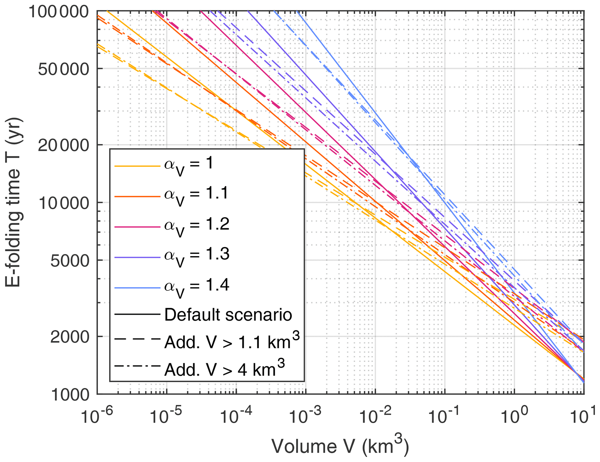
Figure 9The e-folding time of the exhaustion as a function of the volume. Different line types refer to the three considered scenarios.
From a geological point of view, the time t0 at which the process of exhaustion started might even be the most interesting parameter. As shown in Fig. 5, the likely parameter range even comprises values of t0 earlier than 15 000 BP. Such values would bring the deglaciation of the major valleys back into play. However, Fig. 10 reveals that the results become unrealistic between t0 and the time of the Flims rockslide (9450 BP). In particular for small values of αV, the approach predicts an unrealistically large number of rockslides with V≥ 10 km3 during the early phase of exhaustion. All combinations that yield a starting time t0 earlier than 15 000 BP predict more than 10 potential rockslides with V≥ 10 km3 at t = 15 000 BP, and it is very unlikely that the Flims rockslide is the only preserved one among those.
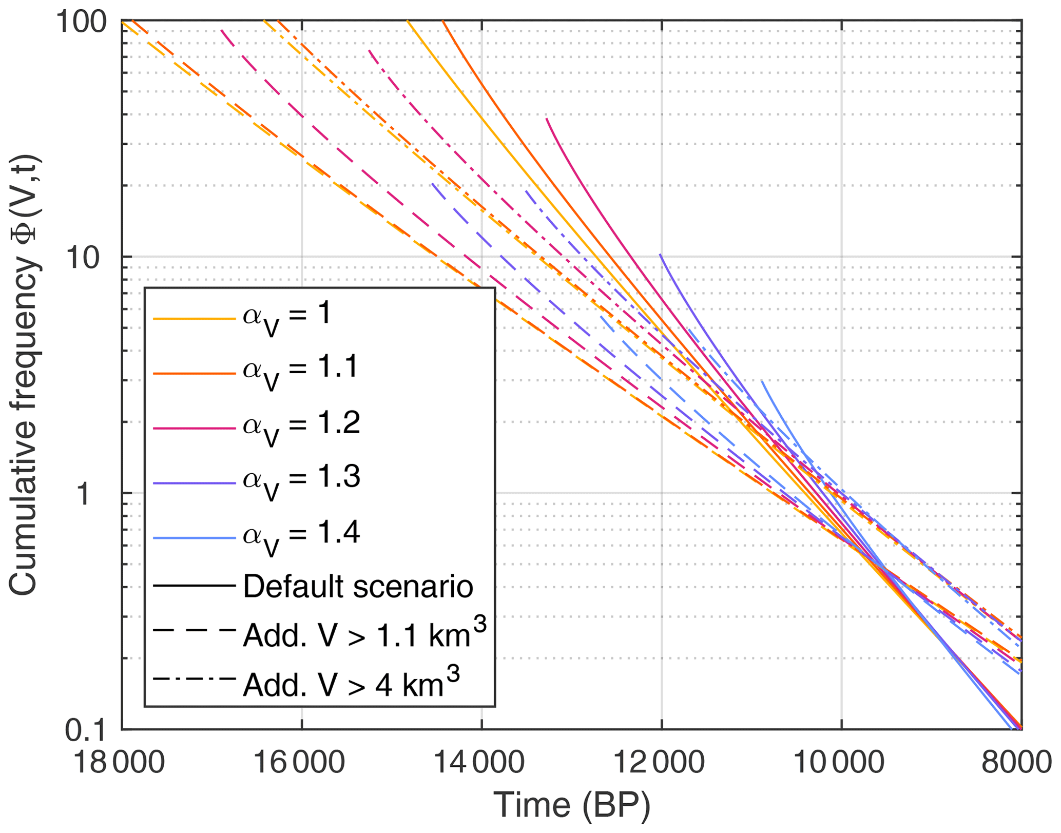
Figure 10Cumulative frequency of potential rockslide sites with V≥ 10 km3. Different line types refer to the three considered scenarios.
However, t0 is only a hypothetical time at which exhaustion started from a power-law distribution without any cutoff at large sizes. As observed in Sect. 2.1, even the quasi-steady state of the DS-FFM already shows a cutoff in the power-law distribution at large event sizes. This behavior is typical for models in the context of SOC. While the cutoff can be attributed to the finite growth rate in the DS-FFM, it is even not clear what the quasi-steady state would look like in the rockslide model discussed in Sect. 2.2. For the paraglacial exhaustion process it is, however, obvious that the initial relief imposes an upper limit on the potential rockslide volumes. So the process already must start from a power-law distribution with a cutoff. At least qualitatively, it makes sense to assume that it starts from the distribution including some exhaustion at a time later than t0 (formally, Φ(V,t) for t>0). A later starting time would correspond to a lower initial relief then. In order to estimate how much later than t0 the process started, we can make the hypothesis that there were not many paraglacial rockslides with V≥ 10 km3 in total, which means that Φ(V,t) should not be much larger than 1 for V=10 km3 at the time when the process of exhaustion started. If we assume , the process of exhaustion should have started between 12 000 BP and 10 000 BP for all scenarios in Fig. 10.
In view of this result, the deglaciation of the major valleys cannot be refuted only as an immediate trigger of the huge paraglacial landslides in the Alps but also as the start of the process of exhaustion. The starting point may, however, be the massive degradation of permafrost caused by rapid warming in the early Holocene era. For the Köfels rockslide, the potential relation to the degradation of permafrost was discussed by Nicolussi et al. (2015) and Zangerl et al. (2021). In these studies, the 2000-year time span from the beginning of the Holocene era to the rockslide was considered too long for a direct triggering. However, the concept of exhaustion only assumes that the respective sites became potentially unstable when permafrost retreated. Returning to Fig. 9, the predicted e-folding times are between 1100 and 2600 years for volumes from 4 to 10 km3. In view of this result, a time span of 2000 years to the occurrence of an actual instability is not too long.
However, the question for the actual trigger for the respective rockslides remains open. In principle, even the question of whether a unique trigger is needed is still open. Large instabilities may also develop slowly (e.g., Riva et al., 2018; Spreafico et al., 2021), and failure may finally occur without a unique trigger.
In this study, a theoretical concept for event-size-dependent exhaustion was developed. The process starts from a given set of potential events, which are randomly triggered through time. In contrast to a previous approach (Cruden and Hu, 1993), the probability of triggering depends on event size.
The concept was applied to paraglacial rockslides in the European Alps. Since available inventories cover only a quite short time span and older data are limited to a few huge rockslides, constraining the parameters involves a large uncertainty. Nevertheless, some fundamental results could be obtained.
Assuming that the probability of triggering is related to the volume V by a power law Vγ, the results indicate exponents or even slightly lower. Interpreting the dependence on volume as the possibility to initiate an event from different points, this result suggests that initiation may start rather from the outcrop line of the failure surface (or from a part of this line) than from any point of the failure surface. The exponent γ may be helpful for validating or refuting statistical or process-based models.
The concept of event-size-dependent exhaustion predicts an exponential decrease in rockslide frequency through time with a decay constant depending on V. For small rockslides with V≤ 1000 m3, the respective e-folding time is longer than 65 000 years. So the frequency of small rockslides should not have decreased much since the last glaciation. In turn, the predicted e-folding time is shorter than 2000 years for V≥ 10 km3. So the occurrence of rockslides on the order of magnitude of the Flims rockslide is unlikely at the present time. These e-folding times are, however, consistent with the idea that the process of exhaustion was initiated by the degradation of permafrost at the beginning of the Holocene epoch.
For the largest rockslide possible at the present time, different considered scenarios predict a median volume of 0.5 to 1 km3. However, the predicted frequency of such large events is low (less than 1 per 5000 years for V≥ 1 km3). The predicted 100-year event has a volume of 0.04–0.045 km3. The artificially triggered rockslide at the Vaiont reservoir (1963 CE, V=0.27 km3) can be considered a 700- to 1200-year event in this context.
In this section, a maximum likelihood approach that combines data of the two types discussed in Sect. 4 is developed.
The first type of data (constraints 1–3 in Sect. 4) refers to the number of events in a given range of sizes [s1,s2] during a given time interval [t1,t2]. The expected number N is easily obtained from the cumulative frequency Φ(s,t) of the potential events (Eq. 9) as
Then the respective factor in the likelihood is the probability that the actual number n of events occurs, which is given by the Poisson distribution
The second type of data (constraints 4–7 in Sect. 4) is described by rank-ordering statistics. The probability density of the kth largest among n events is
(Sornette, 2000, Eq. 6.4), where p(s) is the probability density of the events. Replacing p(s) by the frequency density ϕ(s)=np(s), switching to the cumulative frequency Φ(s), and joining the binomial coefficients yield
In the limit n→∞ at finite k, terms can be replaced by n. In combination with the relation , we obtain
If s was the measured property, the probability density pk(s) would already be the respective factor of the likelihood. Here, however, V is the measured property, so the likelihood is obtained by transforming pk(s) from s to V according to
with
obtained from Eq. (14). Then the likelihood is
Finally, the total likelihood is the product of the seven factors according to Eqs. (A2) and (A8).
All codes are available in a Zenodo repository at https://doi.org/10.5281/zenodo.7313868 (Hergarten, 2022). This repository also contains the data obtained from the computations. The author is happy to assist interested readers in reproducing the results and performing subsequent research.
The author has declared that there are no competing interests.
Publisher's note: Copernicus Publications remains neutral with regard to jurisdictional claims in published maps and institutional affiliations.
The author would like to thank the two anonymous reviewers for their constructive comments and Oded Katz for the editorial handling.
This open-access publication was funded by the University of Freiburg.
This paper was edited by Oded Katz and reviewed by two anonymous referees.
Aaron, J., Wolter, A., Loew, S., and Volken, S.: Understanding failure and runout mechanisms of the Flims rockslide/rock avalanche, Front. Earth Sci., 8, 224, https://doi.org/10.3389/feart.2020.00224, 2020. a, b
Alvioli, M., Guzzetti, F., and Rossi, M.: Scaling properties of rainfall induced landslides predicted by a physically based model, Geomorphology, 213, 38–47, https://doi.org/10.1016/j.geomorph.2013.12.039, 2014. a
Argentin, A.-L., Robl, J., Prasicek, G., Hergarten, S., Hölbling, D., Abad, L., and Dabiri, Z.: Controls on the formation and size of potential landslide dams and dammed lakes in the Austrian Alps, Nat. Hazards Earth Syst. Sci., 21, 1615–1637, https://doi.org/10.5194/nhess-21-1615-2021, 2021. a, b
Bak, P., Tang, C., and Wiesenfeld, K.: Self-organized criticality. An explanation of noise, Phys. Rev. Lett., 59, 381–384, https://doi.org/10.1103/PhysRevLett.59.381, 1987. a
Ballantyne, C. K.: A general model of paraglacial landscape response, Holocene, 12, 371–376, https://doi.org/10.1191/0959683602hl553fa, 2002a. a
Ballantyne, C. K.: Paraglacial geomorphology, Quaternary Sci. Rev., 21, 1935–2017, https://doi.org/10.1016/S0277-3791(02)00005-7, 2002b. a
Bennett, G. L., Molnar, P., Eisenbeiss, H., and McArdell, B. W.: Erosional power in the Swiss Alps: characterization of slope failure in the Illgraben, Earth Surf. Proc. Landforms, 37, 1627–1640, https://doi.org/10.1002/esp.3263, 2012. a
Brunetti, M. T., Guzzetti, F., and Rossi, M.: Probability distributions of landslide volumes, Nonlin. Processes Geophys., 16, 179–188, https://doi.org/10.5194/npg-16-179-2009, 2009. a, b
Bundesamt für Landestopografie swisstopo: swissALTI3D DTM 2 m, https://www.swisstopo.admin.ch/de/geodata/height/alti3d.html (last access: 17 May 2023), 2022. a
Campforts, B., Shobe, C. M., Steer, P., Vanmaercke, M., Lague, D., and Braun, J.: HyLands 1.0: a hybrid landscape evolution model to simulate the impact of landslides and landslide-derived sediment on landscape evolution, Geosci. Model Dev., 13, 3863–3886, https://doi.org/10.5194/gmd-13-3863-2020, 2020. a, b
Christensen, K., Flyvbjerg, H., and Olami, Z.: Self-organized critical forest-fire model: mean-field theory and simulation results in 1 to 6 dimensions, Phys. Rev. Lett., 71, 2737–2740, https://doi.org/10.1103/PhysRevLett.71.2737, 1993. a
Clar, S., Drossel, B., and Schwabl, F.: Scaling laws and simulation results for the self-organized critical forest-fire model, Phys. Rev. E, 50, 1009–1018, https://doi.org/10.1103/PhysRevE.50.1009, 1994. a
Crosta, G. B., Imposimato, S., and Roddeman, D. G.: Numerical modelling of large landslides stability and runout, Nat. Hazards Earth Syst. Sci., 3, 523–538, https://doi.org/10.5194/nhess-3-523-2003, 2003. a
Cruden, D. M. and Hu, X. Q.: Exhaustion and steady state models for predicting landslide hazards in the Canadian Rocky Mountains, Geomorphology, 8, 279–285, https://doi.org/10.1016/0169-555X(93)90024-V, 1993. a, b, c, d, e, f
Densmore, A. L., Ellis, M. A., and Anderson, R. S.: Landsliding and the evolution of normal-fault-bounded mountains, J. Geophys. Res., 103, 15203–15219, https://doi.org/10.1029/98JB00510, 1998. a
Deplazes, G., Anselmetti, F. S., and Hajdas, I.: Lake sediments deposited on the Flims rockslide mass: the key to date the largest mass movement of the Alps, Terra Nova, 19, 252–258, https://doi.org/10.1111/j.1365-3121.2007.00743.x, 2007. a, b
Drossel, B. and Schwabl, F.: Self-organized critical forest-fire model, Phys. Rev. Lett., 69, 1629–1632, https://doi.org/10.1103/PhysRevLett.69.1629, 1992. a
Grassberger, P.: On a self-organized critical forest fire model, J. Phys. A, 26, 2081–2089, https://doi.org/10.1088/0305-4470/26/9/007, 1993. a
Gruner, U.: Bergstürze und Klima in den Alpen – gibt es Zusammenhänge?, Bull. angew. Geol., 11, 25–34, https://doi.org/10.5169/seals-226166, 2006. a, b, c, d, e
Hartmeyer, I., Delleske, R., Keuschnig, M., Krautblatter, M., Lang, A., Schrott, L., and Otto, J.-C.: Current glacier recession causes significant rockfall increase: the immediate paraglacial response of deglaciating cirque walls, Earth Surf. Dynam., 8, 729–751, https://doi.org/10.5194/esurf-8-729-2020, 2020. a, b
Henley, C. L.: Statics of a “self-organized” percolation model, Phys. Rev. Lett., 71, 2741–2744, https://doi.org/10.1103/PhysRevLett.71.2741, 1993. a
Hergarten, S.: Topography-based modeling of large rockfalls and application to hazard assessment, Geophys. Res. Lett., 39, L13402, https://doi.org/10.1029/2012GL052090, 2012. a, b, c, d, e
Hergarten, S.: Event-size dependent exhaustion and paraglacial rockslides, Zenodo [code and data set], https://doi.org/10.5281/zenodo.7313868, 2022. a
Hergarten, S. and Krenn, R.: A semi-phenomenological approach to explain the event-size distribution of the Drossel-Schwabl forest-fire model, Nonlin. Processes Geophys., 18, 381–388, https://doi.org/10.5194/npg-18-381-2011, 2011. a, b, c
Hergarten, S. and Neugebauer, H. J.: Self-organized criticality in a landslide model, Geophys. Res. Lett., 25, 801–804, https://doi.org/10.1029/98GL50419, 1998. a
Hovius, N., Stark, C. P., and Allen, P. A.: Sediment flux from a mountain belt derived by landslide mapping, Geology, 25, 231–234, https://doi.org/10.1130/0091-7613(1997)025<0231:SFFAMB>2.3.CO;2, 1997. a
Ivy-Ochs, S., Kerschner, H., Reuther, A., Preusser, F., Heine, K., Maisch, M., Kubik, P. W., and Schlüchter, C.: Chronology of the last glacial cycle in the European Alps, J. Quaternary Sci., 23, 559–573, https://doi.org/10.1002/jqs.1202, 2008. a
Jeandet, L., Steer, P., Lague, D., and Davy, P.: Coulomb mechanics and relief constraints explain landslide size distribution, Geophys. Res. Lett., 46, 4258–4266, https://doi.org/10.1029/2019GL082351, 2019. a
Jensen, H. J.: Self-Organized Criticality – Emergent Complex Behaviour in Physical and Biological Systems, Cambridge University Press, Cambridge, New York, Melbourne, https://doi.org/10.1017/CBO9780511622717, 1998. a
Krenn, R. and Hergarten, S.: Cellular automaton modelling of lightning-induced and man made forest fires, Nat. Hazards Earth Syst. Sci., 9, 1743–1748, https://doi.org/10.5194/nhess-9-1743-2009, 2009. a, b
Lari, S., Frattini, P., and Crosta, G. B.: A probabilistic approach for landslide hazard analysis, Eng. Geol., 182, 3–14, https://doi.org/10.1016/j.enggeo.2014.07.015, 2014. a
Larsen, I. J., Montgomery, D. R., and Korup, O.: Landslide erosion controlled by hillslope material, Nat. Geosci., 3, 247–251, https://doi.org/10.1038/ngeo776, 2010. a
Liucci, L., Melelli, L., Suteanu, C., and Ponziani, F.: The role of topography in the scaling distribution of landslide areas: A cellular automata modeling approach, Geomorphology, 290, 236–249, https://doi.org/10.1016/j.geomorph.2017.04.017, 2017. a
Malamud, B. D., Morein, G., and Turcotte, D. L.: Forest fires: an example of self-organized critical behavior, Science, 281, 1840–1842, https://doi.org/10.1126/science.281.5384.1840, 1998. a
Malamud, B. D., Turcotte, D. L., Guzzetti, F., and Reichenbach, P.: Landslide inventories and their statistical properties, Earth Surf. Proc. Landforms, 29, 687–711, https://doi.org/10.1002/esp.1064, 2004. a
Mohadjer, S., Ehlers, T. A., Nettesheim, M., Ott, M. B., Glotzbach, C., and Drews, R.: Temporal variations in rockfall and rock-wall retreat rates in a deglaciated valley over the past 11 ky, Geology, 48, 594–598, https://doi.org/10.1130/G47092.1, 2020. a, b
Nicolussi, K., Spötl, C., Thurner, A., and Reimer, P. J.: Precise radiocarbon dating of the giant Köfels landslide (Eastern Alps, Austria), Geomorphology, 243, 87–91, https://doi.org/10.1016/j.geomorph.2015.05.001, 2015. a, b, c
Pastor-Satorras, R. and Vespignani, A.: Corrections to scaling in the forest-fire model, Phys. Rev. E, 61, 4854–4859, https://doi.org/10.1103/physreve.61.4854, 2000. a
Pruessner, G. and Jensen, H. J.: Broken scaling in the forest-fire model, Phys. Rev. E, 65, 056707, https://doi.org/10.1103/PhysRevE.65.056707, 2002. a
Riva, F., Agliardi, F., Amitrano, D., and Crosta, G. B.: Damage-based time-dependent modeling of paraglacial to postglacial progressive failure of large rock slopes, J. Geophys. Res.-Earth, 123, 124–141, https://doi.org/10.1002/2017JF004423, 2018. a
Schenk, K., Drossel, B., and Schwabl, F.: Self-organized critical forest-fire model on large scales, Phys. Rev. E, 65, 026135, https://doi.org/10.1103/PhysRevE.65.026135, 2002. a
Singeisen, C., Ivy-Ochs, S., Wolter, A., Steinemann, O., Akçar, N., Yesilyurt, S., and Vockenhuber, C.: The Kandersteg rock avalanche (Switzerland): integrated analysis of a late Holocene catastrophic event, Landslides, 17, 1297–1317, https://doi.org/10.1007/s10346-020-01365-y, 2020. a, b
Sornette, D.: Critical Phenomena in Natural Sciences – Chaos, Fractals, Selforganization and Disorder: Concepts and Tools, Springer, Berlin, Heidelberg, New York, https://doi.org/10.1007/3-540-33182-4, 2000. a, b
Spreafico, M. C., Sternai, P., and Agliardi, F.: Paraglacial rock-slope deformations: sudden or delayed response? Insights from an integrated numerical modelling approach, Landslides, 18, 1311–1326, https://doi.org/10.1007/s10346-020-01560-x, 2021. a
Strunden, J., Ehlers, T. A., Brehm, D., and Nettesheim, M.: Spatial and temporal variations in rockfall determined from TLS measurements in a deglaciated valley, Switzerland, J. Geophys. Res.-Earth, 120, 1251–1273, https://doi.org/10.1002/2014JF003274, 2015. a
Tanyas, H., Allstadt, K. E., and van Westen, C. J.: An updated method for estimating landslide-event magnitude, Earth Surf. Proc. Landforms, 43, 1836–1847, https://doi.org/10.1002/esp.4359, 2018. a
Tebbens, S. F.: Landslide scaling: A review, Earth Space Sci., 7, e2019EA000662, https://doi.org/10.1029/2019EA000662, 2020. a
Tinner, W., Kaltenrieder, P., Soom, M., Zwahlen, P., Schmidhalter, M., Boschetti, A., and Schlüchter, C.: Der nacheiszeitliche Bergsturz im Kandertal (Schweiz): Alter und Auswirkungen auf die damalige Umwelt, Eclogae Geol. Helv., 98, 83–95, https://doi.org/10.1007/s00015-005-1147-8, 2005. a
Valagussa, A., Frattini, P., and Crosta, G. B.: Earthquake-induced rockfall hazard zoning, Eng. Geol., 182, 213–225, https://doi.org/10.1016/j.enggeo.2014.07.009, 2014. a
von Poschinger, A., Wassmer, P., and Maisch, M.: The Flims rockslide: history of interpretation and new insights, in: Landslides from Massive Rock Slope Failure, edited by Evans, S. G., Scarascia-Mugnozza, G., Strom, A., and Hermanns, R. L., Springer, Dordrecht, https://doi.org/10.1007/978-1-4020-4037-5_18, pp. 329–356, 2006. a, b
Zangerl, C., Schneeberger, A., Steiner, G., and Mergili, M.: Geographic-information-system-based topographic reconstruction and geomechanical modelling of the Köfels rockslide, Nat. Hazards Earth Syst. Sci., 21, 2461–2483, https://doi.org/10.5194/nhess-21-2461-2021, 2021. a, b, c
Zinck, R. D. and Grimm, V.: More realistic than anticipated: A classical forest-fire model from statistical physics captures real fire shapes, Open Ecol. J., 1, 8–13, https://doi.org/10.2174/1874213000801010008, 2008. a