Assessment of subseasonal-to-seasonal (S2S) ensemble extreme precipitation forecast skill over Europe

Heavy precipitation can lead to floods and landslides, resulting in widespread damage and significant casualties. Some of its impacts can be mitigated if reliable forecasts and warnings are available. Of particular interest is the subseasonal-to-seasonal (S2S) prediction timescale. The S2S prediction timescale has received increasing attention in the research community because of its importance for many sectors. However, very few forecast skill assessments of precipitation extremes in S2S forecast data have been conducted. The goal of this article is to assess the forecast skill of rare events, here extreme precipitation, in S2S forecasts, using a metric specifically designed for extremes. We verify extreme precipitation events over Europe in the S2S forecast model from the European Centre for Medium-Range Weather Forecasts. The verification is conducted against ERA5 reanalysis precipitation. Extreme precipitation is defined as daily precipitation accumulations exceeding the seasonal 95th percentile. In addition to the classical Brier score, we use a binary loss index to assess skill. The binary loss index is tailored to assess the skill of rare events. We analyze daily events that are locally and spatially aggregated, as well as 7 d extreme-event counts. Results consistently show a higher skill in winter compared to summer. The regions showing the highest skill are Norway, Portugal and the south of the Alps. Skill increases when aggregating the extremes spatially or temporally. The verification methodology can be adapted and applied to other variables, e.g., temperature extremes or river discharge.

1 Introduction

Extreme precipitation is one of the most impactful weather-related hazards in terms of loss of lives, economic impact and number of disasters (see, e.g., the impact of storms and flood quantified in WMO, 2021). Additionally, if several extreme precipitation events occur in close succession (temporal clustering), flooding becomes more likely (Tuel et al., 2022). The successful mitigation of weather-related hazards depends on our ability to forecast them reliably. It is therefore crucial to quantify the skill of precipitation forecasts and improve the predictability of precipitation extremes for better preparedness (Merz et al., 2020).

Subseasonal-to-seasonal (S2S) prediction refers to forecasting on timescales from about 2 weeks to a season. S2S prediction has a large range of applications (White et al., 2017, 2021), including in the humanitarian sector, public health, energy, water management and agriculture. Forecast skill at this timescale is key to better managing natural hazards (Merz et al., 2020). S2S predictions aim to fill the gap between weather forecasts and seasonal outlooks (White et al., 2017). Providing skillful predictions on subseasonal or monthly timescales is challenging (Hudson et al., 2011). Unlike short-range forecasts and seasonal outlooks that have been operational for many years, the S2S timescale was until recently a “predictability desert” (Vitart et al., 2012). The scientific community working with S2S forecasts has been growing rapidly (Mariotti et al., 2018; Merryfield et al., 2020; Domeisen et al., 2022). Many research organizations actively contribute to improving S2S forecast skill, for example through the “Challenge to improve Sub-seasonal to Seasonal Predictions using Artificial Intelligence” (S2S-challenge, 2021).

Precipitation is a challenging variable to predict, and, as a result, S2S forecasts of precipitation extremes have limited skill compared to other types of hazards (see, e.g., case studies in Domeisen et al., 2022; Tian et al., 2017; Endris et al., 2021). The analysis of S2S precipitation forecast skill could allow for us to identify regions and seasons with good or bad performance of the forecast. With this information, forecast users can know where and when the forecast information is useful or if it would require further improvement (with for example post-processing, as in Specq and Batté, 2020). Skill information is also useful to identify potential sources of predictability and windows of opportunity (i.e., intermittent time periods with higher skill; Mariotti et al., 2020). Most of the existing research on S2S prediction of precipitation extremes focuses on North America (Zhang et al., 2021; DeFlorio et al., 2019), Africa (de Andrade et al., 2021; Olaniyan et al., 2018) and Asia (Yan et al., 2021; Li et al., 2019). However little is known about the skill of S2S extreme precipitation prediction over Europe (Monhart et al., 2018; Domeisen et al., 2022). The present article aims to fill this gap.

S2S forecasts are ensemble forecasts that consist of several equally probable members, i.e., runs of the same numerical model with slightly different initial conditions (World-Climate-Service, 2021). Forecast skill is typically assessed with hindcasts. Hindcasts are forecasts run for past dates over sufficiently long time periods (about 20 years) to assess the quality of the forecast and to identify and correct model biases (e.g., Huijnen et al., 2012; Manrique-Suñen et al., 2020). The goal here is to quantify S2S forecast skill for extreme precipitation events over Europe using the forecast and hindcast data from the European Centre for Medium-Range Weather Forecasts (ECMWF; Vitart, 2020), one of the most frequently used and most skillful S2S modeling systems (de Andrade et al., 2019; Li et al., 2019; Stan et al., 2022; Domeisen et al., 2022).

Common metrics to evaluate the bias and the accuracy – and hence the skill – of ensemble forecasts include the mean absolute error, the probability integral transform, the interquartile range, the continuous ranked probability score (CRPS; Hersbach, 2000; Gneiting et al., 2007; Crochemore et al., 2016; Monhart et al., 2018; Pic et al., 2022), the Brier score (Brier, 1950) and the mean square skill score (Specq and Batté, 2020). However, these metrics capture the mean behavior of a variable: most are not directly suited to verifying extreme events. The CRPS can be adapted to focus on extremes, using the threshold-weighted CRPS (Gneiting and Ranjan, 2011; Allen et al., 2021) or using extreme value theory (Taillardat et al., 2022). Another option to verify extreme events is the relative operating characteristic (ROC): it can be used to measure the ability of the ensemble forecast to identify above-normal precipitation events (Domeisen et al., 2022; Monhart et al., 2018). In this study, we transform precipitation extremes into binary “threshold exceedance events”, where the threshold is the daily-precipitation 95th percentile. The Brier score is usually employed to verify the binary forecast. However, it has limitations because of the unbalanced categories in our case. The extreme-event dataset is composed of 95 % zeros and 5 % ones. Large parts of the forecast and observation datasets match because of the large presence of “0” values (daily precipitation lower than the 95th percentile) in both datasets. To address this issue, we also use a binary loss index focusing on extremes (“1” values). We assess the extreme events by proposing and using a simple extension of the binary loss score as introduced by Legrand et al. (2022) to ensemble forecasts. This metric considers only the case of the occurrence of an extreme event in the forecast or in the observation or in both but not the non-events (see Sect. 2.3.2). This has the advantage that the score is not dominated by the correct prediction of non-events. We compare our novel skill score to the classical Brier score (Brier, 1950). To overcome the double-penalty issue (i.e., when a location or timing error in the forecast is penalized by both a false alarm and a missed event), we allow for flexibility by aggregating the forecast information in spatial and temporal windows (Ebert et al., 2013).

This article is structured as follows. Section 2 contains a description of the forecast and verification data and the methods, including the Brier score (Brier, 1950) and a binary loss index (adapted from Legrand et al., 2022). We present the results of the analysis in Sect. 3. We discuss these results, draw conclusions and give an outlook in Sect. 4.

2 Data and methods

2.1 Data

We use ECMWF's S2S precipitation hindcast data (cycle 47r2; ECMWF, 2021; Vitart, 2020; ECMWF, 2022a) from 2001 to 2020. They are composed of 11 ensemble members, initialized twice a week and run for 46 d. We focus on Europe, in the spatial box [30^∘ N, 72^∘ N] × [−15^∘ E, 49.5^∘ E]. The hindcast period covers 20 years with 2080 forecast initializations between 4 January 2001 and 30 December 2020 (twice a week, on Monday and Thursday). The data were downloaded at the model spectral resolution O320 (ECMWF, 2022b, c) and regridded for the analysis to a $\mathrm{0.5}{}^{\circ }\times \mathrm{0.5}{}^{\circ }$ regular grid using a first-order conservative remapping (Jones, 1999; CDO, 2018).

ERA5 precipitation (Hersbach et al., 2019) is used here as the verification dataset. The choice of a reanalysis dataset is motivated by its continuous spatial and temporal availability and by it avoiding the uncertainties due to the inherent spatial sparsity of weather station networks (Hofstra et al., 2009; Rivoire et al., 2021). Daily precipitation are extracted over the same time period, from 4 January 2001 to 30 December 2020 plus 46 lead time days, i.e., 14 February 2021, with a spatial resolution of $\mathrm{0.5}{}^{\circ }\times \mathrm{0.5}{}^{\circ }$. For the sake of simplicity, “observation” refers to ERA5 in the remainder.

2.2 Definition of extreme events

We define precipitation extremes as binary exceedances of daily precipitation accumulation above its 95th seasonal all-day percentile (i.e., over all days in March–April–May, MAM; June–July–August, JJA; September–October–November, SON; or December–January–February, DJF). Figure A1 in the Appendix shows the 95th percentile (Q₉₅) in ERA5 in Europe, for the period from 4 January 2001 to 14 February 2021. For the hindcast data, we also compute percentiles separately for each lead time: for a given lead time day and a given season, Q₉₅ is computed from daily precipitation of all the ensemble members pooled together. Figure 1 shows the bias in this percentile between the forecast and ERA5 data for four different lead times. In this figure and all the following ones, only values at grid points where Q₉₅ in the observations is greater than 5 mm d⁻¹ are shown. For a lead time of 1 d, the forecast generally underestimates Q₉₅. For lead times between 2 and 46 d, some regions have a positive bias (central Europe in spring and summer) and some have a negative bias (the Alps in summer, autumn and winter and Norway in spring, autumn and winter; see Fig. 1). Generally over Europe, the bias depends on the lead time and on the season. However, the bias over oceans often has the opposite sign of the bias over land.

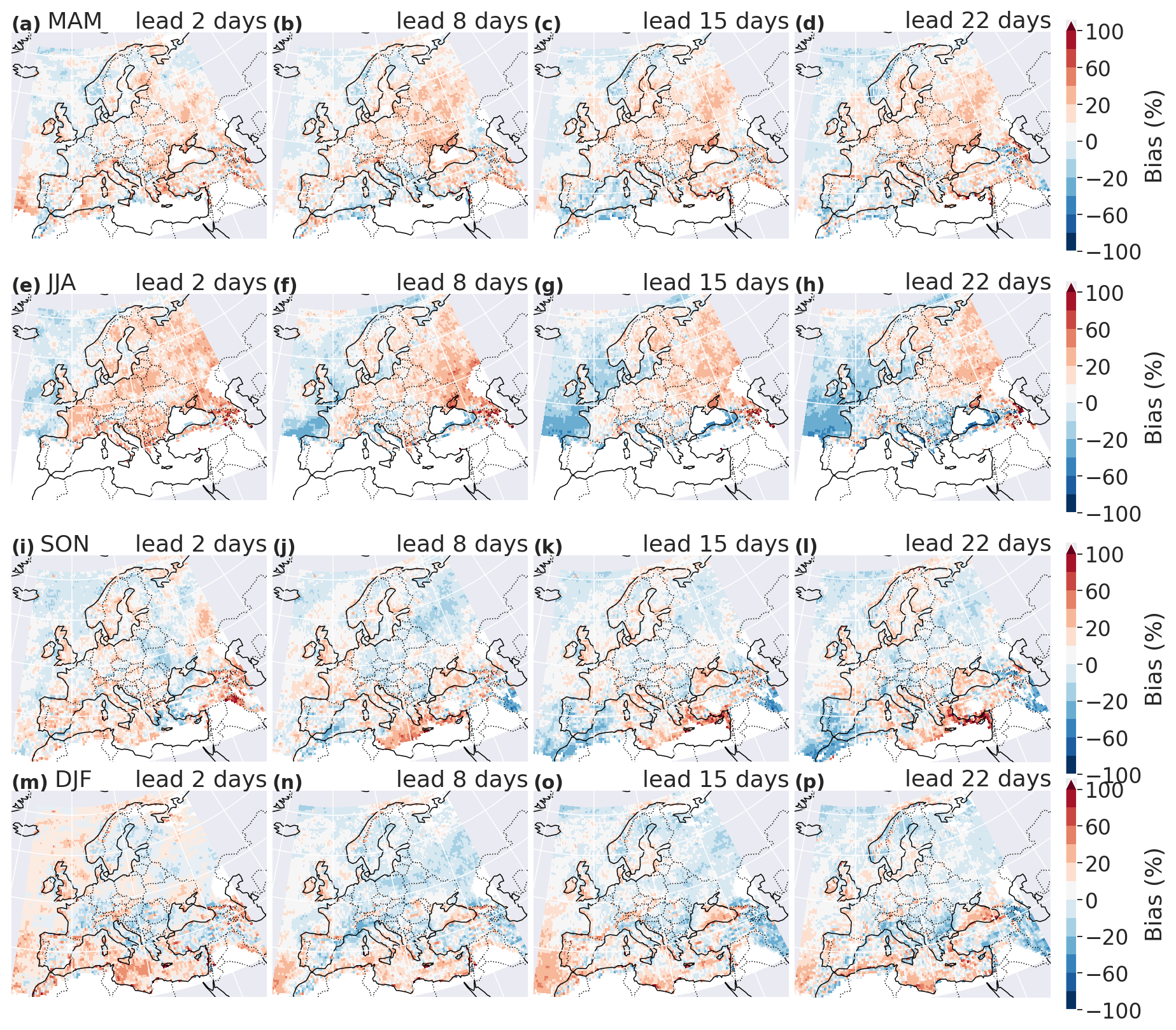
Figure 1 Forecast bias in the 95th percentile (Q₉₅) compared to ERA5, for spring (MAM, a–d), summer (JJA, e–h), autumn (SON, i–l) and winter (DJF, m–p) at a 2 d (a, e, i, m), 8 d (b, f, j, n), 15 d (c, g, k, o) and 22 d (d, h, l, p) lead time. Grid points with Q₉₅≤ 5 mm d⁻¹ are displayed in white.

2.3 Metrics

We use the Brier score and a binary loss index to assess the forecast skill in extreme events. We compute the Brier score and the binary loss index for the extended winter season (NDJFMA, i.e., November to April) and extended summer season (MJJASO, i.e., March to October). When defining the extremes (see previous section) we used 3-month-long seasons because of the strong seasonal cycle in extreme precipitation (see Fig. A1). The choice of extended seasons for the skill analysis is a compromise between having enough extreme events for a robust analysis and capturing the seasonality of the forecast. As a consequence, the probability of the extreme events is no longer exactly 0.05 if extreme events are not homogeneously distributed within the MAM and SON seasons.

2.3.1 Brier score

The Brier score B is defined as the mean square difference between forecast probability and binary observations (Brier, 1950): $B=\frac{\mathrm{1}}{n_{\mathrm{D}}}\sum _{i=\mathrm{1}}^{n_{\mathrm{D}}}(f_i-Y_i{)}^{\mathrm{2}}$, where n_D is the total number of days (i.e., the number of initializations in the given extended season: about 1040 per lead time, which is half the number of initializations per year); Y_i the binary observation of extremes for day i (Y_i=1 if the daily precipitation exceeds the 95th percentile, and Y_i=0 otherwise); and f_i is the forecast probability of extreme occurrence for day i, i.e., the mean of the ensemble members $f_i=\frac{\mathrm{1}}{M}{\sum }_{m=\mathrm{1}}^M{F}_{(i,m)}$, with M the number of ensemble members (here M=11) and F_(i,m) the binary forecast for a given ensemble member m for day i.

B is negatively oriented (the lower, the better). The climatological Brier score B_clim is used as a reference value for the skill calculation:

$$\begin{array}{}\text{(1)}& B_{\mathrm{clim}}={\displaystyle \frac{\mathrm{1}}{n_{\mathrm{D}}}}\sum _{i=\mathrm{1}}^{n_{\mathrm{D}}}(p-Y_i{)}^{\mathrm{2}},\end{array}$$

where p is the extreme-climatological-event probability. Note that the value of this probability is not exactly 0.05, as two of the 3-month seasons are split to form the extended seasons. p is therefore computed empirically.

The forecast is skillful if its Brier score is lower than the climatological Brier score. These scores can be compared using the Brier skill score (BSS):

$$\begin{array}{}\text{(2)}& \mathrm{BSS}=\mathrm{1}-{\displaystyle \frac{B_{\mathrm{hind}}}{B_{\mathrm{clim}}}}.\end{array}$$

BSS varies between $(-\mathrm{\infty },\mathrm{1}]$ and is positively oriented (the closer to 1, the better). For a given lead time day, a forecast has skill if BSS > 0. From here on, the expression “the last skillful day” refers to the largest lead time day with skill.

2.3.2 Binary loss index

Legrand et al. (2022) studied in detail a risk function defined as the ratio between (i) the empirical probability of having an extreme event in either the observation dataset or the forecast dataset and (ii) the empirical probability of having an extreme event in the observations or the forecast (including having an event in both datasets). In our context, the risk function can be written as follows:

$$\begin{array}{}\text{(3)}& R^{\left(u\right)}\left(X\right)={\displaystyle \frac{\mathbb{P}(X^{\left(u\right)}\ne Y^{\left(u\right)})}{\mathbb{P}(Y^{\left(u\right)}=\mathrm{1}\mathrm{or}{X}^{\left(u\right)}=\mathrm{1})}},\end{array}$$

where Y^(u) is the binary observation with Y^(u)=0 (Y^(u)=1) if the observed daily precipitation is lower (greater) than a certain threshold u and X^(u) is the binary forecast with X^(u)=0 (X^(u)=1) if the predicted daily precipitation is lower (greater) than u.

The risk function R^(u) focuses on how well the 1 values (extreme-event days) match between observation and forecast. It does not take into account steps when neither the forecast nor the observation experiences an extreme event. R^(u)(X) varies between [0,1] and is negatively oriented (the closer to zero, the better the forecast is). The strength of R^(u)(X) is its asymptotic behavior: even for very rare events, both the over-optimistic and over-pessimistic forecasts will be penalized. In other words, even for a very large threshold u, i.e., Y=1 for very rare occasions (but at least once), if the forecast is too optimistic and X=0 for all time steps, then R^(u)(X)=1 (“naive” classifier; Legrand et al., 2022). A very pessimistic forecast will be penalized the same way (“crying-wolf” classifier; see Legrand et al., 2022). The commonly used Brier score rather assesses the average behavior, with a very weak penalty for underrepresented classes. Because all days are compared, the assessment of rare extreme events (missed, false alarm or hit) by the Brier score is lost among the huge number of correctly predicted 0 values.

The function 1−R^(u)(X) can be understood as a critical success index for rare events (Schaefer, 1990; Legrand et al., 2022), with asymptotic properties proven by Legrand et al. (2022), such as the link to the extremal index (we refer the reader to their article for more details).

The risk function R^(u)(X) is initially designed for deterministic forecasts. We extend it here to an index for ensemble forecasts by comparing the observed exceedances with the median member of the forecast exceedances F^med. There are 11 members in the ECMWF precipitation hindcast data: for a given location, a given initialization date and a given lead time, F^med=1 if at least six ensemble members predict extreme precipitation, and F^med=0 otherwise. We take here the median forecast across members, but in practice F^med=1 could be set to 1 only if fewer or more than six members forecast extreme precipitation. The choice depends on the risk aversion of the users and is discussed in Sect. 4.

This adapted index is later on called the binary loss index (BLI_m, m indicating the median of the ensemble members). It is defined by

$$\begin{array}{}\text{(4)}& {\mathrm{BLI}}_m={\displaystyle \frac{N_{\mathrm{1}}^{\mathrm{med}}}{N_{\mathrm{2}}^{\mathrm{med}}}},\end{array}$$

where $N_{\mathrm{1}}^{\mathrm{med}}$ is the number of days when the observation and the ensemble median disagree, i.e., $N_{\mathrm{1}}^{\mathrm{med}}=\mathit{\#}\mathit{\left\{}j\right|F_j^{\mathrm{med}}\ne Y_j\mathit{\}}$, and $N_{\mathrm{2}}^{\mathrm{med}}$ is the number of days when an extreme event occurs in either the observation or the ensemble median or in both of them, i.e., $N_{\mathrm{2}}^{\mathrm{med}}=\mathit{\#}\mathit{\left\{}j\right|\left(F_j^{\mathrm{med}}=\mathrm{1}\mathrm{or}{Y}_j=\mathrm{1}\right)\mathit{\}}$. In other words, $N_{\mathrm{1}}^{\mathrm{med}}$ is the number of false positives and false negatives and $N_{\mathrm{2}}^{\mathrm{med}}$ is the number of true positives, false positives and false negatives.

To measure the lead time dependence of the skill, BLI is computed for each lead time day. Note that if the forecast F and the observation Y are independent (i.e., the forecast has no skill) and if $\mathbb{P}[F=\mathrm{1}]=\mathbb{P}[Y=\mathrm{1}]=\mathit{\alpha }$, then BLI $=\frac{\mathrm{2}-\mathrm{2}\mathit{\alpha }}{\mathrm{2}-\mathit{\alpha }}$ (here, α=0.05 for daily exceedances in a given season). In our case, ℙ[F=1] is not exactly equal to ℙ[Y=1] because the index is computed on extended seasons and not on 3-month seasons.

The climatological value of BLI, referred to as BLI_clim, is used as reference value. We compute confidence intervals for BLI_clim with a bootstrap procedure to determine if the forecast is skillful, i.e., if BLI is significantly lower than BLI_clim. For a given bootstrap step, a random time series is formed by drawing values in the observation time series. BLI is computed with this random time series as the forecast. For a given lead time day, a forecast is deemed to be significantly skillful if the BLI of the median member of the forecast (F^med) is lower than the 5th percentile of the confidence interval on BLI_clim. Like for the Brier score, we compute the “last skillful day” for BLI, with the same definition (largest lead time day with skill; see Fig. 2 for an example).

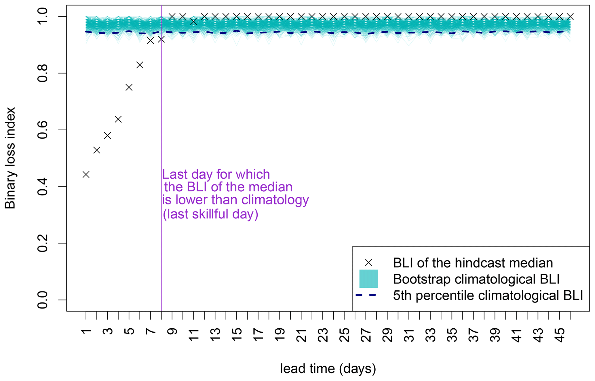
Figure 2 Definition of the last skillful day for BLI: example for one grid point and one season.

2.3.3 Spatio-temporal extension of the metrics

Requiring an exact match of events in the forecast and the observations on the same day and at the same grid point is very strict. Indeed, precipitation is a complex variable to forecast precisely in space and time. A forecast may contain useful information, even if the forecast does not predict the event exactly on the same day or at the same location as in the observation but in a close neighborhood. Moreover, a temporal lag or a spatial shift between the observation and the forecast is penalized twice, by (1) a missed event at the observed time/location of the event and (2) a false alarm at the erroneously predicted time/location of the event (double-penalty issue; see, e.g., Ebert et al., 2013). We therefore also compute skill scores on data aggregated in space and time, which allows for some flexibility in the exact location or exact timing of the events. The spatial and the temporal aggregations are conducted independently to analyze the individual impact of each aggregation. Both the spatial and the temporal neighborhoods are non-overlapping to consider each extreme event only once. The spatio-temporal extensions are applied before computing the median member.

The temporal aggregation consists in counting the number of extreme events N^t in a 7 d window. We then translate it into a binary series $E_n^t$, given a minimum number of events n in the window ($n=\mathit{\{}\mathrm{1},\mathrm{\dots },\mathrm{7}\mathit{\}}$):

$$\begin{array}{}\text{(5)}& E_n^t=\left\{\begin{array}{ll}\mathrm{1}& \text{if}{N}^t\ge n\\ \mathrm{0}& \text{otherwise.}\end{array}\right.\end{array}$$

Figure 3 provides an example for the definition of $E_n^t$. To the various binary series (one for each n value), we apply the Brier score and BLI to quantify forecast skill. We estimate climatological skill in a way that conserves the temporal structure of the climatology. We randomly select the beginning of the 7 d time windows in the observation. The following 6 d is not randomly selected; it is the 6 d actually following the beginning of time window in the time series of observations.

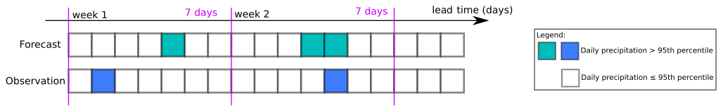
Figure 3 Illustration of the weekly aggregation of extremes at one grid point. During week 1, the forecast predicts one extreme and one extreme is observed. For both the forecast and the observation, the number of extreme events in the 7 d window is greater than or equal to 1: $E_{\mathrm{1}}^t=\mathrm{1}$ for the two datasets. For both datasets, the number of events in the 7 d window is lower than n for n≥2: $E_n^t=\mathrm{0}$ for the two datasets. During week 2, one extreme is observed but the forecast predicts two events. For both datasets, the number of extreme events in the 7 d window is greater than or equal to 1: $E_{\mathrm{1}}^t=\mathrm{1}$ for the two datasets. For the observation, the number of events in the 7 d window is lower than 2 ($E_{\mathrm{2}}^t=\mathrm{0}$), and this number is greater than or equal to 2 for the forecast ($E_{\mathrm{2}}^t=\mathrm{1}$). For the configuration with n≥3, $E_n^t=\mathrm{0}$ for both datasets.

The spatial aggregation is performed by counting extreme precipitation events in neighborhoods. Like for the temporal aggregation, we define two categories, depending on whether or not the count of events N^s in the spatial neighborhood exceeds some threshold n (see Fig. 4 for an example):

$$E_n^s=\left\{\begin{array}{ll}\mathrm{1}& \text{if}{N}^s\ge n\\ \mathrm{0}& \text{otherwise.}\end{array}\right.$$

Precipitation includes some spatial structure, i.e., spatial dependence between points in a neighborhood. When computing the climatology for both scores, the spatial structure is conserved: for one step of the bootstrap, only the date is randomly chosen, and the spatial neighborhood is the observed neighborhood for that day. We define the neighborhoods as square boxes of about 150 km × 150 km, i.e., boxes with a latitudinal extent of 1.5^∘ N (three grid boxes) and with a longitudinal grid extent that depends on the latitude: from 1.5^∘ E at 30^∘ N (three grid boxes) to 4.5^∘ E at 70^∘ N (nine grid boxes); see Fig. D1 in the Appendix for an illustration.

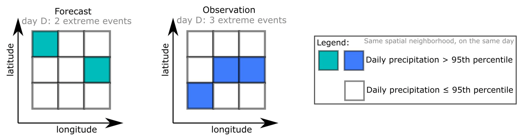
Figure 4 Illustration of the spatial aggregation of extremes in one neighborhood. The forecast indicates two extremes in the spatial neighborhood, and three events are observed. For both datasets, the number of extreme events in the neighborhood is greater than or equal to 1 ($E_{\mathrm{1}}^s=\mathrm{1}$) and greater than or equal to 2 ($E_{\mathrm{2}}^s=\mathrm{1}$). For three events or more, $E_{\mathrm{3}}^s=\mathrm{0}$ for the forecast and $E_{\mathrm{3}}^s=\mathrm{1}$ for the observation. For four events or more, $E_n^s=\mathrm{0}$ for both datasets.

3 Results

3.1 Daily and local comparison

We begin by discussing the forecast skill at the daily and grid-point scale. BLI indicates more skill during the extended winter (skill for up to 11 d and many regions with a last skillful day greater than 7 d) than during the extended summer (last skillful day below 6 d for most grid points); see Fig. 5. Regions with high skill are Norway, the Alps and the western half of the Iberian Peninsula in the extended winter and the Bay of Biscay, the south of France, Norway, central Europe and the south of the Alps in the extended summer. The BLI skill score is less conservative than the Brier skill score; however the spatial patterns are similar for the two metrics (Fig. B1 in the Appendix). That is, the last skillful day for the Brier skill score is overall smaller than the last skillful day for BLI, but both the Brier score and BLI show the same regions with high and low skill of the forecast for precipitation extremes, in summer and winter.

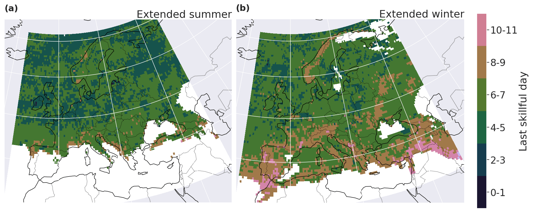
Figure 5 Last skillful day for BLI for a local and daily comparison, in extended summer (a) and extended winter (b).

3.2 Temporal aggregation

The 7 d extreme-precipitation-event counts are also better predicted during the extended winter than during the extended summer (Fig. 6). For the category “one event or more occurred during the 7 d”, the forecasts at most grid points still have skill for lead times into the second week, i.e., days 8–14, in extended winter. BLI decreases as the number of events per week increases; however, the spatial patterns remain the same. The regions where temporal clustering is more skillfully forecasted are the Iberian Peninsula, Norway and the northern Mediterranean coastline (especially in winter). The Brier score confirms these results, with similar patterns (see Fig. C1 in the Appendix).

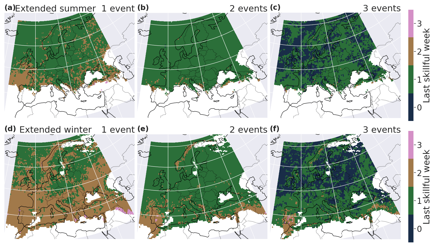
Figure 6 Last week of skill for BLI in extended summer (a–c) and extended winter (d–e) for a minimum of one (a, d), two (b, e) and three (c, f) events in a 7 d window. A last skillful week equal to 0 means that, for the count of extremes during the first-week lead time, BLI of the forecast is not significantly lower than BLI_clim.

3.3 Spatial aggregation

Extended winter forecasts for spatially aggregated extremes are also more skillful than summer ones (see Fig. 7). The last skillful day is greater when spatially aggregating that for the local analysis, but the two configurations have a similar spatial pattern. In extended winter, for one event or more in the neighborhood, the last skillful lead time reaches up to 11 d in many regions: the western Iberian Peninsula, the Norway coast and the west-facing coasts in general. In extended summer, the last skillful lead time is between 8 and 11 d on the Atlantic coast of France, Italy, western Europe and the coasts of the Iberian Peninsula. The spatial skill pattern remains similar with an increasing number of events per neighborhood, but the skill decreases.

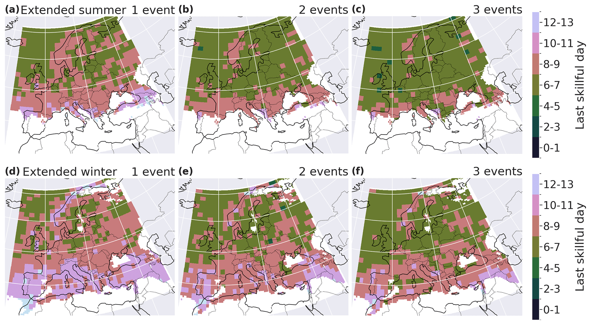
Figure 7 Last day of skill for BLI in extended summer (a–c) and extended winter (d–f) for a minimum of one (a, d), two (b, e) and three (c, f) events in neighborhoods of 150 km × 150 km.

Figure D2 in Appendix shows maps of the last lead time day with a positive Brier skill score, for different numbers of events aggregated spatially, in extended summer and extended winter. The regions with higher skill are the same for the Brier score and for BLI. The spatial pattern of the skill also remains similar with an increasing number of events per neighborhood.

4 Discussion and conclusion

In this paper, we assess forecast skill of extreme precipitation occurrence over Europe in the ECMWF S2S model. Extremes are defined as exceedances over the seasonal 95th percentile. We conduct a verification against ERA5 precipitation with the binary loss index (BLI) and the Brier score. We extend the binary loss score studied by Legrand et al. (2022), which was designed for deterministic forecasts only, to ensemble forecasts. We define BLI as the binary loss score calculated for the ensemble median member of binary exceedances. The choice of the median member was motivated by a trade-off between false alarms and missed events. The skill will be different when one chooses a lower percentile of the ensemble members to compute BLI (risk-averse setting) or when one chooses a high percentile of the ensemble members (risk-loving). BLI has the advantage of focusing exclusively on extreme-event occurrence (hit, false alarm or miss) and is not biased by the high counts of extreme-event non-occurrence. BLI is qualitatively compared with the Brier score; the skill scores of the two metrics agree very well over Europe. Despite the great importance of accurately forecasting rare extremes, the Brier score does not give a special weight to underrepresented classes. Therefore, by design, BLI should be preferred to the Brier score when assessing the forecast skill for very rare events. With further research, a probability score for ensemble forecasts could be developed from BLI.

The S2S forecasts have overall higher skill in predicting extreme precipitation events in winter than in summer. A likely explanation resides in the fact that precipitation over Europe mainly results from large-scale processes during winter but from small-scale convective events in summer. Predicting small-scale events is indeed more challenging than predicting large-scale ones (Haylock and Goodess, 2004; Kenyon and Hegerl, 2010). This result is in agreement with the existing literature on S2S prediction in other regions (Tian et al., 2017; Kolachian and Saghafian, 2019). Norway, Portugal and the south of the Alps are regions with the most skill. The orography seems to be a source of skill (like in Norway, the Pyrenees and the south of the Alps): the forecast seems to better capture precipitation events where the complex topography acts as a forcing for precipitation. The Mediterranean region exhibits relatively good skill in winter. Similarly, coastal regions in general have a higher skill compared to continental regions. A potential explanation for this difference is that the water transported from the ocean first rains next to the coast; it is more challenging to predict where the remaining water in the atmosphere will rain down on continental regions because land–atmosphere interactions introduce uncertainty. A follow-up study could further investigate these hypotheses on the physical reasons behind the spatial and seasonal heterogeneity of the skill.

Allowing for temporal or spatial flexibility in the evaluation of the forecast extremes confirms the skill patterns, bringing robustness to the analysis. The skill for the spatially aggregated precipitation is slightly larger than for the local analysis, as it is easier for the forecast to have an event that matches with observation on a larger grid. The spatial aggregation conducted here could be adapted for an impact-oriented analysis, by aggregating, e.g., over catchments to evaluate the predictability of heavy precipitation that can potentially result in floods or by analyzing multi-day heat waves.

We additionally investigated the effect of European weather regimes on the forecast skill (as defined in Grams et al., 2017), as the forecast skill of the weather regimes themselves can largely differ (Büeler et al., 2021). We computed the forecast skill independently for positive phases and negative phases of the North Atlantic Oscillation (NAO). The forecast skill does not exhibit a strong dependence on the NAO phase, although the data were also spatially aggregated to increase robustness (not shown). This absence of signal should be confirmed with a deeper analysis, by considering some time lag or seasonality for the influence of the teleconnection patterns (Tabari and Willems, 2018) or by aggregating over larger spatio-temporal neighborhoods, to increase the robustness. Other teleconnection patterns could be investigated, such as Scandinavian and eastern Atlantic patterns, El Niño–Southern Oscillation, the Atlantic Multidecadal Oscillation (Casanueva et al., 2014), or the state of the stratosphere (Domeisen et al., 2019).

An assessment focused on the precipitation intensity could extend the verification; the precipitation forecast data would then require calibration (Gneiting et al., 2007; Specq and Batté, 2020; Crochemore et al., 2016; Monhart et al., 2018; Huang et al., 2022). An extension of the CRPS would be an option to measure the intensity forecast skill with a focus on heavy precipitation, like the threshold-weighted CRPS (see, e.g., Pantillon et al., 2018; Allen et al., 2021) or using extreme value theory (Taillardat et al., 2022). Post-processing the hindcast data and analyzing the paradigm of “maximizing the sharpness of the predictive distributions subject to calibration” could also be an extension of this work (Gneiting et al., 2007); the usual evaluation metrics – the probability integral transform histogram, marginal calibration plots, the sharpness diagram – could be applied with a focus on extremes.

Note that for practical applications, one needs caution to interpret the skill in an absolute way for two reasons: (i) a skillful forecast does not mean that the forecast is also a useful forecast for practical applications and (ii) the absolute last skillful day depends on the choice of the member for the daily predictor (here, the median member). (i) If BLI is equal to 0.8 but is outside of the climatological confidence interval, the forecast is better than the climatology and therefore skillful. However, it also means that only 25 % of the extremes are caught by the forecast (by simple transformation of BLI $=\frac{\mathrm{FN}+\mathrm{FP}}{\mathrm{TP}+\mathrm{FN}+\mathrm{FP}}=\mathrm{0.8}$, where FN denotes the false negatives, FP the false positives and TP the true positives). For 75 % of the time, the forecast either erroneously predicted an extreme (false alarm, FP) or did not predict an extreme that occurred (miss, FN). The definition of the last skillful day can be adapted depending on the usage of the forecast. The definition can be more conservative, e.g., using the last lead time day for which at least 75 % of the extreme events are caught (rather than a comparison to the climatology) or using a smaller percentile of the members rather than the median member. (ii) The last skillful day is larger when choosing the maximum member as the daily predictor (i.e., F^med=1 if at least 1 ensemble member predicts extreme precipitation, and F^med=0 otherwise). This is due to the number of TPs not collapsing to zero with increasing lead times: the condition “at least one member predicts daily precipitation is greater than the 95th percentile” is very easily satisfied. By “chance”, the maximum member predicts many TPs, still compensating a bit for the FPs for large lead times. For the choice of the member, we recommend considering a good balance between FNs and FPs. However, it is important to note that the spatial pattern of skill does not depend on the choice of the member. The regions with a relatively large skill (e.g., Norway, Portugal, west coasts in winter) remain the same, independently of the choice of predictor (minimum, median or maximum member). Following these two remarks, we emphasize that our aim here was to provide a robust qualitative assessment by identifying regions of skill and challenging regions for the forecast model to predict precipitation extremes on the S2S timescale.

Checking if a value of BLI is significant is a kind of hypothesis test that is repeated for a large number of grid points. One could argue that some regional significance should be investigated. However, when displaying the local significance as “largest lead time day with skillful forecast”, the results are continuous rather than a strict “yes or no” response. Moreover, the spatial coherence of the results confirms the robustness of the method.

Our method to assess extremes can also be applied to other variables, such as consecutive days of high temperature, river discharge, etc. Considering the other end of extremes, evaluating the skill of forecasts to predict droughts is also of crucial importance. For droughts, the persistence of dry periods matters, rather than the occurrence of precipitation. The method could be adapted accordingly, e.g., by adjusting the definition of temporal aggregation introduced in this study.

Appendix A: The 95th percentile

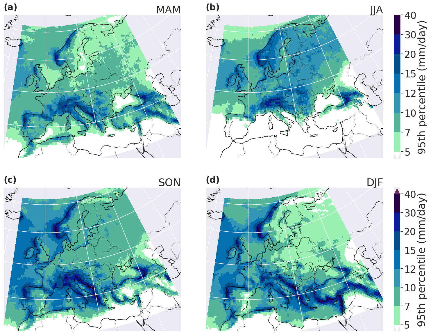
Figure A1 The 95th percentile of daily precipitation in ERA5, 2001–2021.

Appendix B: Local and daily comparison of extremes

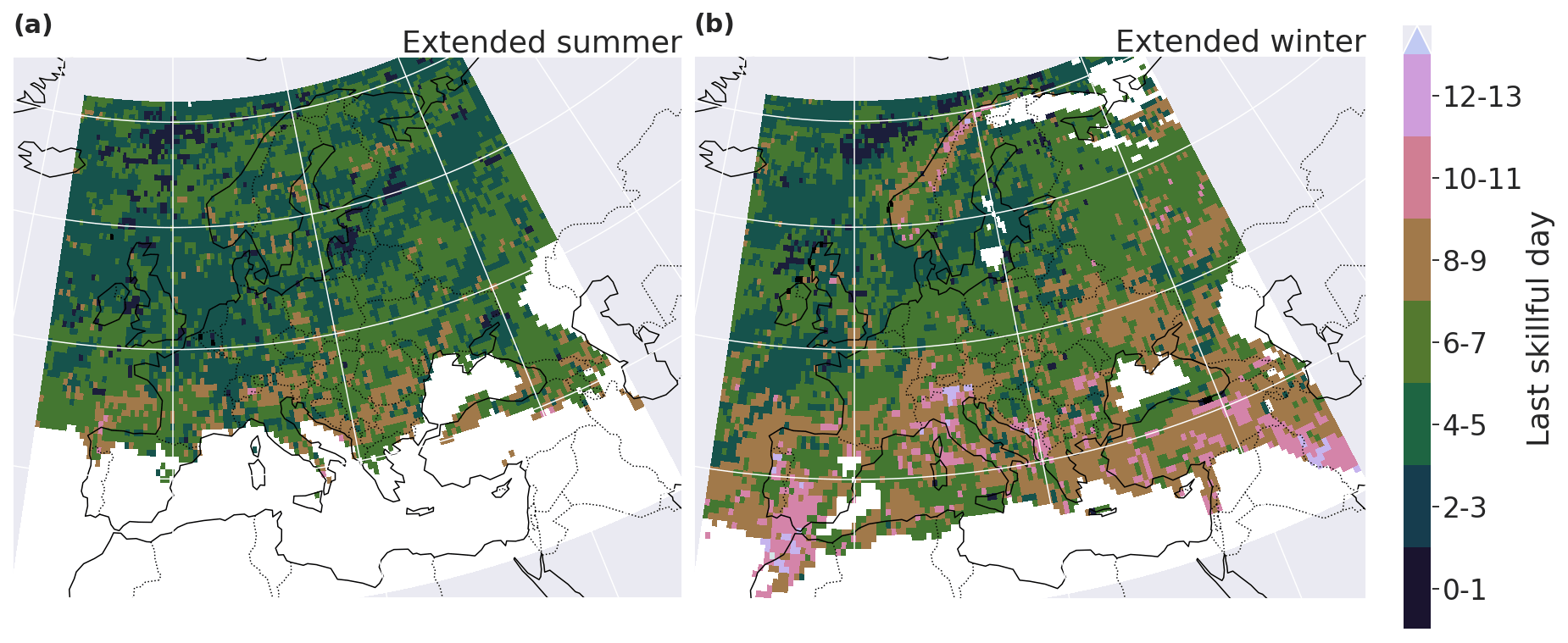
Figure B1 Last skillful day for the Brier skill score for local and daily comparison, in extended summer (a) and extended winter (b).

Appendix C: Temporally accumulated extremes

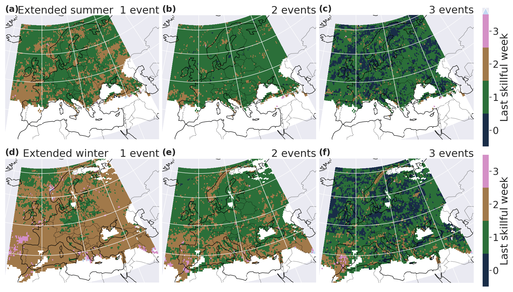
Figure C1 Last week of skill for the Brier skill score in extended summer (a–c) and extended winter (d–f) for a minimum of one (a, d), two (b, e) and three (c, f) events in a 7 d window.

Appendix D: Spatially accumulated extremes

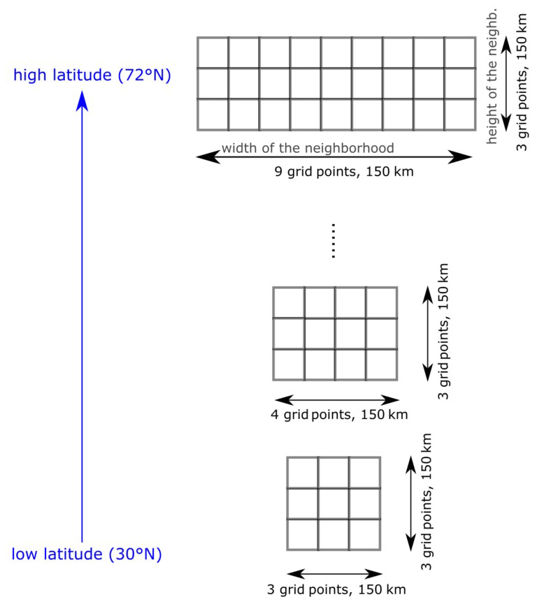
Figure D1 Illustration of the width of the spatial neighborhood, in terms of grid points, depending on the latitude for a constant width in kilometers (and for a constant area).

Brier score with spatial aggregation

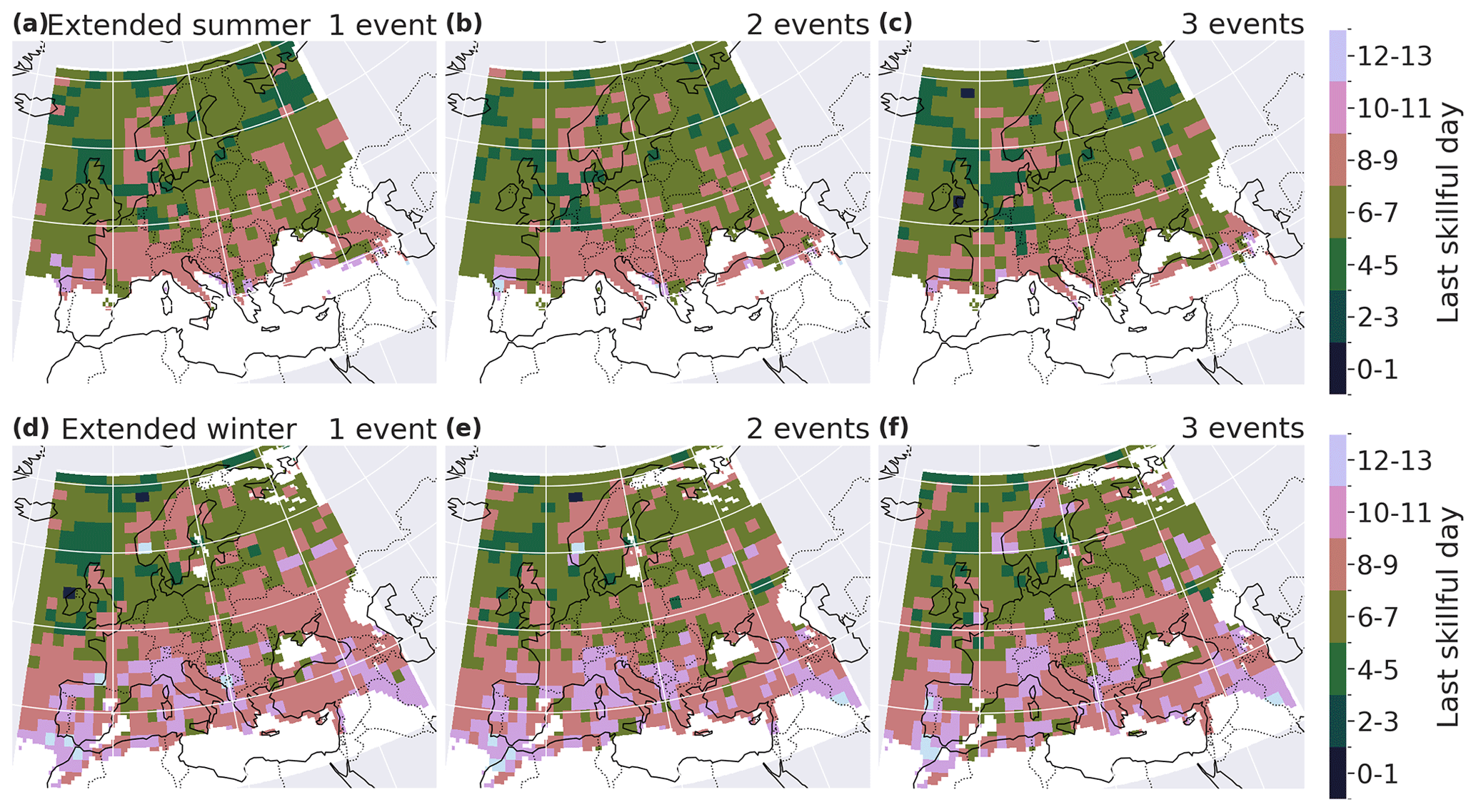
Figure D2 Last day of skill for the Brier skill score in extended summer (a–c) and extended winter (d–f) for a minimum of one (a, d), two (b, e) and three (c, f) events in neighborhoods of 150 km× 150 km.