Time of emergence of compound events: contribution of univariate and dependence properties

Many climate-related disasters often result from a combination of several climate phenomena, also referred to as “compound events’’ (CEs). By interacting with each other, these phenomena can lead to huge environmental and societal impacts, at a scale potentially far greater than any of these climate events could have caused separately. Marginal and dependence properties of the climate phenomena forming the CEs are key statistical properties characterising their probabilities of occurrence. In this study, we propose a new methodology to assess the time of emergence of CE probabilities, which is critical for mitigation strategies and adaptation planning. Using copula theory, we separate and quantify the contribution of marginal and dependence properties to the overall probability changes of multivariate hazards leading to CEs. It provides a better understanding of how the statistical properties of variables leading to CEs evolve and contribute to the change in their occurrences. For illustrative purposes, the methodology is applied over a 13-member multi-model ensemble (CMIP6) to two case studies: compound wind and precipitation extremes over the region of Brittany (France), and frost events occurring during the growing season preconditioned by warm temperatures (growing-period frost) over central France. For compound wind and precipitation extremes, results show that probabilities emerge before the end of the 21st century for six models of the CMIP6 ensemble considered. For growing-period frosts, significant changes of probability are detected for 11 models. Yet, the contribution of marginal and dependence properties to these changes in probabilities can be very different from one climate hazard to another, and from one model to another. Depending on the CE, some models place strong importance on both marginal properties and dependence properties for probability changes. These results highlight the importance of considering changes in both marginal and dependence properties, as well as their inter-model variability, for future risk assessments related to CEs.

1 Introduction

In September 2017, heavy rainfall and storm surge associated with Hurricane Irma resulted in record-breaking floods in Jacksonville, Florida. In 2019, Australia experienced high temperatures and prolonged dry conditions, which resulted in one of the worst bush fire seasons in its recorded history. In April 2021 and 2022, Central Europe experienced consecutive days of frost events following a warm early spring, which caused severe damage to agricultural yields. These recent climate events are some examples of so-called compound events (CEs), i.e. high-impact climate events that result from interactions of several climate hazards. These climate hazards are not necessarily extremes themselves, but their simultaneous or successive occurrences can generate strong impacts (Leonard et al., 2014; Zscheischler et al., 2014, 2018, 2020). Although still in its infancy, the understanding of the complex nature of CEs and the assessment of their associated risks have been the subject of numerous research studies in climate sciences (e.g. Bevacqua et al., 2017, 2021; Manning et al., 2018; Zscheischler and Seneviratne, 2017; Ridder et al., 2021, 2022; Singh et al., 2021a; Nasr et al., 2021; Raymond et al., 2022, among many others). Recently, a typology of CEs has been proposed in order to categorise them into four classes depending on how individual hazards interact to form the CEs (“preconditioned”, “multivariate’’, “temporally compounding’’ and “spatially compounding’’ events; see Zscheischler et al., 2020). Concerning projected changes, the frequency and intensity of some CEs such as co-occurring heatwaves and droughts are expected to increase for many regions of the world, even when considering climate change scenarios with limited global warming to 1.5 ^∘C above pre-industrial levels (IPCC, 2023). Determining whether the probabilities of compounding climate events present significant changes between past and future periods and detecting when these significant changes occur are of paramount importance, not only for mitigation and adaptation issues but also for informing the general public and raising awareness of climate change. Only when the changes of probability are of sufficient magnitude relative to a baseline period can we be confident that significant changes have been detected. Detecting from which period the changes are statistically significant corresponds to the concept of “time of emergence” (ToE). It consists in determining the time or period in which a climate signal emerges from (i.e. goes out of) the natural variability (e.g. Christensen et al., 2007; Maraun, 2013; Hawkins et al., 2020; Ossó et al., 2022). ToE has been discussed extensively to analyse the emergence of mean temperatures (e.g. Hawkins and Sutton, 2012; Mahlstein et al., 2011), precipitation (Fischer et al., 2014; Giorgi and Bi, 2009; Gaetani et al., 2020), but also emergence of extremes (e.g. Diffenbaugh and Scherer, 2011; Fischer et al., 2014; King et al., 2015). Evaluating the ToE of compound hazard probabilities with respect to a baseline period – from which the natural variability is estimated – is valuable for the analysis of the evolution of CEs and for attributing this to a specific cause, such as anthropogenic greenhouse gas emissions. Detection and attribution represent an important research field in climate science that aims to determine the mechanisms responsible for recent global warming and related climate changes (e.g. Bindoff et al., 2013). For example, it can be done by comparing probabilities of an event between two worlds with different forcings (the “risk-based” approach; Stott et al., 2004; Shepherd, 2016). Generally, a factual world with anthropogenic climate change and a counterfactual world in which anthropogenic emissions had never occurred are considered. Although we do not aim at performing attribution per se in the present study, the underlying philosophy is relatively similar for ToE: by considering a pre-industrial period as baseline, compound hazard probabilities associated with natural forcings – or natural variability – may be estimated, and thus also the influence of future climate change on probabilities.

From a statistical point of view, CEs are characterised by the statistical features of the variables forming the CEs, i.e. their marginal properties (e.g. mean and variance) and dependence structures. These key statistical properties can be affected by future climate change (e.g. Wahl et al., 2015; Schär, 2015; Russo et al., 2017; Raymond et al., 2020; Jézéquel et al., 2020). In addition to potentially exacerbating impacts, these changes in marginal and dependence properties could also combine to change the probabilities of the CE hazards (e.g. Rana et al., 2017; Zscheischler and Seneviratne, 2017; Zscheischler and Lehner, 2021; Manning et al., 2019; Singh et al., 2021a). For example, rising temperatures can naturally lead to more co-occurrences of hot temperatures and meteorological droughts, despite no significant trends in meteorological droughts being detected (Diffenbaugh et al., 2015; Mazdiyasni and AghaKouchak, 2015). However, in addition to warmer temperatures, the strengthening of the dependence between hot temperatures and meteorological droughts for future periods can also contribute to an increase in their co-occurrences (as highlighted in Zscheischler and Seneviratne, 2017). Several studies concluded on the importance of considering dependencies to assess CE properties and frequencies in a robust way, e.g. for wind and precipitation extremes (e.g. Hillier et al., 2020), or temperature and precipitation (e.g. Singh et al., 2021a; Vrac et al., 2022a). Recently, Abatzoglou et al. (2020) even showed that, in recent decades, changes in multivariate annual climatic conditions (water deficit, evapotranspiration, minimum and maximum temperature) with respect to a reference climate state have been more important than changes in univariate annual climatic conditions for a large portion of the Earth. Hence, to determine the ToE of hazard probabilities, quantifying the influence (or contribution) of the statistical features of the variables forming the CEs on these changes of probabilities is crucial in order to further understand the potential future evolution of CEs (Vrac et al., 2022a).

In this paper, we propose a new methodology to assess the ToE of CE probabilities. We also develop a copula-based multivariate framework, which allows for an adequate description of the contribution of the changes in marginal and dependence properties to the evolution of multivariate hazard probabilities. This CE analysis is applied to two case studies. Please note that the goal of the paper is not to provide precise results of ToE in these two case studies, but rather to introduce the conceptual framework and raise awareness among climate scientists on the potential emergence of CE probabilities, as well as the contributions of statistical properties to probability changes. We first analyse compound wind and precipitation extremes over the coastal region of Brittany (France). This bivariate CE, i.e. composed of co-occurring climate hazards over the same region and time, has been analysed in several studies (e.g. Martius et al., 2016; Bevacqua et al., 2019; De Luca et al., 2020a; Reinert et al., 2021; Messmer and Simmonds, 2021) as it can have severe impacts such as important economic losses, massive damage to infrastructure and loss of human life (e.g. Fink et al., 2009; Liberato, 2014; Wahl et al., 2015; Raveh-Rubin and Wernli, 2015). We then apply our methodology to a second climate hazard: frost events occurring during the growing season preconditioned by warm temperatures (growing-period frost) over central France. When occurring after bud burst, i.e. when the sensitive emerging leaves and flowers have started to develop, frost temperatures potentially affect the growth and distribution limits of plants. It can consequently cause important economic losses to agriculture (Lamichhane, 2021). These growing-period frost events and their associated risks in past and future periods have been studied in the literature (e.g. Unterberger et al., 2018; Liu et al., 2018a; Sgubin et al., 2018; Pfleiderer et al., 2019), as has the role of human-caused climate change in growing-period frost probability (Vautard et al., 2022).

The rest of this paper is organised as follows: Sect. 2 describes the climate simulations used in this study, and Sect. 3 details the statistical method and experimental setup used to analyse the ToE of CE probabilities and the contributions of the statistical features. The results from the analysis of the two climate compound hazards are provided in Sect. 4 for extremes of wind and precipitation and in Sect. 5 for growing-period frost events. Conclusions, discussions and perspectives for future research are finally proposed in Sect. 6.

2 Model data

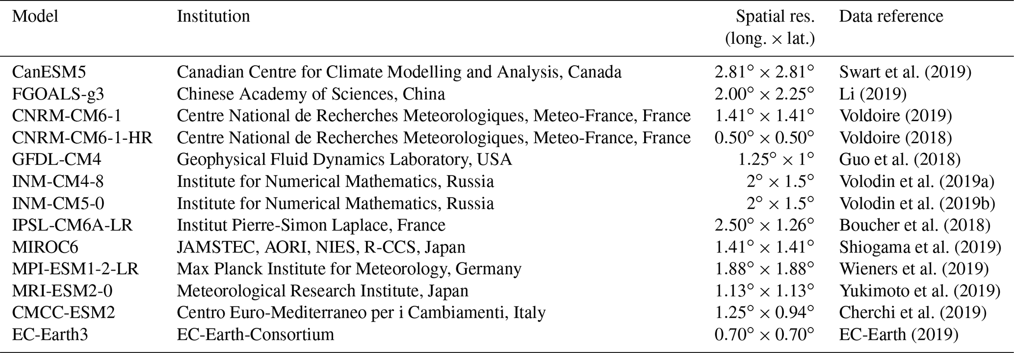
One ensemble of 13 global climate models (GCMs) following the CMIP6 protocol (Eyring et al., 2016) is considered. This selection of models is listed in Table 1. To define compound wind and precipitation extremes, we use daily precipitation and wind speed maxima variables. For growing-period frost, mean and minimum temperature variables are used. For each variable, the historical period simulations (1871–2014) have been extracted and extended until 2100 using the shared socioeconomic pathways 585 (SSP-585) scenario (Riahi et al., 2017). Since the 13 selected simulations present different spatial resolutions, each climate simulation dataset has been regridded to a common spatial resolution of $\mathrm{0.5}{}^{\circ }\times \mathrm{0.5}{}^{\circ }$ using bilinear interpolation. Considering the climate models separately will allow us to assess inter-model variability in terms of ToE of CE probabilities, as well as the potentially different contributions of marginal and dependence properties to changes in probability of multivariate climate hazards. Also, by considering all climate models together using a pooling procedure, a multi-model ensemble estimate for ToE and contributions may be derived. Pooling the models together will allow us better to take into account the global uncertainty inherent in climate modelling and to reduce the influence of natural variability amongst individual ensemble members.

Swart et al. (2019)Li (2019)Voldoire (2019)Voldoire (2018)Guo et al. (2018)Volodin et al. (2019a)Volodin et al. (2019b)Boucher et al. (2018)Shiogama et al. (2019)Wieners et al. (2019)Yukimoto et al. (2019)Cherchi et al. (2019)EC-Earth (2019)

Table 1 List of CMIP6 simulations used in this study, their run, approximate horizontal resolution and references.

For compounding wind and precipitation extremes, we use the spatial mean of daily wind speed maxima and the spatial sum of daily precipitation time series during winter (December, January and February) over the region of Brittany, France ($[-\mathrm{5},-\mathrm{2}{}^{\circ }\mathrm{E}]\times [\mathrm{46.5},\mathrm{49}{}^{\circ }\mathrm{N}]$, see Fig. 1a), which corresponds to a domain with 21 continental grid cells in our regridded climate simulations. This coastal region is regularly impacted by mid-latitude extra-tropical storms causing significant damage to infrastructures (e.g. storm Xynthia in 2010). Analysing the evolution of probability of compound wind and precipitations extremes is therefore relevant for this region. To allow for a robust statistical modelling of compounding wind and precipitation extremes, we applied our methodology to bivariate points of high values by selecting wind and precipitation data concurrently exceeding selected high thresholds. Indeed, our methodology detailed later in Sect. 3 is based on the use of parametric models, and considering the complete bivariate distribution to fit marginals and copulas may not be appropriate as the representation of the extremes would be biased by the bulk of the bivariate distributions where most of the data are located (e.g. Bevacqua et al., 2019). More details on selection thresholds are provided in Sect. 4.

Figure 1 (a) Map of France with the regions of interest in boxes. Scatterplots of CNRM-CM6 (b) DJF compounding wind and precipitation in Brittany and (c) minimal temperature in April and GDD values by the end of March over central France for the 1871–2100 period. Parametric fitting for marginal and dependence over the 30-year sliding windows spanning the 1871–2100 period to bivariate points in orange. For compounding wind and precipitation, these points correspond to high values of wind and precipitation data belonging to $S_{\mathrm{90},\mathrm{90}}^{\mathrm{CNRM}\text{-}\mathrm{CM}\mathrm{6}}$, i.e. simultaneously exceeding the individual 90th percentiles of the 1871–1900 reference period. Bivariate exceedance probabilities are then computed for varying exceedance thresholds between the 5th and 95th percentile of wind speed and precipitation already belonging to $S_{\mathrm{90},\mathrm{90}}^{\mathrm{CNRM}\text{-}\mathrm{CM}\mathrm{6}}$ (for more details, see Sect. 4). The red area contains bivariate points exceeding the 80th percentiles of points already belonging to $S_{\mathrm{90},\mathrm{90}}^{\mathrm{CNRM}\text{-}\mathrm{CM}\mathrm{6}}$. For growing-period frost, exceedance thresholds of interest for minimal temperature and GDD index are fixed to values of 0 and 200 ^∘C.day, respectively.

For growing-period frost events, data are extracted over central France ($[-\mathrm{1},\mathrm{5}{}^{\circ }\mathrm{E}]\times [\mathrm{46},\mathrm{49}{}^{\circ }\mathrm{N}]$, see Fig. 1a), which corresponds to 78 continental grid cells. The region covers an important agriculture area of France, including grapevine and fruit crops with high production (Vautard et al., 2022). We focus on the spatial mean of daily minimum temperature (T) in April to define frost events occurring in early spring. To account for phenology and to characterise bud burst conditions by the end of March, the growing degree day (GDD) model (Bonhomme, 2000) is used. The GDD model consists in computing cumulative daily mean temperatures minus a “base temperature” from a starting date. For our study, a base temperature of 5 ^∘C is used and the starting date for computing GDD values for each year is chosen to be 1 January. In this study, our aim is not to focus on the phenology of specific plants but rather to provide a general overview of growing-period frost events. Generally, 5 ^∘C as base temperature is accepted for crops and grapevine (e.g. Skaugen and Tveito, 2004; Jiang et al., 2011; Ruosteenoja et al., 2016; Vautard et al., 2022). Bud burst occurs when the cumulative sum of degree-days up to 31 March is larger than some thresholds (Garcia de Cortazar-Atauri et al., 2009) which depend on species. For each year y, GDD values by the end of March are obtained via the formula

$$\mathrm{GDD}\left(y\right):=\sum _{i=y/\mathrm{01}/\mathrm{01}}^{i=y/\mathrm{03}/\mathrm{31}}max\left(\mathrm{MT}\right(i)-\mathrm{5},\mathrm{0}),$$

with MT the daily mean temperature. GDD values are computed for each grid cell and averaged spatially over the area of central France. We consider the threshold of 200 ^∘C.day to characterise bud burst conditions and illustrate our method. The choice of this threshold is consistent with existing studies analysing bud burst values of grapevine species (e.g. Garcia de Cortazar-Atauri et al., 2009; Vautard et al., 2022), and is useful for characterising early bud burst plants that could be impacted by frost events.

For illustrative purposes, Fig. 1a displays the topographic map of France with the region of Brittany and central France in boxes. The bivariate wind and precipitation data (Fig. 1b) and minimal temperature and GDD data (Fig. 1c) for the CNRM-CM6 model are also displayed.

3 Statistical method

Our aim is to design a statistical method to assess the ToE of CE probabilities, that is to detect from which period changes of probability are statistically significant relative to a baseline period. Probabilities of CEs can be computed with copulas. Copulas are functions that make it possible to describe the dependence structure between random variables separately from their marginal distributions, which greatly simplifies calculations involving multivariate distributions (Nelsen, 2006). Copulas have been widely applied in climate and geophysical science (e.g. Vrac et al., 2005; Salvadori et al., 2007; Schölzel and Friederichs, 2008; Serinaldi, 2014). In addition to enabling computations of multivariate hazard probabilities, the use of copulas in our study allows us to isolate and quantify the marginal and dependence contributions of the variables forming the CEs to the overall probability changes. In the following, we first recall the concept of ToE, and then present our methodology to assess the ToE of CE probabilities. Then, after some remarks on copula theory, the methodology to assess the contribution of marginal and dependence properties to changes of probabilities is presented. For ease of presentation, the methodology is explained for compounding wind and precipitation extremes but will be applied similarly for growing-period frost.

3.1 Time of emergence of climate hazards

The concept of time of emergence (ToE) has been developed to assess the significance of climate changes relative to background variability. Comparing changes of climate signal relative to natural variability is particularly relevant as human societies and ecosystems are inherently adapted to the local background level of variability, and major impacts arise most likely when changes emerge from it (e.g. Lobell and Burke, 2008). Different methodologies to assess ToE of climate signals have been used in the literature. For example, ToE can be assessed by estimating the climate change signal (S) and the variability (or noise, N) of the climate metric of interest (e.g.  Hawkins and Sutton, 2012; Maraun, 2013; Hawkins et al., 2020; Ossó et al., 2022). The ToE is then estimated by determining the first period for which the $S/N$ ratio permanently crosses a certain threshold (e.g. emergence of “unusual” ($S/N>\mathrm{1}$), “unfamiliar” ($S/N>\mathrm{2}$), or “unknown” ($S/N>\mathrm{3}$) climates; Frame et al., 2017). Methodologies for ToE based on statistical tests have also been developed, which estimate the first period for which the distribution of the climate metric is significantly and permanently different from a baseline period distribution (e.g. using Kolmogorov–Smirnov tests; Mahlstein et al., 2012; Gaetani et al., 2020; Pohl et al., 2020). To define the emergence of CE probabilities, we propose to assess probabilities in a 30-year window sliding over the period 1871–2100 and compare their values with respect to a baseline period's probability. In this study, we consider the reference period (1871–1900) as baseline to assess the emergence of hazard probabilities. While most of the studies choose a pre-industrial period as baseline to attribute emergence to anthropogenic greenhouse gas forcing (e.g. 1850–1900, Hawkins et al., 2020), other studies choose a more recent baseline period (e.g. 1951–1983, Ossó et al., 2022), which can provide relevant information for adaptation planning. We further discuss the choice of the reference period for emergence in Sect. 6. The ToE of hazard probabilities is then the time period when a significant change of probability occurs relative to the probability associated with the estimated natural variability and persists until the end of the century. To assess whether probabilities are significantly different from that of the background variability, we propose to compute the 68 % and 95 % confidence intervals of the baseline period's probability. It allows us to characterise the natural variability of our probability of interest. An emergence is detected if probability for the 30-year sliding windows permanently goes out of the baseline confidence intervals (i.e. out of the estimated natural variability). The ToE is then defined as the central year of the sliding window over which the probability starts to emerge. As probabilities are estimated using copula modelling (see later in Sect. 3.2), 68 % and 95 % confidence intervals of the baseline period's probabilities are computed by coupling the parameter uncertainties of both the fitted marginal distributions and the fitted copula. Considering both 68 % and 95 % confidence intervals allows us to evaluate, with different degrees of confidence, the changes of probability of compounding events from the estimated natural variability. Details on the procedure to compute confidence intervals are given in Appendix A.

3.2 Copula functions and exceedance probability

In this study, we use copula modelling to compute CE probabilities. We first consider two random variables X (e.g. maximum wind speed) and Y (e.g. precipitation) for an arbitrary period. We denote their marginal (i.e. univariate) probability density functions (pdfs) f_X(x) and f_Y(y) and cumulative marginal distribution functions (CDFs) $F_X\left(x\right)=\mathbb{P}(X\le x)$ and $F_Y\left(y\right)=\mathbb{P}(Y\le y)$. Sklar's theorem (Sklar, 1959) states that, H, the joint (i.e. bivariate) CDF can be written as:

$$\begin{array}{}\text{(1)}& H_{X,Y}(x,y)=\mathbb{P}(X\le x\cap Y\le y)=C\left(F_X\right(x),F_Y(y\left)\right),\end{array}$$

where C is a function called “copula”, corresponding to the joint distribution function of the uniformly distributed variables F_X(X) and F_Y(Y). Under the assumption that the marginal distributions F_X and F_Y are continuous, Sklar's theorem states that the copula C is unique. This decomposition of the multivariate distribution into marginal distributions and copula function allows us to model the dependence among contributing variables independently of their marginals. Therefore, using copulas makes it easy to isolate the effects of marginal and dependence properties on the probability of multivariate hazards.

Bivariate exceedance probability refers to the probability that both random variables exceed a certain value (“AND approach”; Salvadori et al., 2016) and can be calculated relatively easily using copulas. For example, for wind and precipitation CEs, it corresponds to probabilities of wind speed and precipitation jointly exceeding established thresholds. We denote p_m,d the bivariate exceedance probability computed with marginal (subscript m) and dependence (subscript d) properties of (X,Y). The probability $p_{\mathrm{m},\mathrm{d}}(t_X,t_Y)$ that both X and Y jointly exceed some predefined thresholds t_X and t_Y is given by (Yue and Rasmussen, 2002; Shiau, 2003)

$$\begin{array}{}\text{(2)}& \begin{array}{rl}{p}_{\mathrm{m},\mathrm{d}}(t_X,t_Y)& =\mathbb{P}(X\ge t_X\cap Y\ge t_Y)\\ & =\mathrm{1}-F_X\left(t_X\right)-F_Y\left(t_Y\right)\\ & +C\left(F_X\right(t_X),F_Y(t_Y\left)\right).\end{array}\end{array}$$

Marginal and copula distributions in Eq. (2) are estimated using parametric fitting procedures. More details on the fitting procedures for compound wind and precipitation extreme and growing-period frost events are given in Appendix B.

3.3 Change in probabilities: contribution of the marginal and dependence properties

Let us now consider the realisations (X_ref,Y_ref) and (X_fut,Y_fut) of the two random variables X and Y over the reference period (i.e. 1871–1900 in the following), and over another 30-year period (e.g. a future period such as 2071–2100). Using Eq. (2), the reference and future bivariate exceedance probability $p_{{\mathrm{m}}_{\mathrm{ref}},{\mathrm{d}}_{\mathrm{ref}}}(t_X,t_Y)$ and $p_{{\mathrm{m}}_{\mathrm{fut}},{\mathrm{d}}_{\mathrm{fut}}}(t_X,t_Y)$ for some predefined thresholds t_X and t_Y are given by

$$\begin{array}{}\text{(3)}& {\displaystyle }\begin{array}{rl}{p}_{{\mathrm{m}}_{\mathrm{ref}},{\mathrm{d}}_{\mathrm{ref}}}(t_X,t_Y)& =\mathrm{1}-F_{X_{\mathrm{ref}}}\left(t_X\right)-F_{Y_{\mathrm{ref}}}\left(t_Y\right)\\ & +C_{\mathrm{ref}}\left(F_{X_{\mathrm{ref}}}\right(t_X),F_{Y_{\mathrm{ref}}}(t_Y\left)\right),\end{array}\text{(4)}& {\displaystyle }\begin{array}{rl}{p}_{{\mathrm{m}}_{\mathrm{fut}},{\mathrm{d}}_{\mathrm{fut}}}(t_X,t_Y)& =\mathrm{1}-F_{X_{\mathrm{fut}}}\left(t_X\right)-F_{Y_{\mathrm{fut}}}\left(t_Y\right)\\ & +C_{\mathrm{fut}}\left(F_{X_{\mathrm{fut}}}\right(t_X),F_{Y_{\mathrm{fut}}}(t_Y\left)\right).\end{array}\end{array}$$

As modelled here with Eqs. (3) and (4), $p_{{\mathrm{m}}_{\mathrm{fut}},{\mathrm{d}}_{\mathrm{fut}}}$ and ${}_{{\mathrm{m}}_{\mathrm{fut}},{\mathrm{d}}_{\mathrm{fut}}}$ can differ due to

• changes in the marginal properties of X and Y, i.e. changes between $F_{X_{\mathrm{ref}}}$ and $F_{X_{\mathrm{fut}}}$, as well as between $F_{Y_{\mathrm{ref}}}$ and $F_{Y_{\mathrm{fut}}}$,

• and changes in the dependence structure (i.e. in the copulas) between X and Y, i.e. changes between C_ref and C_fut.

Then, do exceedance probability values change significantly between reference and future periods? And if so, how much of this change is due to changing marginal properties, and how much is due to changing dependence structure? Attributing probability changes to changes of marginal and dependence properties has already been introduced by Bevacqua et al. (2019) to analyse compound flooding from precipitation and storm surge in Europe. However, to our knowledge, assessing those changes relative to a reference natural variability in a ToE context has not been done yet. In order to isolate the effects of these potentially changing statistical properties, we propose to calculate two additional exceedance probability values. The first one is the probability $p_{{\mathrm{m}}_{\mathrm{fut}},{\mathrm{d}}_{\mathrm{ref}}}$, which assesses what the future probability would be if only the marginal properties change between the reference and future period (and thus keeping the dependence properties from the reference period). $p_{{\mathrm{m}}_{\mathrm{fut}},{\mathrm{d}}_{\mathrm{ref}}}$ is hence computed as

$$\begin{array}{}\text{(5)}& \begin{array}{rl}{p}_{{\mathrm{m}}_{\mathrm{fut}},{\mathrm{d}}_{\mathrm{ref}}}(t_X,t_Y)& =\mathrm{1}-F_{X_{\mathrm{fut}}}\left(t_X\right)-F_{Y_{\mathrm{fut}}}\left(t_Y\right)\\ & +C_{\mathrm{ref}}\left(F_{X_{\mathrm{fut}}}\right(t_X),F_{Y_{\mathrm{fut}}}(t_Y\left)\right).\end{array}\end{array}$$

Inversely, the second additional probability $p_{{\mathrm{m}}_{\mathrm{ref}},{\mathrm{d}}_{\mathrm{fut}}}$ is aimed at assessing what the future probability would be if only the dependence properties change between the reference and future period (keeping the marginal properties from the reference period), and is computed as

$$\begin{array}{}\text{(6)}& \begin{array}{rl}{p}_{{\mathrm{m}}_{\mathrm{ref}},{\mathrm{d}}_{\mathrm{fut}}}(t_X,t_Y)& =\mathrm{1}-F_{X_{\mathrm{ref}}}\left(t_X\right)-F_{Y_{\mathrm{ref}}}\left(t_Y\right)\\ & +C_{\mathrm{fut}}\left(F_{X_{\mathrm{ref}}}\right(t_X),F_{Y_{\mathrm{ref}}}(t_Y\left)\right).\end{array}\end{array}$$

Illustrations of these four probabilities for artificial bivariate distributions and changes between a reference and a future period are given in Fig. 2.

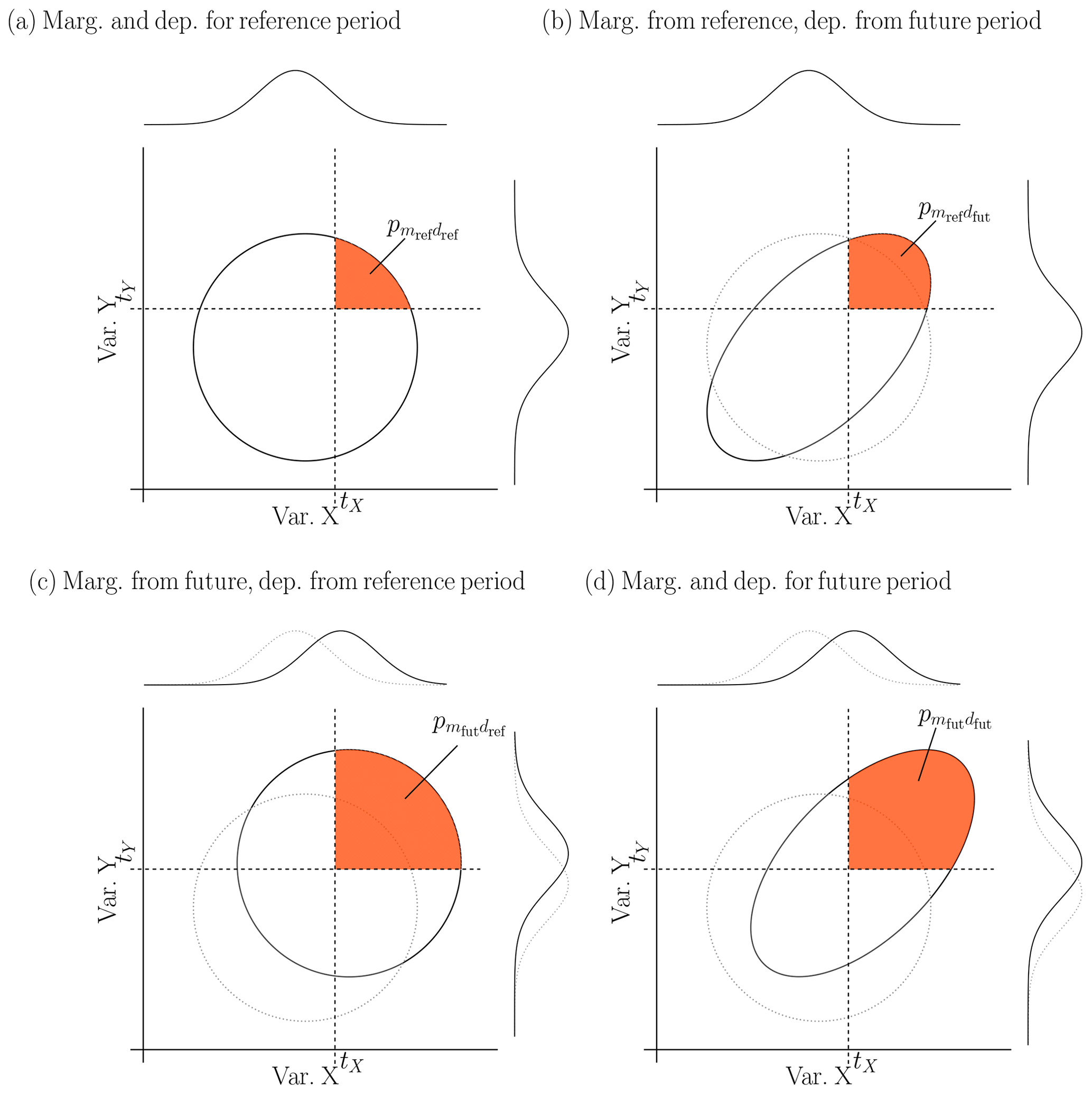
Figure 2 Illustration of the influence of marginal and dependence properties on bivariate exceedance probabilities for an artificial distribution of two contributing variables X and Y during (a) the reference period and (d) a future period with a shift in means and an increase in dependence between the variables. The distribution of the two contributing variables (b) with marginal properties from the reference period and dependence structure from the future period, and (c) with marginal properties from the future period and dependence structure from the reference period. Orange areas show bivariate exceedance probabilities for the thresholds (t_X,t_Y) of the two contributing variables.

To assess how much marginal and dependence properties contribute to exceedance probabilities change between reference and future period, we use the four probabilities derived above to decompose the overall probability change. We first define ΔP, the change of probability between the reference and future periods, as the difference between the two probabilities: $\mathrm{\Delta }P=p_{{\mathrm{m}}_{\mathrm{fut}},{\mathrm{d}}_{\mathrm{fut}}}-p_{{\mathrm{m}}_{\mathrm{ref}},{\mathrm{d}}_{\mathrm{ref}}}$. By computing $p_{{\mathrm{m}}_{\mathrm{fut}},{\mathrm{d}}_{\mathrm{ref}}}$ and $p_{{\mathrm{m}}_{\mathrm{ref}},{\mathrm{d}}_{\mathrm{fut}}}$, one can decompose the change of probability ΔP into a sum of three terms that can yield statistical interpretations:

$$\begin{array}{}\text{(7)}& \mathrm{\Delta }P=\mathrm{\Delta }M+\mathrm{\Delta }D+\mathrm{\Delta }I.\end{array}$$

The first term ΔM accounts for the difference of probability between the reference and future periods due to a change of marginal properties only and is hence called the “marginal” term:

$$\mathrm{\Delta }M=p_{{\mathrm{m}}_{\mathrm{fut}},{\mathrm{d}}_{\mathrm{ref}}}-p_{{\mathrm{m}}_{\mathrm{ref}},{\mathrm{d}}_{\mathrm{ref}}}$$

Similarly, the second term ΔD assesses the difference of probability between the reference and future periods due to a change of dependence properties only and is hence called the “dependence” term:

$$\mathrm{\Delta }D=p_{{\mathrm{m}}_{\mathrm{ref}},d_{\mathrm{fut}}}-p_{{\mathrm{m}}_{\mathrm{ref}},{\mathrm{d}}_{\mathrm{ref}}}$$

As simultaneous changes of marginal and dependence properties between the reference and future period can affect the exceedance probability in a highly non-linear fashion (as can be seen in Fig. 2), ΔP cannot be simply expressed as the sum of the differences ΔM and ΔD. Thus, a residual term ΔI, called the “interaction” term, is introduced to assess the part of the probability change that is due to the simultaneous change of marginal and dependence properties and that cannot be explained by the changes of these statistical properties separately:

$$\mathrm{\Delta }I=p_{{\mathrm{m}}_{\mathrm{fut}},{\mathrm{d}}_{\mathrm{fut}}}-p_{{\mathrm{m}}_{\mathrm{fut}},{\mathrm{d}}_{\mathrm{ref}}}-p_{{\mathrm{m}}_{\mathrm{ref}},{\mathrm{d}}_{\mathrm{fut}}}+p_{{\mathrm{m}}_{\mathrm{ref}},{\mathrm{d}}_{\mathrm{ref}}}.$$

The decomposition of ΔP into these three terms allows us to isolate the effects of the changes of marginal properties, the effects of the changes of dependence properties and the effects of the changes of interaction on the overall change of probability value ΔP. By taking advantage of this decomposition, we propose to quantify the contribution (in %) of the different terms ΔM, ΔD and ΔI to the change of probability ΔP. For example, the contribution of the changes of the marginal properties can be quantified as

$$\begin{array}{}\text{(8)}& {\mathrm{Contrib}}_{\mathrm{\Delta }M}={\displaystyle \frac{\mathrm{\Delta }M}{\mathrm{\Delta }P}}\times \mathrm{100},={\displaystyle \frac{p_{{\mathrm{m}}_{\mathrm{fut}},{\mathrm{d}}_{\mathrm{ref}}}-p_{{\mathrm{m}}_{\mathrm{ref}},{\mathrm{d}}_{\mathrm{ref}}}}{p_{{\mathrm{m}}_{\mathrm{fut}},{\mathrm{d}}_{\mathrm{fut}}}-p_{{\mathrm{m}}_{\mathrm{ref}},{\mathrm{d}}_{\mathrm{ref}}}}}\times \mathrm{100}.\end{array}$$

A value of 50 % for Contrib_ΔM would indicate that the change of marginal properties is responsible for 50 % of the global change of probability ΔP between the reference and future periods. The contributions of ΔD (or ΔI) can be calculated the same way by simply replacing ΔM in Eq. (8) by ΔD (or ΔI). The sum of the three contributions adds up to 100 %, by construction. Please note that, for illustration, changes of probability ΔP, ΔM and ΔD are here considered as differences of probabilities. One could also consider analysing other metrics such as relative differences (“r. diff”) by dividing each of the terms in Eq. (7) by $p_{{\mathrm{m}}_{\mathrm{ref}},{\mathrm{d}}_{\mathrm{ref}}}$:

$$\begin{array}{c}{\displaystyle }\mathrm{\Delta }{P}^{\mathrm{r}.\mathrm{diff}}={\displaystyle \frac{p_{{\mathrm{m}}_{\mathrm{fut}},{\mathrm{d}}_{\mathrm{fut}}}-p_{{\mathrm{m}}_{\mathrm{ref}},{\mathrm{d}}_{\mathrm{ref}}}}{p_{{\mathrm{m}}_{\mathrm{ref}},{\mathrm{d}}_{\mathrm{ref}}}}},\\ {\displaystyle }\mathrm{\Delta }{M}^{\mathrm{r}.\mathrm{diff}}={\displaystyle \frac{p_{{\mathrm{m}}_{\mathrm{fut}},{\mathrm{d}}_{\mathrm{ref}}}-p_{{\mathrm{m}}_{\mathrm{ref}},{\mathrm{d}}_{\mathrm{ref}}}}{p_{{\mathrm{m}}_{\mathrm{ref}},{\mathrm{d}}_{\mathrm{ref}}}}},\\ {\displaystyle }\mathrm{\Delta }{D}^{\mathrm{r}.\mathrm{diff}}={\displaystyle \frac{p_{{\mathrm{m}}_{\mathrm{ref}},{\mathrm{d}}_{\mathrm{fut}}}-p_{{\mathrm{m}}_{\mathrm{ref}},{\mathrm{d}}_{\mathrm{ref}}}}{p_{{\mathrm{m}}_{\mathrm{ref}},{\mathrm{d}}_{\mathrm{ref}}}}},\\ {\displaystyle }\mathrm{\Delta }{I}^{\mathrm{r}.\mathrm{diff}}={\displaystyle \frac{p_{{\mathrm{m}}_{\mathrm{fut}},{\mathrm{d}}_{\mathrm{fut}}}-p_{{\mathrm{m}}_{\mathrm{fut}},{\mathrm{d}}_{\mathrm{ref}}}-p_{{\mathrm{m}}_{\mathrm{ref}},{\mathrm{d}}_{\mathrm{fut}}}+p_{{\mathrm{m}}_{\mathrm{ref}},{\mathrm{d}}_{\mathrm{ref}}}}{p_{{\mathrm{m}}_{\mathrm{ref}},{\mathrm{d}}_{\mathrm{ref}}}}}.\end{array}$$

In addition, bivariate fraction of attributable risk (“FAR”, e.g. Stott et al., 2016; Chiang et al., 2021; Zscheischler and Lehner, 2021) can also be computed by dividing each of the terms by $p_{{\mathrm{m}}_{\mathrm{fut}},{\mathrm{d}}_{\mathrm{fut}}}$:

$$\begin{array}{c}{\displaystyle }\mathrm{\Delta }{P}^{\mathrm{FAR}}={\displaystyle \frac{p_{{\mathrm{m}}_{\mathrm{fut}},{\mathrm{d}}_{\mathrm{fut}}}-p_{{\mathrm{m}}_{\mathrm{ref}},{\mathrm{d}}_{\mathrm{ref}}}}{p_{{\mathrm{m}}_{\mathrm{fut}},{\mathrm{d}}_{\mathrm{fut}}}}},\\ {\displaystyle }\mathrm{\Delta }{M}^{\mathrm{FAR}}={\displaystyle \frac{p_{{\mathrm{m}}_{\mathrm{fut}},{\mathrm{d}}_{\mathrm{ref}}}-p_{{\mathrm{m}}_{\mathrm{ref}},{\mathrm{d}}_{\mathrm{ref}}}}{p_{{\mathrm{m}}_{\mathrm{fut}},{\mathrm{d}}_{\mathrm{fut}}}}},\\ {\displaystyle }\mathrm{\Delta }{D}^{\mathrm{FAR}}={\displaystyle \frac{p_{{\mathrm{m}}_{\mathrm{ref}},{\mathrm{d}}_{\mathrm{fut}}}-p_{{\mathrm{m}}_{\mathrm{ref}},{\mathrm{d}}_{\mathrm{ref}}}}{p_{{\mathrm{m}}_{\mathrm{fut}},{\mathrm{d}}_{\mathrm{fut}}}}},\\ {\displaystyle }\mathrm{\Delta }{I}^{\mathrm{FAR}}={\displaystyle \frac{p_{{\mathrm{m}}_{\mathrm{fut}},{\mathrm{d}}_{\mathrm{fut}}}-p_{{\mathrm{m}}_{\mathrm{fut}},{\mathrm{d}}_{\mathrm{ref}}}-p_{{\mathrm{m}}_{\mathrm{ref}},{\mathrm{d}}_{\mathrm{fut}}}+p_{{\mathrm{m}}_{\mathrm{ref}},{\mathrm{d}}_{\mathrm{ref}}}}{p_{{\mathrm{m}}_{\mathrm{fut}},{\mathrm{d}}_{\mathrm{fut}}}}}.\end{array}$$

However, by construction, results for contributions, either for relative differences or bivariate FAR, would be identical to those obtained for differences.

The methodology described above to assess ToE of CE probabilities and marginal and dependence contributions to these changes is applied to the 13 CMIP6 models by considering successively all 30-year sliding windows spanning the period 1871–2100. The methodology is applied to each climate model individually (“Indiv-Ensemble” version). In particular for contributions and ToE, multi-model median estimates are derived to summarise the information given by all the models. The Indiv-Ensemble version makes it possible to analyse the modelling of hazards separately and to assess the uncertainty in ToE arising from the inter-model differences. We also applied the methodology in the “Full-Ensemble” version, which consists of pooling the contributing variables of the 13 climate models together to derive unique ToE estimates and contribution values accounting for the global uncertainty in climate modelling. However, the details of the “Full-Ensemble” version and its results are not discussed in the main article but are given in Sects. S1–S5 in the Supplement. A summary of the successive steps of our methodology for the Indiv-Ensemble version is provided in the form of a flowchart in Fig. 3.

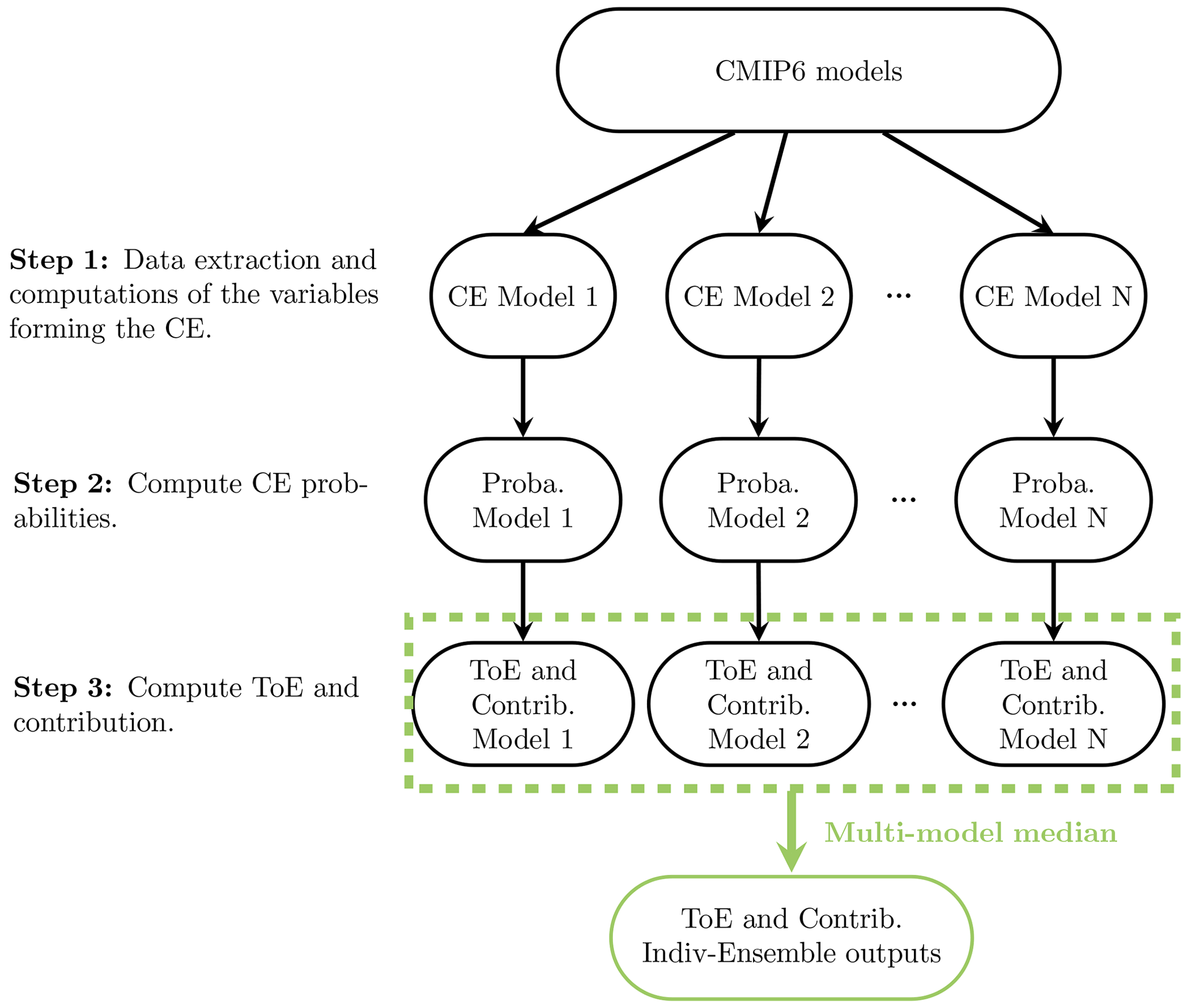
Figure 3 Flowchart for the computations of time of emergence and contributions for the Indiv-Ensemble version.

4 Results for compounding wind and precipitation extremes

In this section, results are presented for compound wind and precipitation extremes during winter in Brittany. Please note that, for this section as well as for the rest of the study, the period 1871–1900 is considered as the baseline period for natural variability to evaluate ToE and contributions. To focus on wind and precipitation extremes, we applied our methodology to points of high values. For each model, we selected points where, concurrently, wind and precipitation values exceed the individual 90th percentiles (denoted x_sel and y_sel, respectively) of the 1871–1900 reference period. In the following, we denote $S_{\mathrm{90},\mathrm{90}}^i$ the ensemble of the selected points of high values for a model i. For illustrative purpose, the ensemble $S_{\mathrm{90},\mathrm{90}}^{\mathrm{CNRM}\text{-}\mathrm{CM}\mathrm{6}}$ for the CNRM-CM6 model is shown in orange in Fig 1b. We first illustrate our method with a single climate model (CNRM-CM6). Then, results obtained for the Indiv-Ensemble version are presented.

4.1 Results for an individual model and a single exceedance threshold: CNRM-CM6

To illustrate our methodology, we first explain the results obtained for compound wind and precipitation extremes and a single bivariate exceedance threshold before extending the results to several bivariate thresholds. We evaluate the probabilities of exceeding the 80th percentiles of the bivariate points belonging to $S_{\mathrm{90},\mathrm{90}}^{\mathrm{CNRM}\text{-}\mathrm{CM}\mathrm{6}}$. The 80th percentiles for wind and precipitation correspond to $x_{\mathrm{80}|\mathrm{sel}}\approx \mathrm{17.8}$ m s⁻¹ and $y_{\mathrm{80}|\mathrm{sel}}\approx \mathrm{338}$ mm d⁻¹, respectively.

Before computing any probability, Fig. 4 gives an initial overview of the fitted bivariate distributions of compound wind and precipitation extremes in our study. It displays the evolution of the bivariate distributions over a selection of sliding windows due to changing marginal and dependence properties (“Marg.-dep.”, Fig. 4a), changing marginal properties only (“Marg.”, Fig. 4b) and changing dependence only (“Dep.”, Fig. 4c). Plotting these bivariate distributions already indicates the changes in probability of wind and precipitation extremes, and the potential influences of marginal and dependence properties on these changes. Indeed, at first sight in Fig. 4a, the area of bivariate distributions where wind speed and precipitation jointly exceed x_80|sel and y_80|sel appears to increase for future periods, suggesting that such bivariate events are more likely to occur according to CNRM-CM6 projections. But is this change of probability significant? And is this change due to changes in marginal properties or in dependence properties or in both? By keeping the dependence properties of the reference period and considering changing marginal properties only (Fig. 4b), an increase of exceedance probability seems to be observed, although less pronounced. Similar observations can be made by keeping the marginal properties of the reference period and considering changing dependence properties only (Fig. 4c). If both marginal and dependence changes seem to have an importance in the increase of probability, it is important to quantify how much these statistical properties contribute to the change of the overall probability as well as their respective influence on the ToE of probabilities of compounding wind and precipitation extremes.

Figure 4 Change of winter (December to February) bivariate wind and precipitation extremes distributions in Brittany based on CNRM-CM6 simulations due to (a) future marginal and dependence changes (“Marg.-dep.”), (b) future marginal changes while keeping dependence properties of the reference period (“Marg.”) and (c) dependence changes while keeping marginal properties of the reference period (“Dep.”). For the bivariate distributions, contour lines encompassing 90 % of all data points are shown. A selection of six 30-year sliding windows are presented using a colour gradient from light (1871–1900) to dark (2071–2100). The dashed red lines characterise the bivariate exceedance thresholds defined here as the 80th quantile of each variable.

Time series of exceedance probabilities over all sliding windows for the bivariate threshold (x_80|sel, y_80|sel) are presented in Fig. 5 by considering changes of marginal and dependence properties together (Fig. 5a) and separately (Fig. 5b and c). The 68 % and 95 % confidence intervals resulting from marginal and copula uncertainties are also displayed for each probability. All three time series present an increase with time, which is consistent with the visual analysis made in Fig. 4. Probability increase is less pronounced when future marginal (Fig. 5b) and future dependence properties (Fig. 5c) are considered separately. It illustrates that the effects of these changing statistical properties combine on exceedance probabilities. Yet, all three probability signals permanently go out of the reference natural variability confidence intervals, suggesting that an emergence of probability occurs: for probabilities computed with future marginal and dependence properties (Fig. 5a), the ToE is detected in 2009 (1994–2023) and 2072 (2057–2086) for 68 % and 95 % confidence levels, respectively. Concerning probabilities influenced by future marginal changes and future dependence changes separately (Fig. 5b and c), probability signals emerge later at the 68 % confidence level, in 2073 (2058–2087) and 2063 (2048–2077), respectively. If contributions of the statistical properties to ToE in itself are not computed here, one can get an idea of the importance of the statistical properties in ToE: at the 68 % confidence level, ignoring the dependence change would induce a ToE $\mathrm{2073}-\mathrm{2009}=\mathrm{64}$ years later. Similarly, ignoring marginal changes would induce a ToE $\mathrm{2063}-\mathrm{2009}=\mathrm{54}$ years later. It thus indicates that both marginal and dependence properties have a non-negligible effect on ToE.

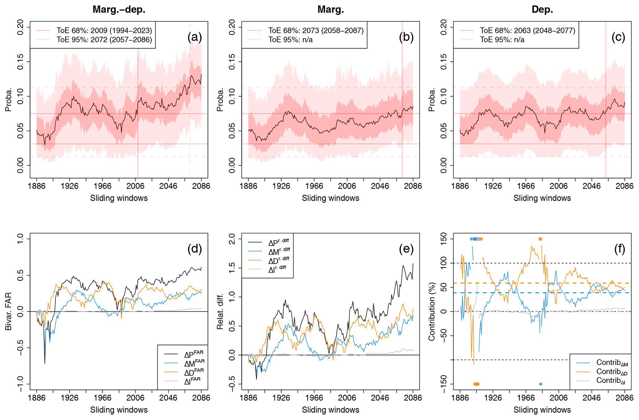
Figure 5 (a–c) Probability changes and time of emergence of compound wind and precipitation extremes $\left(\mathbb{P}\right(X>x_{\mathrm{80}|\mathrm{sel}}\cap Y>y_{\mathrm{80}|\mathrm{sel}}\mathrm{\mid }(X,Y)\in S_{\mathrm{90},\mathrm{90}}^{\mathrm{CNRM}\text{-}\mathrm{CM}\mathrm{6}}\left)\right)$ based on CNRM-CM6 simulations due to changes of (a) both marginal and dependence properties, (b) marginal properties only, and (c) dependence properties only. The shaded bands indicate 68 % and 95 % confidence intervals of the probabilities. Evolution of (d) the bivariate fraction of attributable risk (FAR), (e) relative difference of probabilities with respect to the reference period (1871–1900) and (f) contribution of the marginal, dependence and interaction terms to probability values. Median contributions computed over all sliding windows are displayed with dashed lines. Asterisks indicate values lying outside the plotted range. Not applicable (n/a) is indicated when no time of emergence is detected.

The evolution of the bivariate FAR ΔP^FAR with respect to the reference period over sliding windows, as well as its decomposition in terms of “marginal” (ΔM^FAR), “dependence” (ΔD^FAR) and “interaction” (ΔI^FAR) terms, is displayed in Fig. 5d. As explained in Sect. 3, for each sliding window, the sum of ΔM^FAR, ΔD^FAR and ΔI^FAR is by construction equal to ΔP^FAR. The decomposition highlights that the influences of the marginal and of the dependence properties on bivariate FAR can vary with time. Also, the combination of individual effects of marginal and dependence changes on the overall probability changes is again illustrated: for example, by 2100, considering both future marginal and dependence changes leads to a value of FAR ΔP^FAR twice as high as those of ΔM^FAR and ΔD^FAR, respectively. Concerning the interaction term, its associated bivariate FAR is negligible, highlighting that most of the changes can be explained by the changing marginal and dependence properties separately. Results for relative differences are displayed in Fig. 5e, and the same conclusions can be drawn. Figure 5f shows the evolution of the contributions from the marginal, dependence and interaction terms to probability values over sliding windows. By computing the median of contributions over all sliding windows, we can see that both changes in the marginal and in the dependence properties contribute greatly to probability changes (≈50 %) in the CNRM-CM6 simulations, with a slightly more important contribution from dependence properties (dashed lines in Fig. 5f). One may note a symmetry between the contribution values of the marginal and the dependence terms over sliding windows. This can be explained by the way contribution values are computed. Indeed, as the sum of the three contributions adds up to 100 %, by construction, and the fact that the contribution from the interaction term is close to 0, contribution values of the marginal and the dependence terms covary symmetrically around 50 %.

4.2 Results for CNRM-CM6 and several exceedance thresholds

The results for ToE and contributions have so far been presented for the probability of events exceeding the 80th percentiles of selected points belonging to $S_{\mathrm{90},\mathrm{90}}^{\mathrm{CNRM}\text{-}\mathrm{CM}\mathrm{6}}$. In order to have a broader analysis of exceedance probabilities of compound wind and precipitation extremes, we repeat the methodology for all pairs of exceedance thresholds between the 5th and 95th percentiles (with steps of 5 percentiles) of selected points belonging to $S_{\mathrm{90},\mathrm{90}}^{\mathrm{CNRM}\text{-}\mathrm{CM}\mathrm{6}}$. Figure 6 displays the results obtained for the CNRM-CM6 ToE at the 68 % confidence level, by considering marginal and dependence changes (Fig. 6a), marginal changes only (Fig. 6b) and dependence changes only (Fig. 6c). Moreover, for each bivariate exceedance threshold, median contributions (over all sliding windows) of marginal (Fig. 6d), dependence (Fig. 6e) and interaction terms (Fig. 6f) are displayed. Results for ToE obtained at the 95 % confidence level are displayed in Fig. S2 and differences of ToE are displayed in Fig. S3. When varying the exceedance thresholds, different ToE results are obtained, depending on whether marginal and dependence changes are considered (Fig. 6a–c). ToE is found for most of the exceedance thresholds when considering both marginal and dependence changes (Fig. 6a) or marginal changes only (Fig. 6b). It is, however, not the case for dependence changes only (Fig. 6c), for which only specific pairs of exceedance thresholds can find ToE. Interestingly, these pairs correspond to very high compound wind and precipitation extremes. This indicates that dependence change plays an important role for the probability of such high extreme events. The importance of dependence properties can also be assessed visually by comparing Figs. 6a and b. Indeed, for approximately the same pairs of exceedance thresholds as those already identified in Fig. 6c, earlier ToEs are obtained when considering both marginal and dependence changes (Fig. 6a) than when considering only marginal changes (Fig. 6b). Concerning the median contributions over all sliding windows of the marginal (Fig. 6d), dependence (Fig. 6e) and interactions terms (Fig. 6f), results vary according to the exceedance thresholds considered. Whereas for a large proportion of the exceedance thresholds, changes in marginal properties contribute strongly to probability changes (Fig. 6d), changes in dependence properties contribute predominantly to probability changes of very high wind and precipitation extremes (Fig. 6e). Regarding the “interaction” term, its contributions are close to 0, indicating little influence on the probability changes.

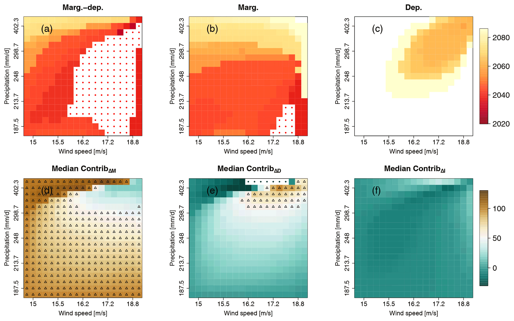
Figure 6 CNRM-CM6 (a–c) time of emergence (at 68 % confidence level) for compound wind and precipitation extremes due to changes of (a) both marginal and dependence properties, (b) marginal properties only, and (c) dependence properties only. White cells indicate that no time of emergence is detected, while white cells with red points indicate time of emergence values before 2020. (d–f) Matrices of median contributions of the (d) marginal, (e) dependence and (f) interaction terms. Results are presented for varying exceedance thresholds between the 5th and 95th percentile of compound wind and precipitation extremes data. Upper triangles show where the contribution is ≥50 %.

4.3 Results for the Indiv-Ensemble version and a single exceedance threshold

We now present the results obtained for ToE and contributions for the Indiv-Ensemble version for a single exceedance threshold. The methodology, previously illustrated with the CNRM-CM6 simulations, is now applied to each of the 13 models. Among the 13 models of the ensemble, only one model (INMCM-5.0) had more than 5 % of goodness-of-fit tests over all sliding windows, thus rejecting the hypothesis that the copula is a good fit, and hence was excluded from the analysis (see Appendix B for further details).

We first present the results obtained for probabilities of exceeding the 80th percentiles of selected points of high values of wind and precipitation for the 1871–1900 reference period. Figure 7 presents the results obtained. Probability time series obtained for the 12 models when considering changes of marginal and dependence properties(Fig. 7a), marginal properties (Fig. 7b) and dependence properties (Fig. 7c) are displayed, as well as ToE at the 68 % confidence level for the individual models and their multi-model median estimate. When considering future changes of both marginal and dependence properties (Fig. 7a), half of the models ($\mathrm{6}/\mathrm{12}$) detect a ToE at the 68 % confidence level. When found, a relatively important variability of ToE across climate models is obtained (varying between 2009 (1994–2023) and 2083 (2068–2097), Fig. 7a). These different results – i.e. either a ToE is detected or not, and the important variability of the year of emergence when found – indicate discrepancies in the statistical properties of compound wind and precipitation extremes between climate models. For marginal changes (Fig. 7b), seven models out of 12 detect a ToE, within a smaller range of values. It suggests a slightly better agreement of marginal changes for future periods between models when ToE is defined. Moreover, models that show emergence when considering marginal changes only are not necessarily those that show emergence when considering both future marginal and dependence changes. Indeed, two out of the seven models emerging with marginal changes are not those from the six emerging when marginal and dependence changes are taken into account (not shown). Hence, marginal changes alone are not always sufficient to make the probability signal emerge. Concerning dependence changes (Fig. 7c), two models out of 12 detect a ToE, indicating that dependence property changes for these two models influence greatly the exceedance probabilities by 2100. However, it also suggests that, for most of the models, the influence of the changes in dependence properties on exceedance probabilities is too small to make the probability signals go out of the reference confidence interval by 2100. These results on the stationarity of dependence structures complement those of Vrac et al. (2022b), where the ability of CMIP6 models to capture and represent significant changes in inter-variable dependencies is questioned. ToE results at the 95 % confidence level are displayed in Fig. S5 and are summarised using boxplots in Fig. S7.

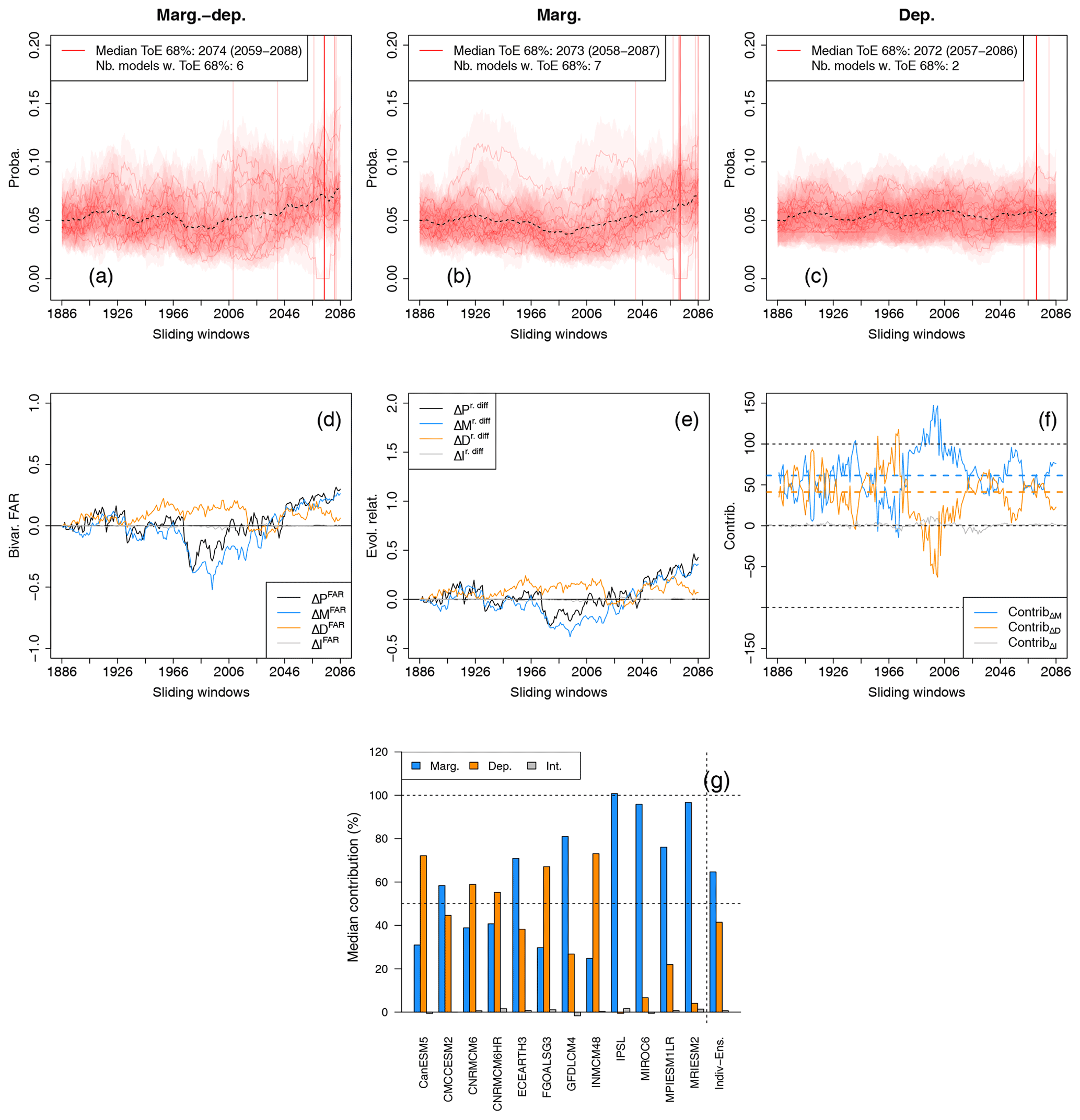
Figure 7 (a–c) Same as Fig. 5a–c but for the 12 individual CMIP6 models of the ensemble. Individual time of emergence is displayed when defined (vertical light red lines), as well as the corresponding median time of emergence (vertical red line). For information purposes, multi-model mean exceedance probability time series are also plotted (dotted black lines). (d–f) Same as Fig. 5d–f but for the Indiv-Ensemble version. Bivariate FAR, relative differences and contributions time series are computed by considering for each sliding window the median of the models' FAR, relative differences and contributions, respectively. (g) Median contribution of the marginal, dependence and interaction terms to overall probability changes for the 12 models and for the Indiv-Ensemble version.

The evolution of bivariate FAR, relative differences and contributions time series with respect to the reference period, as well as their decomposition in terms of marginal, dependence and interaction terms, is displayed in Fig. 7d–f, respectively. For reasons of brevity, the median of the 12 models' FAR, relative differences and contributions computed at each sliding window is plotted. The decomposition highlights again that the influences of the marginal and of the dependence properties on bivariate FAR, relative differences and contributions can vary with time.

Figure 7g displays the median contributions over all sliding windows for the 12 climate models separately, as well as for the Indiv-Ensemble version, i.e. by computing the median contribution of the models. Figure 7g shows that, depending on the model, different results are obtained for the contributions to probability changes. Indeed, while some models present balanced contributions, i.e. marginal and dependence terms contributing to ≈50 % each to probability changes (e.g. CMCC-ESM2, CNRM-CM6-1 and CNRM-CM6-1-HR), other models show very unbalanced contributions, with one statistical property mainly driving the probability changes. For example, the dependence term contributes predominantly (≥65 %) to probability changes for the models CanESM5, FGOALS-g3 and INM-CM-4-8, while the marginal term contributes the most for EC-Earth3, GFDL-CM4, IPSL-CM61-LR, MIROC6, MPI-ESM1-2-LR and MRI-ESM2-0. Results for the Indiv-Ensemble version indicate the contribution to probability changes of ≈60 % from changes in marginal properties and ≈40 % from changes in dependence properties. Concerning the interaction term, as obtained previously in Sect. 4.1, its contribution is close to 0 for each model individually.

4.4 Results for the Indiv-Ensemble version and several exceedance thresholds

As previously done in Sect. 4.2, we now compute ToE for all combinations of exceedance thresholds between the 5th and 95th percentiles in Fig. 8. Note that, here, exceedance thresholds are now expressed in terms of percentiles to enable a comparison of results. Figure 8a shows multi-model medians of ToE values induced by both marginal and dependence changes, i.e. results obtained for the Indiv-Ensemble version. A median value of ToE is obtained for any considered bivariate threshold, indicating that, for each exceedance threshold, at least one model presents an emergence. However, median ToE values show a variability depending on the bivariate exceedance thresholds. Note that the number of models presenting a ToE can also vary from one bivariate threshold to another. For each exceedance threshold, the number of models emerging at the 68 % confidence level, as well as interquartile values, are shown in Fig. S8. In particular, Fig. S8a indicates that all of the 12 models present a ToE for the probability of events exceeding very high precipitation and relatively low wind speed values (upper-left corner of the subplot). It suggests that all models agree on a change of the probability of occurrence of such events. This large consensus between models is not reached for events exceeding relatively low precipitation and very high wind speed values. Therefore, while all models simulate a significant increase of extreme precipitation events, this is not necessarily the case for extreme wind speed events. Results obtained for ToE induced by marginal properties only (Figs. 8b and S8b) are quite similar, although still indicating small differences with those obtained by considering marginal and dependence changes. Indeed, small differences of ToE can be observed, in particular for the upper-right area corresponding to very high wind speed and precipitation extremes. As observed in Sect. 4.1, this area corresponds to the area where changes in dependence properties lead to emerging exceedance probability from the reference period (Fig. 8c), suggesting their importance for the probability changes of such events. This result, however, should not be overstated, as only ≈2 models show dependence changes large enough to lead to the emergence of probability (Fig. S8c).

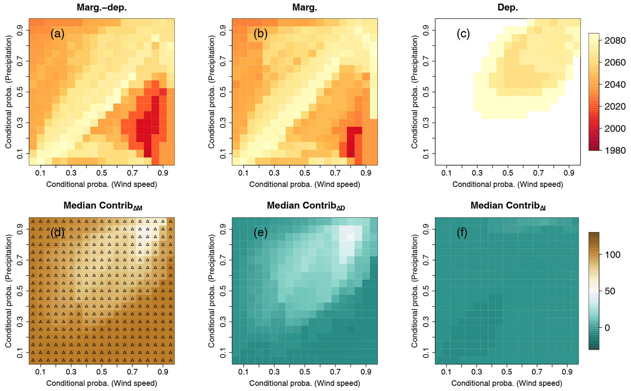
Figure 8 Time of emergence (at 68 % confidence level) matrices of compound wind and precipitation extremes for the Indiv-Ensemble version due to changes of (a) both marginal and dependence properties, (b) marginal properties only, and (c) dependence properties only. Results are displayed for varying exceedance thresholds between the 5th and 95th percentile of compound wind and precipitation extremes data. For (a–c), white indicates that no time of emergence is detected. Median contributions of (d) marginal, (e) dependence and (f) interaction terms. Upper triangles show where contribution is ≥50 %.

Median contribution of marginal, dependence and interactions terms is displayed in Fig. 8d–f, respectively. The results obtained previously concerning the importance of the marginal properties in probability changes are confirmed here: for all exceedance thresholds, changes in marginal properties contribute to more than 50 % of probability changes (Fig. 8d). Concerning the contribution of dependence changes (Fig. 8e), the median values obtained are less than 50 %, but specific pairs of exceedance thresholds highlight again the varying importance of dependence properties in exceedance probability changes: the median contribution of dependence properties is high for the probability changes of events exceeding high wind speed and high precipitation values. Concerning the interaction term (Fig. 8f), contribution values are equal to 0, highlighting again the negligible role of this term in probability changes. ToE results at the 95 % confidence level as well as the number of models emerging at the 95 % confidence level and interquartile values are shown in Figs. S11 and S12, respectively.

5 Results for growing-period frost events

We now apply our methodology to analyse a second type of CE: growing-period frost. Contrary to compound wind and precipitation extremes, for which we were interested in exceedance probabilities (i.e. both contributing variables exceedance thresholds), we are interested here in the probability of growing-period frost, i.e. the probability of having a GDD value exceeding a threshold of 200 (GDD ≥200) by the end of March – and hence characterising bud burst conditions – and having a frost in April, i.e. having T≤0. Hence, we applied our methodology described in Sect. 3 to bivariate points of GDD and minimal temperature data (one pair by year) by adapting Eq. (2) to compute the probabilities of interest. For example, for the probability of growing-period frost in the reference period, it is computed as follows (Yue and Rasmussen, 2002):

$$\begin{array}{}\text{(9)}& \begin{array}{rl}{p}_{\mathrm{m},\mathrm{d}}(\mathrm{0},\mathrm{200})& =\mathbb{P}(T\le \mathrm{0}\cap \mathrm{GDD}\ge \mathrm{200})\\ & =F_T\left(\mathrm{0}\right)-C\left(F_T\right(\mathrm{0}),F_{\mathrm{GDD}}(\mathrm{200}\left)\right).\end{array}\end{array}$$

Although the main results are presented for a threshold of 200 ^∘C.day, additional results for thresholds of 150 and 250 ^∘C.day are displayed in the Supplement to assess risks of growing-period frost for earlier and later bud burst plants.

5.1 Indiv-Ensemble results

We now present the results for the growing-period frost. As previously done, only one model (CMCC-ESM2) is excluded from the ensemble since it presents more than 5 % of goodness-of-fit tests, thus rejecting the hypothesis that fitted copulas are a good fit (see Appendix B for further details).

Figure 9 presents the results obtained for growing-period frost events. Results for 150 and 250 ^∘C.day GDD thresholds are presented in the Supplement in Figs. S15 and S16, respectively. By considering climate models separately, a ToE at the 68 % confidence level is detected for 11 out of 12 models when changes in marginal properties are taken into account (Fig. 9a and b). Although a large majority of models agree by simulating a significant change of growing-period frost probability with respect to the reference period, ToE values are quite scattered, indicating differences in simulations of growing-period frost events. By considering dependence changes only (Fig. 9c), none of the 12 models within the Indiv-Ensemble presents a ToE, indicating that the influence of dependence changes alone is not strong enough to modify growing-period frost probabilities. ToE values obtained for growing-period frost events are summarised in Fig. S17.

The evolution of bivariate FAR, relative differences and contributions time series for the Indiv-Ensemble version and their decomposition in terms of marginal, dependence and interaction terms are shown in Fig. 9d–f, respectively. Here the decomposition highlights that the influence of the marginal properties to change of probability is dominant along the whole time period for growing-period frost events, and that contributions of the dependence and interaction are rather limited. This is further confirmed in more detail by Fig. 9g, which displays the median contribution of the marginal, dependence and interaction terms to probability changes for each climate model individually and for the Indiv-Ensemble version. For the climate models individually, as well as for the Indiv-Ensemble version, the results are quite clear: marginal properties are the statistical properties contributing the most to probability changes of growing-period frost events.

Figure 9 Same as Fig. 7 but for growing-period frost events (GDD ≥200 ^∘C.day and minimal temperatures ≤0 ^∘C). For (a–c), not applicable (n/a) is indicated when no time of emergence is detected.

6 Summary and discussion

6.1 Summary

In this study, we have presented a new methodology to assess the ToE of compound hazards probabilities. Using a copula-based multivariate framework, we also propose to quantify the contributions of marginal and dependence properties to probability changes of hazards leading to CEs. The methodology has been applied to analyse two different climate hazards with potentially high impacts, using a 13-member multi-model ensemble (CMIP6): compounding wind and precipitation extremes in Brittany and growing-period frost events over central France. For each hazard, the methodology has been applied to individual climate models to derive ToE of probabilities and contributions of statistical properties of each model separately. It enables us to estimate the uncertainty in ToE values and contributions to multivariate hazards probability changes arising from inter-model difference.

Results for compounding wind and precipitation extremes over Brittany show that occurrence probabilities of such events are likely to increase and potentially emerge before the end of the 21st century. However, the reason for these increased probabilities can be different depending on climate models: while for some models, probability changes are mainly driven by marginal changes only, other models give a strong importance to both marginal properties and dependence properties. This results in having a mixed importance (∼65 % and 35 %) of both marginal and dependence properties that contribute to probability changes for the multi-model median. These results highlight the importance of carefully taking into consideration the dependence structure when studying the evolution of probabilities of compound wind and precipitation extremes.

Concerning growing-period frost events over central France, a large majority of models agree on the emergence of probabilities of such events. They also agree on the dominant contribution of marginal properties changes, while the contribution of dependence properties is mostly negligible.

By analysing two different case studies, our results highlight that the importance of marginal and dependence properties to probability changes can differ from one compound hazard to another, and from one climate model to another. It thus stresses the importance of considering both marginal and dependence properties carefully, as well as their inter-model variability, to analyse the future evolution of multivariate hazards leading to CEs.

6.2 Discussion and perspectives

In this study, the emergence of probabilities of multivariate hazards has been investigated with respect to the 30-year baseline period 1871–1900. This period can be considered as representative of the beginning of the industrial era (e.g. Hawkins et al., 2020) and can hence be of interest to assess if anthropogenic climate change has contributed to an emergence of probability of multivariate hazards. However, other baseline periods could have been chosen, such as more recent ones which would provide useful results for adaptation planning (e.g. Ossó et al., 2022). In practice, despite the changes in climate with respect to its natural variability, societies are (or should be) adapted to the present or recent climate. Hence, estimating the ToE relative to a more recent period, e.g. 1971–2000, would make it possible to provide results of more practical relevance for adaptation. Of course, depending on the chosen baseline period, the estimated natural variability that serves as reference for assessing changes would be different, and thus would affect the ToE results. As an illustration, Fig. S18 shows results from a quick sensitivity experiment for the ToE of probabilities of compounding wind and precipitation depending on the choice of the 30-year baseline period for the CNRM-CM6 model. It illustrates that results of emergence can vary strongly depending on the chosen baseline period. In addition to modifying the potential ToE, the choice of the baseline period can also influence the results of contributions from the changes in statistical properties (not shown), as these statistical changes are also assessed with respect to the baseline period. ToE and contribution results could also be modified by the choice of the length of the sliding windows. For example, considering a larger window length could attenuate the changes of statistical properties between the baseline period and the sliding windows, thus modifying the ToE results. Also, in a transient climate context, this results in mixing different climate conditions and, thus, different statistical properties. As an illustration, ToE and contribution results for the CNRM-CM6 simulations are presented in Figs. S19 and S20 by considering sliding windows of 40 years (baseline period: 1971–1910), 50 years (baseline period: 1971–1920) and 60 years (baseline period: 1971–1930) but are not commented on in the present study.

Moreover, in this study, the ToE of probability signals is defined as the year or time period for which the probability signal permanently exceeds a certain threshold (e.g. Hawkins and Sutton, 2012; Maraun, 2013; Hawkins et al., 2020). As the Earth's climate system is highly nonlinear and non-monotonic, detecting the emergence of a signal in this way can be limited depending on the climate signal under study. Analysing “periods of emergence” (PoE) instead of ToE may be more relevant to describe specific periods where probability signals emerge significantly – but temporarily – from reference natural variability. This notion of PoE would better highlight not only the non-linearities of the CE changes but also the differences in the evolution of probability between climate models, as was observed for growing-period frost events in Sect. 5. Indeed, in Fig. 9, while some climate models reach their highest growing-period frost probability for the late 21st century, other climate models present a decrease in probability to 0 for the end of the century after having reached maximum growing-period frost probability earlier. In other words, probabilities for future periods may differ, not permanently, but only temporarily from the estimated probability associated with natural variability. This could justify the development, the investigation and the use of the notion of temporary periods of emergence.

In addition, changes in marginal properties of the different variables and their contributions to probability changes have been assessed together, i.e. without separating the changes and contributions from wind and precipitation, nor those from GDD and minimum temperature. Thus, it does not allow us to quantify by how much changes in individual variables drive probability changes. Some studies already concluded on the importance of individual variables in the change of occurrence of multivariate hazards (e.g. Manning et al., 2018; Brunner et al., 2021; Calafat et al., 2022). Our methodology can, however, be easily adapted to quantify such information by keeping fixed marginal properties of only one contributing variable and by assessing probability changes. By doing this for the different variables in turn, the contribution of marginal changes to probability changes would be decomposed according to individual variable changes.

In this study, we demonstrated our conceptual framework using simulations from an ensemble of 13 GCMs. While using GCMs permitted us to illustrate our methodology and draw general conclusions when analysing changes of CE probabilities, the resolution of such climate models is often considered too coarse for a realistic representation of climate variables at a regional scale, such as for precipitation and wind (e.g.  IPCC, 2023). Consequently, the ToE results obtained in this study for Brittany and central France regions may not be accurate enough to be used for adaptation planning. Applying our methodology to analyse simulations from regional climate models (RCMs) that simulate physical processes at a higher spatial resolution would permit us to provide more relevant information on regional CEs that could be used to design realistic regional adaptation strategies. An appropriate future step could be, for example to apply the presented methodology to analyse CEs using simulations from RCMs forced by CMIP5 data (CORDEX) or CMIP6 data.

This study shows that both univariate and multivariate properties can be essential in determining CE properties. However, despite substantial improvements in climate modelling, climate simulations often remain biased compared to observations or reanalyses in terms of both univariate and multivariate properties (e.g. Cannon, 2018; Vrac, 2018; François et al., 2020). This could have major consequences on the ability of climate models to simulate CEs accurately (Zscheischler et al., 2019; Villalobos-Herrera et al., 2021; Vrac et al., 2022a; Ridder et al., 2021), and then on the resulting analyses involved in decision-making processes. A few multivariate bias correction methods, i.e. statistical methods that are able to adjust both univariate and multivariate properties of simulations with respect to reference datasets, have been recently developed (e.g. Cannon, 2018; Guo et al., 2019; Mehrotra and Sharma, 2019; Robin et al., 2019; Vrac and Thao, 2020; François et al., 2021). However, such MBC methods are designed to adjust the whole statistical distribution of climate simulations, and their abilities to increase the realism of specific parts of the statistical distribution (such as multivariate extremes) have never been tested, while this can be crucial for specific CEs. This is therefore an important perspective and the methodology developed in the present study could be a way to evaluate the consequences of MBC methods, e.g. in terms of ToE and contributions of marginal and dependence properties.

It should be noted that uncertainty in probabilities of multivariate hazards has been assessed by considering uncertainty in both statistical fitting procedures and model-to-model differences. However, uncertainty arising from internal climate variability, i.e. from the inherent chaotic nature of the climate system, has not been investigated. Assessing and analysing these uncertainties is, however, key to better characterising them and thus providing useful information for policy-makers (Raymond et al., 2022; Bevacqua et al., 2022). Future extensions of the framework presented herein could thus focus on using multimodel large-ensemble simulations to assess more robustly probabilities of hazards, the contributions of changes in statistical properties to their emergence, and their associated uncertainties resulting from both internal variability and structural model differences.

It is also important to note that the role of physical drivers of multivariate hazards has not been investigated in this study. Indeed, recent studies highlight the importance of large-scale climate modes (e.g. De Luca et al., 2020b; Singh et al., 2021b) and atmospheric circulation regimes (e.g. Faranda et al., 2020; Jézéquel et al., 2020; Vrac et al., 2022a) on compound and extreme events. Understanding the influence of physical drivers and their changes on the statistical features and probabilities of multivariate hazards is a key research area which has important implications for predicting their occurrence and characterising their impacts.

As mentioned in Sect. 1, the present methodology has been developed and applied in a ToE framework that is different from attribution. We have not considered factual and counterfactual worlds with different forcings to assess the effects of climate change on multivariate hazards probabilities. Adapting and applying our methodology in an attribution setting is thus an interesting perspective that would complement the existing multivariate event attribution framework recently developed (e.g. Kiriliouk and Naveau, 2020; Zscheischler and Lehner, 2021). In addition to attributing changes of CEs, our methodology would enable us to quantify the underlying contributions of the changes in marginal and dependence properties, hence better characterising the statistical features of climate change.

Appendix A: Procedure for estimation of confidence intervals

Confidence intervals of bivariate exceedance probabilities are estimated by combining the confidence intervals from the fitted parameters for both marginal distributions and copulas. For both marginal distributions and copulas, the fitted parameters and their 68 % (or. 95 %) confidence intervals are estimated using MLE (as described in Appendix B) and profile likelihood (e.g. Venzon and Moolgavkar, 1988; Hofert et al., 2012). Estimating the 68 % (or 95 %) confidence intervals for bivariate exceedance probabilities consists in (i) resampling uniformly and independently the fitted parameters of the two marginal distributions within their 68 % (or 95 %) profile likelihood confidence intervals, (ii) computing the bivariate exceedance probability using the resampled parameters for marginal distributions and the copula parameter estimated using MLE, (iii) repeating the two previous steps 100 times to construct a sampling distribution for the bivariate exceedance probability, (iv) searching which combinations of the resampled parameters lead to the 16 % and 84 % (or 2.5 % and 97.5 %) percentiles of the re-estimated bivariate exceedance probabilities, and (v) using the copula parameter uncertainty, estimating the 68 % (or 95 %) confidence intervals of the 16 % and 84 % (or 2.5 % and 97.5 %) percentiles of the bivariate exceedance probabilities. The lower and upper bounds of these two confidence intervals define the final confidence interval combining both marginal and copula parameters uncertainty.

Appendix B: Marginal and copula fitting

For the fitting of the marginal distributions, we considered the Akaike information criterion (AIC) to select the best families among Gaussian, generalised extreme value and generalised Pareto distributions. The marginal distributions of wind speed and precipitation beyond the selection thresholds were modelled by generalised Pareto distributions. For growing-period frost events, the marginal distributions of the GDD indices were modelled using Gaussian distributions. We modelled the negative of the minimal temperatures using GEV distributions and transformed back.

For fitting of the copulas, marginal distributions are transformed into uniform distribution using normalised ranks (e.g. Salvadori et al., 2011; Serinaldi, 2015; Bevacqua et al., 2019). This procedure is common for copula analysis as it allows us to perform appropriate goodness-of-fit tests (Genest et al., 2009). In this study, four Archimedean copulas (Clayton, Frank, Gumbel and Joe) are considered. These copulas have been widely used in hydrology and climate studies (e.g. Zscheischler and Seneviratne, 2017; Liu et al., 2018b; Tavakol et al., 2020) and allow the dependence structure to be modelled with a single parameter that determines the strength of the dependence. Moreover, the four Archimedean copulas differ in how they model dependence structures. For instance, the Gumbel and Joe copulas have upper tail dependence, which means that they are able to model correlated extremes. The Clayton copula has lower tail dependence and the Frank copula has no tail dependence. A complete overview of copula families, their related functions and the range of their parameters is offered by Sadegh et al. (2017). For each climate model and each sliding window, the best copula family is determined using the AIC. Copulas were fitted through maximum likelihood estimators (MLE) using the copula (Hofert et al., 2020) and VineCopula: (Schepsmeier et al., 2016) R-packages. Goodness of fit is tested based on White's information matrix equality (White, 1982; Huang and Prokhorov, 2014) implemented in the R package VineCopula (Schepsmeier et al., 2016). To evaluate exceedance probabilities, we select the copula family that has been the most selected along all the sliding windows and for which less than 5 % of the goodness-of-fit tests conclude on the rejection that the data fit well the considered copula distribution. Climate models for which more than 5 % of the goodness-of-fit tests conclude on a rejection are excluded.