Debris-flow surges of a very active alpine torrent: a field database

This paper presents a methodology to analyse debris flows focusing at the surge scale rather than the full scale of the debris-flow event, as well as its application to a French site. Providing bulk surge features like volume, peak discharge, front height, front velocity and Froude numbers allows for numerical and experimental debris-flow investigations to be designed with narrower physical ranges and thus for deeper scientific questions to be explored. We suggest a method to access such features at the surge scale that can be applied to a wide variety of monitoring stations. Requirements for monitoring stations for the methodology to be applicable include (i) flow height measurements, (ii) a cross-section assumption and (iii) a velocity estimation. Raw data from three monitoring stations on the Réal torrent (drainage area: 2 km², southeastern France) are used to illustrate an application to 34 surges measured from 2011 to 2020 at three monitoring stations. Volumes of debris-flow surges on the Réal torrent are typically sized at a few thousand cubic metres. The peak flow height of surges ranges from 1 to 2 m. The peak discharge range is around a few dozen cubic metres per second. Finally, we show that Froude numbers of such surges are near critical.

1 Introduction

The destructive nature of debris flows, as well as their sporadic behaviour, makes debris-flow measurements in the field difficult. Monitoring of debris flow was pioneered in the 1970s (e.g. in Japan, Suwa et al., 2011), and more monitoring stations have been developed in the past 20 years (Hürlimann et al., 2019), allowing for a wide range of debris-flow events in different torrent morphology to be observed. In their review, Hürlimann et al. (2019) show the various designs of the monitoring stations and their different objectives. Debris-flow monitoring is performed for various purposes including understanding debris-flow initiation (Bel, 2017) and increasing knowledge about the physics of the flows (Theule et al., 2018) and impact forces (Nagl et al., 2022).

However, despite years of efforts in monitoring these phenomena, few data on debris flows have been shared in open databases. The collective effort and interest in gathering such data would benefit from a structured method and definition of features of interest. One of the only available datasets was published by McArdell and Hirschberg (2020), who provided dates and bulk volumes of 75 debris-flow events measured on the Illgraben catchment in Switzerland; de Haas et al. (2022) published flow features (front height, velocity, flow rate, density, frontal shear stress), antecedent rainfall and channel bed elevation change for the Illgraben torrent for 13 events. Marchi et al. (2021) also provided an extensive study on the Moscardo catchment (Italian Alps), presenting data on triggering rainfall, flow velocity, peak discharge and volume of the monitored hydrographs. They made the complete dataset of debris-flow hydrographs and rainfall measurement for 26 events available in Marchi et al. (2020). In their paper, Comiti et al. (2014) published volumes, velocities and dates of two events measured on the Gadria catchment in Italy as an initial analysis, with the same intent as the present work, namely to formalize and centralize data on debris-flow processes. Other events that occurred on the same catchment were also described by Theule et al. (2018), Nagl et al. (2020) and Coviello et al. (2021). Guo et al. (2020) made available the velocity, flow depth, flow rate, flow width and duration of 23 surges for the Jiangjia Gully in China. Other data on debris-flow features can be found for the Chalk Cliff catchment in the United States (six events by McCoy et al., 2012) and one event for the Cancia catchment in Italy (Simoni et al., 2020). These few interesting initiatives pave the way for community-driven open databases; they were however extracted from raw data with various approaches making it difficult to pool them into a single consistent dataset.

Meanwhile, numerical methods improved tremendously in the recent years. Applications for debris-flow hazard mapping and the design of mitigation measures are increasingly attracting attention, allowing for evermore scientific questions to be answered (Jakob and Hungr, 2005). These methods are now mature enough to model parts of the complex phenomena observed in the field at multiple scales. However, the lack of comparable, relevant, openly available field data slows down the progress in performing more realistic debris-flow modelling. This leads to a disparity between field reality and numerical and laboratory experiments. There is, for instance, a habit of exploring very large ranges of Froude numbers in numerical studies of impact forces, typically 1–8 (e.g. among others Albaba et al., 2015; Ceccato et al., 2018; Ng et al., 2020). Performing such extensive parameter studies is a careful approach that ensures covering the poorly known variability of nature. However, it creates huge needs regarding experimental effort, computational power and time. These efforts are a high price to pay as they mean that more complicated scientific questions are not explored due to a lack of resources. In addition, in both experimental and numerical simulations, Froude numbers used are usually high, namely typically > 2–4 (e.g. Ng et al., 2020; Chen et al., 2020; Goodwin and Choi, 2022). Meanwhile, various regimes of impacts and flow behaviour emerge depending on the Froude number (Faug et al., 2012), but the transition seems to occur for lower Froude values; typically they are near critical (Laigle and Labbe, 2017). Whether it makes sense to study each regime highlighted in laboratory experiments for field application should be decided in light of field measurements. Thus, a database would ensure using features that are more representative of field reality, saving time to focus on deeper scientific questions.

Now that monitoring stations have been installed for a reasonable period of time, raw data processing is possible in order to build a common and open database on flow characteristics of debris-flow surges. Such a database would aim to give access to the scientific community for values of typical flow features such as volume, maximal flow height, peak discharge and Froude numbers of real debris flows. A methodology for debris-flow surge data processing is described in the present paper regarding focusing on the surge scale rather than a full-scale debris-flow event (several fronts and surges with intermediate diluted flows). Representing accurately one debris-flow surge is already a great challenge for modellers to face, both numerically and experimentally, and being able to have the physical feature of a surge will help in achieving this challenge.

The end goal of this paper is to define a common methodology that is sufficiently simple to apply so as to make it widely usable at any automated debris-flow monitoring station. Using it will then permit gathering characteristics of debris-flow surges in a homogeneous, easy-to-access database. Surge identification, velocity computation and volume determination methods are more thoroughly described in this paper. The methodology we used to process monitoring data is first presented in this paper. Its application to the three monitoring stations of the Réal catchment in southeastern France is then explained. The results describe the values of the surge parameters and show synthetically the interest of having several stations in the same channel in a catchment. However, the methodology is not restricted to such monitoring scenarios. The range features of surges are first put into perspective with the literature. Potential relationships and the evolution of surge features are then investigated, and conclusive remarks are drawn.

2 Material and methods

2.1 Methodology to compute the surge characteristics

2.1.1 Concept of the event analysis

Each monitoring station has different types of sensors and different strategies to measure flow characteristics (Hürlimann et al., 2019). To apply the methodology, the following measurements are required (Fig. 1):

• flow height measurements with a representative frequency sufficient to accurately describe the flow front rise on the hydrograph;

• a known cross-section where the flow is measured or an assumption about the relationship between flow height and the wetted area (to reduce calculation errors, it is necessary to have a precise estimation of the wetted area before, during and after a surge);

• a way to directly access the mean velocity of the surge, typically by estimating the travel time between a pair of sensors (potentially different types) at a sensible distance from one another or, more accurately but rarely available, by direct velocity measurement (e.g. image processing or large-scale particle image velocimetry; see Theule et al., 2018).

These measurements must be done at sufficiently close locations to reasonably assume that the measured flow height is associated with the measured surge velocity. Between two sensors, there should be no major change in flow path, channel width and slope so as to ensure that the geomorphological processes are consistent along the interdistance.

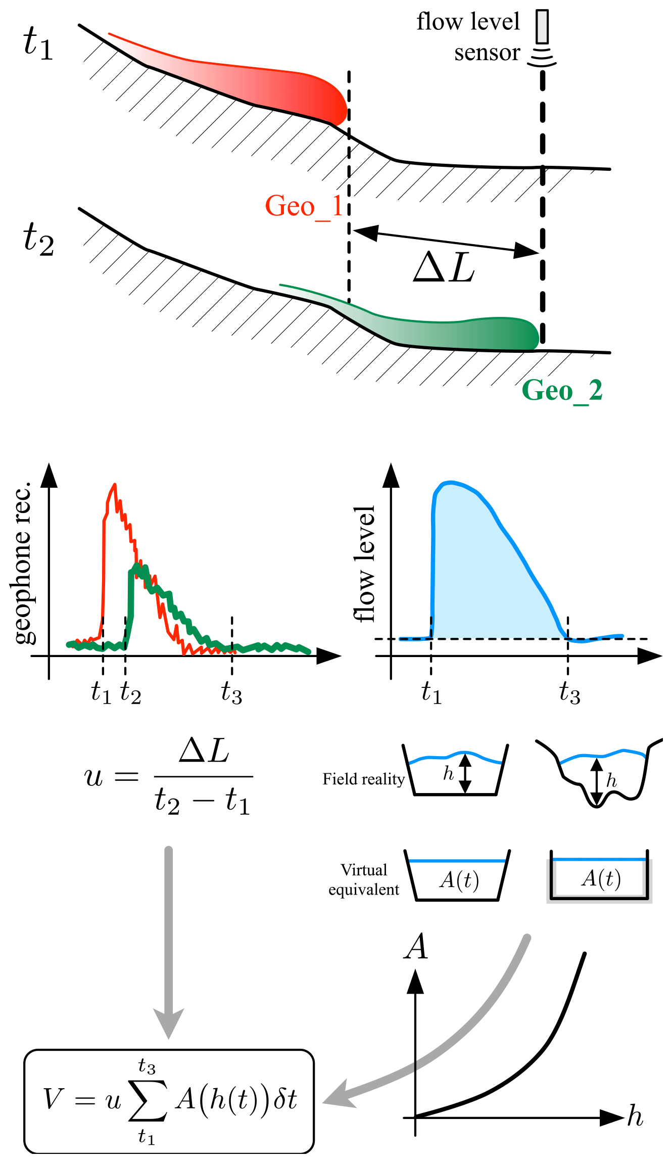
Figure 1 Synthetic overview of the method: a pair of sensors are used to estimate the time travel Δt between known locations, and an assumption about the cross-section shape along with the flow depth sensor is used to compute the wetted area A(t) and the associated surge parameters: discharge Q(t), volume V and Froude number Fr. The Geo_X labels represent sensors.

The key parameters describing the surges are then computed using the following time series:

$$\begin{array}{}\text{(1)}& {\displaystyle }Q\left(t\right)=u\cdot A\left(t\right),\text{(2)}& {\displaystyle }V=\sum Q\left(t\right)\cdot \mathit{\delta }t,\text{(3)}& {\displaystyle }\mathit{Fr}={\displaystyle \frac{u}{\sqrt{g\cdot h_{max}}}},\end{array}$$

where Q is the debris-flow discharge [m³ s⁻¹], t is the time [s], u is the mean surge velocity [m s⁻¹], A is the wetted section [m²], V is the surge volume [m³], $\mathit{\delta }t=\frac{\mathrm{1}}{f}$ is the time sampling interval [s], Fr is the Froude number [–], g is the gravitational acceleration [m s⁻²] and h_max is the maximum value of the flow depth [m].

2.1.2 Surge identification

A debris flow is generally composed of one or several surges, with potentially intermediate flows that are more diluted (called “diluted runoff” hereafter) (Hungr, 2005). The categories with the highest complexity, destructive power and interest in debris flows are most probably the surges and their fronts. As a consequence, the database aims at gathering measurements focusing on the surge fronts and their main body, rather than the full scale of the debris-flow event including several surges (e.g. as provided in McArdell and Hirschberg, 2020). In addition, it is arguable that diluted runoff has a lower sediment concentration and contributes much less significantly to the bulk event volume than the main, mature debris-flow surges. As a matter of fact, the applicability of Eqs. (1) and (2) relies on an assumption of high solid concentration (Hungr, 2005), constant throughout the surge. Focusing on data processing at the surge scale goes hand in hand with the intention for this database to be used to explore scientific questions on the surge front behaviour. This approach is different from other initiatives in the literature where the full scale of the event was considered.

Clearly defining the surges is thus a prerequisite to the data processing as the volume of the surge is integrated over the surge duration (Eq. 2), not the full event duration. If several surges in a single event are identified, each surge is taken separately as a data point in the database.

The most basic identification of the surges is performed on the flow height time series by identifying surges in the flow hydrograph. Doing so without cross control based on other information is however doubtful in catchments where diluted runoff and debris floods are frequent and intense. With experience, when available, images of the front can be used to define this separation. Geophone data proved to enable more reliable and data-driven criteria because they capture the solid transport intensity (Fontaine et al., 2017; Chmiel et al., 2022). Arattano et al. (2014) showed that the amplitude method for geophone signals allows for accurately detecting the passage of a debris-flow surge while allowing for lighter data acquisition. Other methods, such as the impulse method, have shown accurate results for debris-flow warning (Abancó et al., 2012). Bel (2017) showed that when mature debris flows travel at the levels of the geophones, this amplitude of the seismic activity is high and does not drop to zero. Immature debris-flow surge can also trigger an instantaneously high geophone signal but differs from mature debris flow because the signal frequently drops to zero during the event. This is why the criterion of determination between debris flows and immature debris flows cannot only be based on instantaneously high geophone signals. The existence of a prolonged period of consistently high seismic activity (with a high geophone signal) is chosen to differentiate debris-flow events from immature debris flows and debris floods. Diluted runoff is also easily differentiated from the surge using this method.

In Fig. 2, the concept of the identification is described. The onset of a surge is detected by both a sharp increase in flow height and a sharp increase in the amplitude of the geophone signal, followed by a consistently non-zero seismic activity. The end of a surge is determined either by seismic activity dropping to zero or by the onset of a second surge that can clearly be separated from the first one. Indeed, at the end of the first surge of the figure, a drop in seismic activity is clearly observed and a second sharp increase announces a second surge. On the other hand, the second surge displays two peaks in the flow level, but as the seismic activity stays consistently high, those two peaks are considered part of one single surge.

Figure 2 Conceptual graph explaining the surge identification approach: t₁ marks the onset of the first surge, with a sharp increase in energy in the geophone aligned with the flow sensor and sharp increase in directly measured flow height; t₂ marks the end of the first surge and the start of the second surge, with geophone activity decreasing before a sharp increase due to a second surge; t₃ marks the end of the second surge, with seismic activity being negligible even though the flow height is still high – those are the diluted runoff flows; and t₄ marks the start of the third surge. Note that even though the second surge has two peaks on the flow height, it is seen as one surge due to continuous seismic activity.

2.1.3 Velocity calculation

In the proposed approach, as shown in Eq. (1), a single velocity value is considered for each surge. By doing so, the authors knowingly assume that the velocity is uniform within the surge. This is a crude simplification of the complex rheology of debris flows. The assumption is however required due to the lack of more precise data on most monitoring sites (see an exception in Nagl et al., 2020). This surge average velocity is a relevant proxy for the front velocity. Carefully defining the surge main body and consistently not including diluted runoff is a pivot point of this approach, as this approximation on the velocity is more relevant if the surge is only restricted to its front and main body (see Sect. 2.1.2).

The velocity is generally computed using the lag Δt between the signals of two sensors and the known interdistance ΔL between those sensors. The distance is taken as the average flow path between the sensors, i.e. the path of the main channel between the two sensors. Once the lag is determined, the velocity is computed as $u=\frac{\mathrm{\Delta }L}{\mathrm{\Delta }t}$. Accessing the value of this lag is done by comparing the two signals and their timescale characteristics. Choosing two sensors that are at a sensible distance one from another is important: choosing two sensors too close to each other will induce significant uncertainty in the lag measurement. Due to the direct comparison of signals, the approach assumes that the source of the signal is the same that was propagating between the two different locations; in other words, the same surge is detected at both locations. This approach thus also assumes that the surge does not significantly change between the two sensors (e.g. no massive deposition or erosion, no strong change in surge duration, no merging between surges). However, the travel distance should be sufficiently longer than the uncertainty in the lag so as to provide an accurate estimate. Two methods were used to estimate velocities: the cross-correlation of signals if they were good enough and a visual identification method otherwise. For more information, the detailed methodology is presented in the Supplement.

2.1.4 Wetted area

From raw data, the flow height and wetted area are determined at each time step. This requires assumptions about the channel bed level. Two examples will be presented in this section: assumptions that are reasonable on a check dam and assumptions about a natural cross-section.

On controlled cross-sections, e.g. on a check dam crest, it is assumed that there is neither erosion nor deposition. Consequently, the bed level and cross-section shape are assumed to be constant and known. The flow height and wetted area can then easily be estimated. This configuration is preferable. Practically this means $h_{\mathrm{effective}}=z_{\mathrm{measured}}-z_{\mathrm{dam}}$, where h_effective is the effective flow height [m], z_measured is the level of the free surface measured by the sensor [m] and z_dam is the check dam crest level [m]. The wetted-area shape can be more accurately described by taking into account its convex surface shape (regarding its cross-section) (see Jacquemart et al., 2017).

Erosion and deposition occurring during debris-flow events may change the channel geometry. Not only does this mean that $h_{\mathrm{effective}}\ne z_{\mathrm{measured}}-z_{\mathrm{bed}}$, where z_bed would be the bed level before the flow [m], but it also means the cross-section shape will change during the event. The erosion–deposition process has two consequences: uncertainty in the channel shape and uncertainty in the channel bed level at a given time during the surge.

Accounting for the variability in the channel is necessary (e.g. width, bed level, shape). Due to the debris-flow event, scouring or filling can occur both vertically and horizontally to the cross-section. For each station, assumptions about cross-section shape have to be made, and questions about variability in the channel have to be answered. For example, assumptions about cross-section shape and change must answer whether the channel can be scoured or filled in that section and whether there is a difference in the preferred channel between low and high flows. Assumptions have to be as precise as possible using the information about the channel at this point (e.g. local obstructions to the flow are known, non-erodible banks).

Bed level change throughout the surge is explored using different assumptions (Fig. 3 and as seen in Fig. 11). With z_low, min, the minimal bed level through the event, the following three assumptions are made, when relevant:

• The whole depth of the flow is sheared (effective ) until z_low, min during the whole surge (assumption max).

• The flow is not sheared in depth; this is less likely but allows for computing a minimal possible volume (assumption min).

• In the case of an erosion process, the bed level is assumed to follow a fitted logarithmic law following Kaitna and Hübl (2021) (assumption log).

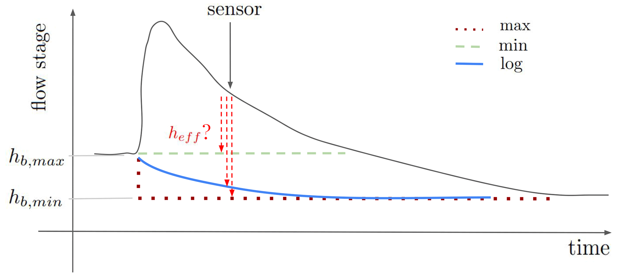
Figure 3 Assumptions about the bed level used to compute the efficient flow height in a natural cross-section: assumption max maximizes the effective (eff) flow height; assumption min minimizes the effective flow height.

2.2 Characteristics of the monitoring stations

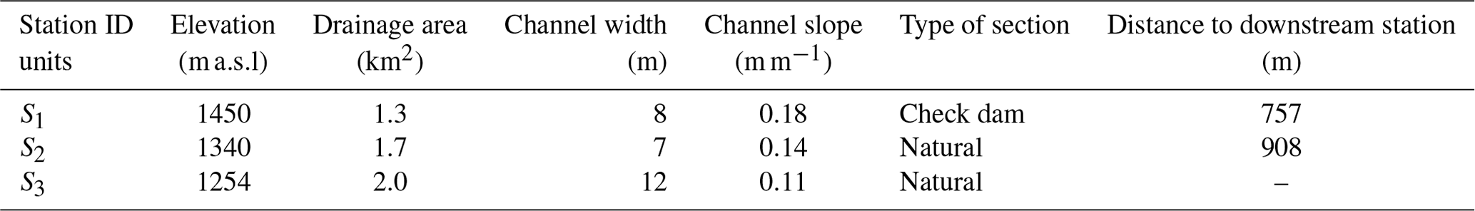
The Réal torrent, located in the south of France, has been instrumented since September 2010 (Navratil et al., 2011). Three monitoring stations are distributed along the channel. Figure 5 shows the station locations. The first one, station S₁, is located on a 20 m wide check dam as seen in Fig. 8a and is the most upstream. Stations S₂ and S₃ are located in the middle reach and at the outlet of the torrent and are both on natural cross-sections. In Table 1, a summary of the main physical features of the stations is shown (drawn from Bel et al., 2017). The purpose of the installation is to monitor the flow height, rainfall and seismic activity during sediment activity from the bed load to debris flow. A thorough study of the station can be found in Fontaine et al. (2017) and in Bel (2017). The methodology presented above has been applied to these three stations, and the results are presented further in this paper.

Table 1 Physical features of the three monitoring stations.

In essence, each station is equipped with (i) a tipping-bucket rain gauge with 0.201 mm resolution (Campbell), (ii) an ultrasonic or radar flow stage sensor (Paratronic), and (iii) a set of three vertical geophones (Geospace GS20DX0) each spaced out ≈100 m apart from each other upstream, midstream and downstream of the flow height sensors.

Images of the channel and flow proved to be useful to facilitate the interpretation of the signals (Piton et al., 2017). Two cameras have been added to stations S₁ and S₂ (Campbell CC640; replaced in 2018 by a Reconyx PC900 and Canon EOS1200D, respectively). Data are recorded using an environmental data logger (Campbell CR1000) powered by a solar panel and are stored in a compact flash module (Campbell CFM100).

In Fig. 4a, a complete set of measurements for one debris-flow event at station S₁ exemplifies the data analysis for one event. Out of these raw measurements, the best suited signals are chosen by the user, as seen in Fig. 4b:

• For flow height along the event, if multiple flow height signals are available, the most reliable one is chosen, i.e. the flow height sensor that does not present any artefact (e.g. unphysical values, very noisy signal). Consistently choosing the same sensor across all events when it does not have any malfunctions is preferable. Here, only one is available.

• For the surge identification, one geophone signal is chosen, associated with the flow height signal. The sensors best suited for surge identification are those aligned with flow height sensors (see Fig 5; e.g. geo_2).

• For velocity determination, two geophone signals are chosen for cross-correlation. They must have the clear appearance of the debris-flow behaviour, with the continuously non-zero geophone signal explained in Sect. 2.1.2, and be at a sensible distance one from each other (e.g. geo_1 and geo_2).

The selection is mainly based on a visual estimation of which sensor is the most appropriate. The influence of that choice remains marginal.

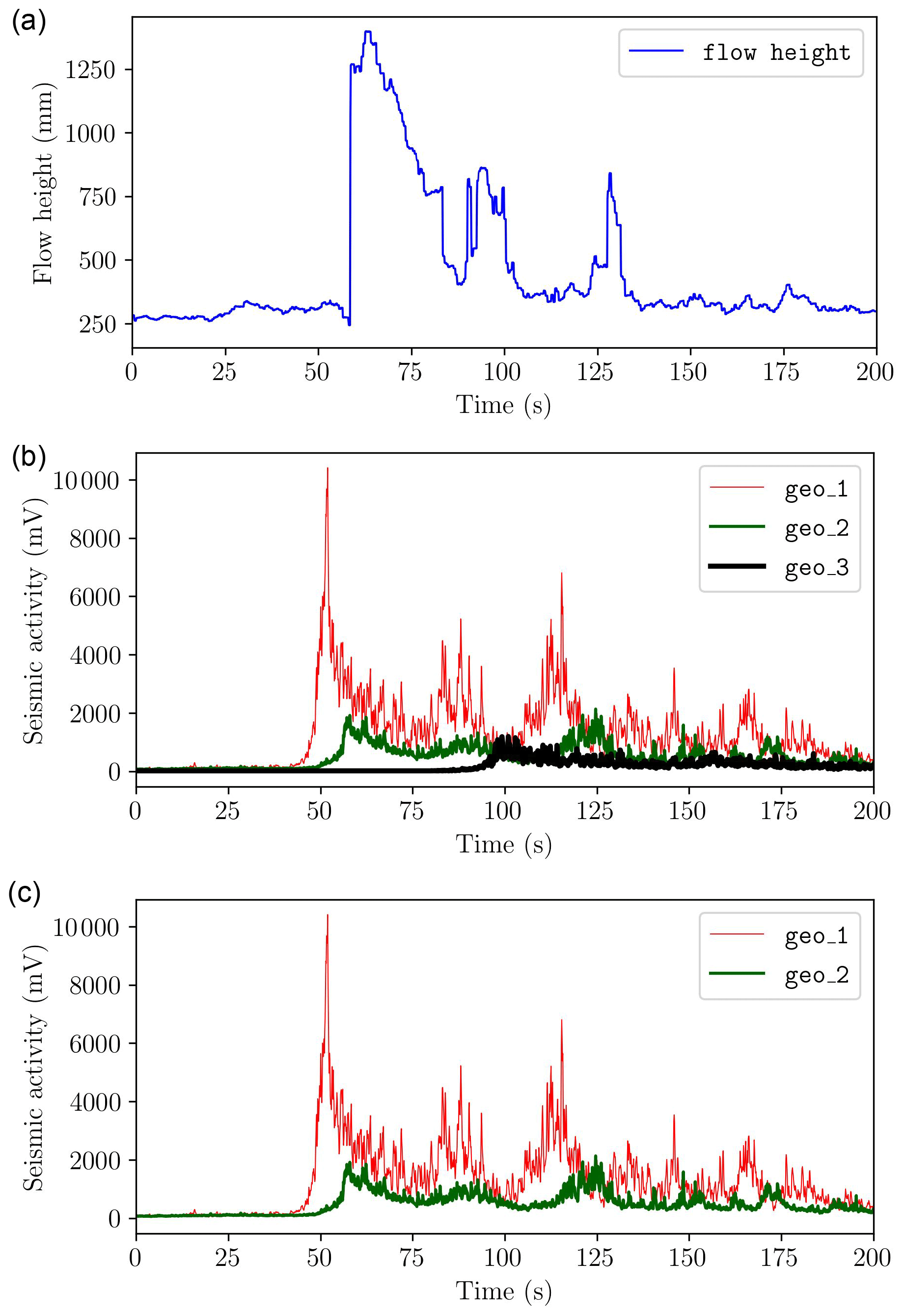
Figure 4 Overview of a recording of an event for station S₁; geo_X labels represent geophone signals: (a) flow height sensor, (b) full record of the geophone signal and (c) chosen signals.

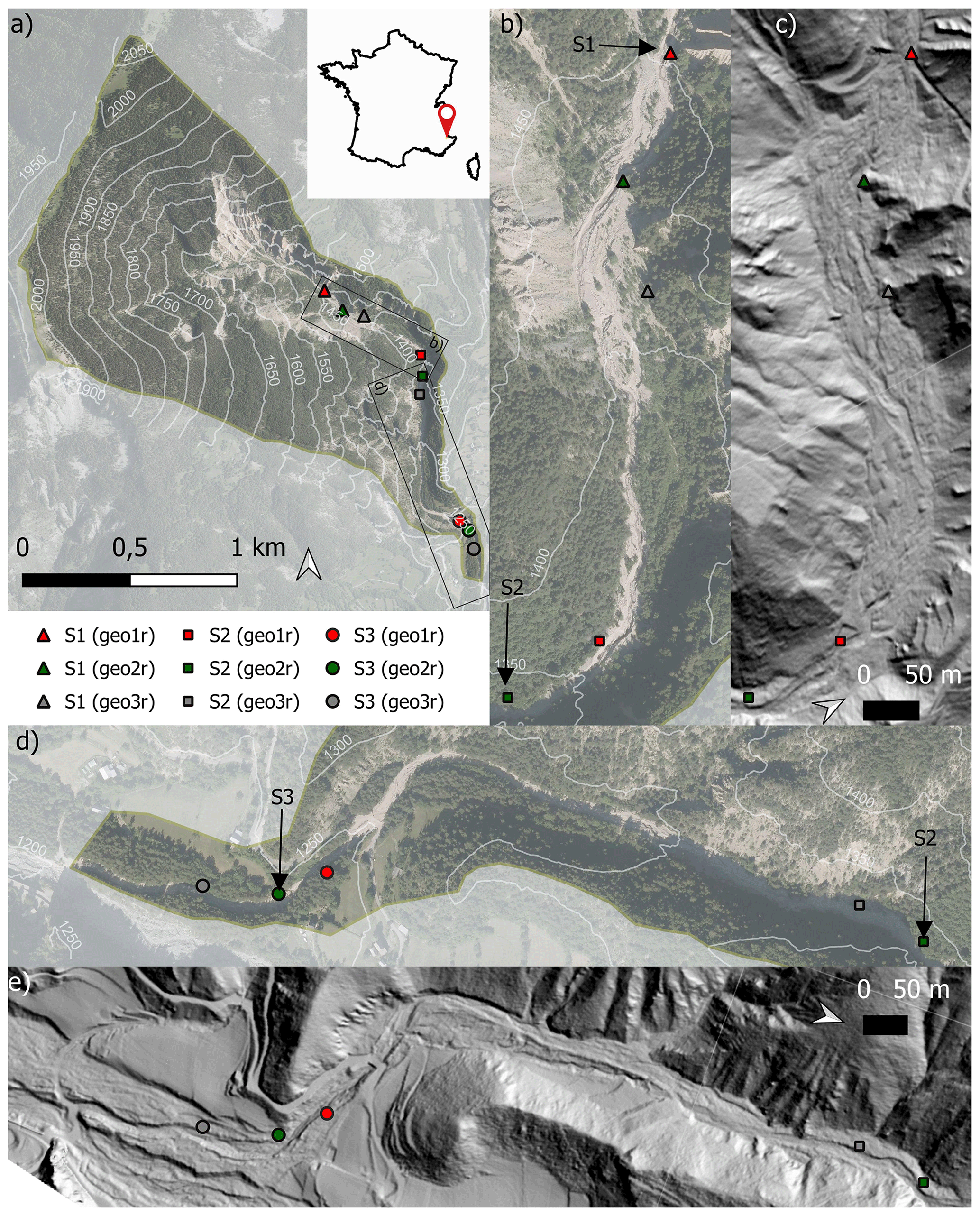
Figure 5 Overview of the installation on the Réal torrent. (a) Full location of the torrent and its stations. Drainage area is highlighted, as well as the three stations. Arrows show the position of the flow height sensor. The geo_XX labels denominate the geophones at each station (r or l signifies right or left bank). (b) Aerial photography of station S₁. (c) Digital elevation model (DEM) of station S₁. (d) Aerial photography of stations S₂ and S₃. (e) DEM of stations S₂ and S₃ (aerial pictures from BD ORTHO of the French geographical survey, IGN).

This leads to Fig. 4b with only the datasets used for the determination of the hydraulic values of interest. For each of these measurements, surges are identified and their features are computed. The user cross-controls the measurements and eventually goes for the visual method if the cross-correlation does not provide satisfying results (irrelevant value of velocity, low correlation coefficient or inconsistent velocity when compared to a first quick manual computation). The visual method consists in manually inputting the date of the onset of the surge on each geophone and considering the difference as the lag (see Fig. S3 in the Supplement). This visual method was used marginally, i.e. for one surge in our case, and was confirmed using image processing.

These sensors and post-processing allow for having the following for each event: (i) seismic activity at three different points around the station with a frequency of 5 or 10 Hz, (ii) rainfall data every 5 min (not used directly in this work), (iii) flow height with a frequency of 5 or 10 Hz, and (iv) imagery of the event (when possible) with a 0.2 or 1 Hz frequency.

Further in the paper, the value of the effective flow height is taken as the following:

• in the case of a controlled section, the mean value between the two assumptions for the section shape, as described in Bel (2017);

• in the case of erosion in a natural section, the logarithmic assumption;

• in the case of deposition in a natural section, the mean value between the min and max assumptions.

3 Results

3.1 Observed debris-flow surges

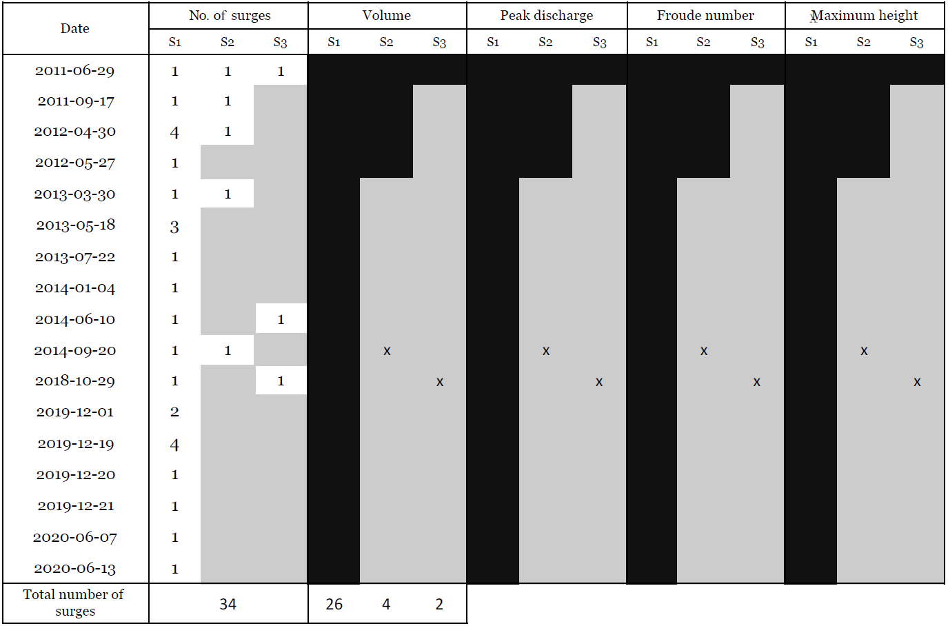
For the construction of the database, only significant events were considered to ensure the analysis of mature debris flows: a threshold of flow height above 1 m was selected for this catchment. This threshold is arbitrarily chosen from our experience on this particular catchments. Overall, 34 events were considered for the Réal station for the period 2011–2020. Table 2 shows when those events occurred, the number of surges passing at each station and the availability of the describing parameters. Over the 34 surges, most, i.e. 26, are recorded in upstream station S₁, while only four surges reached S₂ and only two reached S₃, the most downstream station. The lack of events in the period 2014–2018 is partially due to the natural variability in event sizes but also due to faulty sensors during that time period.

Table 2 Summary of the available data. Black cells correspond to available data. Grey cells are non-applicable. Crossed-out cells are events that were detected but for which the data were not retrieved due to faulty sensors. Please note that the date format in this table is year-month-day.

3.2 Distribution of surge parameters

One of the main interests in having an integrative dataset is to allow access to field ranges of hydraulic values of interest, such as Froude numbers and volumes of surges. In Fig. 6, different cumulative distribution functions (CDFs) of the datasets are presented. Froude numbers range from 0.25 to 1.6, showing the range of regimes found in debris flows in our site. Whether this is a site-specific feature or it can be shown at more sites that Froude numbers are typically critical would be a strong take-home message for the community.

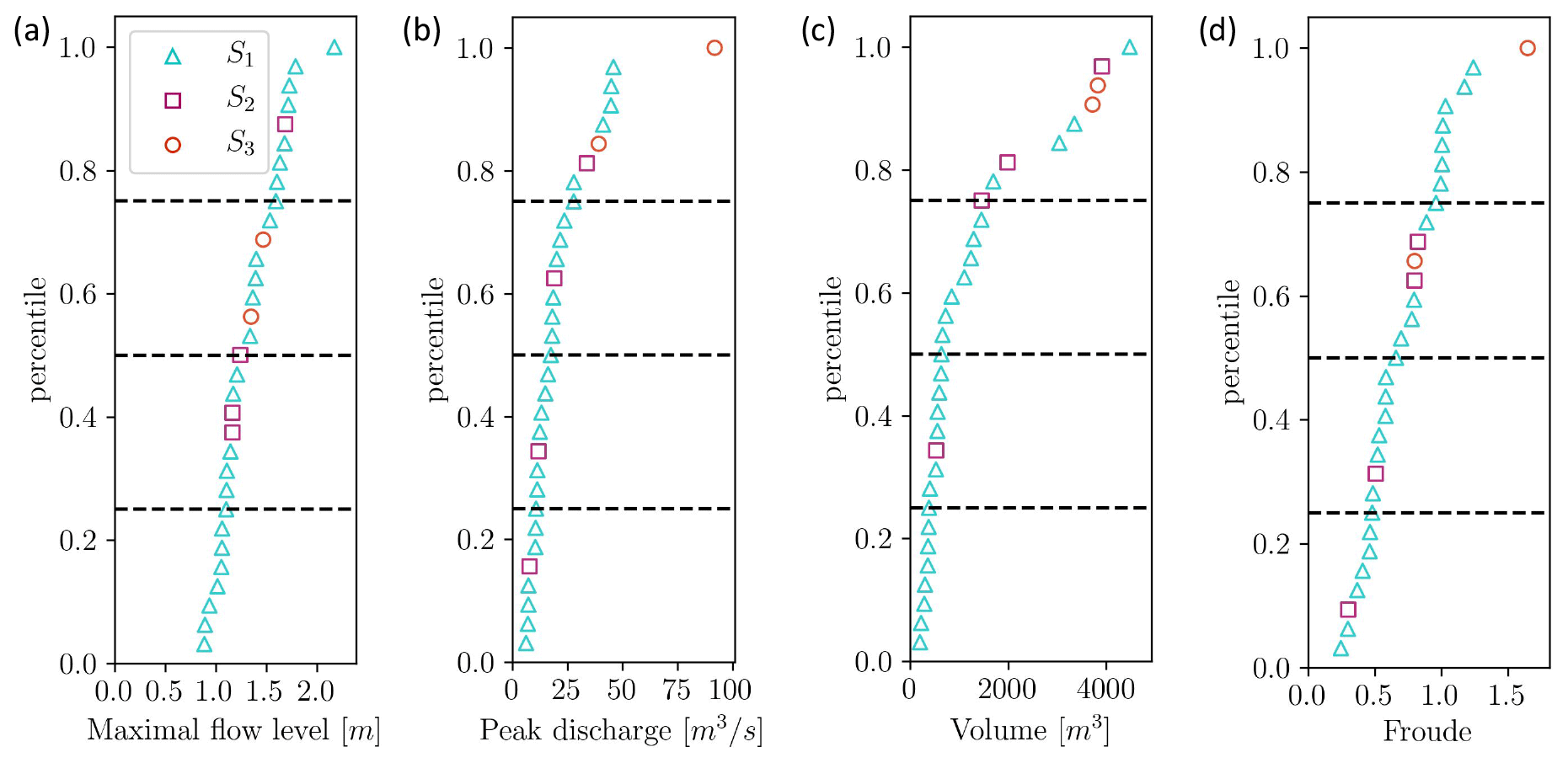
Figure 6 Cumulative density functions of hydraulic values of interest: (a) maximal flow level, (b) peak discharge, (c) volume and (d) Froude.

Surge volumes range from 200 to 4500 m³ (Fig. 6c; quantiles at 25 %, 50 % and 75 % of 390, 640 and 1460 m³, respectively). Surges are relatively small, typically from 1000 to 2000 m³ km⁻² (recall that this is a surge scale and an event may comprise several of them, e.g. 1–4 in our observations of Table 2, as well as some diluted runoff). Maximal flow height is most of the time lower than 2 m (Fig. 6a: quantiles at 25 %, 50 % and 75 % of 1.1, 1.25 and 1.6 m). The peak discharge ranges between 6.2 and 91.8 m³ s⁻¹ (Fig. 6b; quantiles at 25 %, 50 % and 75 % of 10.8, 17.5 and 27.9 m³ s⁻¹). The unit peak discharge is thus typically 0.775 to 7.65 m³ s⁻¹. Froude numbers range from 0.25 to 1.6 (Fig. 6d; quantiles at 25 %, 50 % and 75 % of 0.48, 0.65 and 0.95); i.e. they are typically near critical. The complete dataset is available in Table S1 in the Supplement.

Finally, relationships between these hydraulic values may be explored with a wider dataset and a more thorough description of each event. Figure 7 shows for instance the relationship between a few key variables (Froude numbers, volume of each surge normalized by the catchment area, front height and velocity). The surge volume was normalized by the catchment area not only to cross-compare measurements performed at different stations but also to help transfer these results to other catchments.

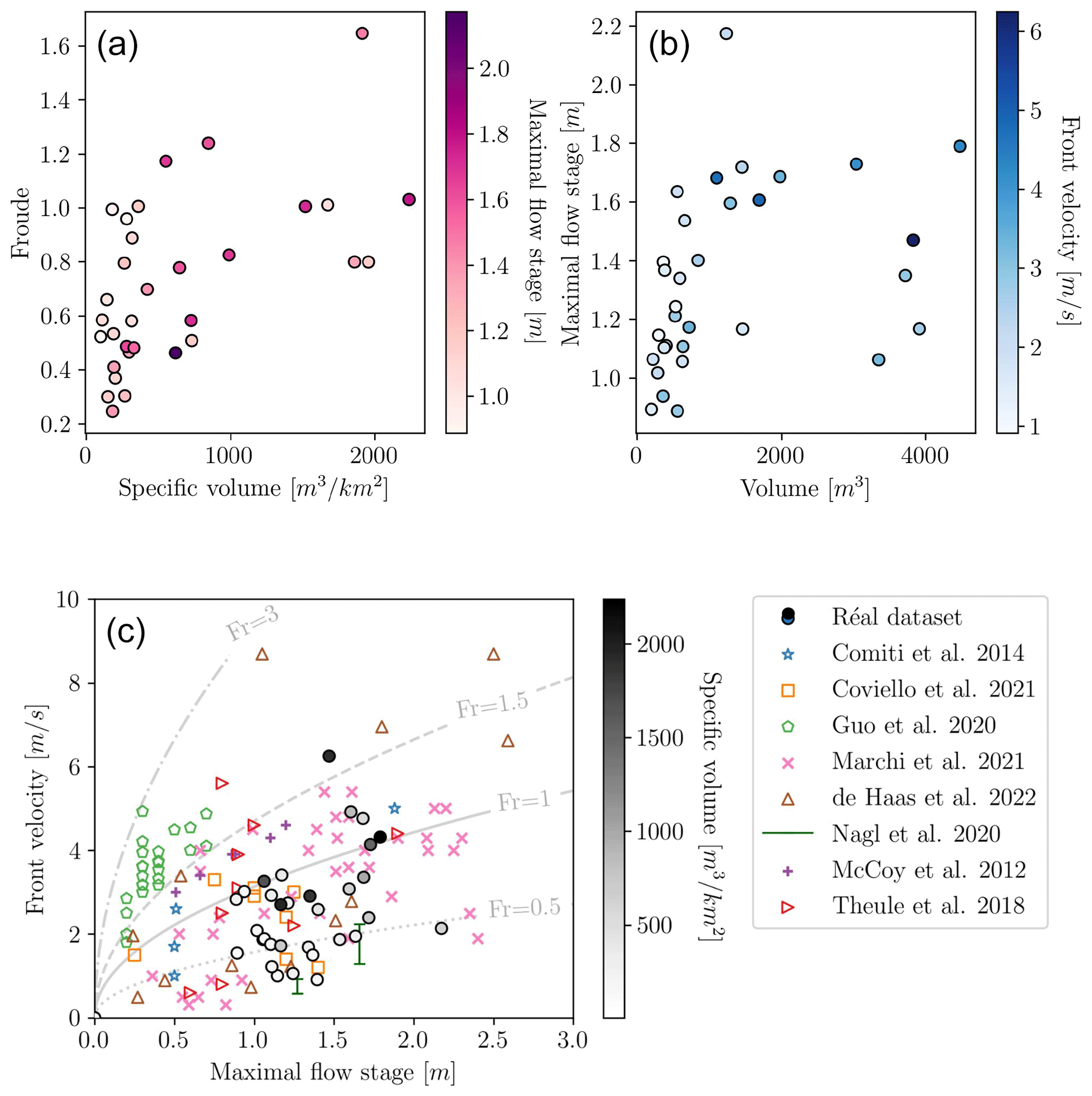
Figure 7 Examples of different relationships that can be explored with this dataset: (a) Froude number vs. specific surge volume, (b) maximum flow height vs. surge volume and (c) front velocity vs. maximum methodology. Data from the literature (Comiti et al., 2014; Coviello et al., 2021; Guo et al., 2020; Marchi et al., 2020; de Haas et al., 2022; Nagl et al., 2020; McCoy et al., 2012; Theule et al., 2018) are displayed in panel (c) to contextualize the values. For Nagl et al. (2020), ranges of maximal and minimal values were taken. For Comiti et al. (2014) and Coviello et al. (2021), values of the flow height were estimated graphically. For Marchi et al. (2020), effective flow height was computed as the difference between flow height at the peak and the start of each surge. Colour mapping is only shown for the Réal dataset. Grey lines display different Froude number relationships.

A slight trend can be seen in Fig. 7a with an increasing Froude number for an increasing specific surge volume. While no clear conclusion can be drawn, there are no surges with large specific volumes (>1000 m³ km⁻²) which have clearly subcritical Froude numbers (all Froude numbers are above 0.8). Most of these surges have near-critical Froude numbers. It seems that debris-flow surges of a large volume require a strong inertial input to flow, as there are no subcritical Froude numbers for volumes of the selected range. Their heavy granular content, increasing their macroscopic viscosity, would cause subcritical, slower flows with high volumes to stop or deconstruct. On the other hand, smaller surges can flow more easily and do not need strong inertial inputs to maintain steady flow. The fact that most of these surges are near critical might in part be due to the sampling at the stations and not the possibility for them to exist: very fast surges with high volume and high inertia are very rare in this catchment. Indeed, the hydrology of the catchment allows for sediment transfers to occur rather often (see Bel, 2017), and the moraine material and steep slopes lead to a low yield criterion of the accumulated sediments. This means that the surges with high volume that are passing at the stations meet the “minimum requirements” for flow. One surge with a supercritical Froude number and high volume is still detected.

If surges would all be of the same hydrograph shape and mixture composition, surge volume would be highly correlated with flow height. However, maximum flow height is quite variable with surge volume (Fig. 7b). This supports the argument that debris-flow hydrographs vary widely.

Similarly, no clear correlation seems to appear between front velocity and flow height (Fig. 7c). Literature data have been displayed, drawing from Comiti et al. (2014), Coviello et al. (2021), Guo et al. (2020), Marchi et al. (2020), de Haas et al. (2022), Nagl et al. (2020), McCoy et al. (2012) and Theule et al. (2018).

Our dataset range has similar Froude numbers as the literature, with most points between Fr=0.5 and Fr=1.5. A point from Simoni et al. (2020) would plot out of the figure (maximal values of velocity: 4 m s⁻¹, flow depth: 4.5 m, rendering a subcritical Froude number of Fr=0.6). Two points from the Marchi et al. (2020) dataset have similar features, notably Froude numbers close to 0.6, and would also plot out of the figure. Most datasets show values similar to the Réal torrent with the notable exception of the dataset provided by Guo et al. (2020) that has generally higher Froude numbers. This is attributed to specificities of this catchment which do not have the slow laminar features that can be found on the reach like the Réal torrent. Overall, all Froude numbers displayed stay under Fr=3.

We interpret this lack of a clear trend or correlation as evidence of varying surge mixture composition between events. The sample size remains however relatively small and site-specific, calling for careful interpretation of these data. We believe it will be of high interest if several other sites could be added to a similar analysis. Fitting a relationship between Froude numbers and surge volume could be a very interesting asset for numerical and experimental modelling.

4 Discussion

4.1 Relationship between surge parameters

Figures 6 and 7 show the ranges of the different features in the database for the Réal torrent. Specific volumes range from 101 to 2237 m³ km⁻². In comparison to specific volumes given by McArdell and Hirschberg (2020), which range from 171 to 7690 m³ km⁻² (catchment size: 11.69 km²), these are much smaller. One of the key reasons why there is such a difference – apart from differences in geological and rheological makeup – is the method employed: classically, available volumes can contain multiple surges and diluted tails, and thus, volumes are not as restrictive as in the method employed in this paper. Specific volumes of the Réal catchment being much smaller is consistent with the difference in the hypothesis of each method. In Coviello et al. (2021), the Gadria catchment monitoring is described and the method employed is much more comparable. In that case, specific volumes of surges range from 35 to 952 m³ km⁻², when taking the catchment size as 6.3 km², which is a range similar to our dataset.

For smaller specific volumes (<1000 m³ km⁻²), Froude numbers range from 0.2 to 1.2 with most surges being clearly subcritical with a value of <0.8. Flow conditions for smaller volumes require less inertial input. For the same specific volume, a wide range of subcritical Froude numbers are found, showing that volume is not the main driver to flowing conditions and that surge mixture composition varies widely in surges of a low volume, i.e. <1000 m³ km⁻². This composition of the mixture changes the mobility of surges.

The initial expectation for Fig. 7b would be that surges of a higher volume render higher maximal flow height. This would be the case if they hydrograph shape was consistent for all events. Debris flows have very variable flow hydrographs (Mitchell et al., 2022, among others) due to a wide range of flow mixture. This leads to similar volumes of debris-flow surges caused by different types of flow hydrographs: a shallow surge which lasts for a long duration or very intense high but short surges.

Figure 7c shows no definitive relationship between proxies for inertial and potential inputs in the flow. This is yet another argument to point out that surge granular content and mixture composition might differ widely from one event to another in the same catchment. The idea that composition of the debris-flow surges changes between events is supported by Hürlimann et al. (2003). A study of the surge content in boulders and coarse grain (Takahashi, 2014) and of their interstitial fluid rheology (Bardou et al., 2003) would be complementary to support this idea but is at the moment not possible with the available data.

4.2 Evidence of the erosion–deposition cycles

In Fig. 5b and d, the valley bottom landforms bear the footprint of high morphological activity due to debris flows, more specifically in the reach between S₁ and S₂ where landforms such as abandoned channels, levees and lobes can be seen (Fig. 5b–c). Figure 8 exemplifies these changes in the channel morphology directly downstream of station S₁ at five different dates. An erosion–deposition cycle of the channel incising and refilling is highlighted over 6 years of field pictures. Such processes explain why many debris flows are measured at station S₁, while many fewer are observed further downstream.

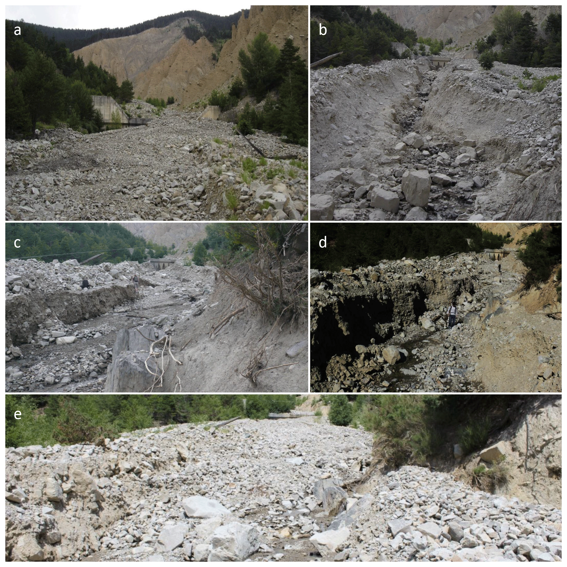
Figure 8 Pictures taken at station S₁ over 6 years: (a) channel filled in June 2009, (b) channel deeply incised in July 2011, (c) channel widened and partially refilled in June 2014 (person for scale), (d) channel further incised in October 2014 (person for scale), and (e) channel refilled in July 2014 (pictures from the authors; Guillaume Piton).

In Fig. 9, volumes of all events are shown along time. If the geomorphic cycle exemplified in Fig. 8 was detectable by this method, pseudo-cycles of cumulated volume surges at station S₁ would be less frequently exported as surges of a higher volume at station S₂ (or as many small-volume surges at S₂ in the following years); i.e. if it were possible to see this geomorphic cycle, the cumulated volumes of the surges passing at S₁ would be found to be equal to the cumulated volume at S₂ over the years. Any amount of the deposits at S₁ or between S₁ and S₂ would then be exported downstream. It can be seen that the two surges reaching station S₃ are indeed of a relatively high volume, but the data lacking between 2015 and 2019 prevent us to draw further observations. With the current data, we can simply conclude that higher volumes of debris-flow pass station S₁ than further downstream. The system is thus storing sediment in the valley through aggradation and/or also exporting sediment volume through a process other than mature debris flows. This is in agreement with the analysis in Theule et al. (2015) which concludes that the sediment activity can be transfer, erosion or deposition in these positions in the reach and in this range of slope (0.11–0.18 m m⁻¹; see Table 1). The applicability of this approach to study the sediment cascade is limited by multiple aspects: the first is that the data of interest are kept at the surge scale and focus on mature debris flows (threshold height of >1 m). Due to the way the data have been processed, studies on global sediment balance are not possible with this analysis, as the events of the bed load and wash load are not taken into account. Indeed, despite its high debris-flow activity, the Réal torrent experiences other processes causing long-term morphological changes such as bed load transport and debris flood that have a meaningful impact on morphological changes and sediment fluxes in various parts of the catchment (Theule et al., 2012).

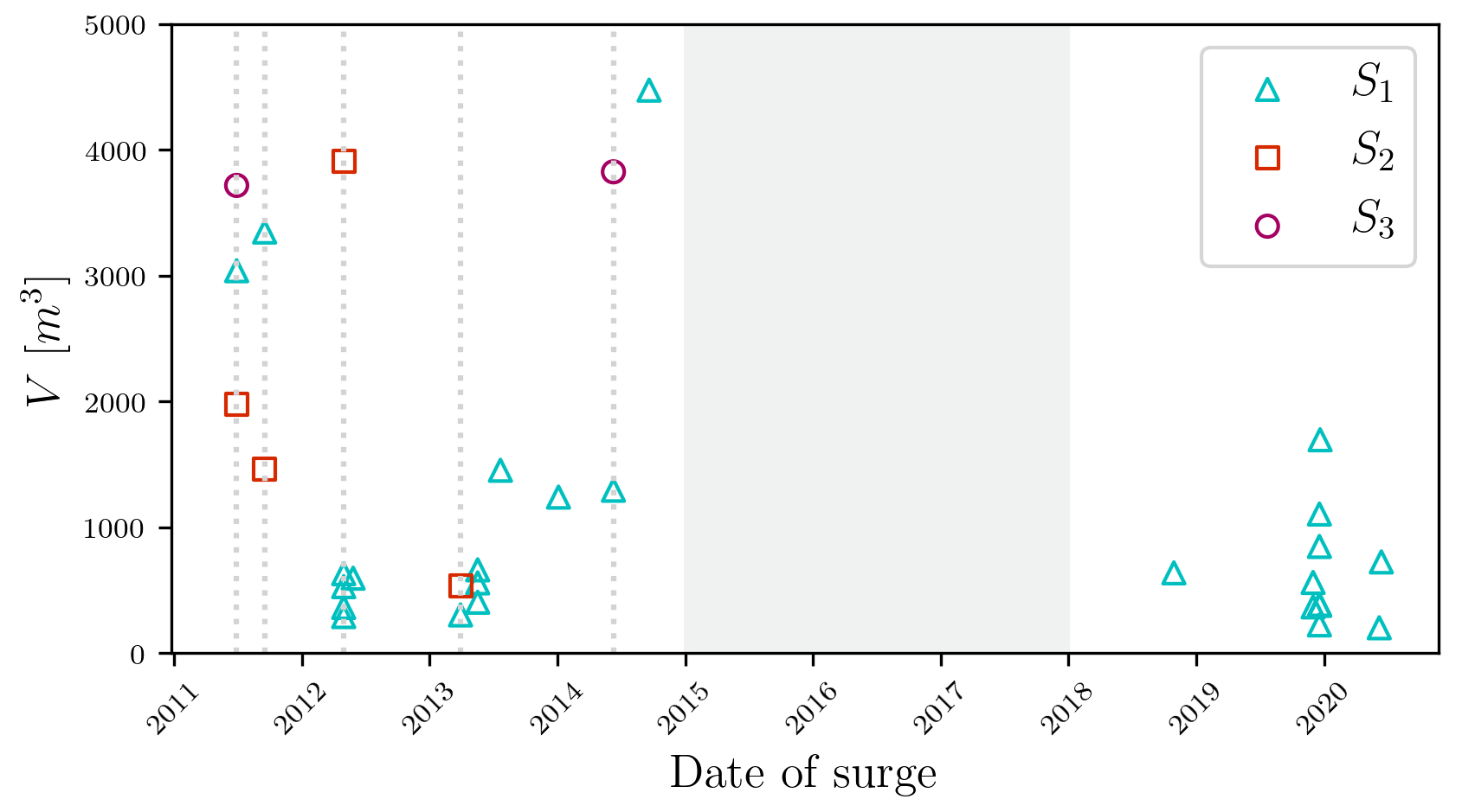
Figure 9 Volume of the surges of mature debris flow passing the stations; the grey area has no data partly due to a faulty sensor invalidating measurements from 2016 until the end of 2017 when the sensor was replaced. No surges were detected in 2015. Dotted grey lines represent dates for which the surge was detected at multiple stations.

4.3 Upstream–downstream transfers of debris-flow surges along the channel

A key interest of having three different monitoring sub-stations in the same torrent is the possibility of studying cascading sediment transfers. Figure 10 shows the analysis of volumes, flow rates, Froude numbers and flow height of each event that could be found at more than one of the stations. One could expect to see consistent relationships between upstream and downstream characteristics, but results are more complicated.

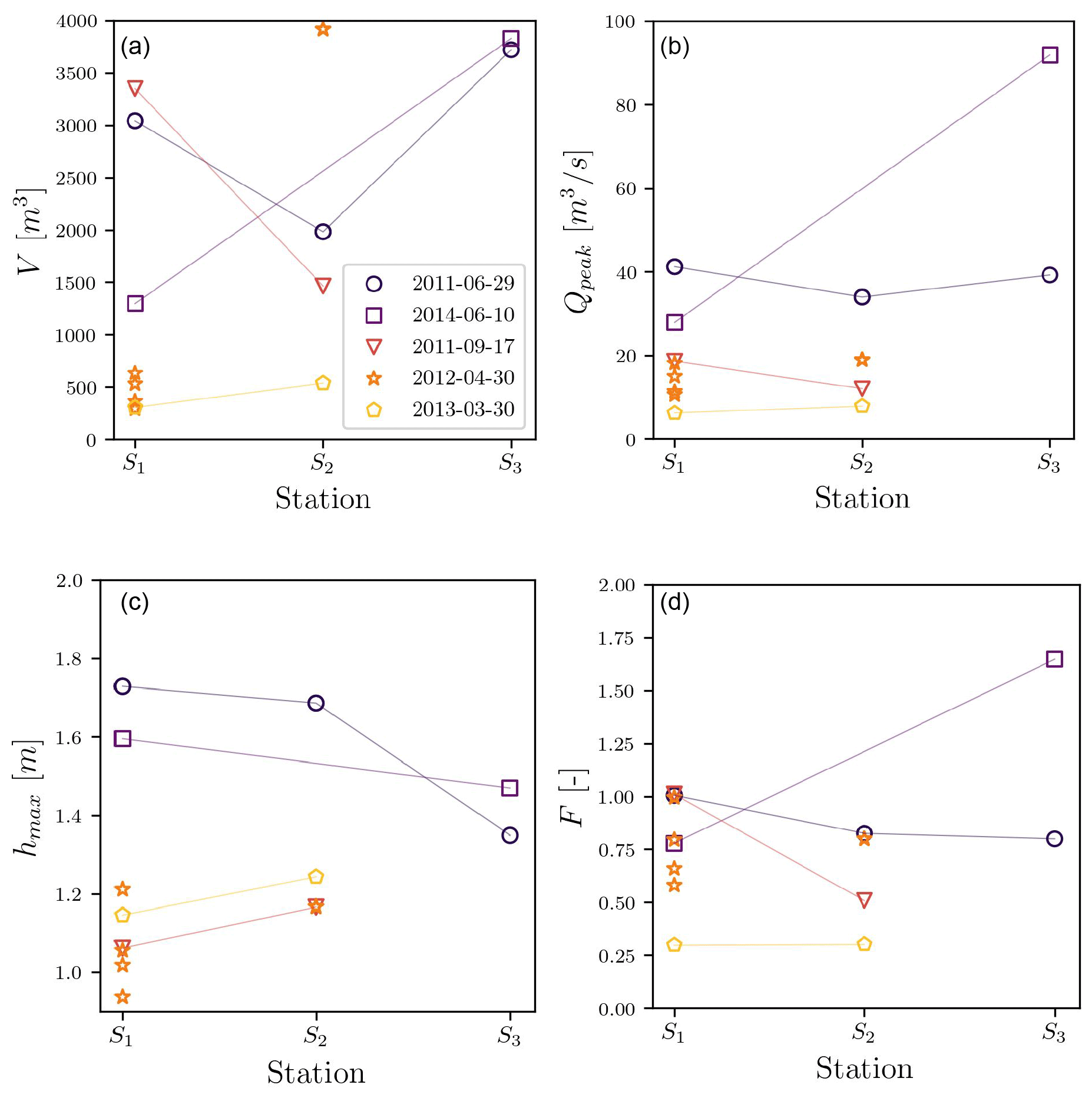
Figure 10 Temporal study for surges detected at two different sub-stations: (a) peak discharge over travelled distance (from the beginning of the channel), (b) volume over travelled distance, (c) maximum flow level and (d) Froude number. Please note that the date format in this figure is year-month-day.

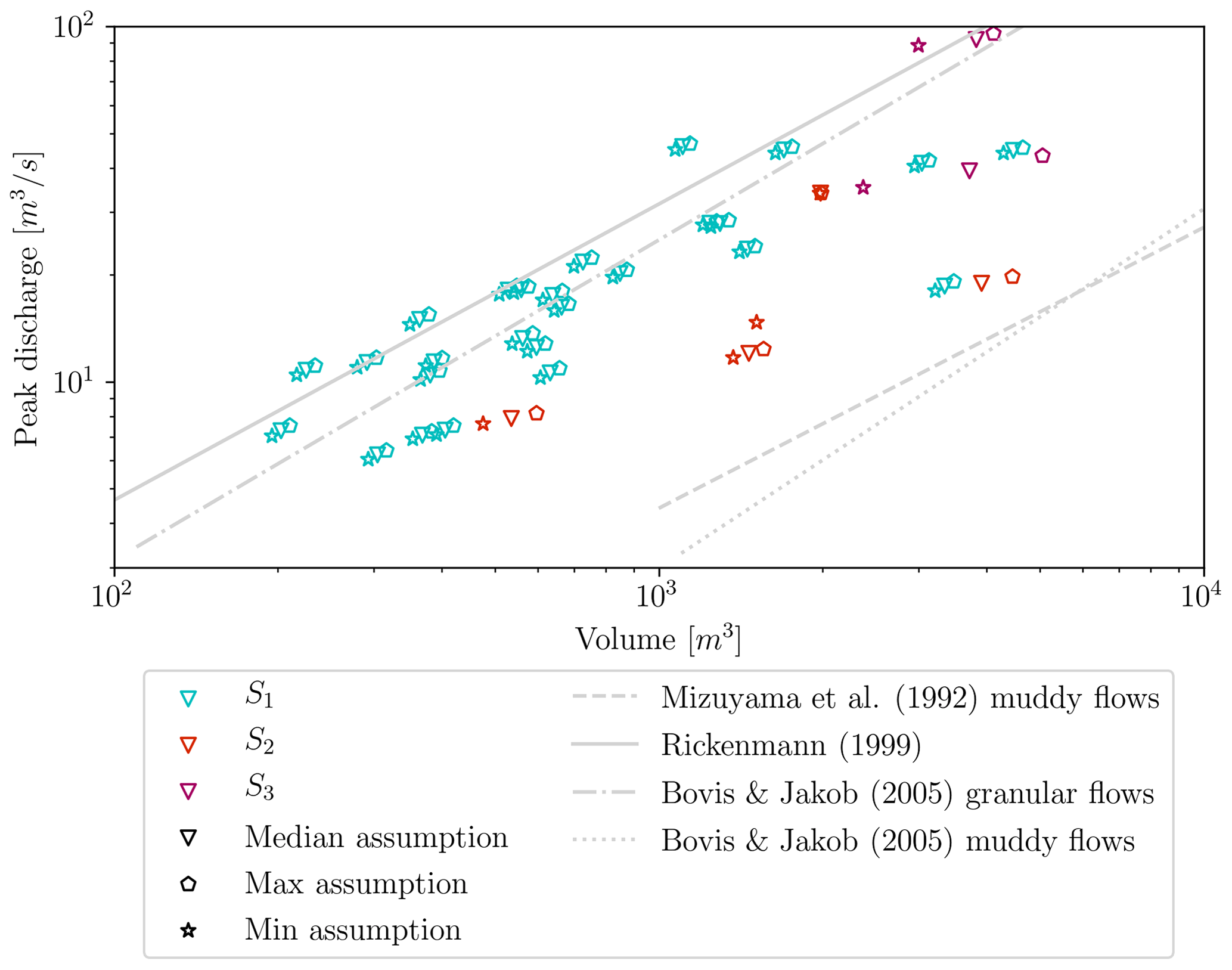
Figure 11 Relationship between debris-flow surge volume and peak discharge for all three stations of the Réal torrent (colour scale for the station and dot shape for the assumptions about the bed level): comparison with empirical fits of datasets from the literature (Bovis and Jakob, 1999; Rickenmann, 1999; Mizuyama et al., 1992).

Volumes passing stations S₁, S₂ and S₃ are generally very different at the same date (Fig. 10). In some cases, the debris-flow surges were growing, recruiting sediment from the bed (V₂>V₁ and/or V₃>V₂), showing the profound morphological changes debris-flow passage can lead to. In other cases, some deposition occurred (V₂<V₁), but erosion might still appear downstream. For the subset of events happening on the same date at the three stations, no particular relationship between the four parameters studied in Fig. 7 was identified.

In Fig. 10a and b, volumes and peak discharge should consistently grow if the surges were consistently eroding from upstream to downstream of the reach. Events like the 30 April 2012 surges show increasing volumes, with a potential agglomeration of the surges between S₁ and S₂ (accumulated volumes at S₁ are smaller than the volume at S₂). This shows deep erosion is possible between the two stations, which is consistent with the morphological changes shown in Fig. 5b. Nonetheless, for this event, peak discharge is not increasing between the two stations. This specificity points out how the pure measurement data and analysis benefit from more specific event data and description.

Similarly, maximum surge depth can also be either lower upstream (30 March 2013, Fig. 10c) or higher at the first station (events of summers 2011 and 2014, Fig. 10c). The Froude number also varies from upstream to downstream with some events having a lower downstream Froude number and others not (Fig. 10d). Froude numbers could be expected to be consistent from upstream to downstream: the ability of the surge to flow would be driven by the interplay between kinetic and potential inputs. Erosion and deposition processes of the surge along the reach will influence the Froude number by changing both the volume and the composition of the surge. This is in agreement with the fact that the slopes in this section are in a sediment transfer regime, as stated by Theule et al. (2015).

The observations of volumes, discharges and surge heights, as well as the much stronger frequency of mature debris flow passing S₁ against those passing S₂ or S₃ (26, 4 and 2, respectively), highlight that strong processes of erosion and deposition occur in the catchment.

While analysing data from three different stations located on such a small and active catchment is interesting, events detected on multiple stations are scarce: most surges detected upstream tend to deposit or to attenuate while travelling such that they are not detected as a mature surge downstream. On the opposite end of this spectrum, a surge that was under the detection threshold on the upstream station might have become fully formed in the downstream stations (see the events of 10 June 2014 and 28 October 2018 that were detected at S₁, not detected at S₂ and again detected at S₃, Table 1).

On the other hand, surges that are detected at multiple stations are also difficult to link to one another, and although volume comparison could be interesting, actual quantitative comparison relies on the hypothesis that the exact same surge between upstream and downstream stations is comparable, i.e. that along the journey, only marginal changes in the process occurred, which is known to be a crude hypothesis of this first work. In essence, the data shown in this paper are interesting because they are actual field observations with quantitative measurements, but the analysis of the catchment sediment transfers is not possible. However, the dataset does demonstrate how strong and intense the processes of erosion and deposition in debris-flow-prone catchments are. An analysis seeking to determine rainfall-triggering conditions of debris flows would for instance draw different conclusions depending on which station is used (but see Bel et al., 2017, partially addressing this issue). We believe that further effort should be put on better understanding not only debris-flow-triggering factors but also propagation through headwaters and intermediate reaches.

Additional multitemporal high-resolution images would help in drawing conclusions on this temporal investigation, and such field campaigns would help answer some of the remaining questions such as the remobilization of the deposited material and evidence of global pseudo-cycles (e.g. Cucchiaro et al., 2018, 2019a, b).

4.4 Analysis of the ranges of the physical characteristics of the events

Comparing the present data to the literature shows the ranges of volumes and flow rates found in the Réal torrent to be consistent with empirical fits proposed in previous works (Bovis and Jakob, 1999; Rickenmann, 1999; Mizuyama et al., 1992), even though the measurements of volumes were done with debris-flow levees in these previous works rather than direct measurements as in our contribution. More precisely, these fits are using the full-scale debris-flow event rather than a single debris-flow surge. In Fig. 11, three values are always plotted for the Réal database: they compare the maximizing, the minimizing and the value of the wetted area chosen to be saved in the database. The effect of the choice of the assumption stays relatively marginal for the upstream station but does have a significant effect on the natural cross-sections, as expected. This highlights the importance of these assumptions in the processing of raw data.

According to Fig. 11, the peak discharge of the Réal catchment for various volumes of debris-flow surges seems closer to the empirical fit related to granular debris flows of Bovis and Jakob (1999) or the fit proposed by Rickenmann (1999). Peak discharges associated with muddy debris flows are lower than those measured at the Réal catchment for equivalent volumes. These results are consistent with the work of Bel (2017), who already showed this concordance using an analysis considering the full debris-flow event with a former version of this methodology.

5 Conclusions

This work is a conceptualization of a widely applicable methodology for debris-flow surge data processing from monitoring stations. A full and simple methodology on debris-flow data processing is presented. The clear goal of this paper is not only to make an initial dataset for the Réal torrent using this methodology available but also to call for collaboration on a common database for debris-flow surge features.

Bulk surge features are investigated including volume, front height, peak discharge and Froude number. This investigation allowed for accessing these hydraulic features of 34 surges gathered from 2011 to 2020 in the Réal torrent catchment (southeastern France, catchment size: 1.3–2 km²). Surge volumes are typically a few thousand cubic metres, peak flow heights range from 1 to 2 m, peak discharge is usually of the order of magnitude of a few dozen of cubic metres per second and their Froude number is near critical.

Access to representative field data will ensure accurate representation of these natural flows. This database is meant to be extended to other monitoring stations to strongly gain in impact in the scientific community. Open access to field data for numerical research can be the bridge needed to close any gaps between the field-driven approaches and the numerical investigations. Research on debris-flow behaviour is growing, and we hope that this initiative will allow for more projects to be born and allow for field observations and numerical computations to evolve conjointly. On top of this, experiences drawn from the post-processing of such data can allow for better, more effective data monitoring in the future (e.g. what type of cross-section to choose, where to install successive stations).