the Creative Commons Attribution 4.0 License.
the Creative Commons Attribution 4.0 License.
 | 22 Mar 2023
Development of a seismic loss prediction model for residential buildings using machine learning – Ōtautahi / Christchurch, New Zealand
Quincy Ma
Pavan Chigullapally
Joerg Wicker
Liam Wotherspoon
This paper presents a new framework for the seismic loss prediction of residential buildings in Ōtautahi / Christchurch, New Zealand. It employs data science techniques, geospatial tools, and machine learning (ML) trained on insurance claims data from the Earthquake Commission (EQC) collected following the 2010–2011 Canterbury earthquake sequence (CES). The seismic loss prediction obtained from the ML model is shown to outperform the output from existing risk analysis tools for New Zealand for each of the main earthquakes of the CES. In addition to the prediction capabilities, the ML model delivered useful insights into the most important features contributing to losses during the CES. ML correctly highlighted that liquefaction significantly influenced building losses for the 22 February 2011 earthquake. The results are consistent with observations, engineering knowledge, and previous studies, confirming the potential of data science and ML in the analysis of insurance claims data and the development of seismic loss prediction models using empirical loss data.
- Article
(7469 KB) - Full-text XML
- BibTeX
- EndNote


In 2010–2011, New Zealand experienced the most damaging earthquakes in its history, known as the Canterbury earthquake sequence (CES). It led to extensive damage to Ōtautahi / Christchurch (hereafter “Christchurch”) buildings, infrastructure, and its surroundings, affecting both commercial and residential buildings. The entire CES led to over NZD 40 billion in total economic losses. Owing to New Zealand's particular insurance structure, the insurance sector contributed to approximately 80 % of the losses for a total of more than NZD 31 billion. NZD 21 billion and NZD 10 billion of the losses as a result of the CES were supported by the private insurers and the Earthquake Commission (EQC) respectively (King et al., 2014; Insurance Council of New Zealand, 2021). Over NZD 11 billion of the losses arose from residential buildings. Approximately 434 000 residential building claims were lodged following the CES and were covered either partially or entirely by the NZ government-backed EQCover insurance scheme (Feltham, 2011; Insurance Council of New Zealand, 2021).
In 2010–2011, EQC provided a maximum cover of NZD 100 000 (+GST) per residential building for any homeowner who previously subscribed to a private home fire insurance (New Zealand Government, 2008). In the process of resolving these claims, EQC collected detailed financial loss data, post-event observations, and building characteristics. The CES was also an opportunity for the NZ earthquake engineering community to collect extensive data on the ground-shaking levels, soil conditions, and liquefaction occurrence throughout wider Christchurch (Cousins and McVerry, 2010; Cubrinovski et al., 2010, 2011; Wood et al., 2011).
This article presents the development of a seismic loss prediction model for residential buildings in Christchurch using data science and machine learning (ML). Firstly, a background on ML and some of its applications in earthquake engineering are provided. Key information regarding ML performance and interpretability is also introduced. Then, details regarding the data that were collected following the CES are given. The challenges posed by the raw data are also highlighted. The following section details the merging process required to enrich the data collected. The data preprocessing steps necessary before the application of ML are then described, and the paper expands on the actual ML model development. It subsequently describes the algorithm selection and model evaluation and presents the insights derived from the previously trained ML model. The next section discusses the current limitations and challenges in the application of ML to real-world loss damage data. Finally, the ML performance is compared to outputs from risk analysis tools available for New Zealand.
2.1 Machine learning applied in earthquake engineering
In recent years, the application of ML to real-world problems increased significantly (Sarker, 2021). Similarly, the use of ML in structural and earthquake engineering gained in popularity. Sun et al. (2020) gave a review of ML applications for building structural design and performance assessment, and Xie et al. (2020) presented an extensive review of the application of ML in earthquake engineering. A few notable relevant ML studies include the quality classification of ground motion records (Bellagamba et al., 2019), the derivation of fragility curves (Kiani et al., 2019), the evaluation of post-earthquake structural safety (Zhang et al., 2018), the classification of earthquake damage to buildings (Mangalathu and Burton, 2019; Mangalathu et al., 2020; Harirchian et al., 2021; Ghimire et al., 2022) and bridges (Mangalathu and Jeon, 2019; Mangalathu et al., 2019), and damage and loss assessment (Kim et al., 2020; Stojadinović et al., 2021; Kalakonas and Silva, 2022a, b).
2.2 Machine learning performance
The performance of an ML model relates to its ability to learn, from a training set, and generalize predictions on unseen data (test data) (Hastie et al., 2009). To achieve this objective, it is important to find a balance between the training error and the prediction error (generalization error). This is known as the bias–variance trade-off (Burkov, 2020; Ng, 2021).
The performance of an ML model might, among other parameters, be improved by using more complex algorithms and feeding more training data to the model. However, despite more training, the accuracy of an ML model will plateau and never surpasses some theoretical limit which is called the Bayes optimal error. It is complex to exactly define where the Bayes optimal error lies for a specific problem. In some cases, the perfect accuracy may not be 100 %. Therefore, it is often simpler to compare the accuracy of an ML model to some baseline performance on a particular task. For some applications ML can be benchmarked against the human-level performance (e.g., image recognition). For others, ML is capable of surpassing human-level performance, as it is able to identify patterns across large data sets. Before evaluating the actual performance of an ML model on a specific task, it is thus important to clarify the context, background, and current baseline performance (Ng, 2021).
2.3 Interpretable machine learning
Depending on the aim and purpose of an ML model, obtaining correct predictions only may be satisfactory. However, recent applications of ML showed that interpretability of the model could help the end user (Honegger, 2018). An ML model can be inspected to identify relationships between input variables, derive insights, and/or find patterns in the data that may be hidden from conventional analysis (Géron, 2022).
Model interpretability is achievable in two main ways. It could come from the possibility for humans to understand the parameters of the algorithm (intrinsic interpretability). This is for example the case for linear regression, which remains interpretable due to its simple structure. For complex models, interpretability could come from methods that analyze the ML model after it has been trained (post hoc methods). One method used to explain predictions from ML models is the SHapley Additive exPlanations (SHAP) tool. SHAP is a methodology originally conceived in game theory for computing the contribution of model features to explain the prediction of a specific instance (Lundberg and Lee, 2017). The SHAP methodology was later extended to the interpretation of tree-based ML algorithms (Lundberg et al., 2019). It can be used to rank the importance of the model features. SHAP relies on the weight of feature attribution rather than on the study of the decrease in model performance. It is thus more robust compared to the permutation of features in tree-based models (Lundberg et al., 2019; Molnar, 2022). Developing post hoc solutions to make complex model decisions understandable to humans remains a topical research endeavor (Du et al., 2020; Molnar, 2022; Ribeiro et al., 2016a, b, 2018).
3.1 Residential building loss data: EQC claims data set
This study uses the March 2019 version of the EQC claims database. Over 95 % of the insurance claims for the CES had been settled by that time. The raw version of the EQC data set contains over 433 500 claims lodged for the CES. Prior to any further data manipulation step, any instances of missing information about the building coordinates and unique property identifier were filtered out as these attributes are essential for mapping and merging. This led to a 5 % loss in the number of claims related to the CES, leaving 412 400 instances in the filtered data set. However, this includes all the claim statuses, among others, claims that were declined and instances settled on associated claims. To maximize the accuracy of the developed loss prediction model, only claims for which the payment was complete were selected. This ensured that the ML model learned from instances for which the claim amount is final. Figure 1 shows the number of instances for different claim statuses. The selection of the complete claims induced a loss of approximately 50 % in the number of instances for the 4 September 2010 and 22 February 2011 events. Figure 2 presents the number of instances for earthquakes in the CES following the selection of settled claims. For a particular earthquake event, it sometimes happened that multiple claims pertaining to the same building were lodged. Figure 2 thus specifically differentiates between the number of claims and the distinct number of buildings affected. Prior to merging and data processing, only four events had more than 10 000 instances (i.e., 4 September 2010, 22 February 2011, 13 June 2011, and 23 December 2011).
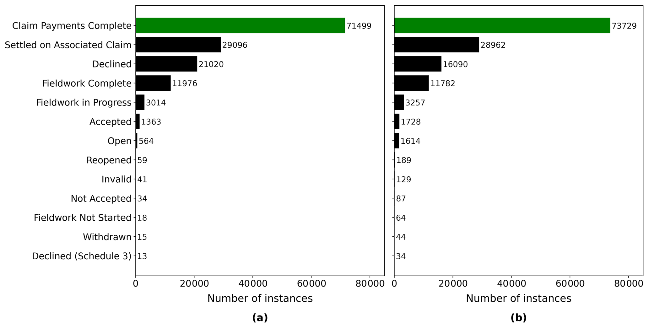
Figure 1Number of instances grouped by the status of the claim: (a) 4 September 2010 and (b) 22 February 2011.
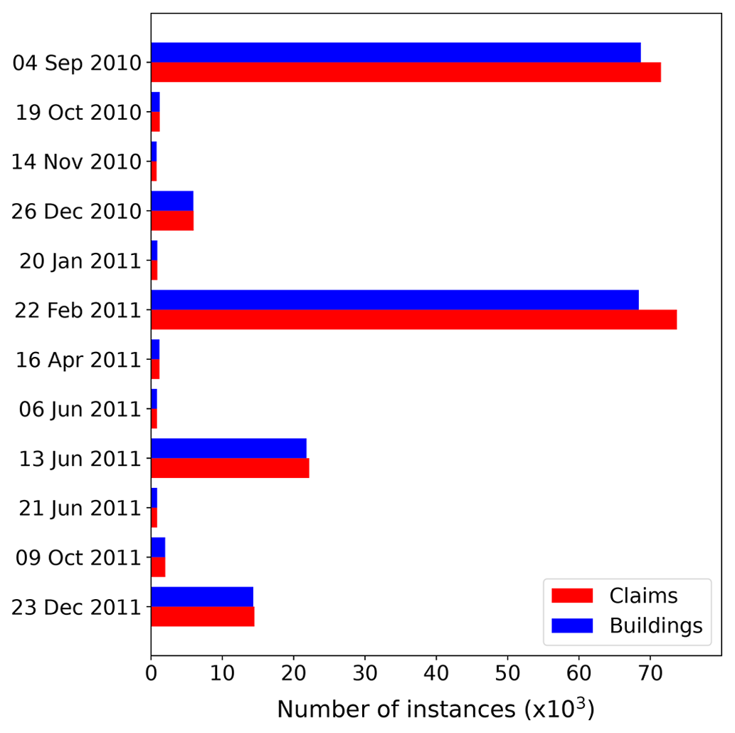
Figure 2Number of claims and property for events in the CES after filtering for ClaimStatus. Only events with more than 1000 instances prior to cleansing are shown.
The EQC claims data set provided included 62 attributes. The data set contained information such as the date of the event; the opening and closing date of a claim; a unique property number; and the claim amount for the building, content, and land. Among the 62 variables, the data set also included information about the building (e.g., construction year, structural system, number of stories). However, for those critical features that identify the building characteristics, more than 80 % of the instances were not collected, as it was not necessary for settlement purposes. Key information such as the building height and primary construction material could not be taken from the EQC data set. The scarce information for building characteristics combined with the necessity to have full data for key variables led to the need to add information from other sources.
3.2 Building characteristics
The RiskScape New Zealand Building inventory data set (NIWA and GNS Science, 2015) had been adopted by this project to deliver critical information on building characteristics. The New Zealand Building inventory collected building asset information for use within the RiskScape software (NIWA and GNS Science, 2017). This data set contained detailed engineering characteristics and other information for every building in New Zealand. Much structural information such as the construction and floor type, the material of the wall cladding, as well as data about the floor area, year of construction of the building, and deprivation index (measure of level of deprivation for an area) could be obtained from the New Zealand Building inventory. However, information about the number of stories was found to be expressed as a float rather than an integer (it seems that the number of stories was calculated from the total floor area of the building divided by the footprint area rather than observed). It was thus decided not to include the number of stories in the model as reliable data, for this attribute was not available.
3.3 Seismic demand
A key input for the damage prediction model is the seismic demand for each individual building. This project utilized recordings from the GeoNet strong motion database for the CES earthquakes at 14 strong motion stations located throughout Christchurch (GeoNet, 2012; Kaiser et al., 2017; Van Houtte et al., 2017). While there are many possible metrics to describe the seismic demand, this study focused on using summary data such as the peak ground acceleration (PGA). For this study, the GeoNet data were interpolated across Christchurch for the four main events using the inverse distance weighted (IDW) interpolation implemented in ArcMap (Esri, 2019).
3.4 Liquefaction occurrence
During the CES, extensive liquefaction occurred during four events: 4 September 2010, 22 February 2011, 13 June 2011, and 23 December 2011. The liquefaction and related land damage were the most significant during the 22 February 2011 event. The location and severity of the liquefaction occurrence were based on interpretation from on-site observations and lidar surveys. Geospatial data summarizing the severity of the observed liquefaction were sourced from the New Zealand Geotechnical Database (NZGD) (Earthquake Commission et al., 2012). The land damage and liquefaction vulnerability due to the CES have been extensively studied. The interested reader is directed to the report from Russell and van Ballegooy (2015).
3.5 Soil conditions
Information on the soil conditions in Christchurch was obtained from the Soil map for the Upper Plains and Downs of Canterbury (Land Resource Information Systems, 2010). The most represented soil types include recent fluvial (RFW, RFT), organic humic (OHM), gley orthic (GOO), brown sandy (BST), pallic perch–gley (PPX), brown orthic (BOA), melanic mafic (EMT), pallic fragic (PXM), and gley recent (GRT).
The final merging approach made use of the Land Information New Zealand (LINZ) NZ Property Titles data set (Land Information New Zealand, 2020a) as an intermediary to constrain the merging process between the EQC and RiskScape data within property boundaries. This was necessary as the coordinates provided by EQC corresponded to the street address (coordinates located close to the street), while RiskScape information was attached to the center of the footprint of a building. Initial merging attempts using built-in spatial join functions and spatial nearest-neighbor joins led to incorrect merging, as in some instances the location of a building from a neighboring property was closer to the EQC coordinates than the actual building (Roeslin et al., 2020).
As the LINZ NZ Property Titles did not directly include information about the street address, it was first necessary to merge the LINZ NZ Addresses data (Land Information New Zealand, 2020b) with the LINZ NZ Property Titles before being able to use the street address information related to a property. Once the LINZ NZ Addresses data (points) and the LINZ NZ Property Titles (polygons) merged, it was found that some properties did not have a matching address point, and some properties had multiple address points within one polygon (see Fig. 3). Polygons with no address point were filtered out. Properties with multiple addresses induced challenges regarding the merging of the EQC claims and RiskScape information. The merging process was thus started with instances of having a unique street address per property.
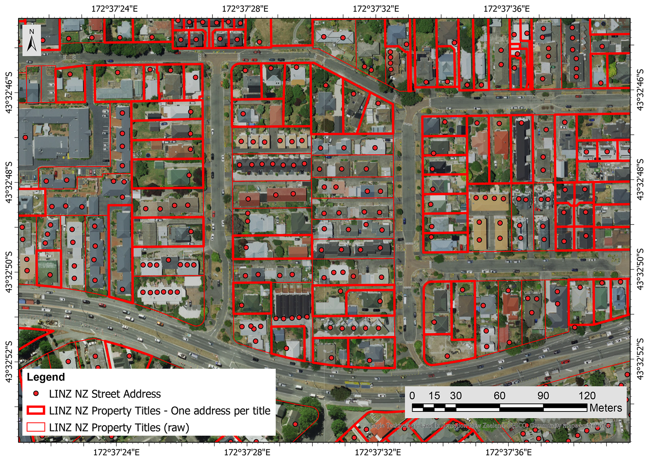
Figure 3Satellite image of urban blocks in Christchurch overlaid with the LINZ NZ Addresses and LINZ NZ Property Titles layers. The polygons with a bold red border represent LINZ NZ property titles having only one street address (background layer from Eagle Technology Group Ltd; NZ Esri Distributor).
The RiskScape database contains information for residential buildings, as well as secondary buildings (e.g., external garages, garden shed). Therefore, some properties contain multiple RiskScape points within a LINZ property title (Fig. 4). All RiskScape points present in a property were merged to LINZ Addresses. The data were then filtered to remove points associated with secondary buildings. The RiskScape database includes two variables related to the building size (i.e., building floor area and building footprint). For properties having only two RiskScape points and under the assumption that the principal dwelling is the building with the largest floor area and footprint on a property, it was possible to filter the data to retain RiskScape information related to the main dwelling only. Some of the properties have three or more RiskScape points. Automatic filtering of the data using the largest building floor area is unreliable for those instances. With the aim of retaining only trusted data, where one street address had more than three RiskScape instances in a property the data were discarded (27.1 % of the selected RiskScape data for Christchurch had three or more points within a LINZ property boundary).
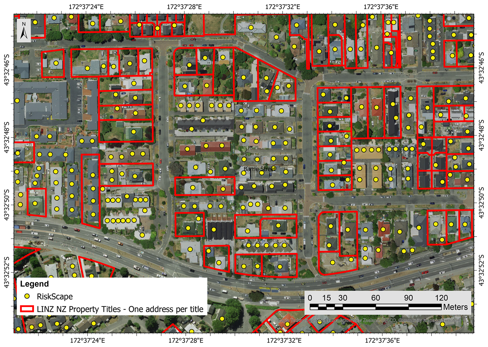
Figure 4Satellite view of an urban block in Christchurch with RiskScape points and selected LINZ NZ Property Titles (background layer from Eagle Technology Group Ltd; NZ Esri Distributor).
In total 7 % of the LINZ property titles have two street address points. As the number of instances used to train a supervised ML model often affects the model accuracy, an attempt was made to retrieve instances that were not collected via the previously mentioned approach. Nevertheless, the philosophy followed here was to put emphasis on the quality of the data rather than the number of points. The effort is focused on retaining the cases when there are two LINZ street addresses and two RiskScape points in the same properties. Following the selection of RiskScape points merged to their unique single LINZ points, the data were appended to the previous RiskScape data set.
Table 1Overview of the action taken depending on the number of LINZ NZ street address and RiskScape points present per LINZ NZ property title.

Table 1 summarizes the merging steps depending on the number of LINZ street address points and RiskScape points per LINZ property title. While the current selection approach is conservative, it ensured each EQC claim can automatically be assigned to the corresponding residential building using the street address. For cases with multiple street addresses or residential buildings within the same property, a manual assignment of RiskScape points to LINZ street address points would enable the inclusion of more instances. However, this was impractical and was applicable to only 4 % of the overall LINZ property titles.
The overall merging process of EQC claims points to LINZ street address points is similar to the process of merging RiskScape to LINZ. The limitations related to the combination of the LINZ NZ street address data with the LINZ NZ property titles apply here as well. Hence, it was only possible to merge EQC claims to street addresses for points contained within LINZ property titles with one street address and to some extent retain claims for properties with two street addresses per title. Once the LINZ NZ street address information was added to RiskScape and EQC, these data sets were merged in Python using the street address as a common field.
The final step of preparing the EQC claims data was to add information related to the seismic demand, the liquefaction occurrence, and the soil conditions. This was achieved within ArcMap (Esri, 2019) by importing each of the data sets as a separate GIS layer. The information contained within each GIS layer was merged with the EQC claims previously combined with RiskScape. Finally, using the street address as a common attribute, the information was combined in one merged data set.
Figure 5 shows the evolution of the number of instances for 4 September 2010 and 22 February 2011 after each step in the merging process. In its original form, the EQC raw data set entails almost 145 000 claims for 4 September 2010 and 144 300 claims for 22 February 2011. Following all the aforementioned merging steps, 38 607 usable instances remain for 4 September 2010 and 42 486 instances for 22 February 2011.
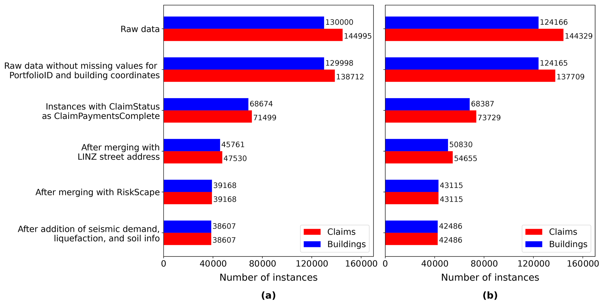
Figure 5The number of data points after each processing step for the event on (a) 4 September 2010 and (b) 22 February 2011.
5.1 Feature filtering
Before fitting an ML model to a data set, it is necessary to remove any instance with missing values, as many of the ML algorithms are unable to make predictions with missing features. Underrepresented categories within attributes are also carefully examined. Categories with few instances introduce challenges for the ML algorithms, as the model will have difficulties “learning” and generalizing for a particular category. In some cases where the meaning is not changed, it is possible to combine instances from different categories. However, whenever a combination of multiple classes is not possible, categories entailing a few instances are removed. This section explains the filtering steps performed on the EQC, RiskScape, and additional attributes.
The EQC claims data set contains an attribute specifying the number of dwellings insured on a claim. To avoid any possible issue with the division of the claim value between the multiple buildings, only claims related to one dwelling were retained. Despite the previous selection of claims with the status Claims Payments Complete (see Sect. 3.1), another attribute capturing the status of the claims indicated that some selected claims were not closed. To avoid any issues that could be caused by non-closed claims, such instances were discarded. Another important attribute from the EQC data set is the building sum insured. At the date of the CES, EQC provided a maximum cover of NZD 100 000 (+GST) or NZD 115 000 (including GST) for a residential dwelling for each natural event (New Zealand Government, 2008). To ensure data integrity for the ML model, only the instances with a maximum cover of exactly NZD 115 000 were selected. Finally, two similar attributes related to the claim amount paid were not exactly matching for some claims. To train the ML model on reliable data, instances where the amount indicated by the building paid attribute did not exactly match with the value of building net incurred were excluded from the data set.
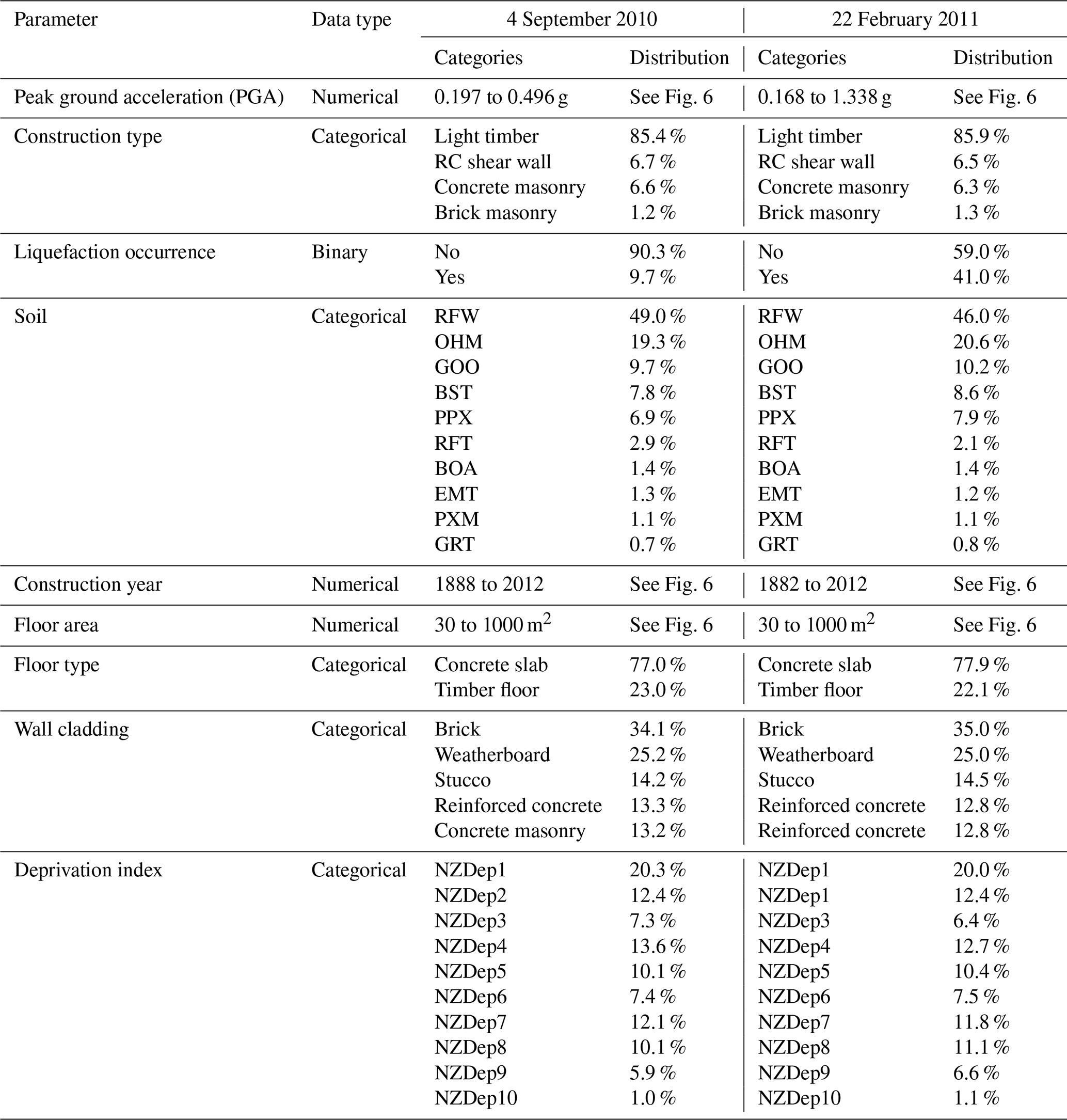
Section 4 presented the merging of the EQC data with additional information related to the building characteristics from RiskScape. Building characteristics encompassed the use category, floor area, construction and floor type, wall and roof cladding, and deprivation index. An exploratory analysis of these attributes revealed that initial filtering was required before further use. The use category was the first RiskScape attribute explored. All instances not having the use category defined as residential dwellings were discarded. Once residential dwellings were selected, the size of the building was examined. The analysis of the floor area revealed the presence of outliers, with values reaching up to 3809 m2 for a single house. To avoid the induction of edge cases in the training set of the ML model, a filtering threshold was set at 1000 m2 (Fig. 6). This led to a minimal loss of instances (0.1 %) but eliminated outliers. The following attribute inspected was related to the material of construction. Table 2 shows the number of instances for each construction type in the merged data set. Light timber was the most prevalent construction type. Conversely, steel braced frame, light industrial, reinforced concrete (RC) moment-resisting frame, and tilt-up panel only appeared in very few instances. Given that these categories have less than 100 instances, it is unlikely ML models can make correct predictions for those construction types. As a result, these underrepresented categories were filtered out of the data set. Selected, along with light timber dwellings, were buildings where the main construction type was classified as RC shear wall, concrete masonry, and brick masonry. While the latter category only entails 347 and 371 instances for 4 September 2010 and 22 February 2011 respectively, it was deemed necessary from an engineering point of view to retain brick masonry as a possible construction type in the model. Along with the building material, RiskScape also entailed information of the floor type. This attribute had two categories: concrete slab and timber floor. Sufficient instances were present in both categories such that no filtering was required. The wall and roof cladding attributes, however, had several underrepresented categories. When possible similar categories were combined, and categories with insufficient entries were discarded. The last attribute sourced from the RiskScape data was the deprivation index. The deprivation index set describes the socioeconomic deprivation of the neighborhood where the building is located. The deprivation index is defined according to 10 categories ranging from 1 (least deprived) to 10 (most deprived) (Atkinson et al., 2020). In total 9 of the 10 categories were well represented. Only the category for the deprivation index 10 (most deprived) had a lower 279 instances for 4 September 2010 and 316 for 22 February 2011. Nevertheless, all data were kept in order to capture the full possible range of values related to the deprivation index attribute.
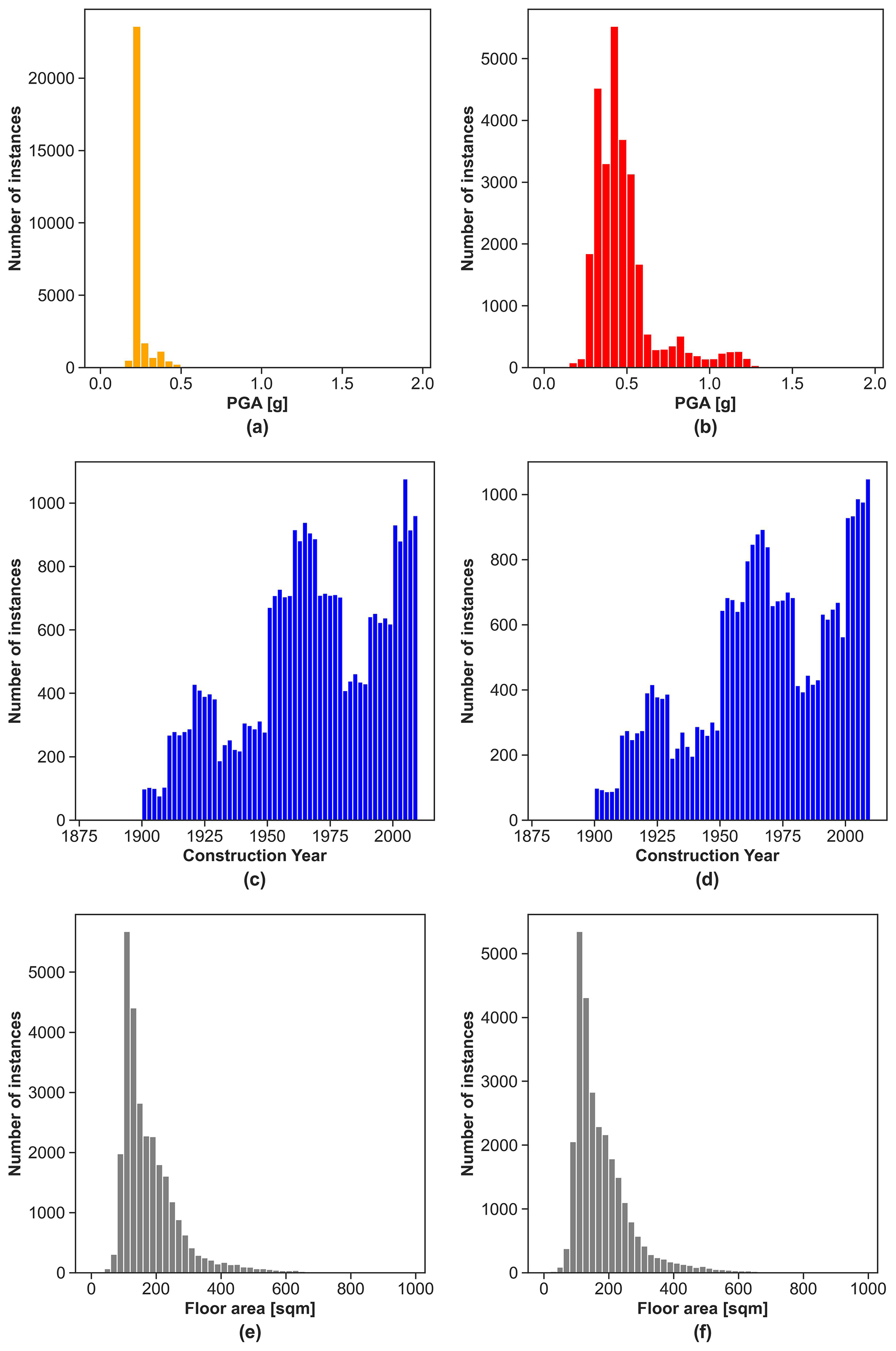
Figure 6Distribution of the numerical attributes: (a) peak ground acceleration (PGA) for 4 September 2010, (b) peak ground acceleration (PGA) for 22 February 2011, (c) construction year for the building claims related to the 4 September 2010 earthquake, (d) construction year for the building claims related to the 22 February 2011 earthquake, (e) floor area for the building claims related to the 4 September 2010 earthquake, and (f) floor area for the building claims related to the 22 February 2011 earthquake.
Table 2Overview of features selected for the model with their distribution.
The final merging included information about the seismic demand, liquefaction occurrence, and soil. To ensure that the ML can generalize, the soil types having less than a hundred instances for 4 September 2010 or 22 February 2011 were removed. Each filtering operation induced a loss in the number of instances. Figure 7 documents the evolution of the number of points through the data preprocessing steps.

Figure 7Evolution of the number of instances after each feature filtering step: (a) 4 September 2010 and (b) 22 February 2011.
5.2 Processing of the target attribute
At the time of the CES in 2010–2011, EQC's liability was capped to the first NZD 100 000 (+GST) (NZD 115 000 including GST) of building damage. Costs above this cap were borne by private insurers if building owners previously subscribed to adequate insurance coverage. Private insurers could not disclose information on private claims settlement, leaving the claims database for this study soft-capped at NZD 115 000 for properties with over NZD 100 000 (+GST) damage. Despite the data set having been previously filtered, an exploratory analysis of the attribute BuildingPaid showed that some instances were above NZD 115 000 and others even negative. To be consistent with the coverage of the EQCover insurance, only instances with BuildingPaid between NZD 0 and NZD 115 000 were selected. Figure 8 shows the distribution of BuildingPaid within the selected range for 4 September 2010 and 22 February 2011. Following the filtering of the BuildingPaid attribute, 28 302 instances remained for 4 September 2010 and 27 537 instances for 22 February 2011.
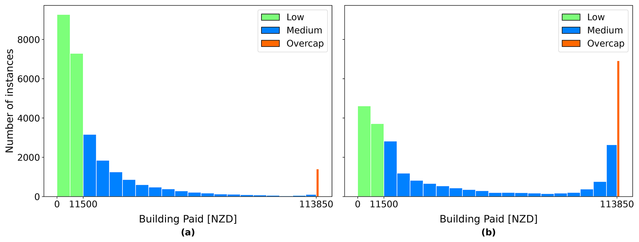
Figure 8Distribution of BuildingPaid after selection of the instances between NZD 0 and NZD 115 000: (a) 4 September 2010 and (b) 22 February 2011.
In the original EQC claims data set, BuildingPaid is a numerical attribute. Initial modeling attempts using BuildingPaid as a numerical target variable produced poor model predictions in terms of both accuracy and ability for generalization. BuildingPaid was thus transformed into a categorical attribute. The thresholds for the cut-offs were chosen according to the EQC definitions related to limits for cash settlement, the Canterbury Home Repair Programme, and the maximum coverage provided (Earthquake Commission, 2019). Any instances with less than and equal to NZD 11 500 were classified as the category “low”, reflecting the limit of initial cash settlement consideration. Next, while the maximum EQC building sum insured was NZD 115 000, it was found that many instances that were overcap showed a BuildingPaid value close to but not exactly at NZD 115 000. In consultation with the risk modeling team at EQC, the threshold for the category “overcap” was set at NZD 113 850, as this represents the actual cap value (nominal cap value minus 1 % excess). Instances with BuildingPaid values between NZD 11 500 and NZD 113 850 were subsequently assigned to the category “medium”. Figure 9 shows the number of instances in each category for 4 September 2010 and 22 February 2011.
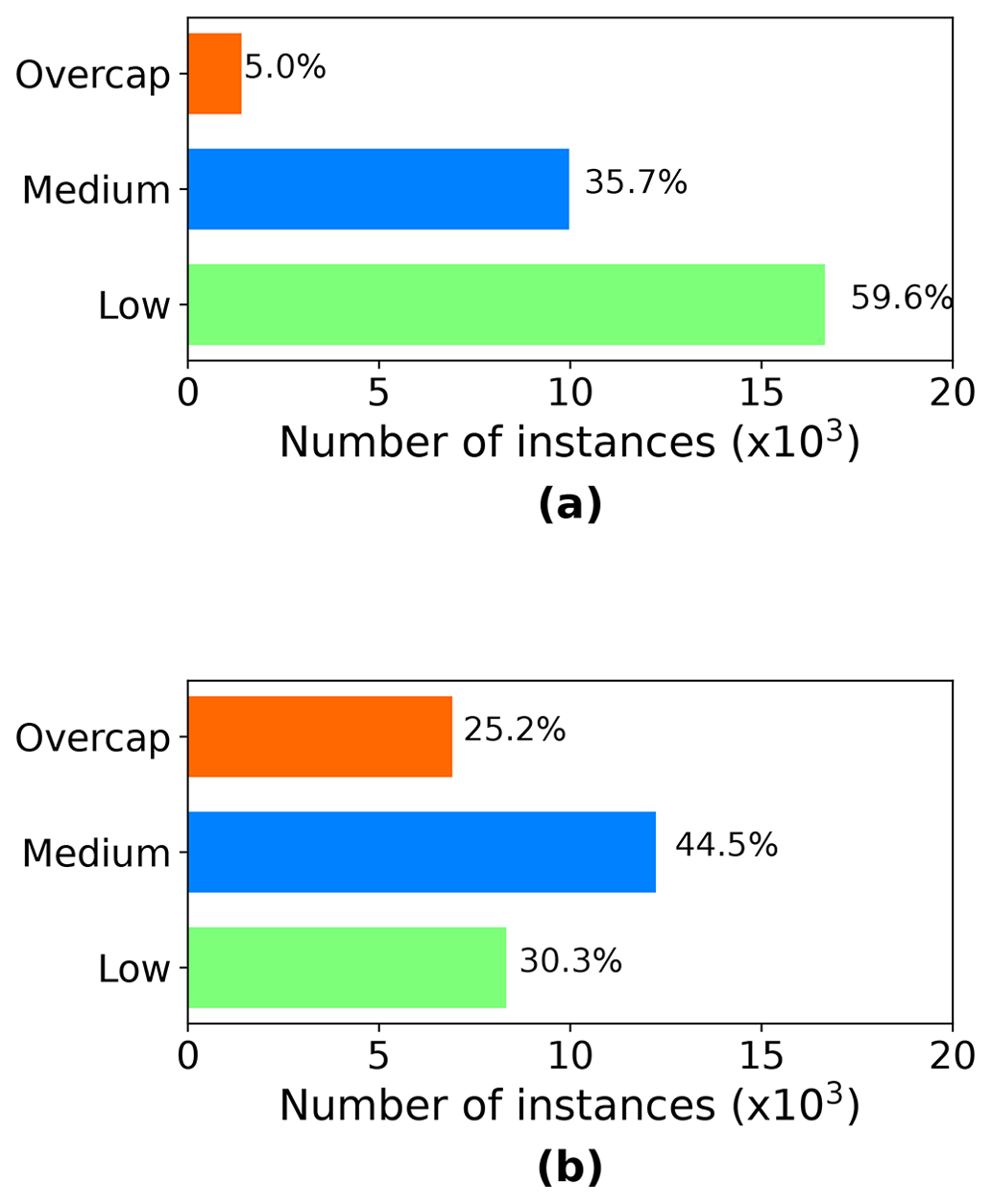
Figure 9Number of instances in BuildingPaid categorical in the filtered data set: (a) 4 September 2010 and (b) 22 February 2011.
The selected data for the model development included nine attributes (PGA, construction type, a flag for liquefaction occurrence, soil type, construction year, floor area, floor type, wall cladding material, deprivation index) plus the target attribute BuildingPaid. The preprocessed data are complete with no missing value for all the instances.
6.1 Training, validation, and test set
For the application of ML, the data were split into three distinct sets, the training, validation (or development), and test set. Figure 10 shows a schematic overview of the splitting and the use of the sets in the development of the ML model. The training, validation, and test sets were coming from the same data set, using 80 % of the data for training, 10 % for validation, and 10 % for testing. The 4 September 2010 preprocessed data had 27 537 instances. Thus, there were 22 030 instances in the training set and 5507 instances in the test set. 22 February 2011 entailed 28 302 instances in total, thus leading to 22 642 examples in the training set and 5660 in the test set. The next most represented events were 13 June and 23 December 2011 (see Fig. 2). Instances from those two events were also merged and preprocessed to enable their use in the training, validation, and testing process.
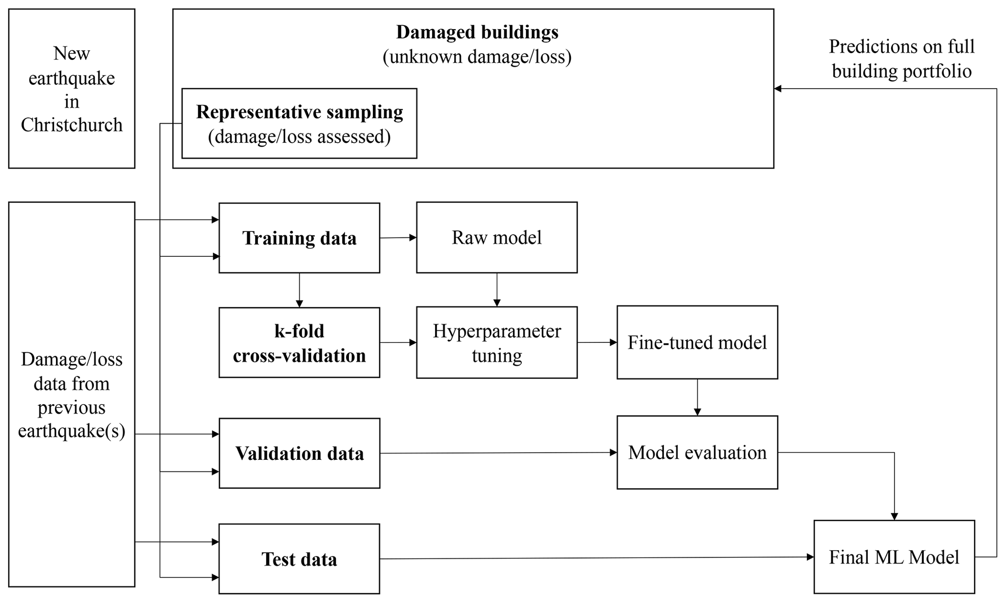
Figure 10Overview of the training, validation, and test data sets and their usage in the development of an ML seismic loss model for Christchurch.
6.2 Handling categorical features
Categorical attributes were transformed into binary arrays for adoption by ML algorithms. For the model in this study, strings in categorical features were first transformed into an ordinal integer using the scikit-learn OrdinalEncoder (Pedregosa et al., 2011). Once converted to integers, the scikit-learn OneHotEncoder (Pedregosa et al., 2011) was used to encode the categorical features as a one-hot numeric array.
6.3 Handling numerical features
Numerical features were checked against each other for correlation prior to the ML training. If two features are correlated, the best practice is to remove one of them. The numerical data were also normalized prior to the training process according to best practice. This step is called feature scaling. The most common feature scaling techniques are min–max scaling (also called normalization) and standardization. Both these techniques can be implemented in scikit-learn (Pedregosa et al., 2011). In this study, a min–max scaling (normalization) approach was used to scale the numerical features.
6.4 Addressing class imbalance
Figure 9a shows the number of instances for each category in the target variable BuildingPaid for the 4 September 2010 data. While the categories low and medium had respectively 16 558 and 9970 instances, the category overcap had only 1404 instances. The overcap category was thus the minority class with a significant difference in the number of instances compared to the two other categories. Training an ML algorithm using the data in this form would lead to poor modeling performance for the overcap category. Thus, before training the model, the imbalanced-learn Python toolbox (Lemaître et al., 2017) was applied to address the class imbalance. The toolbox encompasses several undersampling and oversampling techniques; however not all of them apply to a multiclass problem. The following oversampling and undersampling techniques suitable for multiclass problems were trialed: random oversampling (ROS), cluster centroids (CC), and random undersampling (RUS). For the 4 September 2010 data, ROS delivered the best results regarding the overall model predictions, as well as the prediction for the minority class overcap.
The model was trained using the merged data set, which included information on the model attributes, as well as the target attribute BuildingPaidCat, thus making the training a supervised learning task. Given the nine attributes selected for the model development, the objective of the model was to predict if a building will fall within the category low, medium, or overcap (expressed via the target variable BuildingPaidCat), thus leading to a categorical model for three classes. Several ML algorithms can perform supervised learning tasks for categories (e.g., logistic regression; support vector machine, SVM; random forest, RF; artificial neural networks, ANN). Those algorithms differentiate themselves by their complexity. More complex algorithms can develop more detailed models with a potentially improved prediction performance, but complex algorithms are also more prone to overfitting. For this study, the prediction performance was an essential metric. Nevertheless, the human interpretability of the model was also of significant interest. The goal was to produce a “greybox” model enabling the derivation of insights. In this project, the logistic regression, decision trees, SVM, and random forest were trialed.
Training data were obtained from the four main events in the CES (4 September 2010, 22 February 2011, 13 June 2011, 23 December 2011). Once the model trained, the scikit-learn function RandomizedSearchCV (Pedregosa et al., 2011) was used for the hyperparameter tuning of the model. RandomizedSearchCV was applied in combination with k-fold cross validation. For this exercise of predicting building loss, it was critical to limit the number of false negatives (i.e., actual overcap claims which are not predicted correctly). Using the recall as the scoring for the hyperparameter tuning put the emphasis on the ML model to classify buildings with large losses in the overcap category. Recall was thus chosen as the primary evaluation metric over the accuracy, precision, or F1 score. This paper only presents outputs and findings for 4 September 2010 and 22 February 2011. For findings related to 13 June and 23 December 2011, the reader is directed to Roeslin (2021).
Figure 10 shows the process for the model development. As explained in Sect. 7, multiple ML classification models were trained using data from the four main earthquakes in the CES, and different ML algorithms were trialed. Figure 11 shows confusion matrices for the logistic regression, decision trees, SVM, and random forest trained and validated on data from 22 February 2011. Despite a limited prediction performance, the models trained using the random forest algorithm showed the most promising predictions compared to outputs from the model trained with logistic regression, SVM, and decision tree. The final ML model thus used the random forest algorithm. Following the hyperparameter tuning, the models were evaluated using validation data previously separated from the training set (see Sect. 6.1). Validation sets were also sourced from different events to see how each model would generalize.
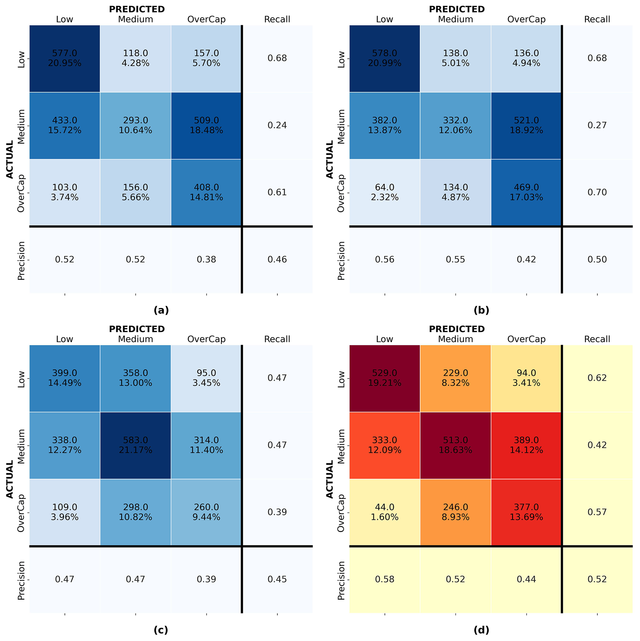
Figure 11Confusion matrices for models trained and validated on data from 22 February 2011: (a) logistic regression, (b) support vector machine (svm), (c) decision tree, and (d) random forest.
Figure 12a and d show the confusion matrix for the random forest model for 4 September 2010 and 22 February 2011 validated on the same event respectively. Figure 12b shows the confusion matrix for the random forest model developed with the 4 September 2010 data and validated on the 22 February 2011 instances. Figure 12c presents the confusion matrix for the random forest model developed with the 22 February 2011 data and applied to the 4 September 2010 instances. For each confusion matrix, the diagonal represents the correct predictions. The top integer numbers in each of the upper-left boxes display the number of instances predicted, and the percentages in the bottom rows represent that instance as a percentage of the entire set. The closest the value on the diagonal sum is to 100 %, the better the prediction. Mistakenly predicted instances are shown off the diagonal. Despite a limited model performance, random forest showed the best overall prediction performance and was deemed the best-performing algorithm in this study.
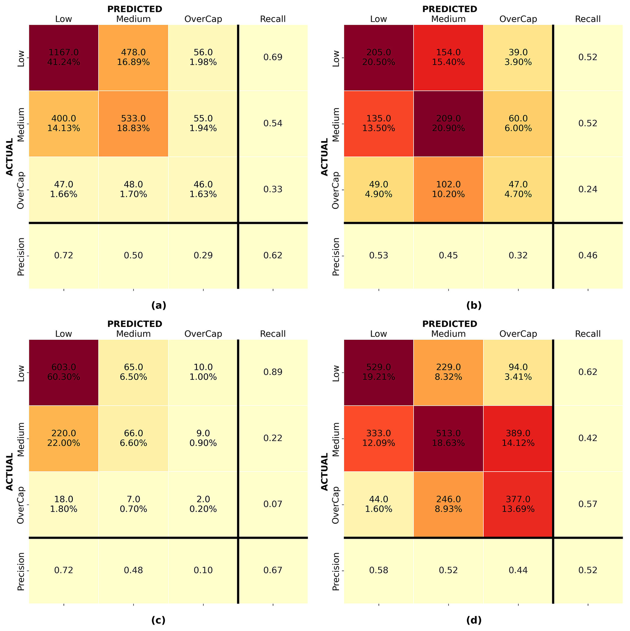
Figure 12Confusion matrices for the random forest algorithm: (a) 4 September 2010 model validated on 4 September 2010, (b) 4 September 2010 model applied to 22 February 2011, (c) 22 February 2011 model applied to 4 September 2010, and (d) 22 February 2011 model validated on 22 February 2011.
Figure 12a shows that model 1, trained and validated on 4 September 2011 data, properly classified over 62 % of the instances. However, it underpredicted 67.4 % of the overcap claims and had difficulties with some of the predictions for the low and medium categories; 40.5 % of the buildings for which a medium claim was lodged were predicted as low, and 28.1 % of the low instances were assigned to the medium category. While the latter might be acceptable for this use case (i.e., leading to larger fund reserves), the former underpredicted the losses. Model 2 (trained and validated on 22 February 2011 data) was only able to classify 52 % of the claims correctly but performed better for overcap cases; 56.5 % of the overcap instances were properly assigned to the overcap category. The better performance of model 2 on overcap instances might be related to the larger number of overcap instances in the training set for the 22 February 2011 event (see Fig. 9). For the medium category the model underpredicted 27.0 % of the medium instances as low. Overall, model 2 underpredicted 22.6 % of the instances in the validation set. Despite the optimization of the model on recall, 36.9 % and 6.6 % of the overcap claims were wrongly assigned to the medium and low categories respectively.
Figure 12b and c help to understand how each model, trained on the 4 September 2010 and 22 February 2011 data respectively, performed when applied to another event. Figure 12b shows that the recall for the overcap category of the model trained on 4 September 2010 applied to 22 February 2011 reached 0.24. For the model trained on the 22 February 2011 data applied to the 4 September 2010 event, the recall was limited to 0.07 for the overcap category with only 7.4 % of the overcap claims being correctly assigned to the overcap category. This shows that besides assessing the performance of a model on a validation set coming from the same earthquake as the training set, it is important to evaluate any ML model on a different earthquake event before making any generalizations.
The SHapley Additive exPlanations (SHAP) post-hoc method was applied to the random forest models for analyzing the relative influence of the different input features. Figure 13 shows the SHAP feature importance for the random forest models for 4 September 2010 and 22 February 2011. The influence of PGA on the residential building losses was highlighted for all the key events of the CES. It was satisfying to observe that ML, which has no physical understanding or prior knowledge related to building damage and loss, was capable of capturing the importance of PGA from empirical data alone.
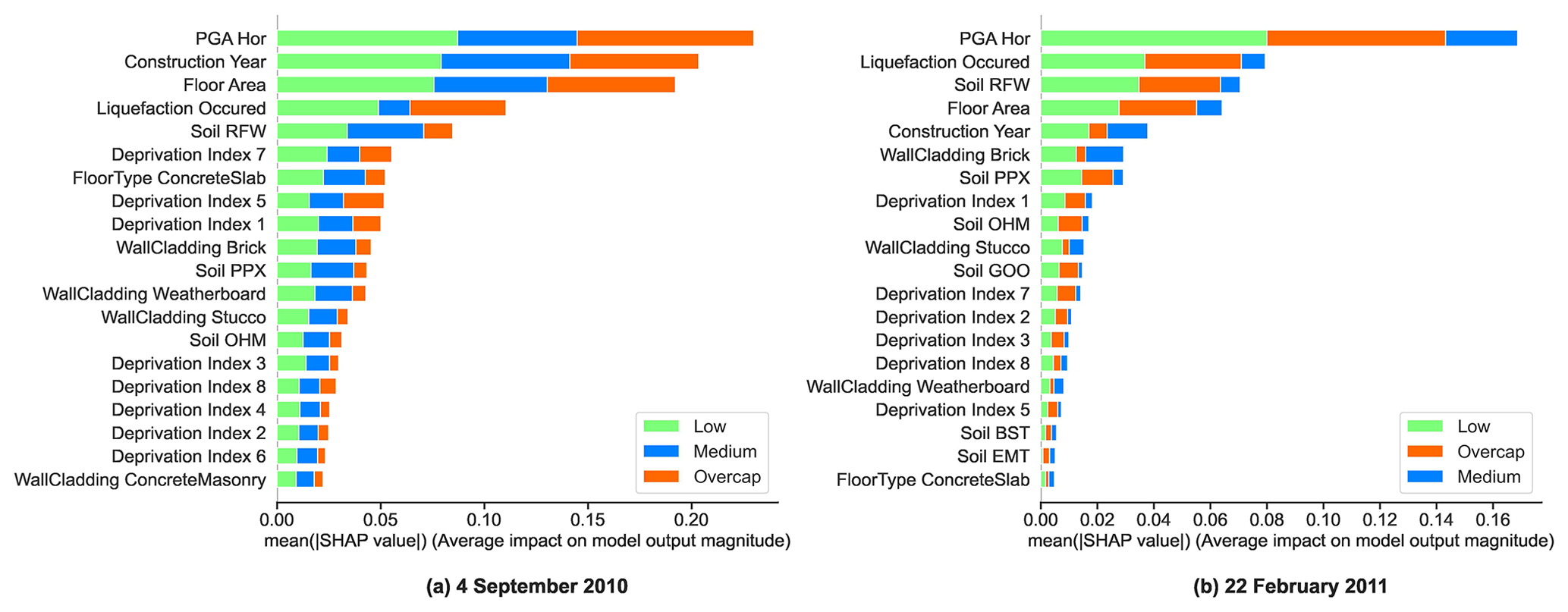
Figure 13SHAP feature importance for the random forest model: (a) 4 September 2010 and (b) 22 February 2011.
For 22 February 2011, PGA significantly stood out and was followed by the liquefaction occurrence and soil type. It thus seemed that the building damage and losses due to the 2011 Christchurch earthquake were driven by liquefaction. This result corroborated the findings from previous studies, which highlighted the influence of liquefaction on building damage for the 22 February 2011 event (Rogers et al., 2015; Russell and van Ballegooy, 2015). The year of construction appeared second for the 4 September 2010 event; however, it was only fifth for the 22 February 2011 event. It is possible that the feature ConstructionYear captured information related to the evolution of the seismic codes which appears more significant for the events less affected by liquefaction.
The study of the feature importance of the ML models seemed to distinguish two types of events: shaking-dominated events such as the 4 September 2010 event and liquefaction-dominated like the 22 February 2011 earthquake.
Once evaluated, a possible scenario was run to test the applicability of the model. As shown in Fig. 10, the proposed framework required the retraining of the ML model, including a sample of buildings from the new earthquake. As claims data were available for the four main earthquakes of the CES, it was possible to demonstrate the applicability of the framework to the Christchurch region using data from previous earthquakes to train an ML model. The date of application chosen for this simulated scenario was in the days following the 13 June 2011 earthquake after the loss assessment on the representative sample was performed. Claims information was thus available for the representative set of buildings (the selection of the best representative set of buildings for the Christchurch portfolio was not part of this case study. It could be done by asking for expert opinions or by using sampling methods as described in Stojadinović et al., 2022). For simplification, it was also assumed that the damage extent and related claims from previous earthquakes were known, thus meaning that the ML model was able to make use of the entire claims data pertaining to the 4 September 2010 and 22 February 2011 events. The ML model was retrained following the steps detailed in Fig. 10.
Figure 14a shows the confusion matrix for model 3, trained and validated on the 4 September 2010 and 22 February 2011 data with the representative sample pertaining to 13 June 2011. The model was trained putting emphasis on recall. On the validation set, the model achieved 0.59 recall on the overcap category with 41.2 % of the overcap instances underpredicted. The model was then applied to the rest of the building portfolio. It predicted 2975 buildings in the low, 3385 in the medium, and 998 buildings in the overcap category. In a real situation, loss assessors could then focus their attention on further assessing subsets of buildings classified in the overcap and medium categories.
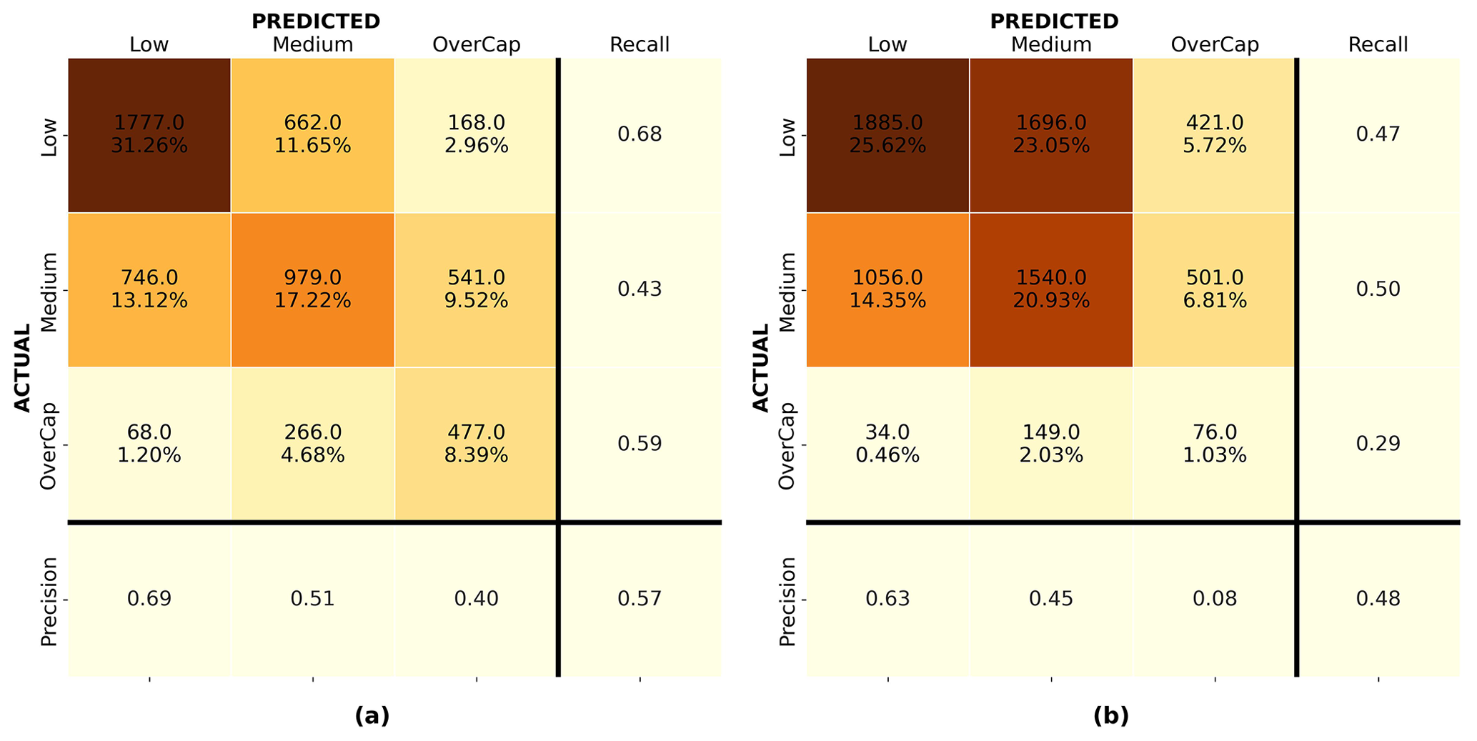
Figure 14(a) Confusion matrix for the random forest algorithm trained and validated on 4 September 2010 and 22 February 2011 data with a representative sample from 13 June 2011 (Model 3) and (b) performance of model 3 on the rest of the building portfolio for the 13 June 2011 earthquake.
As the actual claims are now known, it was possible to assess the model predictions against the ground truth (claims lodged for the 13 June 2011 event). Figure 14b shows the confusion matrix for model 3 applied to the rest of the portfolio of buildings for 13 June 2011. Model 3 underpredicted 70.7 % of the overcap instances with 13.1 % of the overcap claims classified as low. The model had difficulties differentiating between the categories medium and low. A total of 34.1 % of the medium claims were underpredicted as low, meaning that if the loss assessment efforts focused on the medium and overcap categories, 1090 buildings (14.8 % of the portfolio) would not have received appropriate focus in the first instance.
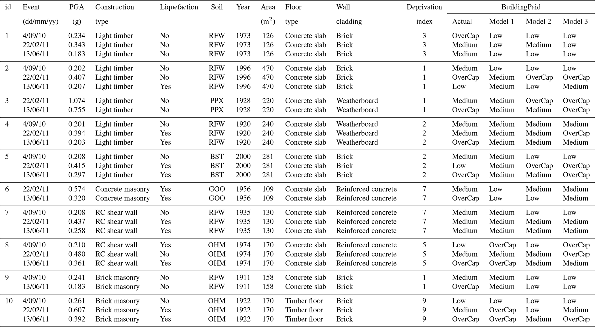
Table 3 presents a sample of 10 buildings for which claims were lodged during the CES. Details about the nine attributes used in the ML model and the actual BuildingPaid are given for each building. The predictions from the random forest model trained on 4 September 2010 (model 1), 22 February 2011 (model 2), and a combination of both events plus a representative sample from 13 June 2011 (model 3) are shown in the last three columns of the table. It is then possible to identify the cases in which the models did not perform well.
Examples 1 to 5 are light timber buildings. Building 1 did not experience any liquefaction occurrence during any of the main events for which a claim was lodged. The only attribute which changed between the events is PGA. Despite a higher level of PGA for the 22 February 2011 event, the reported losses were at the highest for the 4 September 2010 earthquake with the actual value of BuildingPaid being overcap for the 4 September 2010 event and medium for the 22 February and 13 June 2011 events. This example shows that higher PGA levels were not always linked to actual higher claims. Such behavior was difficult to capture in an ML model. Model 3 underpredicted the losses for all the events. The second example presents a light timber building which experienced similar PGA levels during the 4 September 2010 and 13 June 2011 events but higher during the 22 February 2011 earthquake. Liquefaction was only present on 13 June 2011. Model 3 was able to identify the overcap losses of the 22 February 2011 event but overpredicted the losses for the 13 June 2011 earthquake. Building 3 experienced a PGA level above 1 g during the 22 February 2011 earthquake but no liquefaction. Despite the high PGA, the losses were medium'. Model 3 overpredicted the losses for the 22 February 2011 event but correctly predicted the overcap for 13 June 2011. Example 4 has similar PGA levels for 4 September 2010 and 13 June 2011 and higher PGA for 22 February 2011 with liquefaction also present for this event. However, the building losses were different with medium values for 4 September 2010 and 22 February 2011 and overcap for 13 June 2011. None of the models were able to predict the overcap for 13 June 2011. Building 5 experienced liquefaction on both 22 February and 13 June 2011. Despite the higher PGA levels on 22 February 2011, the losses were larger on 13 June 2011. Model 3 accurately predicted the overcap status for 13 June 2011 but overpredicted the losses for 22 February 2011. Cases 6 to 10 show examples having a construction material different from light timber. Despite the higher PGA level during the 22 February 2011 event, building 6 suffered the most losses during the 13 June 2011 earthquake. None of the models were able to assign the 13 June 2011 claim to the overcap category. Nevertheless, with a prediction in medium, model 3 was the closest to reality. Although the PGA levels and liquefaction occurrence were different across the events, the claims related to building 7 were all in the medium category. Besides the prediction for the 4 September 2011 event, model 3 captured the medium level for both the 22 February and 13 June 2011 events. Building 8 suffered major losses during the 13 June 2011 event. Model 3 overpredicted the losses for 4 September 2010 and 22 February 2011 but underpredicted the amount for 13 June 2011. Model 3 also underpredicted building 9. However, for example 9 the claim for 13 June 2011 was overcap despite limited levels of PGA and no presence of liquefaction. Finally, example 10 shows an example where model 3 correctly predicted the losses for each of the events capturing the medium and overcap levels for 22 February and 13 June 2011 respectively.
Despite the thorough attribute filtering, selection, preparation, and model development addressing class imbalance and carefully checking for underfitting and overfitting, the prediction accuracy of the final ML model remained limited. Possible reasons that influence the model performance are discussed in Sect. 12. The error analysis section also highlights the uniqueness of the loss extent related to the CES. Some of the samples presented in Table 3 shows that, for a specific building, higher PGA and the presence of liquefaction did not always lead to the largest claims. This created inherent specificities which were difficult to capture within a global ML model for Christchurch. Nevertheless, the authors are convinced by the potential of applying ML for rapid earthquake loss assessment.
Table 3Sample of 10 buildings for which multiple claims were lodged during the CES. The last three columns show the predictions from the ML models.
There are numerous possible reasons for the limited ML model accuracy. Some are listed here.
Having more direct information collected on site about the building characteristics would improve the completeness of the EQC data set, which could benefit the model performance.
The issues faced during the merging of the EQC data set with RiskScape building characteristics and LINZ information highlighted the need for an improved solution to identify each building in New Zealand. It is believed that the establishment of a unique building identifier common to several databases will introduce consistency, thus opening new opportunities for the application of data science techniques and the derivation of insights.
At the time of the CES, EQC only provided building coverage up to NZD 100 000 (+GST), which led to the EQC data set being capped at NZD 115 000. Losses above the NZD 115 000 threshold were covered by private insurers, given that the building owner subscribed to appropriate private insurance. Any detail for building loss above NZD 115 000 was not available for this study. For 4 September 2010, there was a significant class imbalance between the classes of the target variable with overcap instances being mostly underrepresented. The access to data from private insurances would enlarge the range of the target attribute BuildingPaid, giving more information on the buildings which suffered significant losses.
A more in-depth analysis of the actual value of BuildingPaid might also bring an improved model performance. Taking into account apportionment between the events in the CES would provide a more accurate allocation of loss to each event and enable one to capture more details about overcap instances. To mitigate issues related to sequential damage throughout the CES, the data could be segregated by geographical area where the majority of damage occurred for each event. This might lead to a “cleaner” training set and thus might deliver more accurate predictions.
The prediction accuracy also depends on the attributes present in the model. Section 6 presented the target variable and nine selected model attributes. These attributes were selected based on domain knowledge as possible features that could affect the building losses. There may be other attributes that were not considered in this study that have direct and indirect impacts on the value of a claim. It is thus possible that the inclusion of additional attributes might be beneficial to the overall model accuracy. The introduction of additional parameters related to properties and social factors for example might deliver an improved model accuracy, as well as new insights.
Section 8 and Fig. 12 presented the ML model performance for the random forest model trained on the 4 September 2010 and 22 February 2022 data. Figure 12c showed that the lowest recall score for the overcap category was for the 22 February 2011 model tested on 4 September 2010. Section 2.2 highlighted the importance of providing context and information related to the maximum achievable performance of ML for a specific task. While it was difficult to give an exact value of the Bayes error for this task due to the inherent complexity of loss prediction, it was possible to compare the accuracy of the developed ML model to the performance of current tools employed for the damage and loss prediction.
The outputs of the ML model were compared to predictions obtained from the RiskScape v1.0.3 software (NIWA and GNS Science, 2017). Loss prediction scenarios for the 4 September 2010 and 22 February 2011 events were performed in RiskScape using the hazard information and building data available within the software. RiskScape outputs loss predictions for all the buildings in the Canterbury region. Samples of 25 000 residential buildings located in Christchurch were selected for both the 4 September 2010 and 22 February 2011 events. The buildings in the samples were carefully selected to only encompass buildings for which at least one claim was lodged to EQC during the CES. This later enabled the comparison of the RiskScape software predictions to the actual level of building loss captured by EQC. Figure 15a and b present the confusion matrix of the RiskScape predictions for the 4 September 2010 and 22 February 2011 events respectively. The recall for the overcap category on the 4 September 2010 prediction is 0.08 and 0.11 for the 22 February 2011 earthquake. While the former is slightly better than the worst-performing ML model on 4 September 2010, the latter is significantly lower than any of the recall values achieved for the overcap category using ML for the 22 February 2011 earthquake. Despite limitations in the ML models, ML overall outperformed the RiskScape v1.0.3 software.
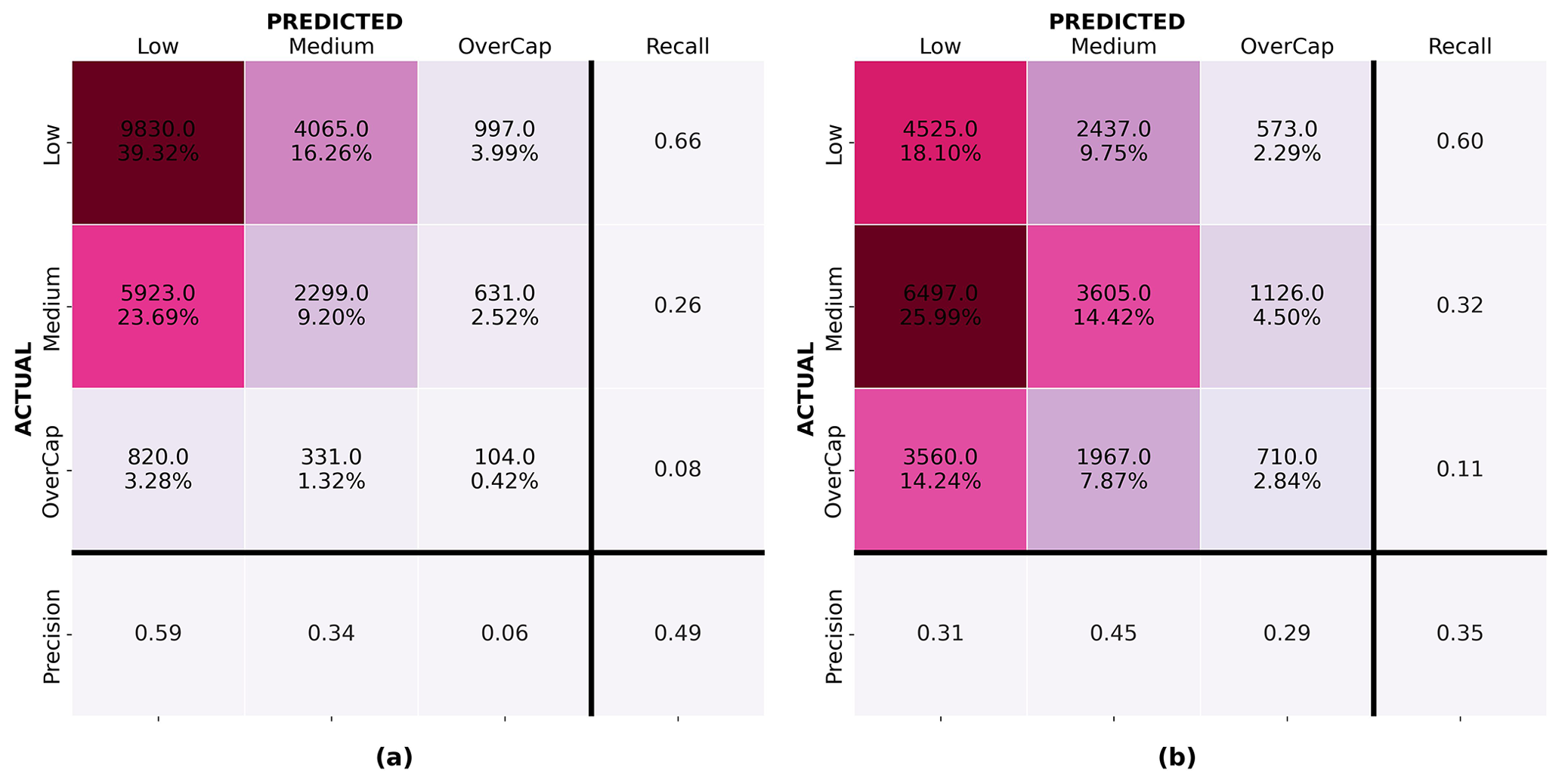
Figure 15Confusion matrices for the predictions from the RiskScape v1.0.3 software on a sample of 25 000 buildings located in Christchurch, New Zealand: (a) predictions for the 4 September 2010 earthquake and (b) predictions for the 22 February 2011 earthquake.
This paper introduced a new framework for the seismic loss prediction of residential buildings. It used residential building insurance claims data collected by the Earthquake Commission following the 2010–2011 Canterbury earthquake sequence to train a machine learning model for loss prediction in residential buildings in Christchurch, New Zealand. The random forest algorithm trained on claims data delivered the most promising outputs. The model application was demonstrated using a scenario whereby an ML model was trained on data from 4 September 2010, 22 February 2011, and a representative sample from 13 June 2011. The ML model was then used to make loss predictions on the rest of the building portfolio. Results from the machine learning model were compared to the performance of current tools for loss modeling. Despite limitations, it was found that the machine learning model outperformed loss predictions obtained using the RiskScape software. It was also shown that machine learning was capable of extracting the most important features that contributed to building loss.
Overall, this research project demonstrated the capabilities and benefits of applying machine learning to empirical data collected following earthquake events. It showed that machine learning was able to extract useful insights from real-world data and outperformed current tools employed for the damage and loss prediction of buildings. It confirmed that data science techniques and machine learning are appropriate tools for the rapid seismic loss assessment.
We signed a confidentiality agreement with EQC, and no information can be shared.
SR: data integration, data preparation, model development, writing; QM: correction and feedback; PC: code review and feedback; JW: feedback on the data science and machine learning part; LW: correction and feedback.
The contact author has declared that none of the authors has any competing interests.
Publisher’s note: Copernicus Publications remains neutral with regard to jurisdictional claims in published maps and institutional affiliations.
This article is part of the special issue “Advances in machine learning for natural hazards risk assessment”. It is not associated with a conference.
We acknowledge the Earthquake Commission, especially the risk modeling team, for the help with data interpretation.
This paper was edited by Vitor Silva and reviewed by Zoran Stojadinovic and one anonymous referee.
Atkinson, J., Salmond, C., and Crampton, P.: NZDep2018 Index of Deprivation, Final Research Report, Final Research Report, University of Otago, Wellington, New Zealand, 1–65, https://www.otago.ac.nz/wellington/otago823833.pdf (last access: 4 March 2023), 2020. a
Bellagamba, X., Lee, R., and Bradley, B. A.: A neural network for automated quality screening of ground motion records from small magnitude earthquakes, Earthq. Spectra, 35, 1637–1661, https://doi.org/10.1193/122118EQS292M, 2019. a
Burkov, A.: Machine Learning Engineering, Vol. 1, True Positive Inc., ISBN 10: 1999579577/ISBN 13: 9781999579579, 2020. a
Cousins, J. and McVerry, G. H.: Overview of strong-motion data from the Darfield earthquake, Bulletin of the New Zealand Society for Earthquake Engineering, 43, 222–227, https://doi.org/10.5459/bnzsee.43.4.222-227, 2010. a
Cubrinovski, M., Green, R. A., Allen, J., Ashford, S., Bowman, E., Bradley, B., Cox, B., Hutchinson, T., Kavazanjian, E., Orense, R., Pender, M., Quigley, M., and Wotherspoon, L.: Geotechnical reconnaissance of the 2010 Darfield (Canterbury) earthquake, Bulletin of the New Zealand Society for Earthquake Engineering, 43, 243–320, https://doi.org/10.5459/bnzsee.43.4.243-320, 2010. a
Cubrinovski, M., Bradley, B., Wotherspoon, L., Green, R., Bray, J., Wood, C., Pender, M., Allen, J., Bradshaw, A., Rix, G., Taylor, M., Robinson, K., Henderson, D., Giorgini, S., Ma, K., Winkley, A., Zupan, J., O'Rourke, T., DePascale, G., and Wells, D.: Geotechnical aspects of the 22 February 2011 Christchurch earthquake, Bulletin of the New Zealand Society for Earthquake Engineering, 44, 205–226, https://doi.org/10.5459/bnzsee.44.4.205-226, 2011. a
Du, M., Liu, N., and Hu, X.: Techniques for interpretable machine learning, Commun. ACM, 63, 68–77, https://doi.org/10.1145/3359786, 2020. a
Earthquake Commission (EQC): Briefing to the Public Inquiry into the Earthquake Commission: Canterbury Home Repair Programme, Tech. Rep., PIES_010.1, 121 pp., EQC, Wellington, New Zealand, https://www.eqc.govt.nz/assets/Publications-Resources/7-v3.-Canterbury-Home-Repair-Programme-Briefing-rs.pdf (last access: 15 November 2022), 2019. a
Earthquake Commission (EQC), Ministry of Business Innovation and Employment (MBIE), and New Zealand Government: New Zealand Geotechnical Database (NZGD), https://www.nzgd.org.nz/Default.aspx (last access: 8 November 2022), 2012. a
Esri: ArcGIS Desktop 10.7.1, Environmental Systems Research Institute, Redlands, CA, 2019. a, b
Feltham, C.: Insurance and reinsurance issues after the Canterbury earthquakes, Parliamentary Library Reasearch Paper, 1–2, https://www.parliament.nz/resource/en-NZ/00PlibCIP161/e9e4aba0e5a8b0eccf517d16183735b2f3c871a5 (last access: 4 March 2023), 2011. a
GeoNet: GeoNet Strong Motion Data Tool, https://strongmotion.geonet.org.nz/ (last access: 20 June 2021), 2012. a
Géron, A.: Hands-On Machine Learning with Scikit-Learn, Keras, and TensorFlow, O'Reilly Media, 3rd edn., ISBN: 9781098122461, 1098122461, 2022. a
Ghimire, S., Guéguen, P., Giffard-Roisin, S., and Schorlemmer, D.: Testing machine learning models for seismic damage prediction at a regional scale using building-damage dataset compiled after the 2015 Gorkha Nepal earthquake, Earthq. Spectra, 38, 2970–2993, https://doi.org/10.1177/87552930221106495, 2022. a
Harirchian, E., Kumari, V., Jadhav, K., Rasulzade, S., Lahmer, T., and Das, R. R.: A synthesized study based on machine learning approaches for rapid classifying earthquake damage grades to rc buildings, Appl. Sci.-Basel, 11, 7540, https://doi.org/10.3390/app11167540, 2021. a
Hastie, T., Tibshirani, R., and Friedman, J.: The Elements of Statistical Learning, Springer Series in Statistics, Springer, New York, https://doi.org/10.1007/978-0-387-84858-7, 2009. a
Honegger, M.: Shedding Light on Black Box Machine Learning Algorithms, PhD thesis, Karlsruhe Institue of Technology, Germany, arXiv [preprint], https://doi.org/10.48550/arXiv.1808.05054, 15 August 2018. a
Insurance Council of New Zealand (ICNZ): Canterbury Earthquakes, https://www.icnz.org.nz/natural-disasters/canterbury-earthquakes/, last access: 3 October 2021. a, b
Kaiser, A., Van Houtte, C., Perrin, N., Wotherspoon, L., and Mcverry, G.: Site Characterisation of GeoNet Stations for the New Zealand Strong Motion Database, Bulletin of the New Zealand Society for Earthquake Engineering, 50, 39–49, https://doi.org/10.5459/bnzsee.50.1.39-49, 2017. a
Kalakonas, P. and Silva, V.: Earthquake scenarios for building portfolios using artificial neural networks: part II—damage and loss assessment, B. Earthq. Eng., https://doi.org/10.1007/s10518-022-01599-2, 2022a a
Kalakonas, P. and Silva, V.: Seismic vulnerability modelling of building portfolios using artificial neural networks, Earthq. Eng. Struct. D., 51, 310–327, https://doi.org/10.1002/eqe.3567, 2022b. a
Kiani, J., Camp, C., and Pezeshk, S.: On the application of machine learning techniques to derive seismic fragility curves, Comput. Struct., 218, 108–122, https://doi.org/10.1016/j.compstruc.2019.03.004, 2019. a
Kim, T., Song, J., and Kwon, O. S.: Pre- and post-earthquake regional loss assessment using deep learning, Earthq. Eng. Struct. D., 49, 657–678, https://doi.org/10.1002/eqe.3258, 2020. a
King, A., Middleton, D., Brown, C., Johnston, D., and Johal, S.: Insurance: Its Role in Recovery from the 2010–2011 Canterbury Earthquake Sequence, Earthq. Spectra, 30, 475–491, https://doi.org/10.1193/022813EQS058M, 2014. a
Land Information New Zealand (LINZ): NZ Property Titles, LINZ Data Service [data set], https://data.linz.govt.nz/layer/50804-nz-property-titles/ (last access: 5 June 2022), 2020a. a
Land Information New Zealand (LINZ): NZ Street Address, LINZ Data Service [data set], https://data.linz.govt.nz/layer/53353-nz-street-address/ (last access: 5 June 2022), 2020b. a
Land Resource Information Systems (LRIS): Soil map for the Upper Plains and Downs of Canterbury, LRIS [data set], https://doi.org/10.26060/1PGJ-JE57, 2010. a
Lemaître, G., Nogueira, F., and Aridas, C. K.: Imbalanced-learn: A Python Toolbox to Tackle the Curse of Imbalanced Datasets in Machine Learning, J. Mach. Learn. Res., 18, 1–5, http://jmlr.org/papers/v18/16-365.html (last access: 16 October 2021), 2017. a
Lundberg, S. M. and Lee, S.-I.: A Unified Approach to Interpreting Model Predictions, in: Advances in Neural Information Processing Systems 30 (NIPS 2017), edited by: Guyon, I., Von Luxburg, U., Bengio, S., Wallach, H., Fergus, R., Vishwanathan, S., and Garnett, R., Curran Associates, Inc., https://proceedings.neurips.cc/paper/2017/file/8a20a8621978632d76c43dfd28b67767-Paper.pdf (last access: 20 October 2020), 2017. a
Lundberg, S. M., Erion, G. G., and Lee, S.-I.: Consistent Individualized Feature Attribution for Tree Ensembles, 2017 ICML Workshop, arXiv [preprint], https://doi.org/10.48550/arXiv.1802.03888, 7 March 2019. a, b
Mangalathu, S. and Burton, H. V.: Deep learning-based classification of earthquake-impacted buildings using textual damage descriptions, Int. J. Disast. Risk Re., 36, 101111, https://doi.org/10.1016/j.ijdrr.2019.101111, 2019. a
Mangalathu, S. and Jeon, J.-S.: Machine Learning–Based Failure Mode Recognition of Circular Reinforced Concrete Bridge Columns: Comparative Study, J. Struct. Eng., 145, 04019104, https://doi.org/10.1061/(ASCE)ST.1943-541X.0002402, 2019. a
Mangalathu, S., Hwang, S. H., Choi, E., and Jeon, J. S.: Rapid seismic damage evaluation of bridge portfolios using machine learning techniques, Eng. Struct., 201, 109785, https://doi.org/10.1016/j.engstruct.2019.109785, 2019. a
Mangalathu, S., Sun, H., Nweke, C. C., Yi, Z., and Burton, H. V.: Classifying earthquake damage to buildings using machine learning, Earthq. Spectra, 36, 183–208, https://doi.org/10.1177/8755293019878137, 2020. a
Molnar, C.: Interpretable Machine Learning. A Guide for Making Black Box Models Explainable, ISBN-13: 979-8411463330 https://christophm.github.io/interpretable-ml-book/, last access: 13 June 2022. a, b
New Zealand Government: Earthquake Commission Act 1993 – 1 April 2008, https://www.legislation.govt.nz/act/public/1993/0084/7.0/DLM305968.html (last access: 14 July 2022), 2008. a, b
Ng, A.: CS230 Deep Learning - C3M1: ML Strategy (1), CS230 Deep Learning class, Stanford University, https://cs230.stanford.edu/files/C3M1.pdf (last access: 3 July 2022), 2021. a, b
NIWA and GNS Science: RiskScape - Asset Module Metadata, GitHub [data set], https://bit.ly/RiskScapeAssetModuleMetadata20151204 (last access: 25 November 2022), 2015. a
NIWA and GNS Science: RiskScape, https://www.riskscape.org.nz/ (last access: 6 December 2022), 2017. a, b
Pedregosa, F., Varoquaux, G., Gramfort, A., Michel, V., Thirion, B., Grisel, O., Blondel, M., Prettenhofer, P., Weiss, R., Dubourg, V., Vanderplas, J., Passos, A., Cournapeau, D., Brucher, M., Perrot, M., and Duchesnay, E.: Scikit-learn: Machine Learning in Python, J. Mach. Learn. Res., 12, 2825–2830, https://www.jmlr.org/papers/volume12/pedregosa11a/pedregosa11a.pdf (last access: 15 March 2022), 2011. a, b, c, d
Ribeiro, M. T., Singh, S., and Guestrin, C.: “Why Should I Trust You?”: Explaining the Predictions of Any Classifier, in: Proceedings of the 2016 Conference of the North American Chapter of the Association for Computational Linguistics: Demonstrations, San Diego, California, 1135–1144, https://doi.org/10.18653/v1/N16-3020, 2016a. a
Ribeiro, M. T., Singh, S., and Guestrin, C.: Model-Agnostic Interpretability of Machine Learning, in: 2016 ICML Workshop on Human Interpretability in Machine Learning (WHI 2016), New York, NY, arXiv [preprint], https://doi.org/10.48550/arXiv.1606.05386, 16 June 2016b. a
Ribeiro, M. T., Singh, S., and Guestrin, C.: Anchors: High-Precision Model-Agnostic Explanations, in: Proceedings of the AAAI Conference on Artificial Intelligence (AAAI'18), 32, 1527–1535, https://doi.org/10.1609/aaai.v32i1.11491, 2018. a
Roeslin, S.: Predicting Seismic Damage and Loss for Residential Buildings using Data Science, PhD thesis, University of Auckland, Auckland, New Zealand, https://hdl.handle.net/2292/57074 (last access: 18 December 2022), 2021. a
Roeslin, S., Ma, Q., Wicker, J., and Wotherspoon, L.: Data Integration for the Development of a Seismic Loss Prediction Model for Residential Buildings in New Zealand, in: Machine Learning and Knowledge Discovery in Databases, edited by: Cellier, P. and Driessens, K., Springer, Cham, Switzerland, Comm. Com. Inf. Sc., 1168, 88–100, https://doi.org/10.1007/978-3-030-43887-6_8, 2020. a
Rogers, N., van Ballegooy, S., Williams, K., and Johnson, L.: Considering Post-Disaster Damage to Residential Building Construction - Is Our Modern Building Construction Resilient?, in: 6th International Conference on Earthquake Geotechnical Engineering (6ICEGE), Christchurch, New Zealand, 1–4 November 2015, https://www.issmge.org/publications/publication/considering-postdisaster-damage-to-residential-building-construction-is- our-modern-building-construction-resilient (last access: 4 March 2023), 2015. a
Russell, J. and van Ballegooy, S.: Canterbury Earthquake Sequence: Increased Liquefaction Vulnerability assessment methodology, Tonkin & Taylor Ltd, Auckland, New Zealand, Tech. rep., 0028-1-R-JICR-2015, 204 pp., https://www.eqc.govt.nz/assets/Publications-Resources/CES- Increased-Liquefaction-Vulnerability-Assessment-Methodology -T+T-Report.pdf (last access: 23 April 2022), 2015. a, b
Sarker, I. H.: Machine Learning: Algorithms, Real-World Applications and Research Directions, SN Computer Science, 2, 160, https://doi.org/10.1007/s42979-021-00592-x, 2021. a
Stojadinović, Z., Kovačević, M., Marinković, D., and Stojadinović, B.: Rapid earthquake loss assessment based on machine learning and representative sampling, Earthq. Spectra, 38, 152–177, https://doi.org/10.1177/87552930211042393, 2022. a
Sun, H., Burton, H. V., and Huang, H.: Machine Learning Applications for Building Structural Design and Performance Assessment: State-of-the-Art Review, Journal of Building Engineering, 33, 101816, https://doi.org/10.1016/j.jobe.2020.101816, 2020. a
Van Houtte, C., Bannister, S., Holden, C., Bourguignon, S., and Mcverry, G.: The New Zealand strong motion database, Bulletin of the New Zealand Society for Earthquake Engineering, 50, 1–20, https://doi.org/10.5459/bnzsee.50.1.1-20, 2017. a
Wood, C. M., Cox, B. R., Wotherspoon, L. M., and Green, R. A.: Dynamic site characterization of Christchurch strong motion stations, Bulletin of the New Zealand Society for Earthquake Engineering, 44, 195–204, https://doi.org/10.5459/bnzsee.44.4.195-204, 2011. a
Xie, Y., Ebad Sichani, M., Padgett, J. E., and DesRoches, R.: The promise of implementing machine learning in earthquake engineering: A state-of-the-art review, Earthq. Spectra, 36, 1769–1801, https://doi.org/10.1177/8755293020919419, 2020. a
Zhang, Y., Burton, H. V., Sun, H., and Shokrabadi, M.: A machine learning framework for assessing post-earthquake structural safety, Struct. Saf., 72, 1–16, https://doi.org/10.1016/j.strusafe.2017.12.001, 2018. a
- Abstract
- Introduction
- Machine learning
- Data acquisition
- Data merging
- Data preprocessing
- Model development
- Algorithm selection and training
- Model evaluation
- Insights
- Model application
- Model performance and error analysis
- Current challenges
- ML loss model performance vs. current tools
- Conclusions
- Code and data availability
- Author contributions
- Competing interests
- Disclaimer
- Special issue statement
- Acknowledgements
- Review statement
- References