Correlation of wind waves and sea level variations on the coast of the seasonally ice-covered Gulf of Finland

Both sea level variations and wind-generated waves affect coastal flooding risks. The correlation of these two phenomena complicates the estimates of their joint effect on the exceedance levels for the continuous water mass. In the northern Baltic Sea the seasonal occurrence of sea ice further influences the situation. We analysed this correlation with 28 years (1992–2019) of sea level data, and 4 years (2016–2019) of wave buoy measurements from a coastal location outside the City of Helsinki, Gulf of Finland in the Baltic Sea. The wave observations were complemented by 28 years of simulations with a parametric wave model. The sea levels and significant wave heights at this location show the strongest positive correlation (τ=0.5) for southwesterly winds, while for northeasterly winds the correlation is negative (−0.3). The results were qualitatively similar when only the open water period was considered, or when the ice season was included either with zero wave heights or hypothetical no-ice wave heights. We calculated the observed probability distribution of the sum of the sea level and the highest individual wave crest from the simultaneous time series. Compared to this, a probability distribution of the sum calculated by assuming that the two variables are independent underestimates the exceedance frequencies of high total water levels. We tested nine different copulas for their ability to account for the mutual dependence between the two variables.

1 Introduction

Urbanized and heavily populated coastal regions around the world face concrete consequences of sea level rise and climate change. To ensure safe and effective coastal protection and city planning in the future, accurate and location-targeted estimates of coastal flood probabilities are in demand. The ultimate height to which the sea water rises in a coastal flood is determined by both the sea level variations – so-called still water level – as well as wind-generated waves on top of that. Thus, when estimating coastal flooding risks, these both need to be considered.

On the Baltic Sea coasts, the still water level variations mainly consist of storm surges and longer-term variations, the amplitude of tides being small. The flooding risks related to still water level have been extensively studied using long, high-quality tide gauge records, which in many locations date back to the 19th century (e.g. Johansson et al., 2001; Eelsalu et al., 2014; Soomere et al., 2015; Kulikov and Medvedev, 2017). See also Hünicke et al. (2015) for an overview of sea level and wind wave studies in the Baltic Sea. These data have enabled detailed analyses of sea level extremes and probability distributions useful for practical applications in coastal planning (e.g. Kahma et al., 2014).

To account for the additional effect of wind waves, Leijala et al. (2018) complemented the still-water-level-based flooding risk estimates with wave run-up on a steep shore. They estimated the probability distributions of both phenomena separately and, assuming the two variables independent, calculated the probability distribution of their sum at two coastal locations close to Helsinki, Gulf of Finland (GoF). Even if the assumption of independence might not strictly hold, high sea levels and high waves do not necessarily co-occur, either. Hanson and Larson (2008) drew the conclusion that on the southern Swedish coast, high run-up levels (sum of still water level and wave run-up) are typically caused by high waves in combination with modest still water levels.

The actual dependence of waves and sea level variations is complex. While short-term sea level variations and wind-generated waves are driven by related factors (namely wind and air pressure variations), strong winds can either fill or empty small sub-basins while simultaneously generating high waves. Also, the slowly changing total water volume of a semi-enclosed basin does not depend on the short-term wind speed.

To account for the correlation between sea level variations and wind waves when estimating the exceedance frequencies of their sum, a bivariate (two-dimensional) probability distribution is needed. Copulas are a flexible tool with which to study this geophysical problem, since they enable different types of marginal distributions of the individual variables, unlike, e.g. multivariate Weibull or normal distributions. They have therefore been used to study, e.g. storm surges in the German Bight (Wahl et al., 2012), the joint probability of water levels and waves at the Adriatic coast (Masina et al., 2015), extreme coastal wave overtopping (Chini and Stansby, 2012), sea-level-driven non-linear changes in wave characteristics and tides (Arns et al., 2017), and compound flooding from storm surge and rainfall (Wahl et al., 2015). Marcos et al. (2019) studied the dependence between extreme storm surges and wind waves and found that 55 % of the world coastlines face compound events, and neglecting these dependencies leads to an underestimation of extreme coastal water levels. Kudryavtseva et al. (2020) used copulas to evaluate the likelihood of the joint occurrence of high water levels and wave heights along the whole Baltic Sea coast, showing that the probability of co-occurrence varies regionally, being highest in the Bothnian Sea, but also moderate in the GoF.

The GoF (Fig. 1) is a sub-basin of the Baltic Sea. The Baltic Sea is a semi-enclosed marginal sea connected to the North Sea and the North-Atlantic Ocean only through the narrow and shallow Danish Straits. The straits prevent rapid changes in the total water volume of the Baltic Sea, which therefore behaves like a closed basin on a sub-weekly time scale, with the sea level varying internally. The internal variations amount to several decimetres, and are mainly driven by wind and air pressure, but also by the consequent internal oscillations (seiches). These variations in the GoF are controlled by the local geometry of this narrow west-to-east oriented gulf, and can therefore behave differently depending on, e.g. the wind direction (Leppäranta and Myrberg, 2009). The astronomical tides are small, with amplitudes less than 20 cm (e.g. Medvedev et al., 2013).

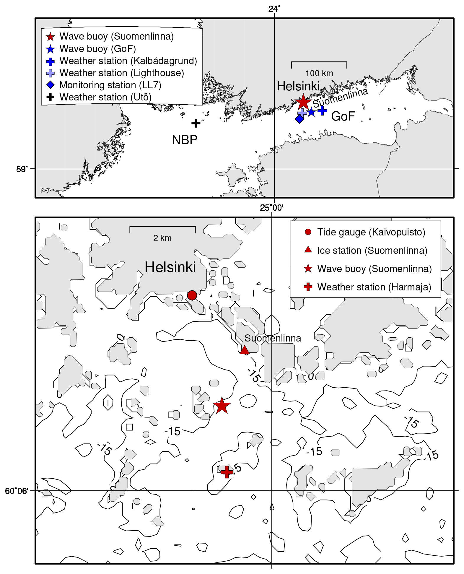
Figure 1 On top is a larger view of the study area covering the Northern Baltic Proper (NBP) and Gulf of Finland (GoF). The coastal area off Helsinki around Suomenlinna is shown on the bottom. The Suomenlinna ice station represents the ice conditions for a radius of about 1 km. The contours show the water depth in metres.

On time scales longer than a week the Baltic Sea water volume variations are a result of the water exchange that is low-pass filtered by the Danish Straits. This water level component is significant, with local sea level variations being up to 1.3 m (Leppäranta and Myrberg, 2009), while precipitation, evaporation, and river runoff play a minor role. On even longer time scales, the Baltic Sea is affected by the global mean sea level rise, which is counterbalanced to a varying extent by the local post-glacial land uplift (e.g. Pellikka et al., 2018; Vestøl et al., 2019).

The wind-generated waves in the GoF are influenced by the fetch, the seabed, and the narrowness of the gulf (Kahma and Pettersson, 1994). The measured significant wave height has exceeded 5 m both during easterly and westerly winds (Pettersson et al., 2013; Pettersson and Jönsson, 2005), but the significant wave height close to Helsinki is expected to be less than half of the open-sea value, since waves are effectively attenuated by the coastal archipelago (Björkqvist et al., 2019).

Finally, both the sea level variations and the waves are affected by the ice season, which in the Baltic Sea is 5–7 months (Leppäranta and Myrberg, 2009). While the presence of ice somewhat attenuates sea level variability – mainly by blocking the piling-up effect of wind on the sea surface (Lisitzin, 1957) – it completely blocks waves if the ice concentration is high enough. The maximum ice coverage ranges from 12.5 % to 100 % of the surface area of the Baltic Sea (Leppäranta and Myrberg, 2009); in normal and severe ice winters, the entire GoF becomes ice covered, while in mild winters only the eastern part of the gulf freezes.

In this paper, we explore the correlation of sea level and wind waves near Helsinki on the northern coast of the GoF, with the aim of determining its effect on the exceedance frequencies of their sum. The study is motivated by the high relevance of flood risk estimates for the City of Helsinki, as well as the recently obtained 4-year time series of coastal wave buoy data. These data, together with the multi-decadal time series of tide gauge observations, provide an excellent data set for such case study. We aim at answering the following research questions:

1. To what extent are these two variables correlated, and does it depend on season, ice conditions, or wind direction?

2. What is the observation-based probability distribution of the sum of the still water level and wave height? How much does it differ from a distribution formed assuming that the two variables are independent?

3. Can a copula-based bivariate distribution account for the correlation of the two variables, and more accurately describe the probability of the sum?

This paper is structured as follows. In Sect. 2, we describe the observation data sets used, the parametric wave model, and the methods used in calculating the uni- and bivariate probability distributions. The results are presented in Sect. 3, followed by a discussion in Sect. 4. We summarize our conclusions in Sect. 5.

2 Data and methods

2.1 Sea level measurements

Automated tide gauges have been operational on the Finnish coast since the late 19th century, at Helsinki since 1904 (see e.g. Johansson et al., 2001 for a more detailed description of data, measurement techniques, and quality). We used instant hourly sea levels measured during 1992–2019 at the Helsinki Kaivopuisto tide gauge (Fig. 1), currently operated by the Finnish Meteorological Institute (FMI). Missing values were estimated by linear interpolation from the measurements at two other nearby tide gauges on the Finnish coast (Hanko and Hamina). There were 477 interpolated hourly values during 1992–2019, less than 0.2 % of the data. All sea levels in this study are given in relation to the N2000 height system, a Finnish realization of the common European height system (Saaranen et al., 2009).

The average sea level during 1992–2019 at Helsinki was +0.21 m, with variations ranging from −0.73 to +1.69 m (Table 1). The linear trend in the time series was −2 cm in 28 years – the land uplift and sea level rise practically cancelling each other. These long-term phenomena thus have a negligible contribution to the sea level variations studied here.

2.2 Wind and temperature measurements

FMI's automatic weather stations provided wind speed, wind direction, and air temperature measurements (Fig. 1), which were used as a forcing for the parametric wave model (Sect. 2.4). From 1992 onwards these stations covered three areas of the Baltic Sea: (i) Northern Baltic Proper (NBP) covered by Utö weather station (measuring height 19 m a.m.s.l. (metres above mean sea level)), (ii) GoF covered by Kalbådagrund and the Helsinki Lighthouse (31 and 33 m a.m.s.l.), and (iii) the coastal area near Suomenlinna, Helsinki covered by Harmaja (18 m a.m.s.l.). The Helsinki Lighthouse weather station was only used for 2019 to cover a Kalbådagrund data gap.

We calculated hourly wind and air temperature values by either interpolating the older 3 h data (up until mid- to late 1990s) or by calculating hourly averages of later denser measurements. All gaps shorter than 6 h were interpolated. Continuous data blocks that were shorter than 12 h were removed. Sea surface temperature (SST) data were only available from Harmaja starting at the end of June 1995. For other times and locations we estimated the SST using a mean yearly cycle from the GoF monitoring station LL7 (Fig. 1). The mean is defined from 434 CTD soundings from R/V Aranda between 1992 and 2017.

2.3 Observed wave heights

FMI's operational GoF wave buoy is located in the centre of the basin (62 m water depth), while the coastal wave buoy is anchored at a depth of 22 m outside of Suomenlinna, Helsinki (Fig. 1). While coastal wave measurements have been made in several places along the Finnish coast, this is the only permanent coastal wave buoy. Yearly measurements at these locations started in 2000 (GoF) and 2016 (Suomenlinna). In the Baltic Sea wave buoys are removed before the ice season, since freezing damages the sensors of the Datawell Directional Waveriders. The GoF buoy's measurement periods were 1–18 January 2016, 12 March 2016–13 January 2017, 18 April 2017–29 January 2018, 14 April 2018–14 January 2019, and 11 March–31 December 2019. For the Suomenlinna wave buoy they were 27 April–29 November 2016, 20 April–15 December 2017, 3 May–26 November 2018, and 18 April–10 December 2019.

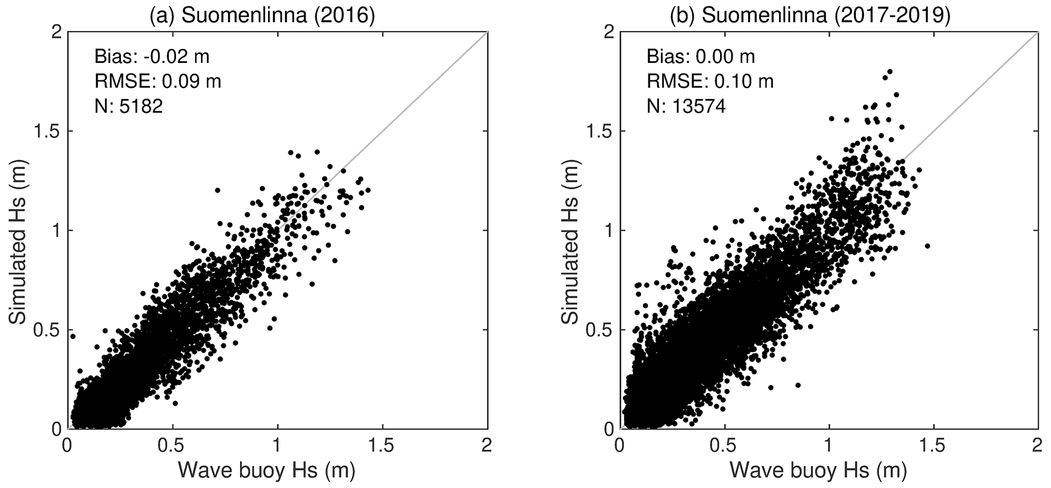
Figure 2 The significant wave height simulated by the parametric wave model compared with observations from the Suomenlinna wave buoys. The (a) 2016 data used for model calibration and (b) the 2017–2019 data are shown separately.

The wave buoys determined the significant wave height from 27 min vertical displacement time series as $H_{\mathrm{s}}=\mathrm{4}\sqrt{m_{\mathrm{0}}}$, where m₀ is the zeroth moment of the variance density spectrum (see Datawell, 2019). We picked every other value to get a data set with hourly time resolution. Of these values, the highest significant wave heights during 2016–2019 were 4.12 m (GoF) and 1.47 m (Suomenlinna); the mean values were 0.81 and 0.33 m.

2.4 Simulated wave heights

We complemented the coastal wave measurements at Suomenlinna with 28 years (1992–2019) of simulations produced by a parametric wave model. The model uses fetch-limited wave growth relations (Kahma and Calkoen, 1992), while also accounting for the wind duration and the atmospheric stratification. A description of the wave evolution scheme is presented in Appendix A.

First we simulated the wave conditions at the GoF wave buoy, which were needed as boundary conditions for the coastal wave hindcast. The GoF simulation accounted for the locally generated waves in the middle of the gulf and waves propagating from the eastern part of the basin and the NBP – also simulated using the same model and the local wind. We then determined the fraction of the GoF wave energy that arrived to Suomenlinna; these waves have longer periods than what can be generated by the local wind and the nearest fetch, and will henceforth be called “long waves”. This long wave energy was quantified as the difference between the observed wave energy (for 2016) and the modelled local wave energy at Suomenlinna. The attenuation – as a function of the wind direction – was determined using a linear regression between the simulated wave energy at the GoF and the estimated long wave energy at Suomenlinna. The final time series of coastal significant wave height was determined from the sum of the simulated local wave energy at Suomenlinna and the attenuated GoF wave energy.

The simulated significant wave heights were validated using wave buoy data from 2016 to 2019. At GoF the −0.02 m bias and 0.28 m RMSE (N=25 293) were slightly worse than for state-of-the-art numerical wave models (e.g. Tuomi et al., 2011; Björkqvist et al., 2018). Nonetheless, the accuracy was sufficient to serve as boundary conditions for the coastal simulations at Suomenlinna, which had a 0.00 m bias and 0.10 m RMSE (N=13 574) (Fig. 2). For Suomenlinna the validation statistics compare well with those from high-resolution numerical wave model simulations (Björkqvist et al., 2020), but the parametric model showed a slight tendency to overestimate the highest significant wave heights (Fig. 2b). This is natural, since a linear regression cannot account for the increased wave–bottom interaction for the higher and longer waves during stronger winds that were not captured in the calibration period. We can, however, conclude that the quality of the simulated wave height time series is adequate for the purpose of this study.

2.5 Ice conditions and wave statistics types

Data originating from FMI's ice charts described the ice conditions at the southern point of the Suomenlinna islands (Fig. 1). The data represent an area with a radius of roughly 1 km and are therefore fairly representative of the wave buoy location. Of the statistics available for the entire study period (1992–2019), we used the start and end dates of the permanent ice-cover. During this time – defined as our ice period – the ice concentration is typically high (over 80 %), making it reasonable to set the significant wave height to zero. The length of our ice period varied from zero (winters 2007–2008, 2017–2018, and 2018–2019) to 139 d (winter 2002–2003).

Table 1 The sea level (still water level, z_still) and significant wave height (H_s) data sets used in this study.

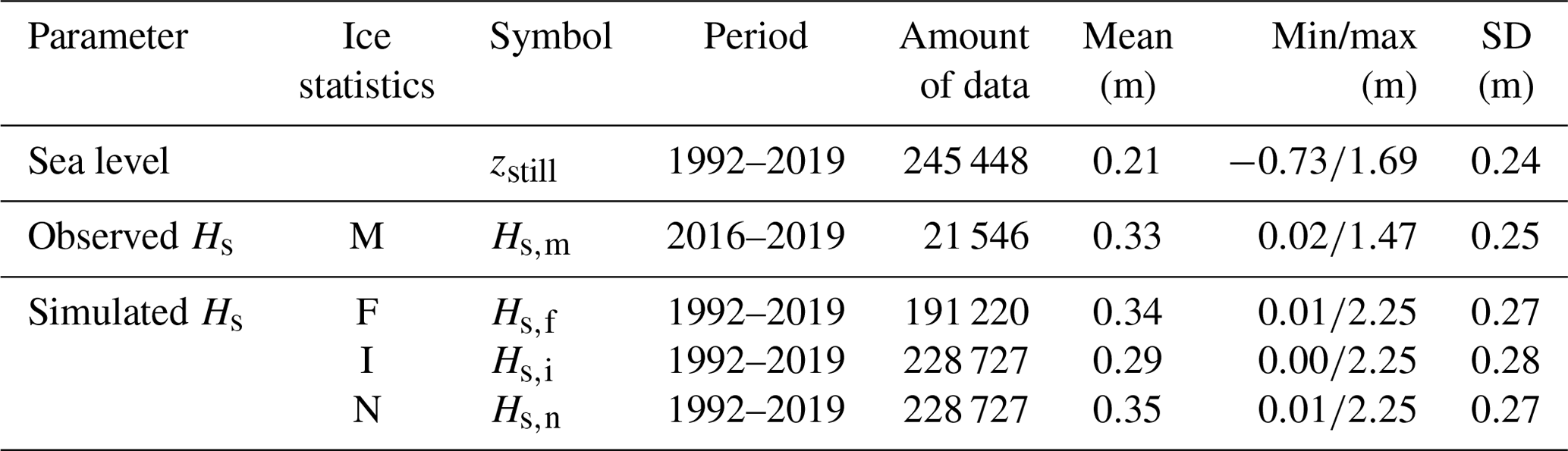
Tuomi et al. (2011) defined four different wave statistics for water bodies with a seasonal ice cover. Using this classification, we compiled the following data sets (Table 1):

• Data set F (ice-free time): simulated H_s for the open water season only.

• Data set I (ice-time-included): simulated H_s set to 0 for the ice period.

• Data set N (hypothetical no-ice): full simulated H_s data set. As the wave model does not account for ice, this represents a hypothetical situation with no ice present.

• Data set M (measurement statistics): wave observations only (this time is a true subset of the ice-free period because of measurement gaps).

We divided the 28-year data sets (F, I, and N) into seven consecutive 4-year periods, from 1992–1995 to 2016–2019. These 4-year time series were, where applicable, used to study temporal variability.

2.6 Probability distribution of the total water level

We defined the total water level, z_max, as the hourly maximum level to which the continuous water mass reaches as a combined effect of the still water level, z_still, and the wave action. To do this, we first assumed that z_still does not change during 1 h. Neglecting site-specific coastal effects, z_max in such case is determined by the highest individual wave crest, η_max. (Note that wave crest denotes the height above z_still, thus being half of the actual height of the highest wave.) At Suomenlinna the highest single wave crest during 30 min is approximately 92 % of the significant wave height (Björkqvist et al., 2019), which we rounded up to η_max=H_s for hourly values. With these assumptions, the maximum water level elevation is

$$\begin{array}{}\text{(1)}& z_{\max }=z_{\mathrm{still}}+{\mathit{\eta }}_{\max }=z_{\mathrm{still}}+H_{\mathrm{s}}.\end{array}$$

The probability distributions of z_max were then calculated directly from the time series obtained from the observed and simulated z_still and H_s data. The distributions of z_still and H_s both describe the actual duration of the phenomenon, and thus have units of h yr⁻¹. The distribution of z_max, on the other hand, has a unit of events per year, where “event” is defined as the instant hourly maximum total water level.

If simultaneous time series of z_still and H_s are not available, the cumulative distribution function (CDF) of z_max needs to be calculated based on the respective univariate distributions. If the two variables are assumed to be independent (for dependent variables, see Sect. 2.7), the CDF of their sum is the convolution

$$\begin{array}{}\text{(2)}& F_z\left(z_{\max }\right)=\underset{\mathbb{R}}{\int }{f}_x\left(\mathit{\xi }\right)F_y\left(z_{\max }-\mathit{\xi }\right)\mathrm{d}\mathit{\xi },\end{array}$$

where f_x denotes the probability density function (PDF) of z_still, and F_y denotes the CDF of H_s (see Leijala et al., 2018 for more details).

2.7 Copula-based probability distributions

Sklar's theorem (Nelsen, 2006) states that if H is a bivariate CDF with marginal CDFs F₁ and F₂, then a copula C exists such that

$$\begin{array}{}\text{(3)}& H\left(x_{\mathrm{1}},x_{\mathrm{2}}\right)=C\left(F_{\mathrm{1}}\left(x_{\mathrm{1}}\right),F_{\mathrm{2}}\left(x_{\mathrm{2}}\right)\right).\end{array}$$

Thus, the joint distribution H can be expressed as a function of the marginal distributions F₁ and F₂ and the copula C, which describes the dependency of the variables x₁ and x₂. If x₁ and x₂ are independent, the copula is simply the product F₁(x₁)F₂(x₂). An extensive introduction to copula methods is provided by Genest and Favre (2007). A benefit of the method is that the marginal distributions can be of any form.

We studied the suitability of nine different copulas (Gumbel, Frank, Clayton, Normal, t-EV, Hüsler–Reiss, Galambos, Tawn, and Plackett) in representing the dependence structure of the observed z_still and H_s data (2016–2019). We calculated the parameters for each copula with the inversion of Kendall's τ estimator. To quantify the goodness-of-fit for each of these copulas, we calculated the Cramér–von Mises statistic S_n as defined in Eq. (2) of Genest et al. (2009).

By using the bivariate distributions consisting of each of the nine copulas and the marginal distributions (Sect. 2.8), we simulated 10⁸ random pairs (z_still, H_s) and calculated the complementary cumulative distribution functions (CCDFs) of their sum. The calculations were performed with the R package “copula: Multivariate Dependence with Copulas” (Hofert et al., 2020; Yan, 2007; Kojadinovic and Yan, 2010; Hofert and Mächler, 2011).

2.8 Marginal distributions and extrapolation

Probabilities of sea level extremes have been estimated using extreme value distributions with, e.g. block maxima (annual/monthly) or peak-over-threshold values (e.g. Arns et al., 2013). However, when the focus is on the sum of sea level and wave height (Eq. 1), it is essential to use simultaneous values, and the extremes generally do not co-occur. Our aim was to study the correlation between these two variables in general, on a hourly time scale, not just the correlation of extremes. Thus, we chose to base our analysis on the entire data set of hourly values.

Our 28 years of hourly data allow for a direct estimate of the exceedance frequency down to 0.036 h yr⁻¹, and we therefore had to extrapolate the distribution to cover rarer values. Extremes are typically evaluated using some extreme value distribution (Eelsalu et al., 2014; Särkkä et al., 2017; Kulikov and Medvedev, 2017), but this approach is not applicable to extrapolate hourly data needed for this study.

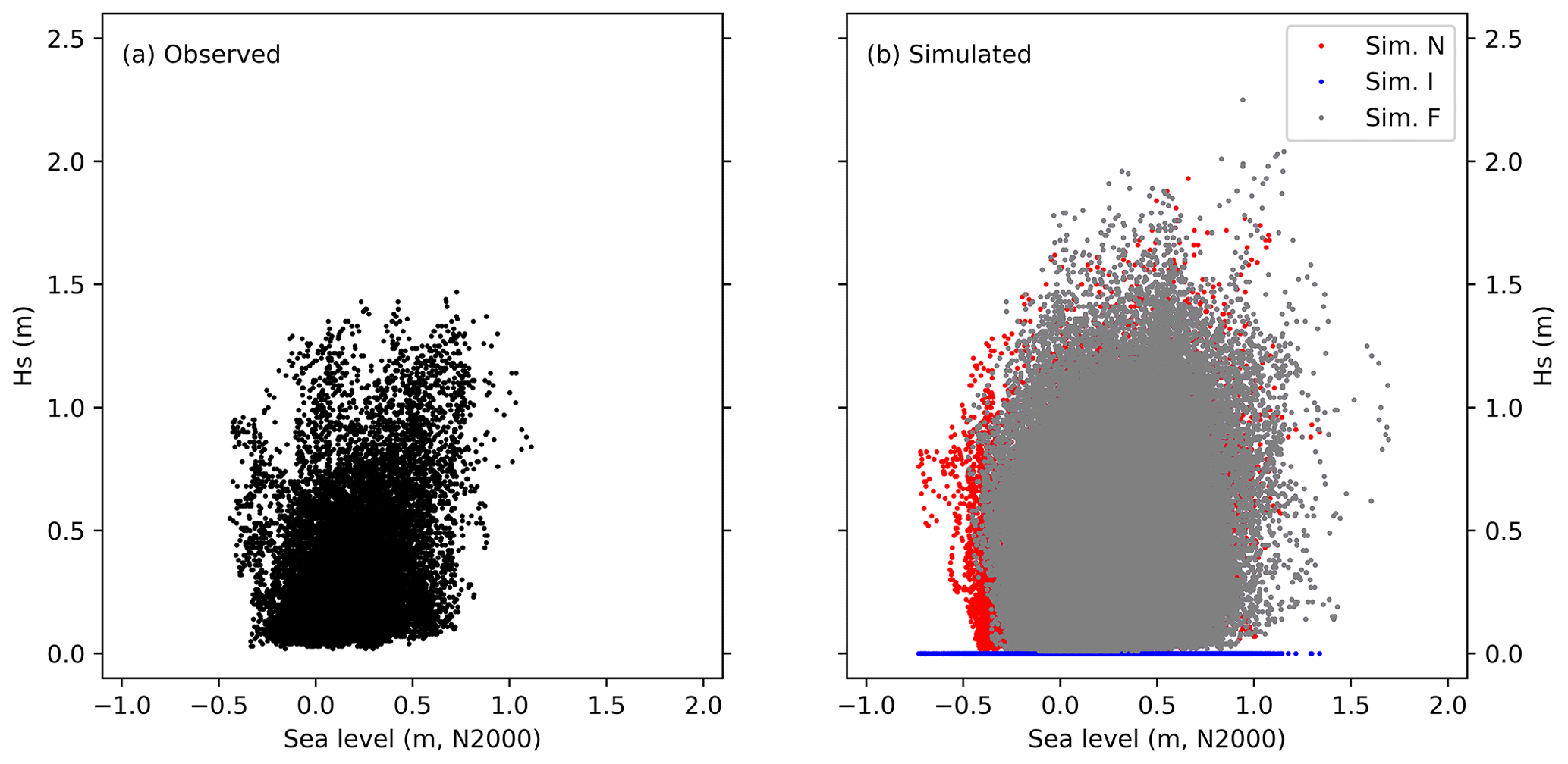
Figure 3 Scatter plot of significant wave heights vs sea level: (a) observed wave heights from 2016 to 2019 and (b) simulated wave heights from 1992 to 2019, data sets F (grey), I (blue), and N (red). Note that every data point of the set F (ice-free time) is also included in sets I (wave height set to zero during ice-covered time) and N (hypothetical no-ice wave heights).

The probability distribution of the observed sea levels on the Baltic Sea coasts is slightly asymmetric: the high-end tail is thicker than the low-end tail (e.g. Johansson et al., 2001; Kulikov and Medvedev, 2017). The significant wave heights in the archipelago, again, show a clear tendency to saturate (Leijala et al., 2018), and are therefore not modelled well simply by applying some commonly used distribution type, such as the Weibull distribution (e.g. Battjes, 1972; Mathisen and Bitner-Gregersen, 1990). We used the empirical frequency distributions for exceedance frequencies between the 0.5 and 99.5 percentiles, which correspond to a frequency of 44 h yr⁻¹ in the tail of the CDF/CCDF. We extrapolated the high (low) tails of the distribution by fitting two-parameter exponential functions $F=e^{-\mathit{\lambda }\left(x-x_{\mathrm{0}}\right)}$ to the CCDFs (CDFs) below this frequency, following, e.g. Leijala et al. (2018). This method was applied consistently to the sea level, significant wave height (only high tail), and total water level data. The PDFs were obtained by numerically differentiating the CDFs. As our main focus in this study is not on the extrapolated extreme ends of the distribution, we left more detailed considerations of the extrapolation function out and considered the simple exponential function sufficient for our purposes.

3 Results

3.1 Correlation

The simultaneous hourly sea levels and significant wave heights (Fig. 3) indicate some positive tail dependence – high sea levels co-occurring with high waves – both in the observed and simulated data. However, high waves also occur with moderate or even low sea levels, and high sea levels are not necessarily accompanied by high waves either. The individual maxima did not occur simultaneously. During the highest measured sea level (1.69 m) on 9 January 2005, the simulated wave height was a relatively modest 0.87 m. The highest observed wave height was 1.47 m on 7 December 2017, while the simulations gave 2.25 m on 23 December 2004. On those occasions, the sea levels were +0.73 and +0.94 m, respectively: high but not extreme.

The variations in both parameters are largest in winter (DJF; Fig. 4) and smallest in summer (JJA), when the wave height did not exceed 1.5 m and the sea level was between −0.3 and +1.0 m. The positive tail dependence can be seen in most of the seasonal data also.

The hypothetical no-ice data (type N) show situations with low sea level and wave heights ranging from 0 to 1 m, which would have occurred during the ice-covered period, especially in DJF (Figs. 3 and 4). In spring (MAM), also many high-sea-level and hypothetically high-wave situations occurred during the ice-covered time.

Figure 4 Scatter plots of (a) winter, (b) spring, (c) summer, and (d) autumn events. Black: observed wave heights from 2016 to 2019. Other colours: simulated wave heights from 1992 to 2019; ice types F (grey), I (blue), and N (red).

As a measure of the correlation, we used Kendall's tau coefficient (τ). It measures rank correlation: the similarity of the orderings of the data when ranked by each of the quantities. Thus, no assumption of a linear relationship between the variables is made. The sea level correlates stronger with the observed wave heights than the simulated wave heights from the same period (the measurement seasons during 2016–2019) on all seasons except DJF (Table 2). The observed wave data in DJF are very sparse (Fig. 4a), practically only consisting of 15 d of observations in December 2017 and 10 d in December 2019, and thus the high correlation (τ=0.3) should not be considered representative. Likewise, the observations for MAM only represent late April and May, as the earliest the wave buoy was deployed was on 18 April and the latest on 3 May. Of the different seasons, autumn (SON) shows the lowest correlation in all data sets.

Table 2 Kendall rank correlation coefficients (τ) between the observed (Obs.) and simulated (Sim.) significant wave heights and sea levels in four seasons: winter (DJF), spring (MAM), summer (JJA), and autumn (SON). The data set “Sim. M” includes the simulated significant wave heights from the same periods as the data set “Obs. M” contains observations, thus being a subset of “Sim. F” of the years 2016–2019.

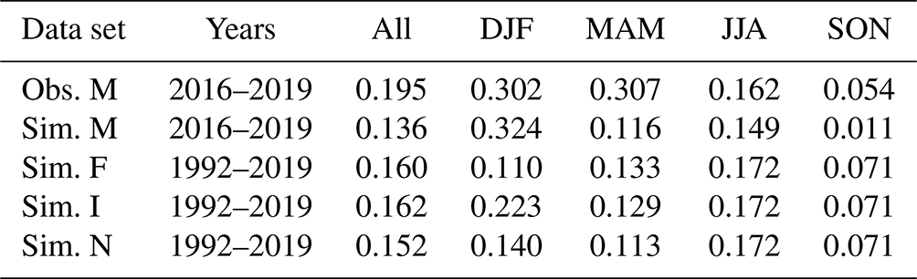
The different ways of handling the ice time in the 28-year data sets (F, I, N) do not generally result in large differences in the correlation, the only exception being DJF where the data set I shows clearly higher correlation than data sets F or N. There is a tendency for lower sea levels during the ice-covered period (the blue points with H_s=0 in Fig. 4a), which likely enhances the correlation.

The correlation clearly depends on wind direction measured at Harmaja (Fig. 5, nautical convention for wind direction). The strongest positive correlation occurs with southwesterly winds (240–260^∘), while northeasterly winds (20–50^∘) result in zero or negative correlation. The behaviour is qualitatively similar in both the observed and simulated wave heights, and with all the data sets considered (F, I and N; results for data sets I and N shown in Appendix B).

Figure 5 The Kendall correlation coefficients (τ) between significant wave height and sea level for different wind directions. The blue dots show correlation in 1^∘ direction bins, and the red dots in 10^∘ bins. The significant wave heights from (a) buoy observations during 2016–2019 and (b) simulated data set F during 1992–2019 are shown. The direction given is the direction from where the wind blows (nautical convention), observed at Harmaja weather station. The correlation coefficients for all data (τ=0.20 and 0.16; Table 2) are shown as horizontal lines.

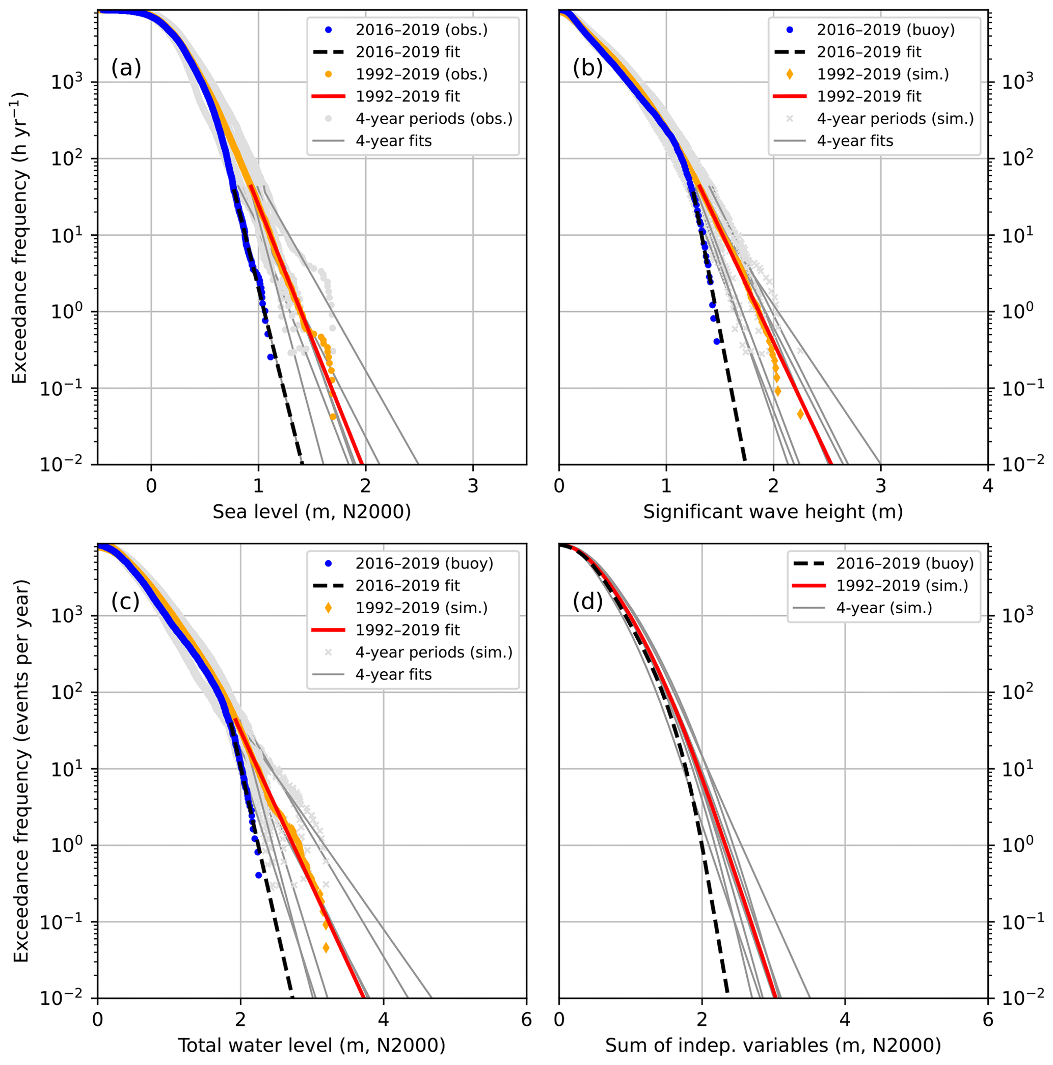
Figure 6 The CCDFs of (a) observed hourly sea levels, (b) observed/simulated significant wave heights, (c) total water level as their sum, and (d) total water level calculated as a sum of two independent variables. The distributions shown are those for the data set F (ice-free season). The distributions were extrapolated with exponential functions below the exceedance frequency of 44 h yr⁻¹. The seven consecutive 4-year periods shown separately for observed sea levels and simulated waves are 1992–1995 to 2016–2019.

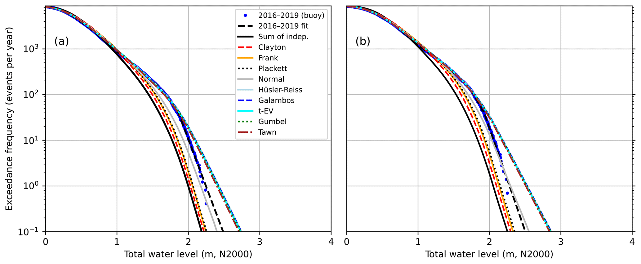
Figure 7 The observation-based CCDF of total water level during 2016–2019 (“buoy” + “fit”), the CCDF calculated assuming the variables independent (“Sum of indep.”), as well as CCDFs calculated by taking 10⁸ random samples based on the nine different copulas combined with the observation-based marginal distributions for (a) all data and (b) situations with southwesterly wind (160–340^∘).

3.2 Probability distributions

The CCDF of the sea level from the period 2016–2019 shows lower frequencies for high sea levels (>0.7 m) than the CCDF from the entire period 1992–2019 (Fig. 6a). The 2016–2019 distribution is also on the lower limit of the ensemble of the seven different 4-year distributions. The period 2016–2019 had less high sea levels than most of the 4-year periods, having also the lowest 4-year maximum (1.11 m) of all these periods. The distribution from 2004 to 2007 has a distinct tail with sea levels exceeding 1.45 m, while the maxima of all the other periods are below this. All these high values resulted from the exceptional storm Gudrun on 9 January 2005, when the sea level at Helsinki stayed above 1.4 m for 13 h from 01:00 to 13:00 UTC.

The shape of the CCDF obtained from the observed wave heights differs from those obtained from the simulated wave heights (Fig. 6b), the exceedance frequency decreasing more rapidly with increasing wave height in the observed CCDF than in the simulated ones. This is in accordance with the parametric wave model validation (Fig. 2b), which showed an overestimation of the highest significant wave heights.

The CCDFs of z_max calculated by summing the observed sea levels and observed or simulated wave heights according to Eq. (1), and extrapolating with exponential functions, show similar behaviour (Fig. 6c): The distribution based on observed wave heights shows lower frequencies for high z_max (>2.0 m) than any of those based on simulated wave heights. The distributions of the sum of z_still and H_s obtained by assuming the two variables independent, according to Eq. (2) (Fig. 6d) give lower probabilities for high z_max than the distributions of Fig. 6c. Below the exceedance frequency of 100 events per year down to 0.1 events per year, the assumption of independence leads to an underestimation of 0.2–0.3 m in z_max of the observed distribution from 2016 to 2019. In the simulated 4-year distributions, the underestimation at 100 events per year ranges from 0.15 to 0.28 m, and at 1 event per year from 0.09 to 0.70 m. In the distribution based on the entire 28-year simulation, the underestimation increases with decreasing exceedance frequency, from 0.06 m at 1000 events per year to 0.55 m at 0.1 events per year.

The CCDFs based on data sets F, I, and N show only minor differences (Fig. 6 for F, others in Appendix B). This indicates that the hypothetical wave and sea level behaviour during the ice-covered time does not differ from that during the open water period. The number of ice days, however, is small compared to the length of the study period: 28 d (1.9 %) during 2016–2019 and 1615 d (16 %) during 1992–2019. Thus, it is expected that they do not significantly alter the results.

3.3 Copula-based distributions

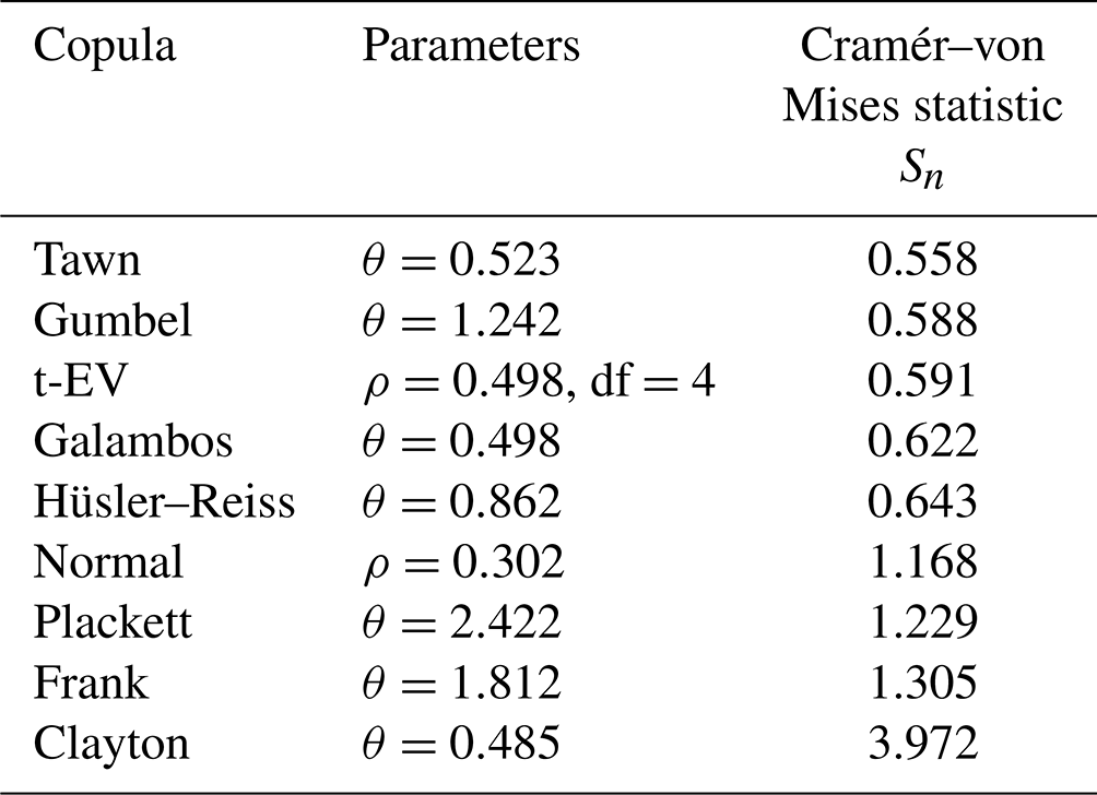
Table 3 shows the parameters of the different copulas fitted to the sea levels and significant wave heights. In Fig. 7, CCDFs obtained from these copulas and the marginal distributions are compared with the observed CCDF and the CCDF obtained by assuming the two variables independent. In accordance with the above results, the observed CCDF shows higher probabilities of high total water levels (>1.1 m) than the independent case (Eq. 2).

The copulas are divided into two distinct groups. The Clayton, Frank, and Plackett copulas remain close to the independent case. On the other hand, Tawn, Gumbel, t-EV, Galambos, and Hüsler–Reiss copulas capture more of the effect of dependence on the distribution, closely following the observed distribution down to exceedance frequency of 50 events per year. The Normal copula falls between these two groups, deviating from the observed distribution below 400 events per year. This behaviour is confirmed by the Cramér–von Mises statistics (Table 3), where smaller S_n values correspond to better fit. For the latter group S_n<1, while in the first group S_n varies from 1.22 to 3.97. The Normal copula, again, falls between these groups with S_n=1.17.

Table 3 Fitted parameters of nine different copulas for sea levels and significant wave heights from buoy observations for the period 2016–2019.

We tested the effect of wind direction on the copula results by conducting the copula analysis separately for two subsets of the data: situations with southwesterly wind (160–340^∘, Fig. 7b) and northeasterly wind (340–160^∘, not shown). The results for the southwesterly wind subset are qualitatively similar to those including all data: Copulas are divided into two groups. The stronger correlation (τ=0.269) results in somewhat higher probabilities of high total water levels in the distributions. In the northeasterly wind case, on the other hand, the non-existent correlation ($\mathit{\tau }=-\mathrm{0.012}$) leads to the copula analysis being somewhat pointless, as all the copulas end up close to the independent case.

To further illustrate the differences in bivariate distributions based on different copulas, we simulated an ensemble of 21 546 samples from each, these being of the same size as the observed data set (Fig. 8). The copulas with S_n<1 (Tawn, Gumbel, t-EV, Galambos, and Hüsler–Reiss) tend to show a positive tail dependence: the slight bending of the scatter cloud into a tail on the upper right corner. The copulas with S_n>1 do not show such an apparent positive tail.

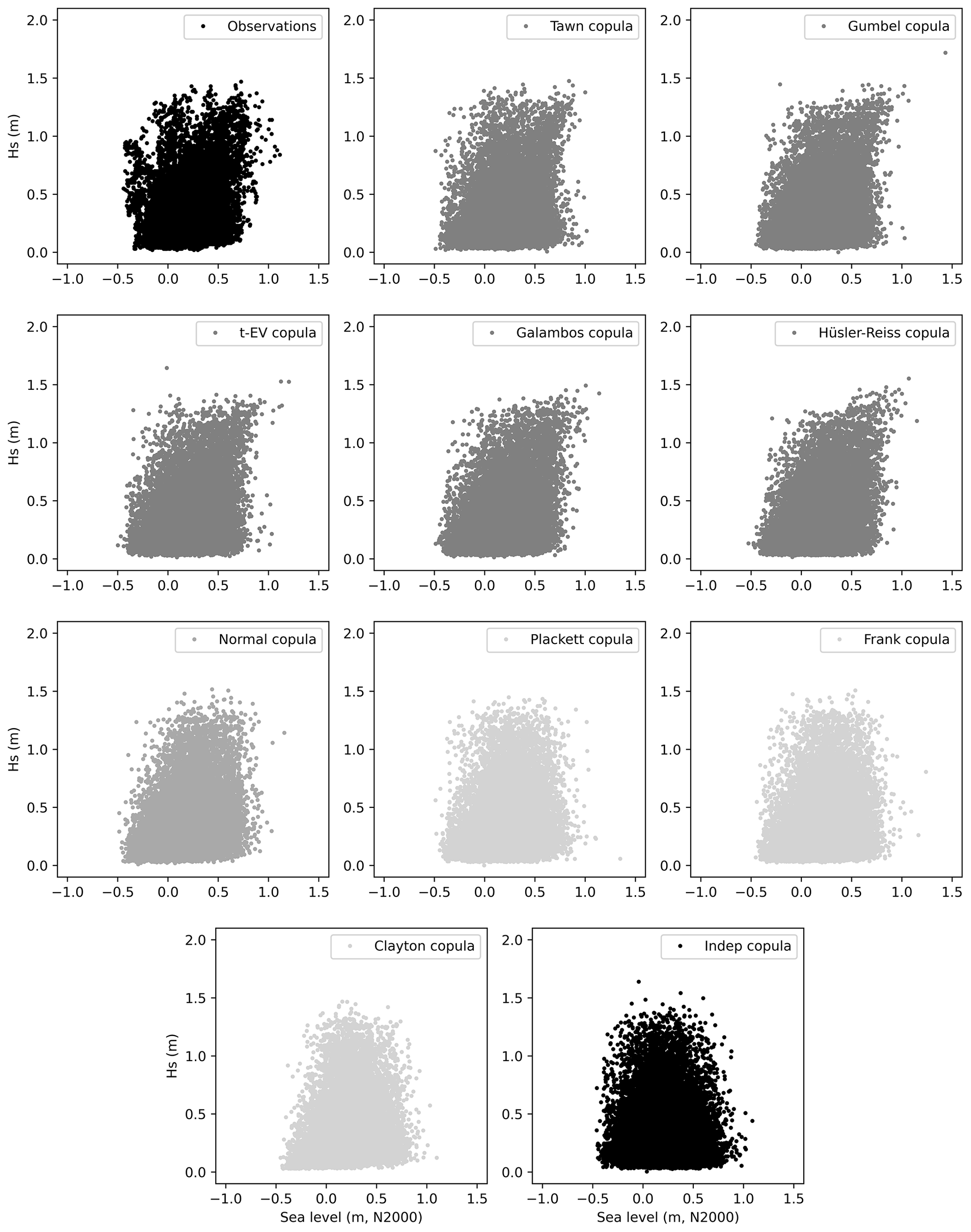
Figure 8 Scatter plots of the observed sea level (z_still) and significant wave height (H_s) during 2016–2019 (top left), and scatters of 21 546 random points (equalling the count of observations) sampled from the bivariate distributions based on the nine different copulas and the independence copula.

4 Discussion

Since the wave conditions in the archipelago markedly differ from those on the open sea, a multi-year time series of wave data from a coastal location such as Suomenlinna provides excellent material for studies. As more data accumulate, it will provide more comprehensive knowledge on the local wave behaviour. We compensated for the shortness of the wave buoy time series by using 28 years of simulated wave data. The lightweight parametric wave model is considerably faster to run than high-resolution numerical wave models. Nevertheless, the bias and RMSE of the simulations were comparable.

The validation suggested that the highest wave heights are overestimated in the simulations. The attenuation of longer waves through bottom processes is indirectly accounted for in the model through the calibration against measurements. Nonetheless, this calibration might not hold for even harsher weather conditions and even longer waves. While the simulations offer a good tool for assessing the general dependence between the wave height and sea level variations, they should not be used as is for analysing extreme values. If the wave simulations of the parametric model are to be used for extreme conditions, the wave-bottom interactions need to be accounted for in a more explicit manner, and such improved model needs to be re-validated.

One of the advantages of a wave model is its ability to simulate the wave conditions during ice-covered periods, or periods when there is a risk of freezing and the wave buoy cannot be kept in the sea. This extends the time series and provides an opportunity to analyse the question, “What would happen if there was no ice?” This question is relevant when we consider the conditions in the GoF in a warmer future climate, for instance. Our results did not indicate that the wave or sea level conditions, or the correlation of these, would markedly differ from those occurring during the ice-free period in the present climate.

The wave conditions vary significantly among 4-year periods (Fig. 6). The observational period of this study (2016–2019) was relatively calm: the 4-year maximum sea level (1.11 m) was lowest among the seven consecutive 4-year sets, while the maximum simulated significant wave height (1.89 m) ranked fourth. To obtain reliable estimates for probabilities of extreme sea levels on the Finnish coast, at least 30 years of data are generally used (e.g. Pellikka et al., 2018; Kahma et al., 2014). Our results obtained from 4-year time series do not provide any flooding risk estimates for practical applications.

Additionally, considering flooding on the coast, the relevant parameter is the wave run-up. While our total water level (Eq. 1) represents the elevation of the highest wave crest on the open sea, it is not applicable on the waves meeting the coastline. On a steep coast, a more appropriate estimate for the total water level would be $z_{\mathrm{still}}+\mathrm{2}\cdot H_{\mathrm{s}}$ due to wave reflection (Leijala et al., 2018), while on a shallow coast the eventual run-up on the coastline is less than z_still+H_s.

The behaviour of the correlation with respect to wind direction (Fig. 5) is readily explained by the geography of the GoF. Southwesterly winds push water into the gulf and simultaneously raise high waves, leading to a positive correlation. Northeasterly winds, on the other hand, push water out from the GoF while still raising waves, which results in a negative correlation. When the correlation is calculated from the entire data set, these two opposing situations with different mechanisms likely cancel each other and reduce the overall correlation. To more completely describe the effect of the correlation on the distribution of the total water level, and thus the flooding risks, one option might be to use three variables instead of two: still water level, significant wave height, and wind direction. We leave this as an option for future studies.

The sea level processes in the GoF act on different time scales, from the sub-daily storm surges to sub-weekly Baltic Sea internal variations, and weekly and longer-term changes in the total water volume. From 1 d to 1 week, the Baltic Sea mainly responds to wind and air pressure forcing like a closed basin. The response time of such variations, e.g. the transport of water between the GoF and the Baltic Proper in a seiche oscillation, is usually of the order of 1 d. In such time scale, the wind-generated waves have time to develop, and these phenomena co-occur.

The sea level variations in time scales longer than 1 week usually involve changes in the Baltic Sea water volume. These are related to longer-term (up to 60 d; Särkkä et al., 2017) prevailing wind conditions, which control the in- or outflow of water in the Danish Straits. These should not have a direct relationship with the local waves. However, the longer-term weather conditions correlate with short-term weather phenomena too: e.g. prevailing westerly winds are related to more low-pressure systems with strong winds travelling over the Baltic Sea, and might thus contribute to the overall correlation.

Our results demonstrated that the assumption of independence of sea level and significant wave height leads to an underestimation of total water levels with exceedance frequencies of 100 events per year or less by about 0.2–0.3 m in the 4-year observation-based data set, and up to 0.55 m in the 28-year simulation-based data set (the difference of the distributions in Fig. 6c and d). The underestimation generally increases with lower exceedance frequencies. Since low exceedance frequencies such as 0.001–0.01 events per year are highly relevant for flooding risk considerations, further investigation of the effect of the correlation on such exceedance frequencies would be worthwhile. Quantification of this effect for frequencies that go below our observation/simulation-based data sets, however, would require a more thorough analysis of the suitability of the extrapolation function, which we leave for future studies.

5 Conclusions

Our main conclusions, related to the research questions presented in Sect. 1, are as follows.

The sea level variations and significant wave heights show a positive correlation in general (τ=0.20). The correlation depends on wind direction: Southwesterly winds lead to the strongest positive correlation (up to τ=0.5), while northeasterly winds lead to zero or negative correlation. Ice conditions did not have an apparent effect on the correlation: Including hypothetical no-ice wave heights during the ice season did not markedly alter the correlation, and neither did the setting of the wave height to zero during the ice-covered time.

The 4-year probability distribution of the total water level, calculated as a sum of the observed sea level and observed significant wave heights, gives 0.2–0.3 m higher values for high total water levels (0.1–100 events per year) than the distribution calculated by assuming the two variables independent. In the simulated 28-year distribution, the underestimation amounts to 0.2–0.5 m. As the total water level values rarer than 0.1 events per year are also likely underestimated, the dependence between the variables should be accounted for when calculating the probabilities of high total water levels, e.g. for flooding risk estimates.

The probability distribution of the sum based on the copula approach is closer to the observed distribution than the distribution based on the independence assumption. Of the nine copulas studied, the Tawn, Gumbel, t-EV, Galambos, and Hüsler–Reiss copulas proved most suitable for our data.

Appendix A: Model scheme for wave evolution

The core idea of the wave model is based on known universal properties of different dimensionless parameters, namely the energy, peak frequency, phase speed, fetch, and time:

$$\begin{array}{}\text{(A1)}& {\displaystyle }& {\displaystyle }\stackrel{\mathrm{̃}}{\mathit{\epsilon }}=g^{\mathrm{2}}\mathit{\epsilon }/U^{\mathrm{4}}\text{(A2)}& {\displaystyle }& {\displaystyle }{\stackrel{\mathrm{̃}}{f}}_{\mathrm{p}}=f_{\mathrm{p}}U/g\text{(A3)}& {\displaystyle }& {\displaystyle }{\stackrel{\mathrm{̃}}{c}}_{\mathrm{p}}=c_{\mathrm{p}}/U\text{(A4)}& {\displaystyle }& {\displaystyle }\stackrel{\mathrm{̃}}{X}=gX/U^{\mathrm{2}}\text{(A5)}& {\displaystyle }& {\displaystyle }\stackrel{\mathrm{̃}}{t}=gt/U.\end{array}$$

The wave growth in the model is quantified using the fetch limited wave growth relations of Kahma and Calkoen (1992):

$$\begin{array}{}\text{(A6)}& {\displaystyle }& {\displaystyle }\stackrel{\mathrm{̃}}{\mathit{\epsilon }}=p_{\mathrm{2}}{\stackrel{\mathrm{̃}}{X}}^{p_{\mathrm{1}}}\text{(A7)}& {\displaystyle }& {\displaystyle }{\stackrel{\mathrm{̃}}{f}}_{\mathrm{p}}=q_{\mathrm{2}}{\stackrel{\mathrm{̃}}{X}}^{q_{\mathrm{1}}}.\end{array}$$

The coefficients p₁, p₂, q₁, q₂ for the wave growth relations depend on the atmospheric stratification as presented by the authors.

Instead of assuming that the waves are fetch limited at each time step, the model simulates a more realistic wave growth and decay by also accounting for the limitation of wind duration through the following propagation scheme:

1. Calculate the dimensionless fetch, ${\stackrel{\mathrm{̃}}{X}}_{{\mathit{\epsilon }}^{i-\mathrm{1}}}$, based on the energy from the previous time step, εⁱ⁻¹, and the current wind speed, Uⁱ.

2. Calculate a (dimensionless) duration based on the wind, Uⁱ, and Eq. (A7) as:

   $$\begin{array}{}\text{(A8)}& \begin{array}{rl}{\stackrel{\mathrm{̃}}{t}}_{\mathrm{0}}& =\underset{\mathrm{0}}{\overset{{\stackrel{\mathrm{̃}}{X}}_{{\mathit{\epsilon }}^{i-\mathrm{1}}}}{\int }}{\left({\displaystyle \frac{\mathrm{1}}{\mathrm{2}}}\stackrel{\mathrm{̃}}{c_{\mathrm{p}}}\right)}^{-\mathrm{1}}\mathrm{d}\stackrel{\mathrm{̃}}{X}=\underset{\mathrm{0}}{\overset{{\stackrel{\mathrm{̃}}{X}}_{{\mathit{\epsilon }}^{i-\mathrm{1}}}}{\int }}\mathrm{4}\mathit{\pi }\stackrel{\mathrm{̃}}{f_{\mathrm{p}}}\mathrm{d}\stackrel{\mathrm{̃}}{X},\\ & =\underset{\mathrm{0}}{\overset{{\stackrel{\mathrm{̃}}{X}}_{{\mathit{\epsilon }}^{i-\mathrm{1}}}}{\int }}\mathrm{4}\mathit{\pi }{q}_{\mathrm{2}}{\stackrel{\mathrm{̃}}{X}}^{q_{\mathrm{1}}}\mathrm{d}\stackrel{\mathrm{̃}}{X}={\displaystyle \frac{\mathrm{4}\mathit{\pi }{q}_{\mathrm{2}}}{q_{\mathrm{1}}+\mathrm{1}}}{\stackrel{\mathrm{̃}}{X}}_{{\mathit{\epsilon }}^{i-\mathrm{1}}}^{\left(q_{\mathrm{1}}+\mathrm{1}\right)}.\end{array}\end{array}$$

3. Determine an enhanced dimensionless time step as $\mathrm{\Delta }\stackrel{\mathrm{̃}}{t}+{\stackrel{\mathrm{̃}}{t}}_{\mathrm{0}}$, where Δt is the fixed time step of the model (e.g. 1 h).

4. As an inverse to step 2, calculate a new fetch ${\stackrel{\mathrm{̃}}{X}}_t$ based on the enhanced duration $\mathrm{\Delta }\stackrel{\mathrm{̃}}{t}+{\stackrel{\mathrm{̃}}{t}}_{\mathrm{0}}$, and Eq. (A7) as:

   $$\begin{array}{}\text{(A9)}& {\stackrel{\mathrm{̃}}{X}}_t={\left({\displaystyle \frac{\left(\stackrel{\mathrm{̃}}{t}+{\stackrel{\mathrm{̃}}{t}}_{\mathrm{0}}\right)\left(q_{\mathrm{1}}+\mathrm{1}\right)}{\mathrm{4}\mathit{\pi }{q}_{\mathrm{2}}}}\right)}^{\mathrm{1}/\left(q_{\mathrm{1}}+\mathrm{1}\right)}.\end{array}$$

5. Calculate the minimum dimensionless fetch for a fully developed sea (using the wind speed at 10 m height) as:

   $$\begin{array}{}\text{(A10)}& \begin{array}{rl}{\displaystyle \frac{U}{c_{\mathrm{p}}}}& ={\displaystyle \frac{\mathrm{2}\mathit{\pi }{f}_{\mathrm{p}}U}{g}}=\mathrm{2}\mathit{\pi }{\stackrel{\mathrm{̃}}{f}}_{\mathrm{p}}=\mathrm{0.82}⟺{\stackrel{\mathrm{̃}}{X}}_{\mathrm{FD}}\\ & ={\left({\displaystyle \frac{\mathrm{0.82}}{\mathrm{2}\mathit{\pi }{q}_{\mathrm{2}}}}\right)}^{\mathrm{1}/q_{\mathrm{1}}}.\end{array}\end{array}$$

6. Set the relevant fetch to ${\stackrel{\mathrm{̃}}{X}}^i=\min \mathit{\{}{\stackrel{\mathrm{̃}}{X}}_t,{\stackrel{\mathrm{̃}}{X}}_{\mathrm{FD}},\stackrel{\mathrm{̃}}{X}\mathit{\}}$, where $\stackrel{\mathrm{̃}}{X}$ is the physical dimensionless fetch.

7. Calculate the new energy, εⁱ, and peak frequency, $f_{\mathrm{p}}^i$, using ${\stackrel{\mathrm{̃}}{X}}^i$, Uⁱ, and Eqs. (A6) and (A7).

Appendix B: Supplementary figures

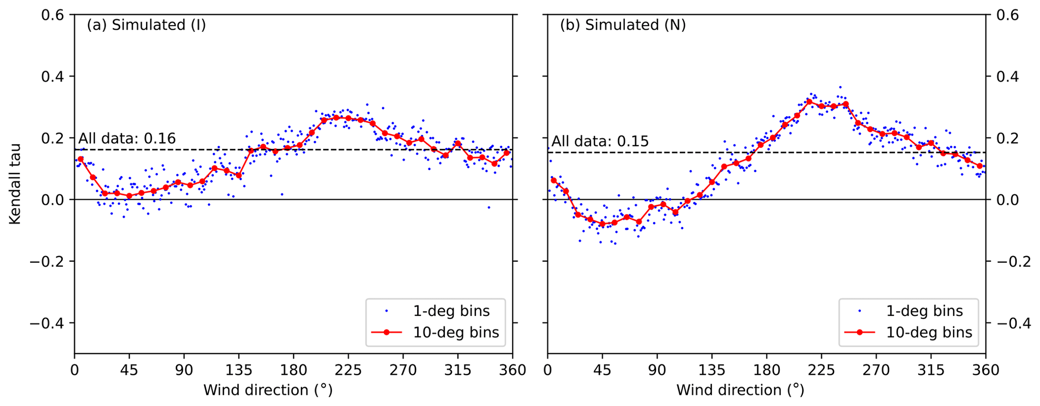
Figure B1 The Kendall correlation coefficients (τ) between significant wave height and sea level for different wind directions. The blue dots show correlation in 1^∘ direction bins, and the red dots in 10^∘ bins. The significant wave heights from simulated data sets (a) I and (b) N 1992–2019 are shown. The direction given is the direction from where the wind blows (nautical convention), observed at Harmaja weather station. The correlation coefficients for all data (τ=0.16 and 0.15) are shown as horizontal lines.

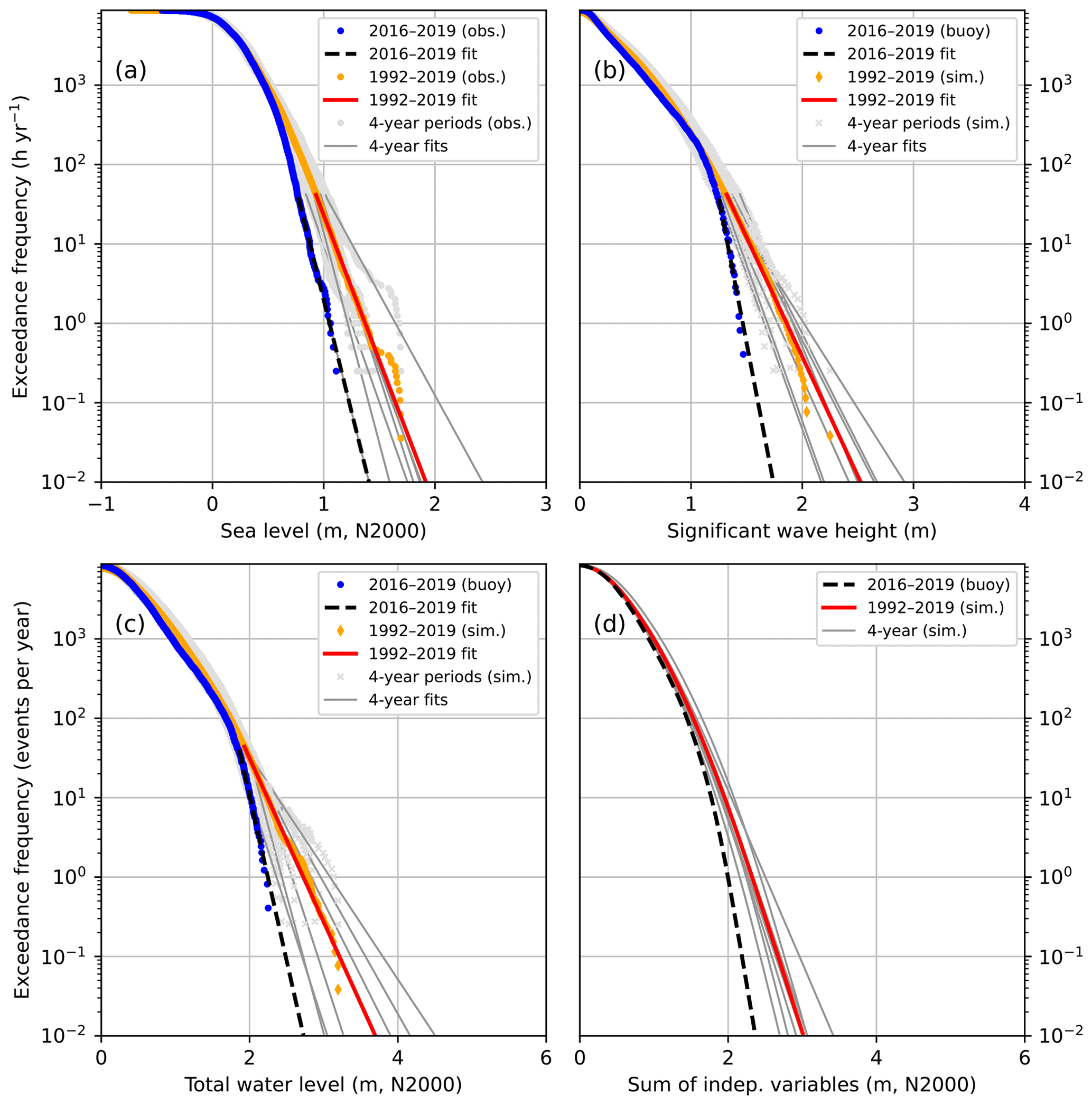
Figure B2 The CCDFs of (a) observed hourly sea levels, (b) observed/simulated significant wave heights, (c) total water level as their sum, and (d) total water level calculated as a sum of two independent variables. The distributions shown are those for the data set N (hypothetical no-ice). The distributions were extrapolated with exponential functions below the exceedance frequency of 44 h yr⁻¹. The seven consecutive 4-year periods shown separately for observed sea levels and simulated waves are 1992–1995 to 2016–2019.

Figure B3 The CCDFs of (a) observed hourly sea levels, (b) observed/simulated significant wave heights, (c) total water level as their sum, and (d) total water level calculated as a sum of two independent variables. The distributions shown are those for the data set I (ice time included). The distributions were extrapolated with exponential functions below the exceedance frequency of 44 h yr⁻¹. The seven consecutive 4-year periods shown separately for observed sea levels and simulated waves are 1992–1995 to 2016–2019.