the Creative Commons Attribution 4.0 License.
the Creative Commons Attribution 4.0 License.
 | 07 Mar 2022
Characteristics of precipitation extremes over the Nordic region: added value of convection-permitting modeling
Emma D. Thomassen
Danijel Belušić
Petter Lind
Peter Berg
Jens H. Christensen
Ole B. Christensen
Andreas Dobler
Erik Kjellström
Jonas Olsson
It is well established that using kilometer scale grid resolution for simulations of weather systems in weather and climate models enhances their realism. This study explores heavy- and extreme-precipitation characteristics over the Nordic region generated by the regional climate model HARMONIE-Climate (HCLIM). Two model setups of HCLIM are used: ERA-Interim-driven HCLIM12 spanning over Europe at 12 km grid spacing with a convection parameterization scheme and HCLIM3 spanning over the Nordic region with 3 km grid spacing and explicitly resolved deep convection. The HCLIM simulations are evaluated against a unique and comprehensive set of gridded and in situ observation datasets for the warm season from April to September regarding their ability to reproduce sub-daily and daily heavy-precipitation statistics across the Nordic region. Both model setups are able to capture the daily heavy-precipitation characteristics in the analyzed region. At the sub-daily scale, HCLIM3 clearly improves the statistics of occurrence of the most intense heavy-precipitation events and the amplitude and timing of the diurnal cycle of these events compared to its forcing of HCLIM12. Extreme value analysis shows that HCLIM3 provides added value in capturing sub-daily return levels compared to HCLIM12, which fails to produce the most extreme events. The results indicate clear benefits of the convection-permitting model in simulating heavy and extreme precipitation in the present-day climate, therefore, offering a motivating way forward to investigate the climate change impacts in the region.
- Article
(5628 KB) - Full-text XML
-
Supplement
(1596 KB) - BibTeX
- EndNote


Precipitation extremes represent a major environmental and socioeconomic hazard worldwide, and the Nordic region is no exception. Notably, locally concentrated intense precipitation can cause flooding in rivers or urban settings, landslides, erosion events, and damages to infrastructure. The three main weather situations producing heavy precipitation within the Nordic region consist of the strong vertical lifting of moist air masses in connection with fronts, within convective cells, or enhanced by orography (Førland et al., 1998). For instance, an organized convective system occurred on 31 August 2014 in the Malmö basin in southern Sweden, generating very intense rainfall and leading to severe flooding (Olsson et al., 2017). The accumulated rainfall reached ∼ 150 mm within 6 h. Although such extreme events are rare, previous studies have shown that precipitation extremes have become more frequent globally and in Europe over recent decades (van den Besselaar et al., 2013; Westra et al., 2013; Fowler et al., 2021). There is also evidence that the past trends in annual maximum daily precipitation are predominantly positive over the Nordic–Baltic region (Du et al., 2019; Dyrrdal et al., 2021).
Regional climate models (RCMs) project a future intensification of rainfall both on sub-daily (e.g., Lenderink and van Meijgaard, 2010; Kendon et al., 2014; Westra et al., 2014; Ban et al., 2015) and daily scales (e.g., Christensen and Christensen, 2003; Frei et al., 2006; Boberg et al., 2010; Ban et al., 2015) over mid to high latitudes of the Northern Hemisphere (Lucas-Picher et al., 2021, and references therein). However, similar to global climate models (GCMs), RCMs usually include sub-grid scale parameterization of convective processes including deep convection. One limitation from having to parameterize convection is the inaccuracy of the models to correctly represent, for instance, hourly intensities of extreme precipitation (Hanel and Buishand, 2010; Gregersen et al., 2013; Berg et al., 2019) and the diurnal cycle of rainfall intensity (Trenberth et al., 2003; Brockhaus et al., 2008; Prein et al., 2015; Beranová et al., 2018; Pichelli et al., 2021). The skill of RCMs to adequately represent short-duration precipitation extremes in the present and future climate is therefore of concern.
Due to increased computer capacity, running convection-permitting regional climate models (CPRCMs) with explicit deep convection and a high grid resolution (typically < 4 km) has recently become affordable on a climatic scale (see, e.g., Coppola et al., 2020; Lucas-Picher et al., 2021; Pichelli et al., 2021). Since short-duration extreme events are often associated with smaller-scale spatial structures, there is a strong indication that these events are better represented using an increased model resolution. For instance, Fosser et al. (2015), Lind et al. (2016), Kendon et al. (2017), Leutwyler et al. (2017), Berthou et al. (2020), Fumière et al. (2020), Ban et al. (2021), and Caillaud et al. (2021) have found an added value of models with explicit deep convection compared to their coarser RCM counterparts with parameterized convection, especially in the ability of the CPRCMs to represent sub-daily rainfall characteristics over Europe. CPRCMs have been found to improve the diurnal cycle, frequency, and intensity of precipitation also over China, Africa, and the United States (Lucas-Picher et al., 2021, and references therein).
In this study, the main goal is to evaluate the performance of a regional climate model, cycle 38 of HARMONIE-Climate (HCLIM38 hereafter) (Belušić et al., 2020), with hourly output frequency in its ability to reproduce sub-daily and daily observed heavy- and extreme-precipitation statistics across the Nordic region for the summer half year (April to September). We focus on the statistics of intensities and frequencies of heavy-precipitation events as well as on the ability of HCLIM38 to reproduce return levels that are commonly used to investigate short-duration extremes from an urban-planning perspective. We utilize a 21-year-long simulation from a convection-permitting model setup with HCLIM38 at a grid resolution of 3 km spanning over the Nordic region. Lateral boundary data were provided by an intermediate model setup at 12 km grid resolution driven by reanalysis data.
With a domain covering the Nordic region (see Fig. 1), the high grid resolution combined with the 21-year-long simulation period allows for a robust assessment of the added value in simulating precipitation extremes over the Nordic countries. The simulations have been evaluated and presented in previous studies by Lind et al. (2020) and Olsson et al. (2021a). However, Lind et al. (2020) focused mainly on general model evaluation, while Olsson et al. (2021a) evaluated heavy- and extreme-precipitation events only over the southern part of Sweden. Both studies found an added value of the convection-permitting HCLIM38 model setup in simulating the intensities and frequencies of mean- and heavy-precipitation events at sub-daily timescales. Previously, Lind et al. (2016) showed an added value of the high-resolution HCLIM model with the previous cycle 37 in representing precipitation extremes over the Alps. The current study deepens the understanding of the benefits of convection-permitting climate modeling over northern Europe by extending the analysis by Olsson et al. (2021a) over the whole model domain and by studying extreme-precipitation events with generalized extreme value (GEV) theory.
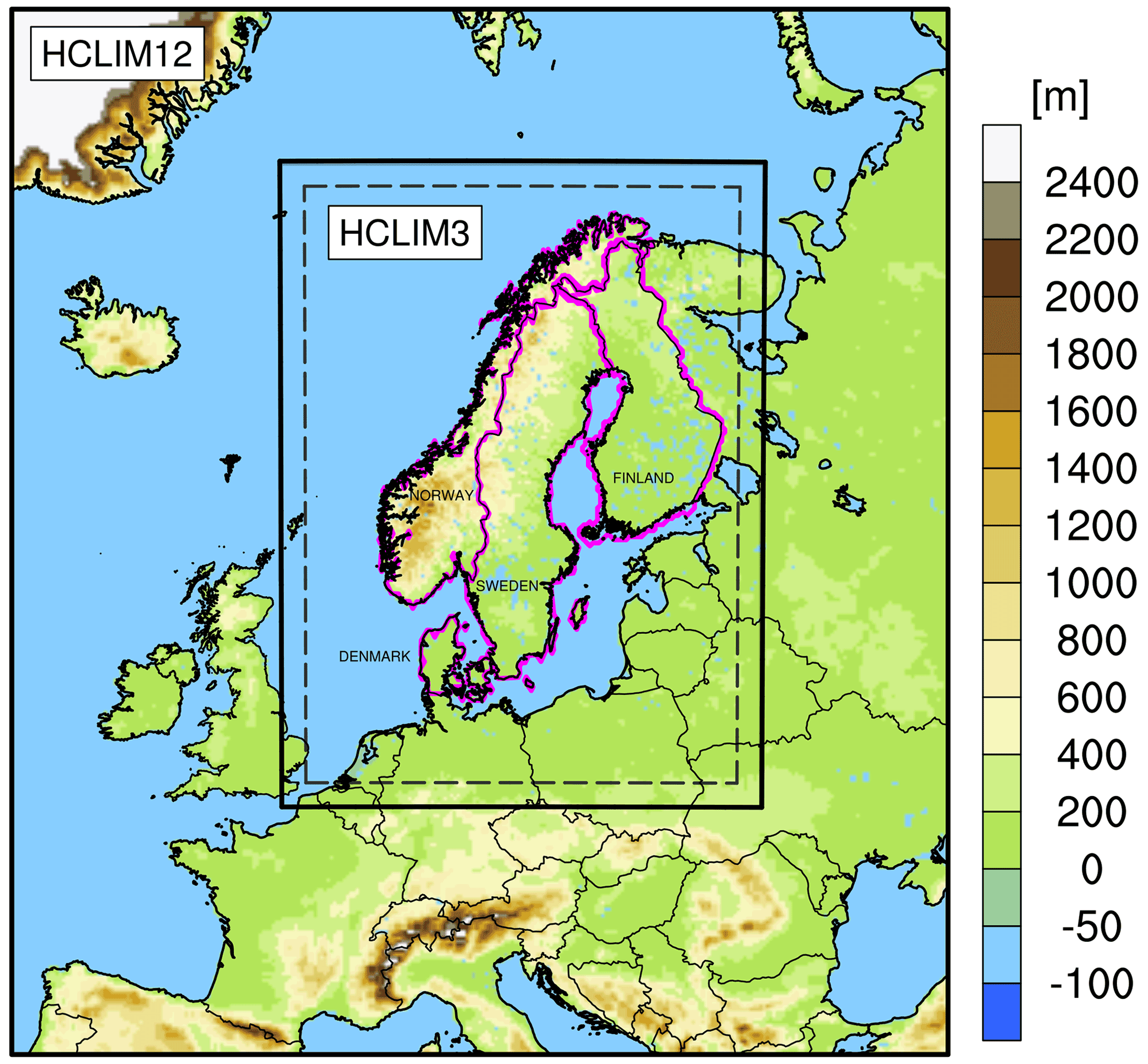
Figure 1The model domains of HCLIM12 (outer rectangle) and nested HCLIM3 (inner rectangle). The color scale represents the altitude in meters. The country borders used in the analysis are marked with magenta. The analyzed sub-domain is marked with a dashed outline.
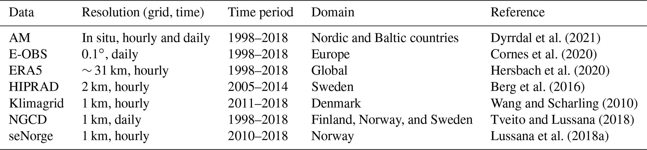
Table 1A summary of the observational datasets that were used in the model evaluation. The time period refers to the period used in this study. AM refers to the dataset of annual maximum precipitation.
2.1 Model and experiment setup
This study utilized the HCLIM38 regional climate model that is based on the ALADIN–HIRLAM (Aire Limitée Adaptation Dynamique Développement International–High Resolution Local Area Modelling) numerical weather prediction (NWP) system (Lindstedt et al., 2015; Bengtsson et al., 2017; Termonia et al., 2018). The model is presented only briefly here because it is thoroughly described in Belušić et al. (2020). The HCLIM38 modeling system contains different model configurations that are each suitable for different spatial scales. We employed two model setups, HCLIM38–AROME (Applications of Research to Operations at Mesoscale) at 3 km horizontal grid resolution and HCLIM38–ALADIN at 12 km horizontal grid resolution. HCLIM38–AROME is used with non-hydrostatic dynamics, as it is designed for convection-permitting resolutions (< 4 km) (Seity et al., 2011; Bengtsson et al., 2017). The recommended option in HCLIM38 for grid resolutions over 10 km is HCLIM38–ALADIN that is used with hydrostatic dynamics (Termonia et al., 2018). HCLIM38–ALADIN originates from the limited-area version of the global model ARPEGE (Action de Recherche Petite Échelle, Grande Échelle). From now on, HCLIM38–AROME at 3 km and HCLIM38–ALADIN at 12 km will be referred to as HCLIM3 and HCLIM12, respectively.
The experiment was performed using double nesting. The HCLIM12 run spans over a major part of Europe and the eastern North Atlantic with 313 × 349 horizontal grid points (Fig. 1), 65 vertical levels, and a time step of 300 s. The global ERA-Interim reanalysis with a grid resolution of ∼ 80 km (Dee et al., 2011) provided the boundary data for HCLIM12 every 6 h. HCLIM12 provided boundary data every 3 h for HCLIM3 that was run over the Nordic domain with 637 × 853 horizontal grid points, 65 vertical levels, and a time step of 75 s. The modeled periods covered 1997–2018, but the year 1997 was treated as a spin-up year and is thus not included in the analysis. Lind et al. (2020) provide more details of the experiments.
In the analysis, we focus mainly on the HCLIM3 domain. To account for the boundary effects, we removed approximately 100 km (33 grid points including the relaxation zone of 8 grid points) from each side of the HCLIM3 boundaries, which resulted in a domain that was analyzed in more detail (see the dashed outline in Fig. 1). Also, the HCLIM12 boundaries are adequately far away from the analyzed sub-domain (more than 500 km) (see, e.g., Denis et al., 2002; Matte et al., 2017).
2.2 Observations
The simulated daily precipitation was compared with gridded observational datasets, E-OBS and Nordic Gridded Climate Dataset (NGCD), as well as with high-resolution national gridded datasets (see Table 1 for references) that were also used to analyze the hourly precipitation. In addition, the hourly precipitation was compared with the ERA5 reanalysis dataset and in situ rain gauge data. We evaluated only land points, as most of the observational datasets are based on in situ gauge measurements over land. The used observational datasets and their references are summarized in Table 1 and described in more detail below.
The E-OBS dataset is based on the station series from the European Climate Assessment & Dataset (ECA&D) station network (Copernicus Climate Change Service, 2020). The dataset spans from 1950 until the present and covers a pan-European domain with a grid spacing of 0.1∘ × 0.1∘ (∼ 12 km). We utilized version 20.0e that consists of the ensemble means of 100-member realizations which can be taken as grid box averages (Cornes et al., 2020).
The NGCD dataset is a high-resolution dataset of gridded daily precipitation covering Finland, Sweden, and Norway (Tveito and Lussana, 2018; Copernicus Climate Change Service, 2021). The dataset covers a period from 1971 until the present and has a grid spacing of 1 km × 1 km. NGCD extends the national dataset of Norway, seNorge, that has been developed over the last 20 years (e.g., Tveito et al., 2005; Lussana et al., 2018a, b). The station data from Norway are extracted from the climate database of the Norwegian Meteorological Institute, while the Finnish and Swedish station data are extracted from ECA&D. We employed the NGCD version 19.03 and type 2 data that utilize the Bayesian interpolation method.
ERA5 is a reanalysis product based on a combination of data assimilation and numerical models (Hersbach et al., 2018, 2020). The dataset provides hourly precipitation at a horizontal grid spacing of approximately 30 km. Because the dataset was produced with a numerical model, it includes similar model deficiencies compared to other weather and climate models. The ERA5 forecast product has two separate initialization times, 06:00 UTC and 18:00 UTC. After initialization, the forecasts are run for 18 h. To account for and reduce the effects of model spin-up in precipitation, we utilized the 7–18 h forecast hours from the 06:00 UTC analysis (representing 13:00–00:00 UTC) and the 7–18 h forecast hours from the 18:00 UTC analysis (representing 01:00–12:00 UTC). A similar approach was used, e.g., in Crossett et al. (2020).
We utilized three national high-resolution gridded datasets, namely seNorge2 (seNorge hereafter), Klimagrid Danmark (Klimagrid hereafter), and HIPRAD v2 (High-Resolution Precipitation from Gauge-Adjusted Weather Radar; HIPRAD hereafter). The seNorge dataset provides hourly precipitation starting from 2010 with a grid spacing of 1 km over Norway (Lussana et al., 2018a; Norwegian Meteorological Institute, 2022). The dataset is based on in situ measurements that are interpolated using optimal interpolation and successive-correction schemes. Also, geographical coordinates and elevation are used as complementary information. The performance of this dataset is comparable to or even better than E-OBS, because of the higher effective resolution in seNorge (Lussana et al., 2018a). Despite this, seNorge underestimates precipitation over the mountainous region that has sparse data coverage. Klimagrid is a gauge-based gridded dataset with a grid spacing of 1 km over Denmark. The data consist of hourly precipitation for 2011–2019. At each time, an interpolation to the 1 km grid includes station information in all directions, weighted by distance; distance to the coastline is treated explicitly in the interpolation (Wang and Scharling, 2010). HIPRAD (Berg et al., 2016) is a gridded dataset covering Sweden with hourly resolution and a 2 km grid spacing. This dataset is based on radar data corrected by daily scaling factors using a 31 d running window and the PTHBV (Precipitation and Temperature for the Hydrologiska Byråns Vattenbalansavdelning hydrological model) gridded dataset for Sweden (Johansson and Chen, 2003). HIPRAD is available for 2000–2014, but due to gaps in the data, we utilized only the period of 2005–2014. In addition, grid points with suspected clutter effects were discarded from the analysis. These points were identified by comparing the distribution of daily intensity values of HIPRAD and its reference data, PTHBV, and matches based on the Perkins skill score (Perkins and Pitman, 2009) of the two probability density functions below 0.8 were rejected. In addition, we investigated the results from 102 in situ gauges over Sweden. However, the results were comparable to HIPRAD and are therefore not discussed in this paper.
We also utilized the daily and hourly annual maxima (AM) dataset that is extracted from in situ observations over the Nordic region (Dyrrdal, 2020). The daily data are available for Denmark, Finland, Norway, and Sweden for the years 1998–2018, while hourly maxima are available for Denmark, Norway, and Sweden covering the same period. Because this dataset includes only annual maxima, it could be used for the comparison of modeled return levels. The observations are extracted for each year utilizing all months, although the criteria for extraction varied between each country (Dyrrdal et al., 2021). For instance, the Swedish data were retrieved only if at maximum 2 d was missing from June to October, whereas the Norwegian data were extracted using a limit of 30 missing days per year. The Finnish and Danish data were extracted without any limits, but the plausibility of low values was checked. Annual maxima were extracted using all months also from the model and other observational datasets instead of limiting the analysis to April–September (see Sect. 3.1). The locations of the in situ stations can be found in Fig. S1a in the Supplement.
It is important to keep in mind that gridded and in situ observations of precipitation are prone to uncertainties. These uncertainties originate, for instance, from instrument errors, post-processing (interpolation methods, quality checks), and different spatial scales (e.g., comparison of point measurements with modeled areal averages) (Eggert et al., 2015) as well as a high spatiotemporal climatic variability of precipitation (e.g., Prein and Gobiet, 2017; Kotlarski et al., 2019). Furthermore, precipitation undercatch can be substantial for snowfall or windy conditions (e.g., Adam and Lettenmeier, 2003; Rubel and Hantel, 2001). Based on Rubel and Hantel (2001), the undercatch in the Baltic Sea area might be around 20 %–50 % during winter and 2 %–5 % during summer. Uncertainty is also introduced during the interpolation process of point measurements onto a regular grid. For instance, sparse data coverage and complex topography can lead to a large underestimation of precipitation (e.g., Prein and Gobiet, 2017). Moreover, interpolation can impose a smoothing effect on the spatial variability and lead to an underestimation of extremes (Hofstra et al., 2010). The national datasets, excluding Klimagrid, used in this study include mostly fewer stations compared to their corresponding daily records. They also cover shorter periods and include therefore more uncertainties compared to the daily products. It is also worth noting that most of the stations located in the Scandinavian mountains are established below 1000 m above sea level (m a.s.l.), although the terrain height can reach 2000 m a.s.l. or more (Lussana et al., 2019). This leads to uncertainties in precipitation values that are measured over mountainous areas and mountain ridges.
The NGCD dataset has been shown to underestimate precipitation exceeding 1, 10, and 25 mm d−1 by 5 %, 15 %, and 25 % on average, respectively, due to spatial smoothing (Tveito and Lussana, 2018). The correction factors for seNorge precipitation data have been estimated to vary between 0.7–3 depending on the region (Lussana et al., 2018a). The mean correction factor is 1.25, which means that precipitation is mainly underestimated by 25 %. The estimates of the effect of spatial smoothing were not available for Klimagrid, but precipitation from the gauge data in Denmark is underestimated by 1 %–2 % due to undercatch, which is lower for higher intensities (Vejen et al., 2021). There are no uncertainty estimates for HIPRAD v2, but the newest version of HIPRAD (v3) generally overestimates precipitation compared to gauge data (Olsson et al., 2021b). It needs to be noted that HIPRAD includes an undercatch correction that was not applied to the in situ stations. Because the uncertainty estimates vary between the datasets and different intensities, we do not consider one acceptable uncertainty range (see, e.g., Ban et al., 2021). Nevertheless, these uncertainties need to be kept in mind when analyzing the results.
To explore the effect of interpolation on the results, we additionally selected only the grid cells that included at least one weather station for further assessment. This so-called geographic sampling was performed for the seNorge and Klimagrid datasets. If a climate model has a horizontal resolution of tens of kilometers or below, there are likely grid cells where the model output is compared with an interpolated value instead of an actual measurement. This affects the evaluation of extreme precipitation as noted by Risser and Wehner (2020). However, Klimagrid is constructed to use exact station values in the grid points if there is not more than one station. In this case, the values for grid points containing one station are not areal averages but rather comparable to point measurements. Figure S1b in the Supplement shows the locations of the stations that were used for geographic sampling and that were available during the entire period in question, 2010–2018 for seNorge and 2011–2018 for Klimagrid.
We decided not to use so-called areal reduction factors (ARFs) for the in situ data. ARFs are generally used to take into account temporal and spatial differences in the observations and model. In our study, the area of one grid cell is 9 km2 in HCLIM3 and 144 km2 in HCLIM12. The adjustment needed for HCLIM3 can be considered small, whereas the adjustment could be over 10 % for HCLIM12 (Pavlovic et al., 2016). However, the literature proposes several different ways to adjust the values, which makes the use of adjustment factors uncertain. Therefore, we prefer not to adjust but rather assess the model outputs directly and comment in the text when needed.
3.1 Evaluation metrics of heavy precipitation
We analyzed daily and hourly heavy-precipitation events with intensity and time-based metrics. These metrics included the average of precipitation values above the 95th and 99.9th percentiles of all days or hours (hereafter pXavg) following Berthou et al. (2020) and frequencies of heavy-precipitation events of more than 10 mm d−1, 20 mm d−1, or 5 mm h−1 (hereafter R10mm, R20mm, and R5mm, respectively). R10mm and R20mm represent heavy- and very heavy-precipitation days, respectively, while R5mm represents heavy-precipitation hours. No threshold was used for the percentile computations as recommended by Schär et al. (2016). For the hourly scale, we also computed extra metrics that included the frequency distributions of precipitation intensity with a drizzle threshold of 0.1 mm h−1 as well as the diurnal cycle of the 99.9th percentile events. The percentiles were determined separately for each hour of the day. In this study, the term “heavy precipitation” is considered to represent the highest percentiles, whereas by “extreme precipitation” we mean either annual maximum precipitation or return levels obtained with extreme value analysis (see Sect. 3.2).
The seasonality of extreme-precipitation events was investigated by sampling the annual maxima of hourly and daily precipitation events for each year separately for a period from April to September and computing the monthly occurrences. A drizzle threshold of 0.1 mm h−1 was applied to the data, and similarly to Berg et al. (2019), a 24 h dry period was used between events so that the events can be considered independent.
All metrics were computed for a period from 1 April to 30 September over the overlapping years between the model and observations. The results were computed for each grid cell separately, and boxplots were used to show the spatial variability of the results. The results are shown mainly in the native grid. Remapping was performed prior to the analysis to the coarsest grid with a first-order conservative remapping method. However, remapped results did not change the conclusions and are therefore not discussed in more detail. If not stated otherwise, the differences between the HCLIM model (mod) and observations (obs) for a metric (M) were computed as relative biases (%):
3.2 Extreme value analysis
To gain insight into the extreme-precipitation events, we used extreme value analysis (Coles, 2001) at hourly and daily timescales. The analyzed period was 21 years (1998–2018), which was assumed to be stationary. We tested this assumption using the Kwiatkowski–Phillips–Schmidt–Shin (KPSS) test (Kwiatkowski et al., 1992). Based on this test, more than 90 % of the in situ stations and grid cells in the HCLIM model and gridded observations indicated stationary annual maximum values. The only exception was hourly Norwegian in situ data, of which 80 % were stationary.
The generalized extreme value (GEV) distribution was fitted to the annual maximum precipitation data to estimate return values. The cumulative distribution function of the GEV for a random variable (x) can be written as

Figure 2(a–d) Average daily precipitation above the 99.9th percentile (p99.9avg) in (a) E-OBS and the relative biases of p99.9avg values in (b) NGCD, (c) HCLIM12, and (d) HCLIM3 with a reference to E-OBS. (e–h) R20mm values in (e) E-OBS and the percentage points (model–observations) of R20mm values in (f) NGCD, (g) HCLIM12, and (h) HCLIM3 with a reference to E-OBS. The NGCD and HCLIM data were remapped onto E-OBS's grid prior to the analysis. Fldmean represents the average bias over the domain, and the values in brackets show the average bias over the NGCD domain. All units are in percentage except in (a), where the unit is millimeters per day.
This function is defined by three parameters (location μ, scale σ, and shape ξ) which were estimated with a modified maximum-likelihood method that utilizes a Bayesian prior distribution for the shape parameter (Martins and Stedinger, 2000; Frei et al., 2006). Several other studies have utilized this method (Frei et al., 2006; Rajczak et al., 2013; Rajczak and Schär, 2017; Ban et al., 2020) because it prevents the estimation of unrealistic shape parameters in case the sample size is small (Martins and Stedinger, 2000). Also, the L-moments method was tested for parameter estimation, but it yielded very similar results compared to the modified maximum likelihood. When the parameters are known, return values for different return periods can be estimated from the quantile function:
We computed return values for hourly (x1h) and daily (x1d) accumulated precipitation for return periods of T years (5, 10, and 20 years). We use abbreviations x1h.T and x1d.T to define the return values of 1 h and 1 d precipitation, respectively, for a return period of T. The goodness of fit was checked with the Kolmogorov–Smirnov (KS) test that compares the empirical distribution function with a specified distribution function, in this case, the GEV distribution. Based on the KS test, the GEV fit was adequately captured for more than 99.9 % of the grid cells or stations in the models and observations both at daily and hourly scales.
4.1 Evaluation of heavy daily precipitation
Both HCLIM12 and HCLIM3 underestimate p99.9avg by 10 %–30 % over areas where p99.9avg values are the highest in E-OBS (coastal Norway, south and north of Sweden, the central part of Finland, and Germany), while this metric is overestimated by 10 %–40 % over other parts of Finland, Sweden, and Norway (Fig. 2). Overall, the average relative bias over the domain is positive: 23 % for HCLIM12 and even greater in HCLIM3 with 44 %. The results are in line with previous studies in which HCLIM38 has been shown to overestimate mean daily precipitation at 12 km resolution by 25 %–28 % during the summer period over the Nordic region (Toivonen et al., 2019; Lind et al., 2020). In addition, Lind et al. (2020) showed that HCLIM3 improved the representation of the mean daily precipitation in the area. However, the differences compared to E-OBS in daily heavy precipitation seem to be larger in HCLIM3 than in HCLIM12 in the current study.
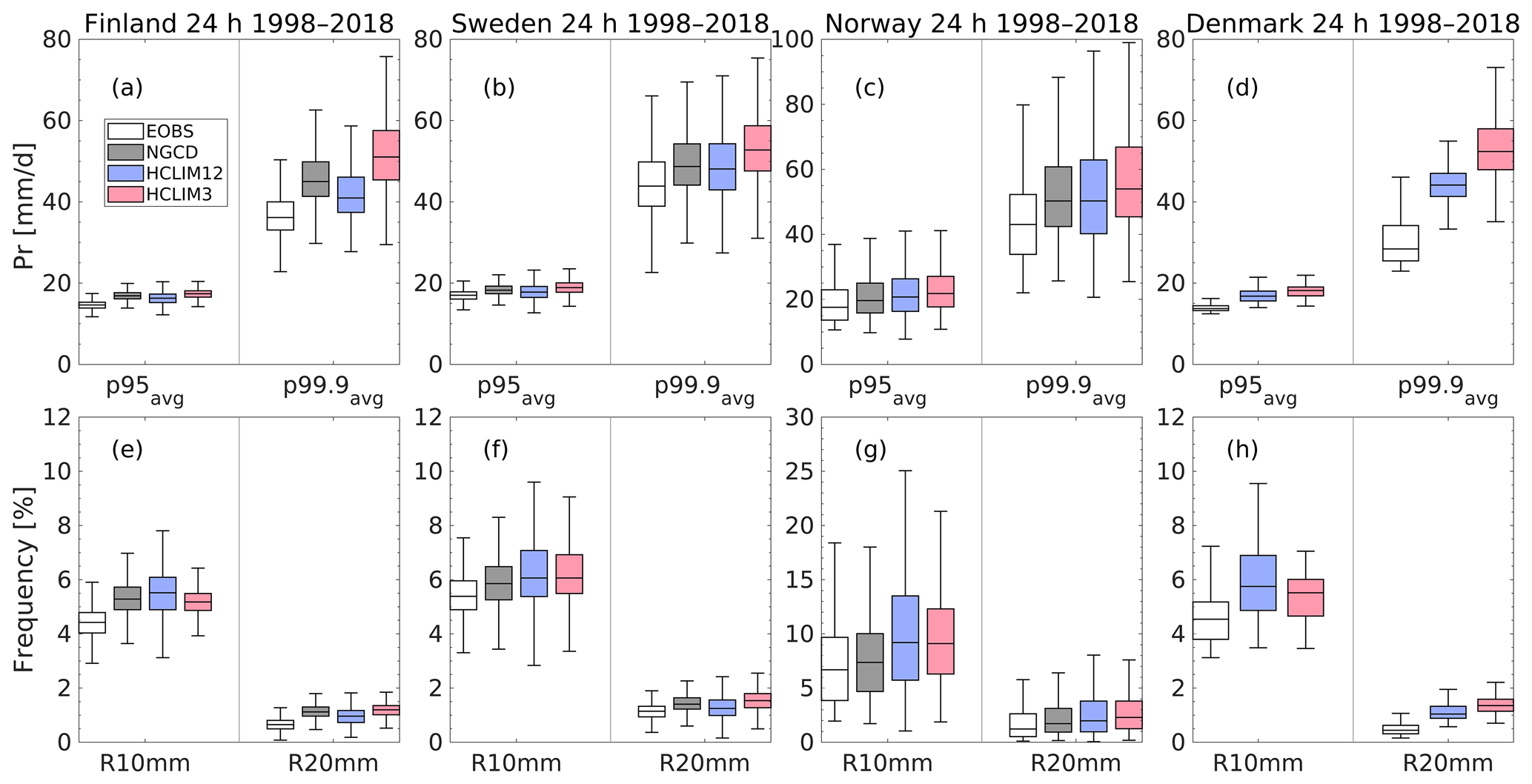
Figure 3(a–d) Average daily precipitation (Pr) over the 95th and 99.9th percentiles (p95avg and p99.9avg) in (a) Finland, (b) Sweden, (c) Norway, and (d) Denmark in HCLIM12, HCLIM3, and observational datasets. (e–h) The frequency of days with heavy (R10mm) and very heavy (R20mm) precipitation in HCLIM12, HCLIM3, and observational datasets in (e) Finland, (f) Sweden, (g) Norway, and (h) Denmark. The data are presented on their native grids. The central mark in the boxplots is the median, while the limits of the boxes represent the 25th percentile (Q1) and the 75th percentile (Q3), representing the interquartile range (IQR). The whiskers represent the range from Q1–1.5IQR to Q3+1.5IQR.
It is worthwhile to note that the high-resolution gridded observation set, NGCD, gives around 18 % higher p99.9avg values compared to E-OBS. Therefore, some part of the overestimation in HCLIM3 (25 % for p99.9avg over the NGCD domain) can be due to E-OBS failing to capture the most intense precipitation events. Furthermore, overestimation of more than 50 % in HCLIM12 and HCLIM3 can mostly be found in Denmark, the Baltic countries, and the eastern part of the analyzed domain. These areas have delivered less dense in situ station network data (see Fig. 1 in Cornes et al., 2020), which is argued to lead to smoothing of the extremes in the E-OBS dataset (Hofstra et al., 2010; Cornes et al., 2020). Previous studies have found similar issues when comparing mean precipitation from RCMs to E-OBS (Christensen et al., 2010).
The spatial distribution of the biases is similar for R20mm and p99.9avg (Fig. 2). It seems the average percentile values are underestimated over the same area where the very heavy-precipitation days are underestimated (the same applies to overestimation). The average bias of R20mm over the domain is positive for both HCLIM12 (0.4 %) and HCLIM3 (0.6 %). Again, NGCD has on average 0.3 % greater values compared to E-OBS. Negative biases of both p99.9avg and R20mm near the coastal regions might stem from model physics and, more specifically, micro-physics. Fixed values of cloud concentration nuclei (CCN) numbers are used in HCLIM: over the sea, over land, and over cities. Sensitivity results performed over Norway showed that the negative bias in mean-precipitation and extreme-precipitation events in the coastal regions could be improved by more realistic CCN values in the model, especially in cases when an air mass is moving from ocean to land (Landgren, 2020). However, more evaluation regarding the improvements in the extremes would be needed, as only two extreme-precipitation cases were studied.
Figure 3 presents the boxplots of the average daily precipitation values over the 95th and 99.9th percentiles (p95avg–p99.9avg, Fig. 3a–d) and the frequency of days with heavy (R10mm) and very heavy (R20mm) precipitation (Fig. 3e–h). Overall, the median values, as well as the variability of p95avg and p99.9avg, agree well between both HCLIM setups and the high-resolution NGCD dataset. Compared to the median values of p95avg–p99.9avg from NGCD (E-OBS in Denmark), HCLIM12 seemed to slightly underestimate the values in Finland and Sweden by 1 %–9 % and overestimate them in Norway and Denmark by 0 %–55 % (see Table S1 in the Supplement). The relative biases in HCLIM3 were mainly positive at 3 %–13 % (32 %–84 % in Denmark), with the largest biases being recorded for the greater percentile. The main features of the relative biases of p95avg–p99.9avg values, such as overestimation in HCLIM3 over all regions and underestimation in HCLIM12 over Finland and Sweden, were comparable with relative biases of the 70th to 99.99th percentiles of daily precipitation found in a study by Lind et al. (2020). In that study, HCLIM3 overestimated summertime (June–July–August) percentiles by 0 %–6 %, while HCLIM12 underestimated them by 6 %–13 % when compared to NGCD.
As shown in Fig. 3, HCLIM12 overestimates the variabilities of R10mm and R20mm values compared to NGCD (E-OBS in Denmark). HCLIM3, on the other hand, produces similar variabilities of R10mm and R20mm compared to observations, although it slightly underestimates the variabilities of R10mm in Finland and overestimates them in Sweden and Norway. Compared to the median values from the NGCD dataset (E-OBS in Denmark), HCLIM12 produces greater median values of R10mm leading to positive relative biases ranging from 3 % to 27 % (Table S1). HCLIM12 underestimates the very heavy-precipitation days (R20mm) in Finland and Sweden by 14 %–15 %, while these are overestimated over Norway and Denmark by 15 % and 135 %, respectively. HCLIM3 has mainly positive biases for both metrics: 4 %–24 % for R10mm (−2 % over Finland) and 7 %–206 % for R20mm.
The largest biases for p95avg–p99.9avg as well as for R10mm and R20mm values are seen for Denmark where the modeled values were compared to E-OBS instead of the high-resolution NGCD dataset. As discussed before, the ability of E-OBS to represent the heavy-precipitation events is questionable and might lead to misleading results. For instance, the relative biases in HCLIM3 and HCLIM12 decrease substantially from 22 %–206 % to ± 15 % when the modeled values over Denmark are compared with the national high-resolution dataset, Klimagrid, instead of E-OBS. Another aspect is the clear added value that can be found for HCLIM3 over Sweden when the modeled values are compared to the national high-resolution HIPRAD dataset instead of NGCD. When comparing the values to NGCD, it seems that the relative biases would be smaller in HCLIM12 than HCLIM3. However, a comparison with HIPRAD reveals that HCLIM12 greatly underestimates the observed values. At the same time, the assumed overestimation in HCLIM3 decreases. We note that the baseline used in constructing HIPRAD, namely PTHBV, includes a generic undercatch correction that might explain differences to NGCD. Also Hu et al. (2020) showed that E-OBS and ERA5 datasets underestimated the magnitude of daily extreme precipitation when compared to in situ data over Germany, while the national high-resolution dataset was able to represent the extremes adequately. On the other hand, E-OBS and NGCD cover larger regions and a longer time period compared to national high-resolution observations, which makes them worthwhile to consider in this study.
It is therefore worth noting that the model results should be compared with several different observations to get a more realistic overview of the model biases as already suggested by Prein and Gobiet (2017). They also emphasized the importance of local in situ measurements in evaluating the modeled statistics of extremes. However, also in situ measurements include uncertainties (e.g., related to undercatch). For instance, Crespi et al. (2019) noted that precipitation climatologies over Norway were improved by combining another HCLIM model output at 2.5 km grid spacing with in situ measurements instead of using only local observations. The climatologies were especially improved over remote mountainous regions. Similar conclusions were obtained in a study by Lundquist et al. (2019), who noted that precipitation from the model might be more accurate compared to observationally based datasets in complex terrain for mid to northern latitudes. Therefore, the overestimation in HCLIM3 could partly be caused by the inability of the gridded observations to represent the upper tails of precipitation distribution, especially over the Scandinavian mountains.
4.2 Evaluation of extreme daily precipitation
A noticeable feature seen in daily return values (Fig. 4) is the systematic difference between observational datasets. For all countries and return periods, the return values based on E-OBS are smaller than those from NGCD, which are in turn smaller than those from the collection of observational stations (i.e., the AM dataset; see Table 1). This is most pronounced for Denmark, where median return values from the AM dataset are larger than those from E-OBS by ∼ 50 %. The comparison between modeled and observed return values needs to be interpreted with this in mind.
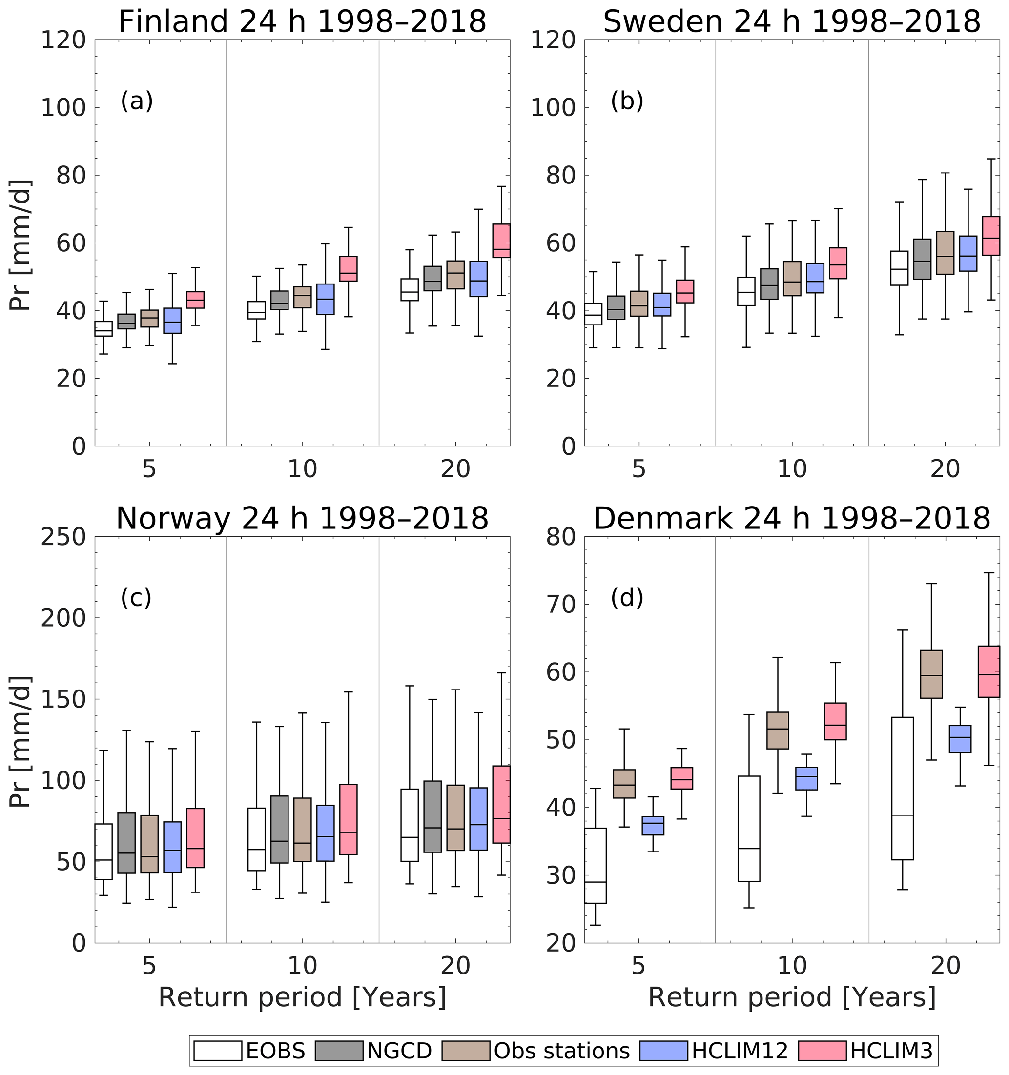
Figure 4Same as in Fig. 3 but for daily return levels in (a) Finland, (b) Sweden, (c) Norway, and (d) Denmark in HCLIM12, HCLIM3, and observational datasets. The label of Obs stations refers to the AM dataset.
HCLIM12 and HCLIM3 overestimate daily return values by 0 %–5 % and 5 %–21 %, respectively (> 30 % and 50 % in Denmark), compared to NGCD (E-OBS in Denmark) (Fig. 4, Table S1). The variability of return levels is mainly well captured by both HCLIM setups, although HCLIM12 overestimates the variability in Finland and underestimates it in Sweden and Norway. E-OBS seems to produce a spread of return values which is too large compared to in situ observations over Denmark. HCLIM3 produces variabilities similar to the Danish in situ data, whereas HCLIM12 underestimates them.
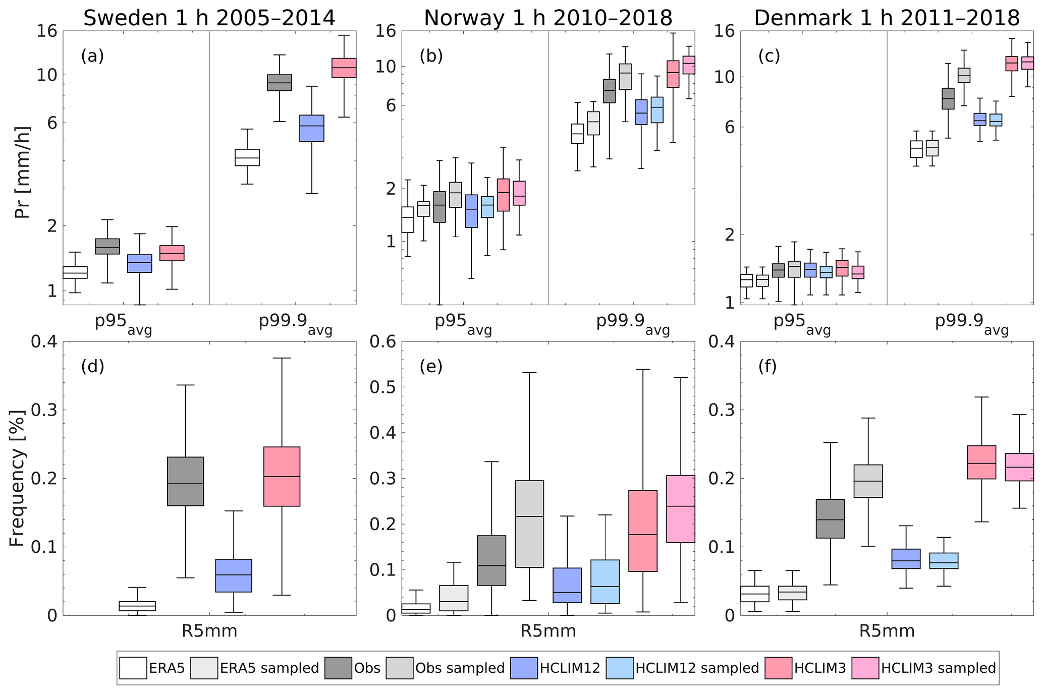
Figure 5(a–c) Same as in Fig. 3 but for average hourly precipitation over the 95th and 99.9th percentiles (p95avg and p99.9avg) in (a) Sweden, (b) Norway, and (c) Denmark in HCLIM12, HCLIM3, and observational high-resolution national datasets. Please note the logarithmic scale of the y axis. (d–f) The frequency of hours with heavy (R5mm) precipitation in HCLIM12, HCLIM3, and observational datasets in (d) Sweden, (e) Norway, and (f) Denmark. The label of Obs refers to the national high-resolution gridded datasets. The label of sampled refers to the results with geographic sampling.
The inadequacy of E-OBS observations in capturing the rarest extreme-precipitation events might explain the large differences in modeled return values when compared to E-OBS. This is confirmed when the model results are compared with the Danish in situ measurements: the relative biases are actually negative in HCLIM12 (around −15 %), meaning that this model setup does not capture very high intensities observed at the stations. Also, the relative biases in HCLIM3 decrease substantially. In Finland and Sweden, the results are similar between NGCD and in situ gauges, although the overestimation in HCLIM3 reduces slightly when the comparison is made against in situ stations instead of NGCD. Looking at the spatial distribution of the biases, negative biases in HCLIM12 can be found over Denmark and the coastal and mountainous areas of Norway and Sweden (Fig. S2 in the Supplement). Positive biases can be found in the inland areas in both model setups.
4.3 Evaluation of heavy hourly precipitation
The following sections show the evaluation of modeled hourly precipitation over Denmark, Norway, and Sweden for which the national high-resolution gridded observations were available. HCLIM3 mainly overestimates p95avg and p99.9avg by 3 %–44 % compared to national high-resolution observations (Fig. 5 and Table S2 in the Supplement), despite an underestimation of 6 % of p95avg in Sweden. On the contrary, HCLIM12 underestimates these metrics by 5 %–37 % and overestimates the p95avg by 1 % in Denmark. HCLIM3 also overestimates the precipitation events of more than 5 mm (R5mm) by around 60 % (5 % over Sweden), while HCLIM12 underestimates these events by 43 %–69 %. Also, Lind et al. (2020) and Olsson et al. (2021a) found mostly positive biases for hourly values over the 95th percentile in HCLIM3 and underestimation of the percentile values by HCLIM12.
HCLIM3 and HCLIM12 capture the variability of average values over all percentiles and R5mm, in spite of a slight overestimation over Sweden and Norway and underestimation over Denmark by HCLIM3. Furthermore, HCLIM12 overestimates the spread of p95avg and p99.9avg over Sweden, while the spread of R5mm is underestimated in all countries. The spatial distribution of the signs of the relative biases in p99.9avg and R5mm is very homogeneous: negative biases are found over all three countries in HCLIM12, whereas the biases are mainly positive in HCLIM3 throughout the domain despite some negative biases in the northern parts of Sweden and Norway (Fig. S3 in the Supplement). Furthermore, the spatial structure of the relative biases is very similar for p99.9avg and R5mm.

Figure 6The mean probability density functions of hourly precipitation for (a) Sweden, (b) Norway, and (c) Denmark. The shading presents the 25th and 75th percentiles from the spatial distribution. The label of Obs refers to the national high-resolution gridded datasets. All data are presented on their native grids. A threshold of 0.1 mm h−1 was used prior to analysis.
It should be noted that the ERA5 dataset did not capture the intensities or the spread of the average precipitation over the 95th and 99.9th percentiles well. Also, the R5mm values are substantially lower in ERA5 compared to the national high-resolution observations. This is not surprising, since ERA5 has a coarse grid resolution and parameterized convective precipitation. Therefore, ERA5 should be used with caution in the evaluation of extreme precipitation from convection-permitting climate models.
The comparison with geographically sampled observational grid cells (i.e., selecting only grid cells with stations) over Norway and Denmark reveals even more negative relative biases in HCLIM12 and decreasing relative biases in HCLIM3 of all metrics (p95avg–p99.9avg and R5mm; see Fig. 5 and Table S2). Without geographical sampling, the absolute relative biases of HCLIM12 seem to be lower than the biases of HCLIM3. When geographic sampling is accounted for, the biases are clearly lower in HCLIM3, while HCLIM12 considerably underestimates all metrics (Table S2). Geographical sampling could not be applied over Sweden, as the HIPRAD dataset is mainly based on radar observations. However, even when geographical sampling is performed, which is generally recommended by Risser and Wehner (2020), a scaling mismatch will still be present. This is because the scales of any station network will always be different from the scales of the horizontal resolutions and remaining sub-grid scale parameterizations in regional climate models.
Figure 6 presents probability density functions of hourly precipitation over Sweden, Norway, and Denmark. Added value can be found especially in the ability of HCLIM3 to represent the highest intensities in Sweden and Norway. HCLIM12, on the other hand, underestimates all intensities above 1.5–2 mm h−1 over all three countries compared to the national datasets. In Denmark, HCLIM3 shows overestimation for the highest intensities. With geographic sampling, the highest intensity (with a density of 0.001) computed from the observational Klimagrid data increases from 9 to 11 mm h−1, which is closer to the value simulated by HCLIM3 (∼ 12.5 mm h−1) than that of HCLIM12 (∼ 7.3 mm h−1) (Fig. S4b in the Supplement). Again, the added value found in HCLIM3 depends on the observational datasets that are used as a reference and can also be influenced by geographic sampling. The coarse-resolution ERA5 fails to capture the highest intensities compared to the higher-resolution observations.

Figure 7The mean diurnal cycles of the 99.9th percentile events for (a) Sweden, (b) Norway, and (c) Denmark. The shading presents the 25th and 75th percentiles from the spatial distribution. The label of Obs refers to the national high-resolution gridded datasets. The data are presented on their native grids.
The diurnal cycle of the 99.9th percentile is better represented in HCLIM3 compared to HCLIM12, especially over Sweden and Norway (Fig. 7). However, HCLIM3 shows some overestimation which is the largest during the daytime with a mean bias (model–observations) over all hours of 0.4 mm h−1 in Sweden, 0.8 mm h−1 in Norway, and 1.5 mm h−1 in Denmark (Table S2). HCLIM12 underestimates the precipitation intensities of all hours with a mean bias of −2.1 mm h−1 in Sweden, −0.9 mm h−1 in Norway, and −1.0 mm h−1 in Denmark. The observed peak in the 99.9th percentile precipitation occurs in the late afternoon in Sweden and Norway. There is no clear peak in observations in Denmark, but a minimum occurs during the night. Overall, the afternoon peak is well captured by HCLIM3 in Sweden and Norway, while the nighttime minimum in Denmark is not well represented. While HCLIM12 does not show any clear peaks, ERA5 shows peaks that are too early in Sweden and Norway. It is known that models with parameterized convection tend to produce peaks of the diurnal cycle that are ahead of time because the convection onset might be triggered too early (e.g., Brockhaus et al., 2008; Meredith et al., 2021). HCLIM12 and ERA5 also underestimate the observed intensities of the 99.9th percentile events throughout the day. Previously, Belušić et al. (2020), Lind et al. (2020), and Olsson et al. (2021a) have shown that HCLIM3 improved the representation of the diurnal cycles of mean precipitation as well as the 90th and 99th percentiles compared to HCLIM12.
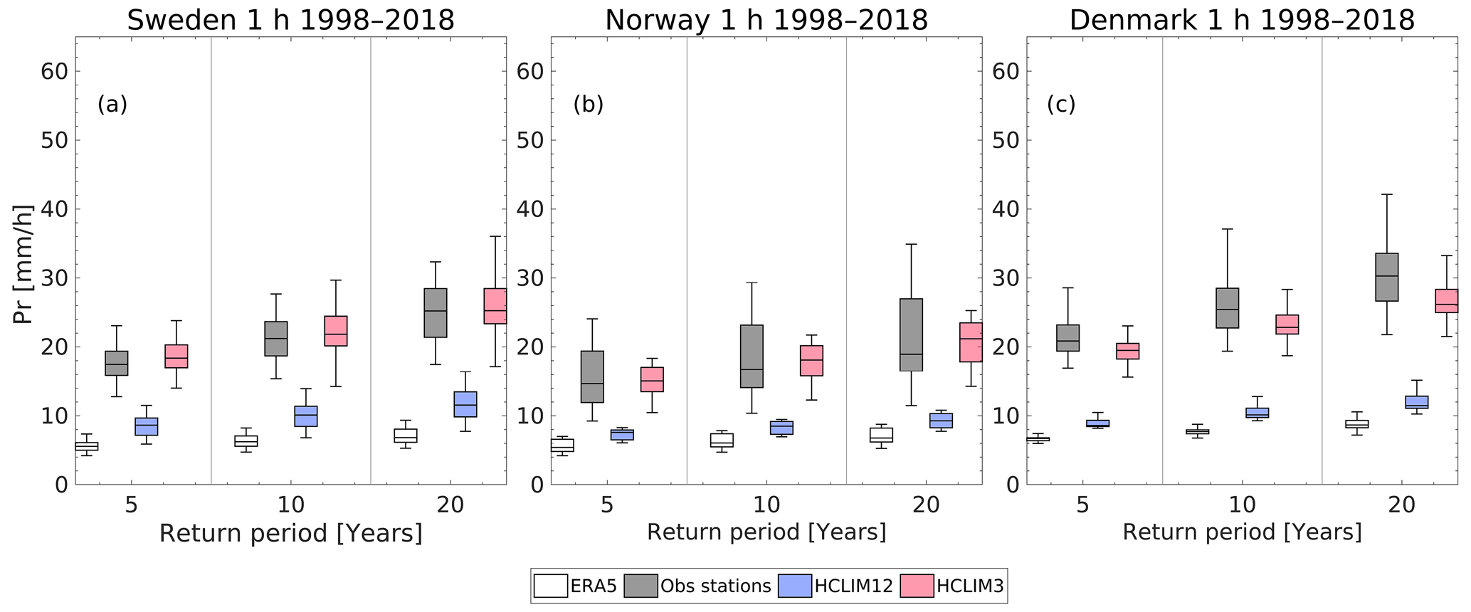
Figure 8Same as in Fig. 3 but for hourly return levels in (a) Sweden, (b) Norway, and (c) Denmark in HCLIM12, HCLIM3, and observational datasets. The label of Obs stations refers to the AM dataset.
When geographical sampling is applied, HCLIM3 better captures the shape of the diurnal cycle also over Denmark, although the nighttime minimum occurs still too late compared to observations (Fig. S4c and d). The mean bias in HCLIM3 decreases from 1.5 to 0.5 mm h−1 in Denmark and from 0.8 to 0.5 mm h−1 in Norway (Table S2). It is clear that involving all grid cells in the Klimagrid dataset deteriorates the comparison with HCLIM3. Lind et al. (2020) encountered similar problems in the ability of Klimagrid to capture the diurnal cycle of mean hourly precipitation. The problems might arise from the interpolation scheme used in Klimagrid, which interpolates spatially for each hour.
4.4 Evaluation of extreme hourly precipitation
HCLIM3 captures the hourly return levels of all return periods substantially better than HCLIM12 (Fig. 8). HCLIM12 underestimates all return levels by 48 %–62 %, while HCLIM3 has positive biases of 0 %–12 % in Sweden and Norway and negative biases of 7 %–14 % in Denmark (Table S2). Both model setups (especially HCLIM12) underestimate the variability of return periods over all countries, although HCLIM3 captures the variability over Sweden well. As expected, ERA5 shows poor performance in capturing the values and variabilities of all return levels compared to the in situ stations. The spatial structure of the relative biases of the return values with a return period of 10 years is very uniform in HCLIM12, as the biases are negative and of the same magnitude over all three countries (Fig. S5 in the Supplement). Positive and negative relative biases of HCLIM3 simulated return levels are irregularly scattered over the whole domain.
The underestimation of return levels and their variability by HCLIM3 and HCLIM12 might be too large because we did not take into account areal reduction factors for the in situ data. Statistical extremes retrieved from point sources (e.g., in situ gauges) are generally expected to be higher than extremes from climate models that produce spatial averages, which is causing a scaling mismatch (Chen and Knutson, 2008). Also, the differences in the temporal scales are not taken into account. The observed hourly precipitation is measured every 1 min in Denmark, every 15 min in Sweden, and every 1 min or 1 h in Norway, while the model produces values for every full hour. For instance, Berg et al. (2019) reported a reduction factor of 1.21 when going from a point measurement to a 12 km grid resolution and from 1 min temporal sampling time to 60 min. On the other hand, HCLIM3 would still show superior performance over HCLIM12 even if the hourly annual maxima from the in situ data would be reduced by 20 %.
The fact that most of the annual maximum precipitation occurs during the convective season in the summer (see Sect. 4.5; Lutz et al., 2020; Dyrrdal et al., 2021) indicates that the reason for the superior performance of HCLIM3 over HCLIM12 might be the explicitly resolved deep convection in HCLIM3. In addition, the results obtained for HCLIM12 are in line with previous studies. Berg et al. (2019) concluded that the regional climate model simulations with 12.5 km resolution underestimated 10-year return levels for hourly durations over selected European countries including Sweden.
Although Fig. 8 shows promising results from the convection-permitting regional climate model (CPRCM) setup, it would be important to assess the ability of the model to capture the actual meteorological conditions that lead to extreme-precipitation events. For instance, Coppola et al. (2020) showed that some specific observed extreme-precipitation cases might be missed by CPRCMs. Although CPRCMs generally cannot be expected to reproduce single extreme events even in perfect boundary simulations, they might simulate events that were “missed” by reality keeping in mind that reality is only one of the many realizations of climate. This leads to a better agreement of the long-term statistics of precipitation extremes between the model and observations. Olsson et al. (2021a) illustrated this point by analyzing how well the HCLIM model captured the observed extreme-precipitation event occurring in August 2014 in Malmö. They concluded that HCLIM3 reproduced the event but with reduced intensity. However, another event similar to the Malmö case was found in HCLIM3 but in a different year, whereas HCLIM12 did not simulate events of the same magnitude. It is good to note that a 21-year simulation period is a relatively short period, and one might need to wait more than 21 summers to generate the most intense precipitation events. Nonetheless, this calls for more studies of the underlying processes and meteorological conditions of the simulated extreme events, which would bring us forward regarding the shortcomings in models and observations.
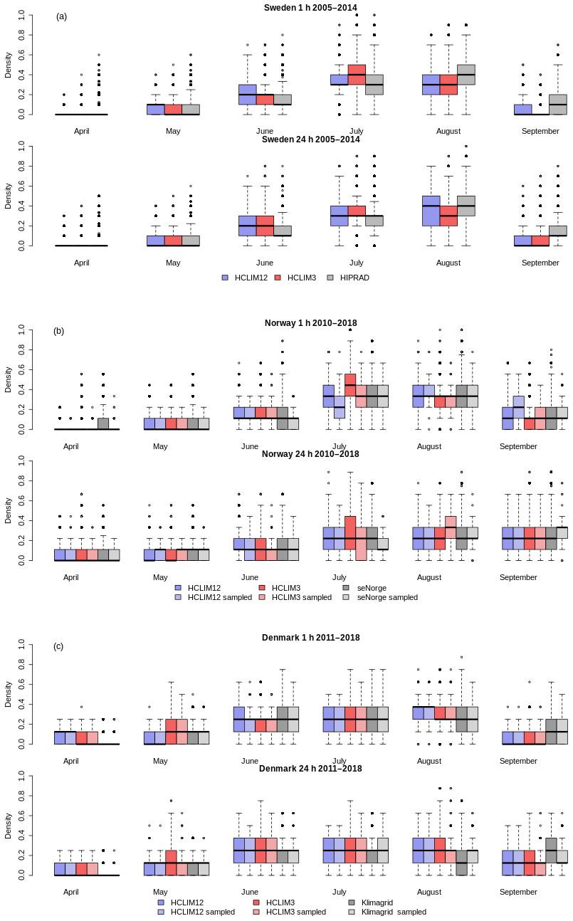
Figure 9Same as for Fig. 3 but for the distribution of monthly occurrences based on hourly and daily annual maximum precipitation in (a) Sweden, (b) Norway, and (c) Denmark in HCLIM12, HCLIM3, and observational datasets. The label of sampled refers to the results with geographic sampling.
4.5 Seasonality of hourly and daily annual maximum precipitation
Figure 9 illustrates the occurrences of simulated hourly and daily annual maximum precipitation in Sweden, Norway, and Denmark compared to the national high-resolution datasets. Annual hourly and daily extreme events are most frequent in July and August, except for daily events in Norway. In Norway, the daily extreme-precipitation events occur also in late autumn, especially near the coastal areas (Dyrrdal et al., 2021). Still, the larger density of occurrences in September in Norway is captured by both model setups. In addition, both HCLIM3 and HCLIM12 show good consistency with observational datasets, and overall, the differences resulting from the model setups are small.
HCLIM3 overestimates the occurrence of hourly extreme events in July over Sweden and Norway and, on the contrary, underestimates these events in August. Geographical sampling does not substantially affect the results, but for instance, the overestimated density of hourly events in July over Norway by HCLIM3 diminishes. Olsson et al. (2021a) encountered overestimated fractions of annual maxima observed in June and underestimated fractions in July and August by HCLIM3 and HCLIM12 over southern Sweden. However, they compared the results only over seven in situ stations in the specific area over Sweden, whereas this study considered the whole of Sweden. Although the results are not completely comparable, Olsson et al. (2021a) concluded that HCLIM3 did not improve the model performance regarding the monthly occurrences of annual maxima, which seems to be the case also in our study.
We analyzed the characteristics of heavy and extreme precipitation in 21-year-long convection-permitting climate simulations with non-hydrostatic dynamics at a 3 km grid spacing (HCLIM3) and compared them with climate simulations performed with 12 km grid spacing, hydrostatic dynamics, and parameterized convection (HCLIM12). These simulations have been evaluated and presented in previous studies (Lind et al., 2020; Olsson et al., 2021a), but this paper presents a more detailed evaluation of the extreme-precipitation statistics utilizing both basic metrics, such as average precipitation over the 95th to 99.9th percentiles and frequencies of heavy-precipitation events, as well as generalized extreme value (GEV) theory. The evaluation was performed over the Nordic region with a special focus on the warm season from April to September. The results are summarized as the following:
-
Daily heavy-precipitation amounts and frequencies, as well as daily return levels, were well represented over the Nordic region by HCLIM (at both 3 and 12 km grid spacings).
-
HCLIM3 was able to capture the most intense hourly precipitation events and their frequency with a slight overestimation, while these were underestimated by HCLIM12.
-
Overall, HCLIM3 improved the representation of the probability density functions of hourly precipitation and the diurnal cycle of the 99.9th percentile events over Sweden and Norway. In particular, the shape of the diurnal cycle, peak time, and amounts were better captured by HCLIM3, whereas the peak was not visible in HCLIM12.
-
A clear added value of HCLIM3 was seen in simulating return levels of hourly precipitation. HCLIM3 produced very similar precipitation intensities to in situ observations, while HCLIM12 substantially underestimated them.
-
Both models captured the seasonality of annual maximum precipitation with most of the daily and hourly events occurring in July and August.
This study confirmed that the coarser E-OBS and ERA5 datasets underestimate the most intense precipitation extremes in the Nordic region: the amounts and frequencies of heavy and extreme precipitation were substantially lower in these datasets compared to the high-resolution gridded observations. Therefore, the model results should be compared with several different datasets, preferably high-resolution ones or in situ observations, to get a better overview of the model biases. In general, part of the model biases might arise from the uncertainties in observations. The in situ network is sparse especially over Scandinavian mountains, and systematic undercatch of precipitation lowers the quality of observations in this region. Nevertheless, the results indicate that high-resolution observations are crucial in the evaluation of high-resolution climate models. The model evaluation would especially benefit from datasets that merge both rain gauges and high-resolution temporally and spatially continuous weather radar data as well as from better uncertainty estimates for the observational datasets. Also, geographic sampling affected the results of model evaluation: the sampling decreased the overestimation in HCLIM3 and led to a greater underestimation of the observed values by HCLIM12. The hourly heavy-precipitation intensities and amounts as well as the shape of the diurnal cycle were clearly better represented in HCLIM3 compared to HCLIM12 when geographic sampling was applied.
The results presented in this study generally agree with previous studies of evaluation of convection-permitting regional climate models. These include a better representation of the diurnal cycle and the highest intensities of hourly precipitation and their frequencies in convection-permitting HCLIM3. Hence, we conclude that an added value can be found for the HCLIM38 model at convection-permitting scales in simulating heavy- and extreme-precipitation events over the Nordic region. Although investigating the origin of the added value in HCLIM3 is beyond the scope of this study, the results indicate that the improvements in HCLIM3 are due to explicitly simulated deep convection. The higher horizontal resolution might also play a role. However, understanding the underlying processes of precipitation extremes would be highly beneficial to gain information on the ability of the model to reproduce these events for the right reasons. Nonetheless, the results indicate that high-resolution convection-permitting climate models are valuable for the construction of the future projections of extreme precipitation, as climate adaptation requires more robust and reliable projections of future changes. Future work will investigate the changing characteristics of precipitation extremes due to climate change over northern Europe with HCLIM3 and HCLIM12 while putting the results in context by comparing the HCLIM38 model with a larger RCM ensemble.
The ALADIN and HIRLAM consortia cooperate on the development of a shared system of model codes. The HCLIM model configuration forms part of this shared ALADIN–HIRLAM system. According to the ALADIN–HIRLAM collaboration agreement, all members of the ALADIN and HIRLAM consortia are allowed to license the shared ALADIN–HIRLAM codes within their home country for non-commercial research. Access to the HCLIM codes can be obtained by contacting one of the member institutes of the HIRLAM consortium (see links at http://hirlam.org/index.php/hirlam-programme-53, Lantsheer, 2016). The access will be subject to signing a standardized ALADIN–HIRLAM license agreement (http://hirlam.org/index.php/hirlam-programme-53/access-to-the-models, HIRLAM, 2022). Some parts of the ALADIN–HIRLAM codes can be obtained by non-members through specific licenses, such as in OpenIFS (Integrated Forecasting System; https://confluence.ecmwf.int/display/OIFS, Carver, 2022) and Open-SURFEX (Surface Externalisée; https://www.umr-cnrm.fr/surfex, SURFEX, 2022).
The E-OBS dataset is available at https://doi.org/10.24381/cds.151d3ec6 (Copernicus Climate Change Service, 2020). The ERA5 reanalysis dataset is available at https://doi.org/10.24381/cds.adbb2d47 (Hersbach et al., 2018). The NGCD dataset is available at https://doi.org/10.24381/cds.e8f4a10c (Copernicus Climate Change Service, 2021). The seNorge dataset is available at https://thredds.met.no/thredds/catalog/senorge/seNorge2/catalog.html (Norwegian Meteorological Institute, 2022). The dataset of annual maximum daily precipitation is available at https://doi.org/10.11582/2020.00023 (Dyrrdal, 2020). All other data and material are available upon request.
The supplement related to this article is available online at: https://doi.org/10.5194/nhess-22-693-2022-supplement.
EM designed and wrote the manuscript with contributions from ET and all co-authors. The analysis was performed by EM with the help of PL, and ET performed the seasonality analysis. All co-authors participated in the editing of the paper.
The contact author has declared that neither they nor their co-authors have any competing interests.
Publisher's note: Copernicus Publications remains neutral with regard to jurisdictional claims in published maps and institutional affiliations.
The HCLIM simulations were performed by the NorCP (Nordic Convection Permitting Climate Projections) project group, a collaboration between the Danish Meteorological Institute (DMI), Finnish Meteorological Institute (FMI), Norwegian Meteorological Institute (MET Norway), and the Swedish Meteorological and Hydrological Institute (SMHI). We acknowledge the storage resource Bi provided by the Swedish National Infrastructure for Computing (SNIC) at the Swedish National Supercomputing Centre (NSC) at Linköping University. We acknowledge the providers of the observational datasets used in this study. We are also thankful to Anita V. Dyrrdal, Antti Mäkelä, and Fuxing Wang for commenting on the first version of the manuscript.
This research has been supported by the Academy of Finland (grant nos. 329241, 337552, and 342561), the Maj ja Tor Nesslingin Säätiö (Maj and Tor Nessling Foundation), Horizon 2020 (with partial funding for the Swedish Meteorological and Hydrological Institute – SMHI – and the Danish Meteorological Institute – DMI – for European Climate Prediction – EUCP; grant no. 776613), the National Centre for Climate Research (NCKF), and the Svenska Forskningsrådet Formas (Swedish Research Council for Sustainable Development; grant no. 2018-02434).
This paper was edited by Joaquim G. Pinto and reviewed by two anonymous referees.
Adam, J. C. and Lettenmeier, D. P.: Adjustment of global gridded precipitation for systematic bias, J. Geophys. Res., 108, 4257, https://doi.org/10.1029/2002JD002499, 2003.
Ban, N., Schmidli, J., and Schär, C.: Heavy precipitation in a changing climate: Does short-term summer precipitation increase faster?, Geophys. Res. Lett., 42, 1165–1172, https://doi.org/10.1002/2014GL062588, 2015.
Ban, N., Rajczak, J., Schmidli, J., and Schär, C.: Analysis of Alpine precipitation extremes using generalized extreme value theory in convection-resolving climate simulations, Clim. Dynam., 55, 61–75, https://doi.org/10.1007/s00382-018-4339-4, 2020.
Ban, N., Caillaud, C., Coppola, E., Pichelli, E., Sobolowski, S., Adinolfi, M., Ahrens, B., Alias, A., Anders, I., Bastin, S., Belušić, D., Berthou, S., Brisson, E., Cardoso, R. M., Chan, S. C., Christensen, O. B., Fernández, J., Fita, L., Frisius, T., Gašparac, G., Giorgi, F., Goergen, K., Haugen, J. E., Hodnebrog, Ø., Kartsios, S., Katragkou, E., Kendon, E. J., Keuler, K., Lavin-Gullon, A., Lenderink, G., Leutwyler, D., Lorenz, T., Maraun, D., Mercogliano, P., Milovac, J., Panitz, H.-J., Raffa, M., Remedio, A. R., Schär, C., Soares, P. M. M., Srnec, L., Steensen, B. M., Stocchi, P., Tölle, M. H., Truhetz, H., Vergara-Temprado, J., de Vries, H., Warrach-Sagi, K., Wulfmeyer, V., and Zander, M. J.: The first multi-model ensemble of regional climate simulations at kilometer-scale resolution, part I: evaluation of precipitation, Clim. Dynam., 57, 275–302, https://doi.org/10.1007/s00382-021-05708-w, 2021.
Belušić, D., de Vries, H., Dobler, A., Landgren, O., Lind, P., Lindstedt, D., Pedersen, R. A., Sánchez-Perrino, J. C., Toivonen, E., van Ulft, B., Wang, F., Andrae, U., Batrak, Y., Kjellström, E., Lenderink, G., Nikulin, G., Pietikäinen, J.-P., Rodríguez-Camino, E., Samuelsson, P., van Meijgaard, E., and Wu, M.: HCLIM38: a flexible regional climate model applicable for different climate zones from coarse to convection-permitting scales, Geosci. Model Dev., 13, 1311–1333, https://doi.org/10.5194/gmd-13-1311-2020, 2020.
Bengtsson, L., Andrae, U., Aspelien, T., Batrak, Y., Calvo, J., de Rooy, W., Gleeson, E., Hansen-Sass, B., Homleid, M., Hortal, M., Ivarsson, K.-I., Lenderink, G., Niemelä, S., Nielsen, K. P., Onvlee, J., Rontu, L., Samuelsson, P., Muñoz, D. S., Subias, A., Tijm, S., Toll, V., Yang, X., and Køltzow, M. Ø.: The HARMONIE–AROME Model Configuration in the ALADIN–HIRLAM NWP System, Mon. Weather Rev., 145, 1919–1935, https://doi.org/10.1175/MWR-D-16-0417.1, 2017.
Beranová, R., Kyselý, J., and Hanel, M.: Characteristics of sub-daily precipitation extremes in observed data and regional climate model simulations, Theor. Appl. Climatol., 132, 515–527, https://doi.org/10.1007/s00704-017-2102-0, 2018.
Berg, P., Norin, L., and Olsson, J.: Creation of a high resolution precipitation data set by merging gridded gauge data and radar observations for Sweden, J. Hydrol., 541, 6–13, https://doi.org/10.1016/j.jhydrol.2015.11.031, 2016.
Berg, P., Christensen, O. B., Klehmet, K., Lenderink, G., Olsson, J., Teichmann, C., and Yang, W.: Summertime precipitation extremes in a EURO-CORDEX 0.11∘ ensemble at an hourly resolution, Nat. Hazards Earth Syst. Sci., 19, 957–971, https://doi.org/10.5194/nhess-19-957-2019, 2019.
Berthou, S., Kendon, E., Chan, S., Ban, N., Leutwyler, D., Schär, C., and Fosser, G.: Pan-European climate at convection-permitting scale: a model intercomparison study, Clim. Dynam., 55, 35–59, https://doi.org/10.1007/s00382-018-4114-6, 2020.
Boberg, F., Berg, P., Thejll, P., Gutowski, W. J., and Christensen, J. H.: Improved confidence in climate change projections of precipitation further evaluated using daily statistics from ENSEMBLES models, Clim. Dynam., 35, 1509–1520, https://doi.org/10.1007/s00382-009-0683-8, 2010.
Brockhaus, P., Lüthi, D., and Schär, C.: Aspects of the diurnal cycle in a regional climate model, Meteorol. Z., 17, 433–443, https://doi.org/10.1127/0941-2948/2008/0316, 2008.
Carver, G.: OpenIFS Home, 2020, https://confluence.ecmwf.int/display/OIFS, last access: 23 February 2022.
Caillaud, C., Somot, S., Alias, A., Bernard-Bouissières, I., Fumière, Q., Seity, Y., and Ducrocq, V.: Modelling Mediterranean heavy precipitation events at climate scale: an object-oriented evaluation of the CNRM-AROME convection-permitting regional climate model, Clim. Dynam., 56, 1717–1752, https://doi.org/10.1007/s00382-020-05558-y, 2021.
Chen, C.-T. and Knutson, T.: On the verification and comparison of extreme rainfall indices from climate models, J. Climate, 21, 1605–1621, https://doi.org/10.1175/2007JCLI1494.1, 2008.
Christensen, J. and Christensen, O.: Severe summertime flooding in Europe, Nature, 421, 805–806, https://doi.org/10.1038/421805a, 2003.
Christensen, J. H., Kjellström, E., Giorgi, F., Lenderink, G., and Rummukainen, M.: Weight assignment in Regional Climate Models, Clim. Res., 44, 179–194, https://doi.org/10.3354/cr00916, 2010.
Coles, S.: An Introduction to Statistical Modeling of Extreme Values, Springer-Verlag, London, Berlin, Heidelberg, 209 pp., 2001.
Copernicus Climate Change Service (C3S): E-OBS daily gridded meteorological data for Europe from 1950 to present derived from in-situ observations, Copernicus Climate Change Service (C3S) Climate Data Store (CDS) [data set], https://doi.org/10.24381/cds.151d3ec6, 2020.
Copernicus Climate Change Service (C3S): Nordic gridded temperature and precipitation data from 1971 to present derived from in-situ observations, Copernicus Climate Change Service (C3S) Climate Data Store (CDS) [data set], https://doi.org/10.24381/cds.e8f4a10c, 2021.
Coppola, E., Sobolowski, S., Pichelli, E., Raffaele, F., Ahrens, B., Anders, I., Ban, N., Bastin, S., Belda, M., Belusic, D., Caldas-Alvarez, A., Cardoso, R., Davolio, S., Dobler, A., Fernandez, J., Fita, L., Fumiere, Q., Giorgi, F., Goergen, K., Güttler, I., Halenka, T., Heinzeller, D., Hodnebrog, Ø., Jacob, D., Kartsios, S., Katragkou, E., Kendon, E., Khodayar, S., Kunstmann, H., Knist, S., Lavín-Gullón, A., Lind, P., Lorenz, T., Maraun, D., Marelle, L., van Meijgaard, E., Milovac, J., Myhre, G., Panitz, H., Piazza, M., Raffa, M., Raub, T., Rockel, B., Schär, C., Sieck, K., Soares, P., Somot, S., Srnec, L., Stocchi, P., Tölle, M., Truhetz, H., Vautard, R., de Vries, H., and Warrach-Sagi, K.: A first-of-its-kind multi-model convection permitting ensemble for investigating convective phenomena over Europe and the Mediterranean, Clim. Dynam., 55, 3–34, https://doi.org/10.1007/s00382-018-4521-8, 2020.
Cornes, R., van der Schrier, G., van den Besselaar, E. J. M., and Jones, P. D.: An Ensemble Version of the E-OBS Temperature and Precipitation Datasets, J. Geophys. Res.-Atmos., 123, 9381–9409, https://doi.org/10.1029/2017JD028200, 2020.
Crespi, A., Lussana, C., Brunetti, M., Dobler, A., Maugeri, M., and Tveito, O. E.: High-resolution monthly precipitation climatologies over Norway (1981–2010): joining numerical model data sets and in situ observations, Int. J. Climatol., 39, 2057–2070, https://doi.org/10.1002/joc.5933, 2019.
Crossett, C. C., Betts, A. K., Dupigny-Giroux, L.-A. L., and Bomblies, A.: Evaluation of Daily Precipitation from the ERA5 Global Reanalysis against GHCN Observations in the Northeastern United States, Climate, 8, 148, https://doi.org/10.3390/cli8120148, 2020.
Dee, D. P., Uppala, S. M., Simmons, A. J., Berrisford, P., Poli, P., Kobayashi, S., Andrae, U., Balmaseda, M. A., Balsamo, G., Bauer, P., Bechtold, P., Beljaars, A. C., van de Berg, L., Bidlot, J., Bormann, N., Delsol, C., Dragani, R., Fuentes, M., Geer, A. J., Haimberger, L., Healy, S. B., Hersbach, H., Hólm, E. V., Isaksen, L., Kållberg, P., Köhler, M., Matricardi, M., McNally, A. P., Monge-Sanz, B. M., Morcrette, J., Park, B., Peubey, C., de Rosnay, P., Tavolato, C., Thépaut, J., and Vitart, F.: The ERA-Interim reanalysis: configuration and performance of the data assimilation system, Q. J. Roy. Meteor. Soc., 137, 553–597, https://doi.org/10.1002/qj.828, 2011.
Denis, B., Laprise, R., Caya, D., and Côté, J.: Downscaling ability of one-way nested regional climate models: the Big-Brother Experiment, Clim. Dynam., 18, 627–646, https://doi.org/10.1007/s00382-001-0201-0, 2002.
Dyrrdal, A.: Annual maximum daily precipitation for the Nordic-Baltic countries, NIRD [data set], https://doi.org/10.11582/2020.00023, 2020.
Du, H., Alexander, L., Donat, M., Lippmann, T., Srivastava, A., Salinger, J., Kruger, A., Choi, G., He, H. S., Fujibe, F., Rusticucci, M., Nandintsetseg, B., Manzanas, R., Rehman, S., Abbas, F., Zhai, P., Yabi, I., Stambaugh, M. C., Wang, S., Batbold, A., de Oliveira, P. T., Adrees, M., Hou, W., Zong, S., Santos e Silva, C. M. S., Lucio, P. S., and Wu, F.: Precipitation From Persistent Extremes is Increasing in Most Regions and Globally, Geophys. Res. Lett., 46, 6041–6049, https://doi.org/10.1029/2019gl081898, 2019.
Dyrrdal, A., Olsson, J., Médus, E., Arnbjerg-Nielsen, K., Post, P., Aņiskeviča, S., Førland, E. J., Thorndahl, S., Lennart, W., Mačiulytė, V., and Mäkelä, A.: Observed changes in heavy daily precipitation over the Nordic-Baltic region, J. Hydrol. Reg. Stud., 38, 100965, https://doi.org/10.1016/j.ejrh.2021.100965, 2021.
Eggert, B., Berg, P., Haerter, J. O., Jacob, D., and Moseley, C.: Temporal and spatial scaling impacts on extreme precipitation, Atmos. Chem. Phys., 15, 5957–5971, https://doi.org/10.5194/acp-15-5957-2015, 2015.
Fosser, G., Khodayar, S., and Berg, P.: Benefit of convection permitting climate model simulations in the representation of convective precipitation, Clim. Dynam., 44, 45–60, https://doi.org/10.1007/s00382-014-2242-1, 2015.
Fowler, H. J., Lenderink, G., Prein, A. F., Westra, S., Allan, R. P., Ban, N., Barbero, R., Berg, P., Blenkinsop, S., Do, H. X., Guerreiro, S., Haerter, J. O., Kendon, E. J., Lewis, E., Schär, C., Sharma, A., Villarini, G., Wasko, C., and Zhang, X.: Anthropogenic intensification of short-duration rainfall extremes, Nat. Rev. Earth Environ., 2, 107–122, https://doi.org/10.1038/s43017-020-00128-6, 2021.
Førland, E. J., Alexandersson, H., Drebs, A., Hanssen-Bauer, I., Vedin, H., and Tveito, O. E.: Trends in maximum 1-day precipitation in the Nordic region, MET Norway report 14/98, 53 pp., Norwegian Meteorological Institute, Oslo, Norway, 1998.
Frei, C., Schöll, R., Fukutome, S., Schmidli, J., and Vidale, P.: Future change of precipitation extremes in Europe: Intercomparison of scenarios from regional climate models, J. Geophys. Res.-Atmos., 111, D06105, https://doi.org/10.1029/2005JD005965, 2006.
Fumière, Q., Déqué, M., Nuissier, O., Somot, S., Alias, A., Caillaud, C., Laurantin, O., and Seity, Y.: Extreme rainfall in Mediterranean France during the fall: added value of the CNRM-AROME Convection-Permitting Regional Climate Model, Clim. Dynam., 55, 77–91, https://doi.org/10.1007/s00382-019-04898-8, 2020.
Gregersen, I., Sørup, H., Madsen, H., Rosbjerg, D., Mikkelsen, P., and Arnbjerg-Nielsen, K.: Assessing future climatic changes of rainfall extremes at small spatio-temporal scales, Climatic Change, 118, 783–797, https://doi.org/10.1007/s10584-012-0669-0, 2013.
Hanel, M. and Buishand, T.: On the value of hourly precipitation extremes in regional climate model simulations, J. Hydrol., 393, 265–273, https://doi.org/10.1016/j.jhydrol.2010.08.024, 2010.
Hersbach, H., Bell, B., Berrisford, P., Biavati, G., Horányi, A., Muñoz Sabater, J., Nicolas, J., Peubey, C., Radu, R., Rozum, I., Schepers, D., Simmons, A., Soci, C., Dee, D., and Thépaut, J.-N.: ERA5 hourly data on single levels from 1979 to present, Copernicus Climate Change Service (C3S) Climate Data Store (CDS) [data set], https://doi.org/10.24381/cds.adbb2d47, 2018 (updated 2022).
Hersbach, H., Bell, B., Berrisford, P., Hirahara, S., Horányi, A., Muñoz-Sabater, J., Nicolas, J., Peubey, C., Radu, R., Schepers, D., Simmons, A., Soci, C., Abdalla, S., Abellan, X., Balsamo, G., Bechtold, P., Biavati, G., Bidlot, J., Bonavita, M., Chiara, G., Dahlgren, P., Dee, D., Diamantakis, M., Dragani, R., Flemming, J., Forbes, R., Fuentes, M., Geer, A., Haimberger, L., Healy, S., Hogan, R. J., Hólm, E., Janisková, M., Keeley, S., Laloyaux, P., Lopez, P., Lupu, C., Radnoti, G., Rosnay, P., Rozum, I., Vamborg, F., Villaume, S., and Thépaut, J. N.: The ERA5 global reanalysis, Q. J. Roy. Meteor. Soc., 146, 1999–2049, https://doi.org/10.1002/qj.3803, 2020.
HIRLAM: Access to the models, http://hirlam.org/index.php/hirlam-programme-53/access-to-the-models, last access: 23 February 2022.
Hofstra, N., New, M., and McSweeney, C.: The influence of interpolation and station network density on the distributions and trends of climate variables in gridded daily data, Clim. Dynam., 35, 841–858, https://doi.org/10.1007/s00382-009-0698-1, 2010.
Hu, G. and Franzke, C. L. E.: Evaluation of daily precipitation extremes in reanalysis and gridded observation-based data sets over Germany, Geophys. Res. Lett., 47, e2020GL089624, https://doi.org/10.1029/2020GL089624, 2020.
Johansson, B. and Chen, D.: The influence of wind and topography on precipitation distribution in Sweden: statistical analysis and modelling, Int. J. Climatol., 23, 1523–1535, https://doi.org/10.1002/joc.951, 2003.
Kendon, E., Roberts, N., Fowler, H., Roberts, M., Chan, S., and Senior, C.: Heavier summer downpours with climate change revealed by weather forecast resolution model, Nat. Clim. Change, 4, 570–576, https://doi.org/10.1038/nclimate2258, 2014.
Kendon, E., Ban, N., Roberts, N., Fowler, H., Roberts, M., Chan, S., Evans, J., Fosser, G., and Wilkinson, J.: Do Convection-Permitting Regional Climate Models Improve Projections of Future Precipitation Change?, B. Am. Meteorol. Soc., 98, 79–93, https://doi.org/10.1175/BAMS-D-15-0004.1, 2017.
Kotlarski, S., Szabó, P., Herrera, S., Räty, O., Keuler, K., Soares, P. M., Cardoso, R. M., Bosshard, T., Pagé, C., Boberg, F., Gutiérrez, J. M., Isotta, F. A., Jaczewski, A., Kreienkamp, F., Liniger, M. A., Lussana, C., and Pianko-Kluczyńska, K.: Observational uncertainty and Regional Climate Model Evaluation: A pan-European Perspective, Int. J. Climatol., 39, 3730–3749, https://doi.org/10.1002/joc.5249, 2019.
Kwiatkowski, D., Phillips, P. C. B., Schmidt, P., and Shin, Y.: Testing the null hypothesis of stationarity against the alternative of a unit root: How sure are we that economic time series have a unit root?, J. Econometrics, 54, 159–178, https://doi.org/10.1016/0304-4076(92)90104-Y, 1992.
Landgren, O.: Impacts on Norwegian coastal precipitation by aerosol forcing, conference presentation, Joint 30th ALADIN Workshop and HIRLAM ASM 2020, Online, 30 April–4 March 2020, http://www.umr-cnrm.fr/aladin/IMG/pdf/landgren_hirlam-asm_2020-04-01_impacts_on_norwegian_coastal_precipitation_by_aerosol_forcing.pdf (last access: 23 February 2022), 2020.
Lantsheer, F.: About the HIRLAM programme, http://hirlam.org/index.php/hirlam-programme-53 (last access: 23 February 2022), 2016.
Lenderink, G. and van Meijgaard, E.: Linking increases in hourly precipitation extremes to atmospheric temperature and moisture changes, Environ. Res. Lett., 5, 025208, https://doi.org/10.1088/1748-9326/5/2/025208, 2010.
Leutwyler, D., Lüthi, D., Ban, N., Fuhrer, O., and Schär, C.: Evaluation of the convection-resolving climate modeling approach on continental scales, J. Geophys. Res.-Atmos., 122, 5237–5258, https://doi.org/10.1002/2016jd026013, 2017.
Lind, P., Lindstedt, D., Kjellström, E., and Jones, C.: Spatial and Temporal Characteristics of Summer Precipitation over Central Europe in a Suite of High-Resolution Climate Models, J. Climate, 29, 3501–3518, https://doi.org/10.1175/jcli-d-15-0463.1, 2016.
Lind, P., Belušić, D., Christensen, O. B., Dobler, A., Kjellström, E., Landgren, O., Lindstedt, D., Matte, D., Pedersen, R. A., Toivonen, E., and Wang, F.: Benefits and added value of convection-permitting climate modeling over Fenno-Scandinavia, Clim. Dynam., 55, 1893–1912, https://doi.org/10.1007/s00382-020-05359-3, 2020.
Lindstedt, D., Lind, P., Kjellström, E., and Jones, C.: A new regional climate model operating at the meso-gamma scale: performance over Europe, Tellus A, 67, 24138, https://doi.org/10.3402/tellusa.v67.24138, 2015.
Lucas-Picher, P., Argüeso, D., Brisson, E., Tramblay, Y., Berg, P., Lemonsu, A., Kotlarski, S., and Caillaud, C.: Convection-permitting modeling with regional climate models: Latest developments and next steps, WIREs Clim. Change, 12, e731, https://doi.org/10.1002/wcc.731, 2021.
Lundquist, J., Hughes, M., Gutmann, E., and Kapnick, S.: Our skill in modeling mountain rain and snow is bypassing the skill of our observational networks, B. Am. Meteorol. Soc., 100, 2473–2490, https://doi.org/10.1175/BAMS-D-19-0001.1, 2019.
Lussana, C., Saloranta, T., Skaugen, T., Magnusson, J., Tveito, O. E., and Andersen, J.: seNorge2 daily precipitation, an observational gridded dataset over Norway from 1957 to the present day, Earth Syst. Sci. Data, 10, 235–249, https://doi.org/10.5194/essd-10-235-2018, 2018a.
Lussana, C., Tveito, O. E., and Uboldi, F.: Three-dimensional spatial interpolation of 2 m temperature over Norway, Q. J. Roy. Meteor. Soc., 144, 344–364, https://doi.org/10.1002/qj.3208, 2018b.
Lussana, C., Tveito, O. E., Dobler, A., and Tunheim, K.: seNorge_2018, daily precipitation, and temperature datasets over Norway, Earth Syst. Sci. Data, 11, 1531–1551, https://doi.org/10.5194/essd-11-1531-2019, 2019.
Lutz, J., Grinde, L., and Dyrrdal, A. V.: Estimating Rainfall Design Values for the City of Oslo, Norway—Comparison of Methods and Quantification of Uncertainty, Water, 12, 1735, https://doi.org/10.3390/w12061735, 2020.
Martins, E. S. and Stedinger, J. R.: Generalized maximum-likelihood generalized extreme-value quantile estimators for hydrologic data, Water Resour. Res., 36, 737–744, https://doi.org/10.1029/1999WR900330, 2000.
Matte, D., Laprise, R., Thériault, J. M., and Lucas-Picher, P.: Spatial spin-up of fine scales in a regional climate model simulation driven by low-resolution boundary conditions, Clim. Dynam., 49, 563–574, https://doi.org/10.1007/s00382-016-3358-2, 2017.
Meredith, E. P, Ulbrich, U., Rust, H. W., and Truhetz, H.: Present and future diurnal hourly precipitation in 0.11∘ EURO-CORDEX models and at convection-permitting resolution, Environ. Res. Commun., 3, 055002, https://doi.org/10.1088/2515-7620/abf15e, 2021.
Norwegian Meteorological Institute: Norwegian observational gridded climate datasets, MET Norway Thredds Service [data set], https://thredds.met.no/thredds/catalog/senorge/seNorge2/catalog.html, last access: 23 February 2022.
Olsson, J., Pers, C., Bengtsson, L., Pechlivanidis, I., Berg, P., and Körnich, H.: Distance-dependent depth-duration analysis in high-resolution hydro-meteorological ensemble forecasting: A case study in Malmö City, Sweden, Environ. Model. Softw., 93, 381–397, https://doi.org/10.1016/j.envsoft.2017.03.025, 2017.
Olsson, J., Du, Y., An, D., Uvo, C. B., Sörensen, J., Toivonen, E., Belušić, D., and Dobler, A.: An Analysis of (Sub-)Hourly Rainfall in Convection-Permitting Climate Simulations Over Southern Sweden From a User's Perspective, Front. Earth Sci., 9, 681312, https://doi.org/10.3389/feart.2021.681312, 2021a.
Olsson, J., Berg, P., and van de Beek, R.: Visualization of radar-observed rainfall for hydrological risk assessment, Adv. Sci. Res., 18, 59–64, https://doi.org/10.5194/asr-18-59-2021, 2021b.
Pavlovic, S., Perica, S., St Laurent, M., and Mejía, A.: Intercomparison of Selected Fixed-Area Areal Reduction Factor Methods, J. Hydrol., 537, 419–430, https://doi.org/10.1016/j.jhydrol.2016.03.027, 2016.
Perkins, S. E. and Pitman, A. J.: Do weak AR4 models bias projections of future climate changes over Australia?, Climatic Change, 93, 527–558, https://doi.org/10.1007/s10584-008-9502-1, 2009.
Pichelli, E., Coppola, E., Sobolowski, S., Ban, N., Giorgi, F., Stocchi, P., Alias, A., Belušić, D., Berthou, S., Caillaud, C., Cardoso, R. M., Chan, S., Christensen, O. B., Dobler, A., de Vries, H., Goergen, K., Kendon, E. J., Keuler, K., Lenderink, G., Lorenz, T., Mishra, A. N., Panitz, H.-J., Schär, C., Soares, P. M., Truhetz, H., and Vergara-Temprado, J.: The first multi-model ensemble of regional climate simulations at kilometer-scale resolution part 2: Historical and future simulations of precipitation, Clim. Dynam., 56, 3581–3602, https://doi.org/10.1007/s00382-021-05657-4, 2021.
Prein, A. F. and Gobiet, A.: Impacts of uncertainties in European gridded precipitation observations on regional climate analysis, Int. J. Climatol., 37, 305–327, https://doi.org/10.1002/joc.4706, 2017.
Prein, A., Langhans, W., Fosser, G., Ferrone, A., Ban, N., Goergen, K., Keller, M., Tölle, M., Gutjahr, O., Feser, F., Brisson, E., Kollet, S., Schmidli, J., Lipzig, N., and Leung, R.: A review on regional convection-permitting climate modeling: Demonstrations, prospects, and challenges, Rev. Geophys., 53, 323–361, https://doi.org/10.1002/2014RG000475, 2015.
Rajczak, J. and Schär, C.: Projections of future precipitation extremes over Europe: a multi-model assessment of climate simulations, J. Geophys. Res.-Atmos., 122, 773–10800, https://doi.org/10.1002/2017JD027176, 2017.
Rajczak, J., Pall, P., and Schär, C.: Projections of extreme precipitation events in regional climate simulations for Europe and the Alpine region, J. Geophys. Res.-Atmos., 118, 3610–3626, https://doi.org/10.1002/jgrd.50297, 2013.
Risser, M. D. and Wehner, M. F.: The effect of geographic sampling on evaluation of extreme precipitation in high-resolution climate models, Adv. Stat. Clim. Meteorol. Oceanogr., 6, 115–139, https://doi.org/10.5194/ascmo-6-115-2020, 2020.
Rubel, F. and Hantel, M.: BALTEX 1/6-degree daily precipitation climatology 1996–1998, Meteorol. Atmos. Phys., 77, 155–166, https://doi.org/10.1007/s007030170024, 2001.
Schär, C., Ban, N., Fischer, E. M., Rajczak, J., Schmidli, J., Frei, C., Giorgi, F., Karl, T. R., Kendon, E. J., Tank, A. M., O'Gorman, P. A., Sillmann, J., Zhang, X., and Zwiers, F. W.: Percentile indices for assessing changes in heavy precipitation events, Climatic Change, 137, 201–216, https://doi.org/10.1007/s10584-016-1669-2, 2016.
Seity, Y., Brousseau, P., Malardel, S., Hello, G., Bénard, P., Bouttier, F., Lac, C., and Masson, V.: The AROME-France convective-scale operational model, Mon. Weather Rev., 139, 976–991, https://doi.org/10.1175/2010MWR3425.1, 2011.
SURFEX: Welcome to the SURFEX Home Page, https://www.umr-cnrm.fr/surfex/, last access: 23 February 2022.
Termonia, P., Fischer, C., Bazile, E., Bouyssel, F., Brožková, R., Bénard, P., Bochenek, B., Degrauwe, D., Derková, M., El Khatib, R., Hamdi, R., Mašek, J., Pottier, P., Pristov, N., Seity, Y., Smolíková, P., Španiel, O., Tudor, M., Wang, Y., Wittmann, C., and Joly, A.: The ALADIN System and its canonical model configurations AROME CY41T1 and ALARO CY40T1, Geosci. Model Dev., 11, 257–281, https://doi.org/10.5194/gmd-11-257-2018, 2018.
Trenberth, K. E., Dai, A., Rasmussen, R. M., and Parsons, D. B.: The changing character of precipitation, B. Am. Meteorol. Soc., 84, 1205–1218, https://doi.org/10.1175/BAMS-84-9-1205, 2003.
Tveito, O. E. and Lussana, C.: The Nordic Gridded Climate Dataset stable release, ECMWF Copernicus note, 29 pp., Copernicus Climate Change Service, https://surfobs.climate.copernicus.eu/documents/C3S_M311a_Lot4.2.3.3_201809_report_stable_release_v1.pdf (last access: 23 February 2022), 2018.
Tveito, O. E., Bjørdal, I., Skjelvåg, A. O., and Aune, B.: A GIS-based agro-ecological decision system based on gridded climatology, Meteorol. Appl., 12, 57–68, https://doi.org/10.1017/S1350482705001490, 2005.
Toivonen, E., Hippi, M., Korhonen, H., Laaksonen, A., Kangas, M., and Pietikäinen, J.-P.: The road weather model RoadSurf (v6.60b) driven by the regional climate model HCLIM38: evaluation over Finland, Geosci. Model Dev., 12, 3481–3501, https://doi.org/10.5194/gmd-12-3481-2019, 2019.
van den Besselaar, E. J. M., Klein Tank, A. M. G., and Buishand, T.: Trends in European precipitation extremes over 1951-2010, Int. J. Climatol., 33, 2682–2689, https://doi.org/10.1002/joc.3619, 2013.
Vejen, F., Vedel, H., and Scharling, M.: Korrektion af observeret nedbør i Danmark, DMI Report 21–39, 19 pp., Danish Meteorological Institute, Copenhagen, Denmark, https://www.dmi.dk/fileadmin/Rapporter/2021/DMI_21-39_-_Korrektion_af_observeret_nedboer_i_Danmark.pdf (last access: 23 February 2022), 2021.
Wang, P. R. and Scharling, M.: Klimagrid Danmark: Dokumentation og validering af Klimagrid Danmark i 1 × 1 km opløsning, DMI-Technical Report 10–13, 39 pp., Danish Meteorological Institute, Copenhagen, Denmark, https://www.dmi.dk/fileadmin/Rapporter/TR/tr10-13.pdf (last access: 23 February 2022), 2010.
Westra, S., Alexander, L. V., and Zwiers, F. W.: Global Increasing Trends in Annual Maximum Daily Precipitation, J. Climate, 26, 3904–3918, https://doi.org/10.1175/JCLI-D-12-00502.1, 2013.
Westra, S., Fowler, H., Evans, J., Alexander, L., Berg, P., Johnson, F., Kendon, E., Lenderink, G., and Roberts, N.: Future changes to the intensity and frequency of short-duration extreme rainfall, Rev. Geophys., 52, 522–555, https://doi.org/10.1002/2014RG000464, 2014.