Development of a seismic site-response zonation map for the Netherlands

Earthquake site response is an essential part of seismic hazard assessment, especially in densely populated areas. The shallow geology of the Netherlands consists of a very heterogeneous soft sediment cover, which has a strong effect on the amplitude of ground shaking. Even though the Netherlands is a low- to moderate-seismicity area, the seismic risk cannot be neglected, in particular, because shallow induced earthquakes occur. The aim of this study is to establish a nationwide site-response zonation by combining 3D lithostratigraphic models and earthquake and ambient vibration recordings.

As a first step, we constrain the parameters (velocity contrast and shear-wave velocity) that are indicative of ground motion amplification in the Groningen area. For this, we compare ambient vibration and earthquake recordings using the horizontal-to-vertical spectral ratio (HVSR) method, borehole empirical transfer functions (ETFs), and amplification factors (AFs). This enables us to define an empirical relationship between the amplification measured from earthquakes by using the ETF and AF and the amplification estimated from ambient vibrations by using the HVSR. With this, we show that the HVSR can be used as a first proxy for site response. Subsequently, HVSR curves throughout the Netherlands are estimated. The HVSR amplitude characteristics largely coincide with the in situ lithostratigraphic sequences and the presence of a strong velocity contrast in the near surface. Next, sediment profiles representing the Dutch shallow subsurface are categorised into five classes, where each class represents a level of expected amplification. The mean amplification for each class, and its variability, is quantified using 66 sites with measured earthquake amplification (ETF and AF) and 115 sites with HVSR curves.

The site-response (amplification) zonation map for the Netherlands is designed by transforming geological 3D grid cell models into the five classes, and an AF is assigned to most of the classes. This site-response assessment, presented on a nationwide scale, is important for a first identification of regions with increased seismic hazard potential, for example at locations with mining or geothermal energy activities.

1 Introduction

Site-response estimation is a key parameter for seismic hazard assessment and risk mitigation, since local lithostratigraphic conditions can strongly influence the level of ground motion amplification during an earthquake (e.g. Bard, 1998; Bonnefoy-Claudet et al., 2006b, 2009; Borcherdt, 1970; Bradley, 2012). In particular, near-surface low-velocity sediments overlying stiffer bedrock modify earthquake ground motions in terms of amplitude and frequency content, as for instance observed after the Mexico City earthquake in 1985 (Bard et al., 1988) as well as more recent ones (e.g. L'Aquila, Italy, 2009; Tokyo, Japan, 2011; Darfield, New Zealand, 2012). Site-response estimations require detailed geological and geotechnical information of the subsurface. This can be retrieved from in situ investigations; however, this is a costly procedure. Because of the time and costs involved, there is a lack of site-response investigations covering large areas, while the availability of detailed and uniform ground motion amplification maps is fundamental for preliminary estimates of damage on buildings (e.g. Falcone et al., 2021; Gallipoli et al., 2020; Bonnefoy-Claudet et al., 2009; Weatherill et al., 2020).

Empirical seismic site response is widely investigated by the use of microtremor horizontal-to-vertical spectral ratios (HVSRs; e.g. Fäh et al., 2001; Lachetl and Bard, 1994; Bonnefoy-Claudet et al., 2006a; Albarello and Lunedei, 2013; Molnar et al., 2018; Lunedei and Malischewsky, 2015). The HVSR is obtained by taking the ratio between the Fourier amplitude spectra of the horizontal and the vertical components of a seismic recording. When a shallow velocity contrast is present, the peak in the HVSR curve is closely related to the shear-wave resonance frequency for that site. However, the HVSR peak amplitude cannot be treated as the actual site amplification factor but rather serves as a qualitative estimate (Field and Jacob, 1995; Lachetl and Bard, 1994; Lermo and Chavez-Garcia, 1993).

The Netherlands experiences tectonically related seismic activity in the southern part of the country, with magnitudes up to 5.8 measured so far (Camelbeeck and Van Eck, 1994; Houtgast and Van Balen, 2000; Paulssen et al., 1992). Additionally, gas extraction in the northern part of the Netherlands regularly causes shallow (3 km), low-magnitude (M_w≤3.6 thus far) induced earthquakes (Dost et al., 2017). Over the last decades, an increasing number of these induced seismic events have stimulated the research on earthquake site response in the Netherlands. Various studies (van Ginkel et al., 2019; Kruiver et al., 2017a, b; Bommer et al., 2017; Noorlandt et al., 2018) undertaken in the Groningen area (northeastern part of the Netherlands) concluded that the heterogeneous unconsolidated sediments are responsible for significant amplification of seismic waves over a range of frequencies pertinent to engineering interest. Although the local earthquake magnitudes are relatively small, the damage to the houses can be significant. Hence multiple studies (e.g. Rodriguez-Marek et al., 2017; Bommer et al., 2017; Kruiver et al., 2017a; Noorlandt et al., 2018) were performed on ground motion modelling including the site amplification factor for the Groningen region.

Groningen forms an excellent study area due to the presence of the permanently operating borehole seismic network (G-network). Local earthquake recordings over the Groningen borehole show that the largest amplification develops in the top 50 m of the sedimentary cover (van Ginkel et al., 2019), although the entire sediment layer has a thickness of around 800 m in this region. Furthermore, van Ginkel et al. (2019) showed the existence of a correlation between the spatial distribution of microtremor horizontal-to vertical spectral ratio (HVSR) peak amplitudes and the measured earthquake amplification. This observation is in accordance with those of Pilz et al. (2009), Perron et al. (2018), and Panzera et al. (2021), who show a comparison of site-response techniques using earthquake data and ambient seismic noise analysis.

The aim of this work is to design a site-response zonation map for the Netherlands, which is both detailed and spatially extensive. Rather than using ground motion prediction equations with generic site amplification factors conditioned on V_s30, we propose a novel approach for the development of a nationwide zonation of amplification factors. To this end, we combine multiple seismological records, geophysical data, and detailed 3D lithostratigraphic models in order to estimate and interpret site response. We first select the Groningen borehole network where detailed information on subsurface lithology, numerous earthquake ground motion recordings, and ambient seismic noise recordings is available since their deployment in 2015. From this, we extract empirical relationships between seismic wave amplification and different lithostratigraphic conditions, building upon the proxies defined in van Ginkel et al. (2019).

Next, the ambient vibration measurements of the seismic network across the Netherlands are used, necessary to calibrate the amplification (via HVSR) with the local lithostratigraphic conditions. By combining the detailed 3D geological subsurface models GeoTOP (Stafleu et al., 2011, 2021) and NL3D (van der Meulen et al., 2013), with a derived classification scheme, a zonation map for the Netherlands is constructed.

The presented site-response zonation map for the Netherlands is especially designed for seismically quiet regions where tectonic seismicity is absent, but with a potential risk of induced seismicity, for example due to mining or geothermal energy activity (Majer et al., 2007; Mena et al., 2013; Mignan et al., 2015). As a result, this map can be implemented in seismic hazard analysis.

2 Geological setting and regional seismicity

The Netherlands is positioned at the southeastern margin of the Cenozoic North Sea basin. The onshore basin infill is characterised by Paleogene, Neogene, and Quaternary sediments reaching a maximum thickness of ∼1800 m. Minimum onshore thicknesses are reached along the basin flanks in the eastern and southern Netherlands and locally at uplifted blocks like the Peel Block. The main tectonic feature of the country is the Roer Valley Graben, bounded by the Peel Boundary Fault in the northeast and the Rijen, Veldhoven, and Feldbiss faults in the south and southwest (Fig. 1).

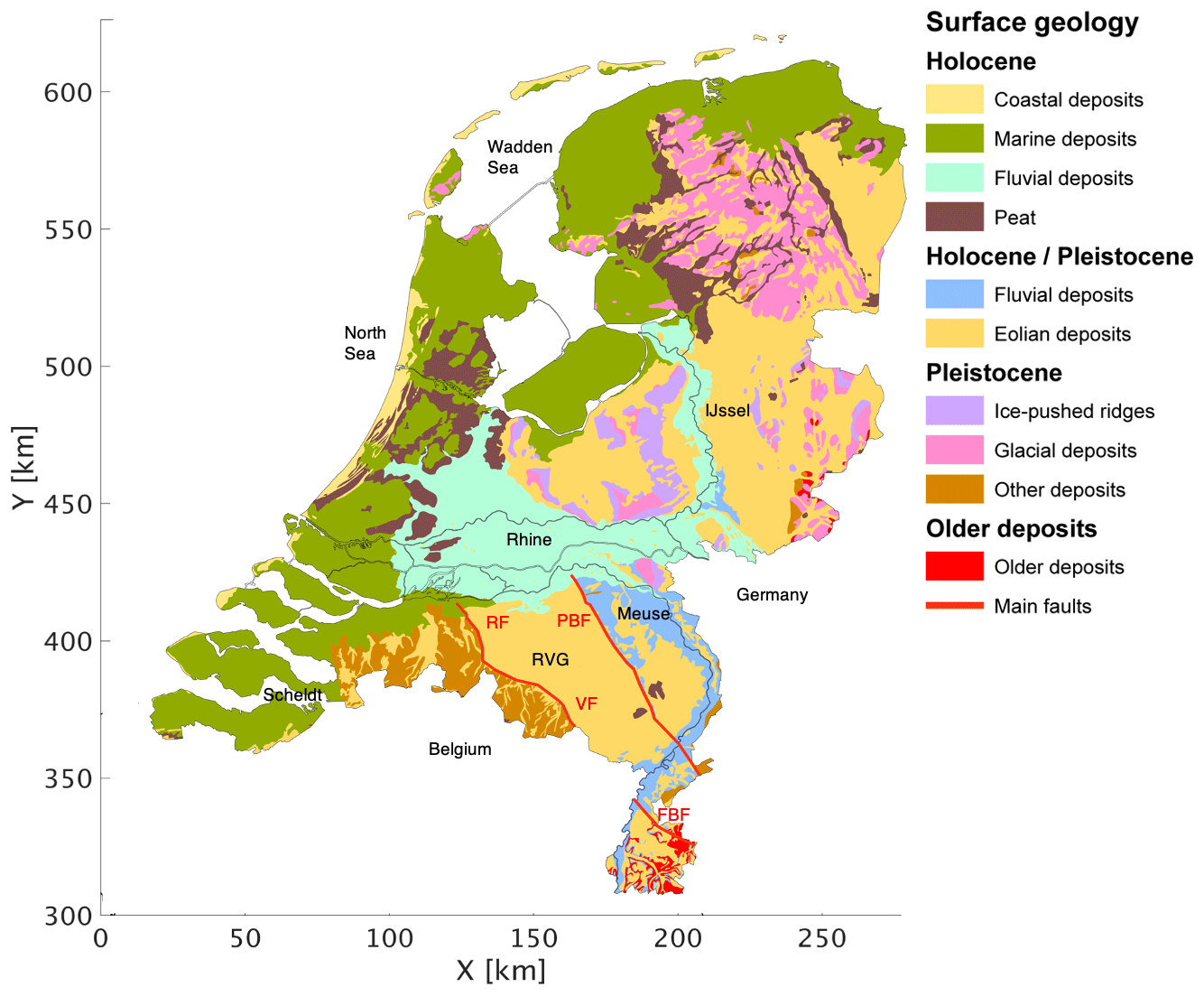
Figure 1 Surface geological map of the Netherlands. Older deposits comprise unconsolidated Neogene and Paleogene deposits as well as Mesozoic and Carboniferous limestones, sandstones, and shales. Modified after Schokker (2010). RF: Rijen Fault; VF: Veldhoven Fault; PBF: Peel Boundary Fault; FBF: Feldbiss Fault; RVG: Roer Valley Graben.

The Paleogene and Neogene sediments are dominated by marine clays and sands that were primarily deposited in shallow marine environments. The Quaternary sediments, reaching a maximum onshore thickness of ∼600 m, reflect a transition from shallow marine to fluvio-deltaic and fluvial depositional environments in the early Quaternary to a complex alternation of shallow marine, estuarine, and fluvial sediments in the younger periods (Zagwijn, 1989; Rondeel et al., 1996; De Gans, 2007; Busschers et al., 2007; Peeters et al., 2016). Imprints of glacial conditions are recorded in the upper part of the basin fill by, among others, deep erosive structures (subglacial valleys, tongue basins) and glacial till (Van den Berg and Beets, 1987).

2.1 Surface geology

The surface geology (Fig. 1) is mainly characterised by a Holocene coastal barrier and coastal plain in the west and north and an interior zone with Pleistocene deposits cut by a Holocene fluvial system (Rondeel et al., 1996; Beets and van der Spek, 2000). The coastal barrier consists of sandy shoreface and dune deposits and is up to 10 km wide. It is intersected in the south by the estuary of the Rhine, Meuse, and Scheldt and in the north by the tidal inlets of the Wadden Sea. The coastal plain is formed by mainly marine clay as well as peat. Although much of the peat has disappeared because of mining and drainage, thick sequences of peat (> 6 m) still occur. The Holocene fluvial deposits of the rivers Rhine and Meuse are characterised by a complex of sandy channel belt systems embedded in flood basin clays (Gouw and Erkens, 2007). The fluvial channel belts pass downstream into sandy tidal channel systems in the coastal plain (Hijma et al., 2009).

The Pleistocene interior of the country mainly consists of glacial, aeolian, and fluvial deposits (Rondeel et al., 1996; Van den Berg and Beets, 1987). Glacial deposits include coarsely grained meltwater sands and tills. Ice-pushed ridges, with heights up to 100 m, occur in the middle and east of the country. Aeolian deposits mainly consist of cover sands and are locally made up by drift sand and inland dunes. In the south and east of the country, sandy channel and clayey flood basin deposits of small rivers occur.

Neogene and older deposits are only exposed in the eastern- and southernmost areas of the country. In the east, these sediments include unconsolidated Paleogene formations as well as Mesozoic limestones, sandstones, and shales. In the south, the older deposits comprise unconsolidated Neogene and Paleogene sands and clays, as well as Cretaceous limestones (chalk), sandstones and shales, and Carboniferous sandstones and shales.

Figure 2 Map of the Netherlands depicting epicentres of all induced (M_w 0.5–3.6, orange) and tectonic (M_w 0.5–5.8, yellow) earthquakes from 1910–2020. The diameter of the circles indicates the relative earthquake magnitude. The triangles represent the surface location of the borehole stations (blue), borehole stations with SCPT measurements (purple), and single surface seismometers (green). The triangles with red outlines depict the locations of example HVSR curves presented in Fig. 8. The inset in the northeast depicts the location of the Groningen borehole network (G-network). Here, the red triangle depicts the location of borehole G24. The 19 (M_w≥2) induced earthquakes in this panel are used for the AF and ETF computations. Coordinates are shown within the Dutch national triangulation grid (Rijksdriehoekstelsel or RD), and lat–long coordinates are added in the corners for international referencing.

2.2 Regional seismicity

The Netherlands experiences tectonically related earthquake activity in the southeast, and induced earthquakes occur in the north at shallow depths due to exploitation of gas fields. Tectonic seismicity occurs mainly in the Roer Valley Graben (yellow circles, Fig. 2), which is part of a larger basin and range system in western Europe, the Rhine Graben Rift System. At the beginning of the Quaternary, the subsidence rate in the Roer Valley Graben did increase significantly (Geluk et al., 1995; Houtgast and Van Balen, 2000), and the rift system still shows active extension (Hinzen et al., 2020). The largest earthquake recorded (M_w=5.8) in the Netherlands was in Roermond in 1992, due to extensional activity along the Peel Boundary Fault (Paulssen et al., 1992). Gariel et al. (1995) quantified the near-surface amplification based on spectral ratios of aftershocks from the 1992 earthquake in Roermond. They observed great variety in ground motion amplitudes over different stations, which is the site effect of shallow sedimentary deposits.

Most induced earthquakes in the Netherlands (orange circles, Fig. 2) have their epicentre in the Groningen region due to production of the gas field. Here, reservoir compaction due to pressure depletion has reactivated the existing normal fault system that traverses the reservoir layer throughout the whole field. (Buijze et al., 2017; Bourne et al., 2014). Even though the magnitudes are relatively low (van Thienen-Visser and Breunese, 2015), the damage to buildings in the area is substantial due to shallow hypocentres and amplification on the soft near-surface soils (Bommer et al., 2017; Kruiver et al., 2017a).

3 Dataset

For this study, we use the seismic network of the Royal Netherlands Meteorological Institute (KNMI, 1993), consisting of borehole and surface seismometers distributed over the Netherlands (Fig. 2). The network includes 88 locations with vertical borehole arrays where each station is equipped with three-component 4.5 Hz seismometers at 50 m depth intervals (50, 100, 150, 200 m) and an accelerometer at the surface. The southernmost station is at Terziet (TERZ). This station consists of a borehole seismometer at 250 m depth and a surface seismometer. In Groningen, multiple boreholes have seismic cone penetration tests (SCPTs) taken directly adjacent to the borehole. The remaining triangles represent 29 locations of single surface seismometers (accelerometers and broad bands). All seismometers have three components and are continuously recording the ambient seismic field and, when present, local earthquakes. In Sect. 4 we use 19 local earthquakes of M≥2, recorded in the Groningen borehole network between May 2015 and May 2019. All data are available through the KNMI data portal (http://rdsa.knmi.nl/network/NL/, last access: 1 June 2021).

In the construction of the site-response map, we have made extensive use of the detailed 3D geological subsurface models GeoTOP and NL3D. Both models are developed and maintained by TNO – Geological Survey of the Netherlands (van der Meulen et al., 2013). GeoTOP schematises the shallow subsurface of the Netherlands in a regular grid of rectangular blocks (voxels, tiles, or 3D grid cells), each measuring 100 m by 100 m by 0.5 m (x ,y, z) up to a depth of 50 m below ordnance datum (Stafleu et al., 2011, 2021). Each voxel contains multiple properties that describe the geometry of lithostratigraphic units (formations, members, and beds), the spatial variation in lithology, and sand grain size within these units as well as measures of model uncertainty. GeoTOP is publicly available from the TNO's web portal: https://www.dinoloket.nl/en/subsurface-models (last access: 1 August 2021). To date, the GeoTOP model covers about 70 % of the country (including inland waters such as the Wadden Sea). For the missing areas we have used the lower-resolution voxel model NL3D, which is available for the entire country (van der Meulen et al., 2013). NL3D models lithology and sand grain-size classes within the geological units of the layer-based subsurface model DGM (Gunnink et al., 2013) in voxels measuring 250 m by 250 m by 1 m (x, y, z) up to a depth of 50 m below ordnance datum. To determine the depth of bedrock in the shallow subsurface, we consulted the layer-based subsurface models DGM and DGM-deep. These models are also available from the web portal mentioned above. More details on the models GeoTOP and NL3D are given in Appendix B.

4 Empirical relationships from the Groningen borehole network

The dense Groningen borehole network (G-network) provides the opportunity to derive empirical relationships between measured amplification in the time and frequency domain, estimated amplification from ambient vibrations, and the local lithostratigraphic conditions. First, we present results of three different methods to assess amplification. Next, we compare subsurface parameters with the measured amplification in order to evaluate which parameters are most critical.

4.1 Definition of amplification

The majority of site-response studies define the level of soft sediment amplification with respect to the surface seismic response of a nearby outcropping hard rock. In the Netherlands, no representative seismic response of outcropping bedrock is available. As an alternative, we define reference conditions as found in Groningen at 200 m depth, where we have many seismic recordings. These same reference conditions can be found at this depth over most locations in the Netherlands, though it can sometimes be deeper or shallower than 200 m. The corresponding elastic properties (shear-wave velocity and density) form the basis from which the ground motion amplification effect of any site with respect to the reference can be predicted. This approach is akin to the reference velocity profile that is used in Switzerland (Poggi et al., 2011).

For a recording at the Earth's surface, the upward and downward waves are simultaneously recorded, which leads to an amplitude doubling. This is called the free-surface effect. If the amplification is defined with respect to a surface (hard-rock) site, both the site of investigation and the reference site experience the same free-surface effect, and there is no need to remove it in order to isolate the relative amplification. We have a reference site at depth, where no free-surface effect takes place. Hence, we need to remove the free-surface effect first from the surface recording before isolating the relative amplification.

The G-network forms a representative resource for the definition of the reference horizon parameters. Hofman et al. (2017) and Kruiver et al. (2017a) determined shear-wave velocities at all borehole seismometer levels in Groningen. From their velocities found at 200 m depth, the average is taken, resulting in a reference shear-wave velocity of 500 m/s. At this depth, the sediment density is on average 2.0 kg/m³. At 200 m depth, 95 % of the Dutch subsurface is composed of laterally extensive Pleistocene and Pliocene sediments; hence the estimated site-response and corresponding amplification factors can be applied to a large part of the country. The remaining 5 % consists of shallow (<100 m) Triassic, Cretaceous, and locally Carboniferous bedrock, and therefore these locations need to be evaluated separately.

Frequency bandwidth

Data processing is applied to a frequency band-pass filter for 1–10 Hz, covering the periods of interest from an earthquake engineering point of view. Moreover, for these frequencies, the used instrumentation (broadband seismometers, accelerometers, and geophones) has high sensitivity for ground motion.

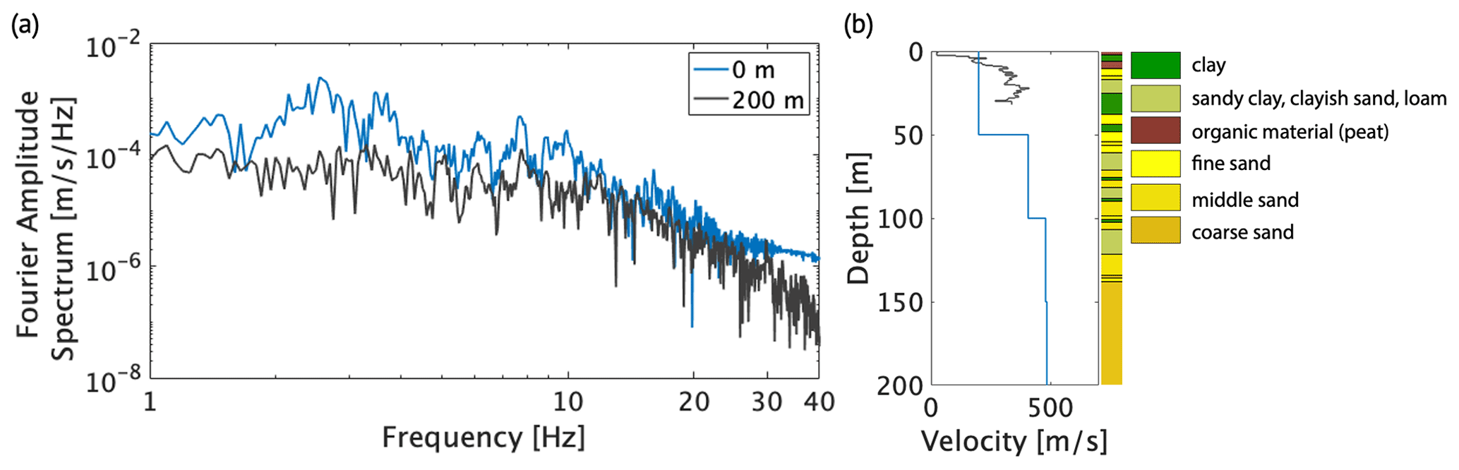
Figure 3 (a) Particle velocity Fourier amplitude spectrum measured on the radial component for the 200 m (grey) and surface seismometer (blue) for borehole G24 for a 20 s time window of the 8 January 2018 Zeerijp M 3.4 earthquake. Borehole G24 has an epicentral distance of 10 km. (b) Shear-wave velocity profile for G24 with the interval velocities from Hofman et al. (2017) in blue and the shear-wave velocity from the adjacent SCPT over the top 30 m (black line). The corresponding lithological profile is derived from GeoTOP (https://www.dinoloket.nl/en/subsurface-models, last access: 15 October 2021).

Since most of the amplification is occurring in the top sedimentary layer (van Ginkel et al., 2019), the corresponding resonance frequencies are covered in the used frequency filter as well. Above 10 Hz, the amplitude increase due to soil softening and resonance is counteracted by an elastic attenuation and 3D scattering. Furthermore, what exactly happens above 10 Hz is of little interest since most of the local earthquake energy is contained in the frequency band between 1 and 10 Hz. This is illustrated in Fig. 3, which presents the particle velocity Fourier amplitude spectrum of a local earthquake recorded in borehole G24. The location of this borehole is presented as a red triangle in Fig. 2.

4.2 Amplification factors

We compute an overall amplification factor from the G-network earthquake recordings by taking the ratio of the maximum amplitudes recorded at the surface and the 200 m deep seismometer, following the procedure described in van Ginkel et al. (2019). This ratio is taken for both the radial (R) and transverse (T) components, and the results are averaged. The amplitude at the surface is divided by a factor of 2 in order to remove the effect of the upward and downward waves recorded at the same time. Earthquake records are processed in the time domain for a 20 s time window and frequency band of 1–10 Hz. Next, the AF for each borehole is obtained by repeating the above procedure for 19 available M≥2.0 local induced earthquakes and subsequently averaging the values. It is determined in the time domain and therewith provides an average amplification over the applied frequency band.

Many studies (e.g. Bommer et al., 2017; Rodriguez-Marek et al., 2017; Borcherdt, 1994) model site-response amplification factors (AFs) for different periods of spectral accelerations, which tailors to engineering structures with different resonance frequencies. In this study we aim to provide an average amplification level in a broad frequency band. The choice for the specific AF frequency band was supported by evaluating amplification over a range of frequency bands. Figure 4 shows the AFs over the Groningen network for several bands. AF values are highest in the band 1–5 Hz due to the strong resonances of the Holocene infill (van Ginkel et al., 2019). In the 1–10 Hz band the AFs are lower but contain considerable earthquake amplitudes (Fig. 3). When the frequency band is extended beyond 10 Hz (Fig. 4c and d), the AF values do not change significantly. We decided to pick the frequency band of 1–10 Hz as the representative AF since it is a better overall representation of amplification by the soft sediments than the higher values of 1–5 Hz, as shown in Wassing et al. (2012).

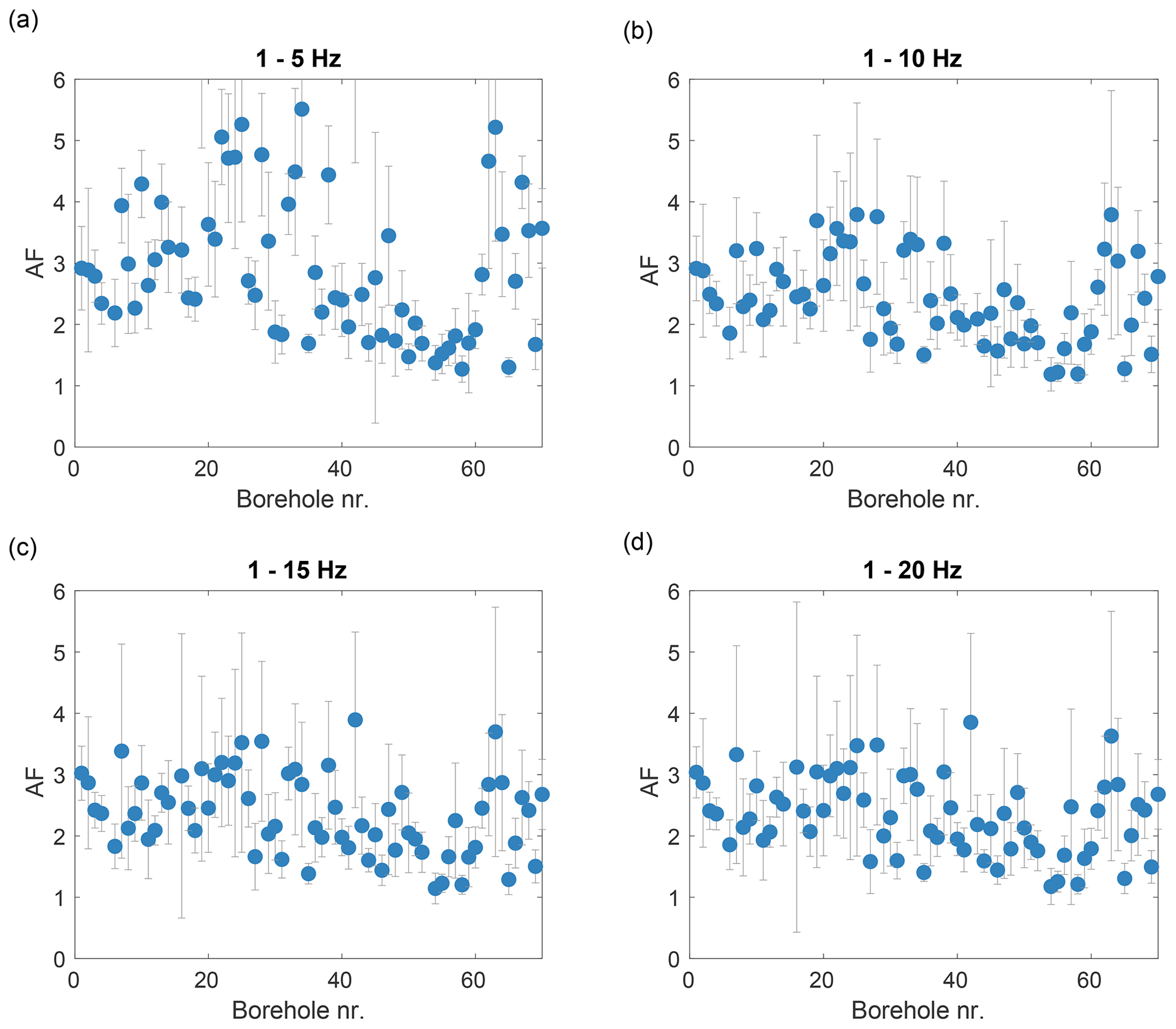
Figure 4 Amplification factors (AFs) for (a) frequency bands 1–5 Hz, (b) 1–10 Hz, (c) 1–15 Hz, and (d) 1–20 Hz and corresponding standard deviations (error bars) associated with the averaged AFs over 19 M≥2.0 local earthquakes.

4.3 Empirical transfer functions

Empirical transfer functions (ETFs) represent shear-wave amplification in the frequency domain. ETFs are defined as a division of the Fourier amplitude spectra at two different depth levels. With a reference horizon at 200 m depth and the level of interest at the Earth's surface, the transfer function has both a causal and acausal part. The causal part maps upward-propagating waves, from the reference level to the surface. The acausal part maps downward-propagating waves back to the free surface (Nakata et al., 2013). When describing amplification, we are only interested in the causal part. We select this causal part of the estimated transfer function and compute its Fourier amplitude spectrum to obtain a measure of frequency-dependent amplification. We use 20 s long time windows for particle velocity recordings on the radial component of the G-network seismometers. Subsequently, we average over 19 local earthquakes with magnitudes ≥2.0. This can be seen as an implementation of seismic interferometry by deconvolution (Wapenaar et al., 2010). Lastly, the deconvolution results are stacked to enhance stationary contributions.

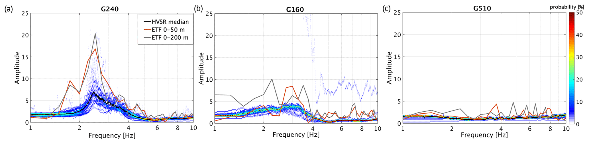
Figure 5 Probability density function of 1 month of daily HVSRs and the mean HVSR (solid black line) and ETF for the borehole seismometer interval of 0–50 m (grey dashed line) and 0–200 m (grey solid line). The selected borehole sites exhibit differences in curve characteristics with (a) G24 illustrating clearly peaked curves (>4), (b) G16 illustrating medium (2–4) peak amplitudes, and (c) G51 with no pronounced peak.

From the ETF between the 200 m depth and surface seismometer (ETF₂₀₀), peak amplitudes are identified. Some example ETF curves are plotted in Fig. 5. Additionally, ETF curves for the top 50 m are calculated (ETF₅₀). The ETF curves for the different intervals show very similar peak characteristics and peak amplitudes, demonstrating that most amplifications are developed in the top 50 m of the sediment cover. Furthermore, the borehole sites with the highest ETF peak amplitudes can be linked to the local geology, as presented in van Ginkel et al. (2019, Fig. 9). Here, highest peak amplitudes are measured at sites with unconsolidated Holocene alternations of clay and peat, overlying consolidated Pleistocene sediments.

4.4 $H/V$ spectral ratios from the ambient seismic field

The Groningen surface seismometers are continuously recording the ambient seismic field (ASF), and these data are used to estimate horizontal-to-vertical spectral ratios (HVSR). In this study we focus on the second peak (≥ 1 Hz) in the HVSR curve, which represents shear-wave resonances at the shallowest interface of soft sediments on top of more consolidated sediments. Resonances of the complete sediment layer display a peak at lower frequencies (van Ginkel et al., 2020). Above 1 Hz the noise field is dominated by anthropogenic sources. The details of the method to obtain stable HVSR curves from the ASF in the Groningen borehole network can be found in van Ginkel et al. (2020). In summary, from power spectral densities for each component, the $H/V$ division is performed for each day. Subsequently, a probability density function is computed over one month of $H/V$ ratios and the mean is extracted. This yields a stable HVSR curve that is not much affected by transients like nearby footsteps or traffic.

Based on the HVSR curve and peak characteristics, different criteria are defined conformable to the SESAME consensus (Bard, 2002): (1) clear peaked curves (HVSR amplitude >4) related to a sharp velocity contrast in the shallow subsurface. (2) HVSR peak amplitude between 2–4, associated with a weak velocity contrast. (3) No distinguishable peak and a flat curve indicate the absence of a velocity contrast in the shallow subsurface. Example HVSRs for these three criteria are plotted in Fig. 5. Its associated peak amplitudes are derived from the mean HVSR curve and presented in van Ginkel et al. (2019). The correlation between peaks on the HVSR curves and the presence of a velocity contrast at some depth is stressed in studies from Bonnefoy-Claudet et al. (2008), Konno and Ohmachi (1998) and Lermo and Chavez-Garcia (1993) and this contrast is very likely to amplify the ground motion.

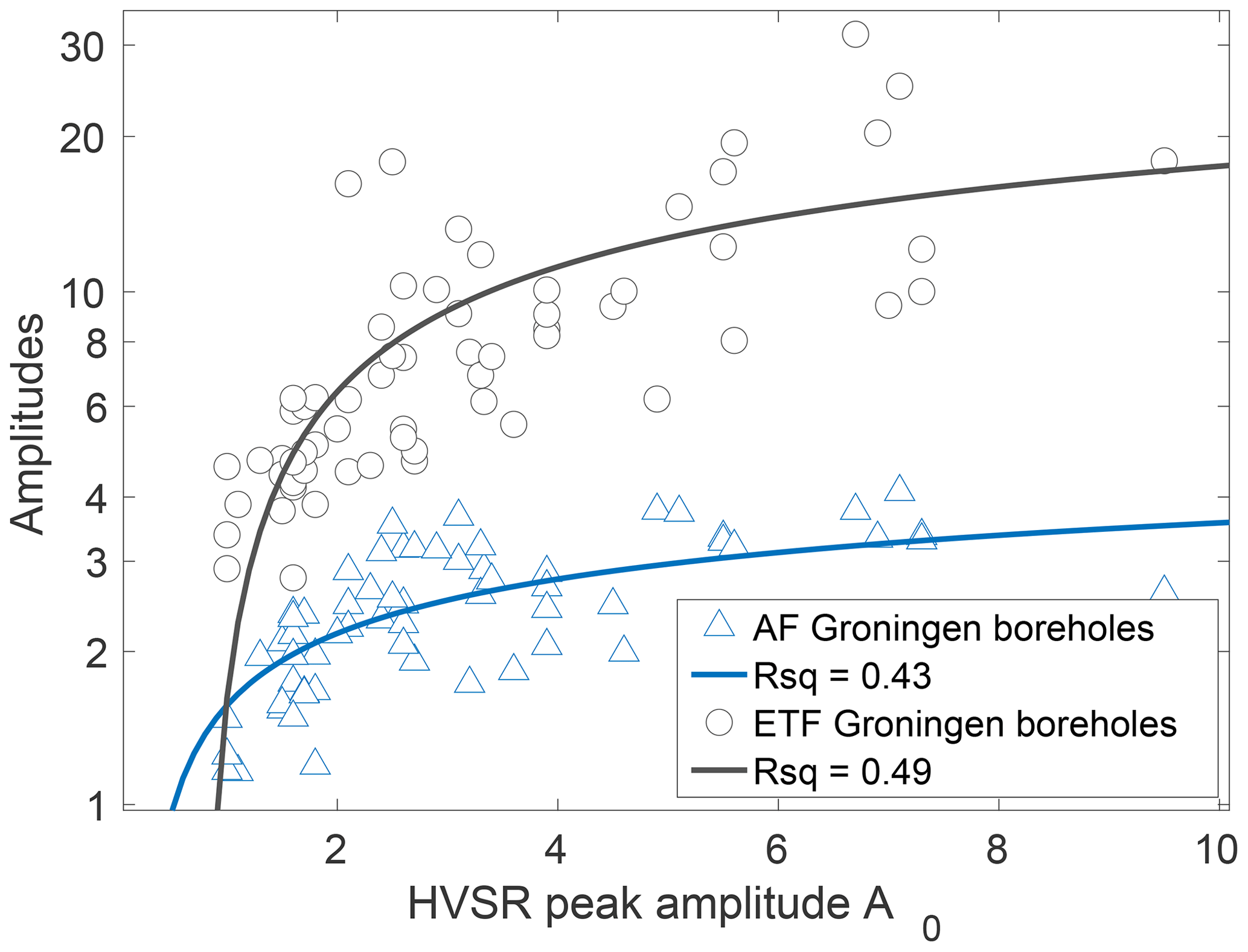
Figure 6 Relation between the HVSR peak amplitudes (A₀) and the ETF peak amplitudes (grey) and the HVSR peak amplitudes and the AF (blue). The solid line represents the fitting function (Eqs. 1 and 2) between the HVSR peak amplitudes and the measured amplification from AF and ETF, respectively. R_sq (R-squared) represents the coefficient of determination of the fitting. Note the log-scale of the y axis.

4.5 Amplification parameters

Across the Netherlands, the ASF is continuously recorded on all seismometers, while many locations lack recordings of local earthquakes. Therefore we further investigate whether the HVSR can be used as a proxy for amplification as measured by the earthquake-derived ETF and AF. Figure 6 displays the correlation between the peak amplitudes of the HVSR and ETF₂₀₀ as well as HVSR and AF. Secondly, we evaluate the subsurface seismic parameters enhancing amplification (Fig. 7).

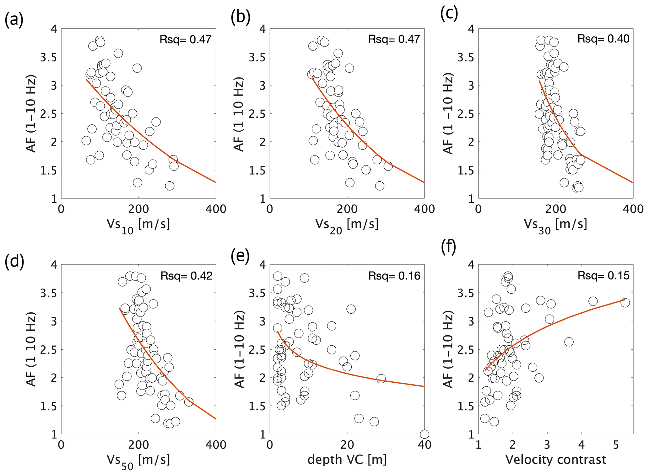
Figure 7 Each panel depicts the fitted function and the coefficient of determination (R_sq) of the AF (1–10 Hz) per G-network borehole location and the corresponding subsurface parameter. (a) V_s10, (b) V_s20, (c) V_s30, (d) V_s50, (e) depth of the velocity contrast, and (f) size of the velocity contrast.

Based on these data points, relationships are defined in order to be able to estimate amplification factors using HVSR peak amplitudes (A₀), amplification factors:

$$\begin{array}{}\text{(1)}& \text{AF}=\mathrm{1.49}+\mathrm{0.87}\log \left(\mathrm{1.12}{A}_{\mathrm{0}}\right),\end{array}$$

and maximum amplification as measured by the ETF:

$$\begin{array}{}\text{(2)}& \text{ETF}=\mathrm{1.08}+\mathrm{6.89}\log \left(\mathrm{1.09}{A}_{\mathrm{0}}\right).\end{array}$$

The relationship between the AF derived from the Groningen borehole locations and local site conditions is investigated in the following.

Many ground motion prediction equations which include site response consider the shear-wave velocity for the top 30 m (V_s30) as the main parameter affecting amplification (Akkar et al., 2014; Bindi et al., 2014; Kruiver et al., 2017b; Wills et al., 2000), as well as Eurocode 8 (Comité Européen de Normalisation, 2004). However, studies (Castellaro et al., 2008; Kokusho and Sato, 2008; Lee and Trifunac, 2010) have drawn attention to the fact that using only V_s30 as a proxy for site response is inadequate, because it does not uniquely correlate with amplification. They show that amplification is defined by several parameters, including the depth and degree of the seismic impedance contrast. Furthermore Joyner and Boore (1981) introduce the shear-wave velocity ratio between the top and base layers as a proxy for site amplification, and this is further explored by Boore (2003).

In order to assess the impact of different parameters, firstly, the AF at each borehole location is fitted against several subsurface parameters. $\text{AF}=a+b\cdot e^{c\cdot V_{\mathrm{s}}}$ as a functional form, where a, b, and c are unknown coefficients to be fitted. This fitting is applied with averaged shear-wave velocities over various depth intervals. V_s10, V_s20, and V_s30-values are derived from SCPTs, acquired directly adjacent to 53 borehole sites in Groningen (Fig. 2). Hofman et al. (2017) derived interval velocities determined from the G-network, using seismic interferometry applied to local induced events. The velocities from this reference are used to determine V_s50. Secondly, from the SCPT data we derive the depth and size of the velocity contrast. The contrast is computed by the division of the two different velocity values bounding each 1 m interval. This division is done for each 1 m interval over the 30 m of SCPT records. The largest division value is defined as the (main) velocity contrast (VC), and corresponding depth is the depth of the contrast (zVC). Thereafter the VC values and their depth are fitted with the AF using $\text{AF}=a+b\cdot \log (c\cdot \text{VC})$ as a functional form. This procedure is also performed for the relation between the subsurface parameters (V_s, VC) and the HVSR. The results are given in Appendix A.

Figure 7 presents the fit between the AF and the six relevant subsurface parameters. Best fit (R_sq=0.47, Fig. 7a and b) is observed between the AF and V_s10 and V_s20. This is in line with findings of Gallipoli and Mucciarelli (2009), who use the V_s10 as the main amplification parameter instead of the more common V_s30. In Groningen, the low-velocity and unconsolidated Holocene sediments have a thickness of 1 to 25 m, and below these depths the velocities increase in the more compacted Pleistocene sediments. The reduced fitting quality of V_s30 and V_s50 arises since the amplification develops mainly in the Holocene sediments (van Ginkel et al., 2019). Although the fit is relatively poor, a relationship is observable between a large VC and an elevated AF (Fig. 7e). By contrast, Fig. A1 presents a good correlation between VC and HVSR. A large VC value leads to resonance in the near surface, which is expressed in high-amplitude peaks of the HVSR.

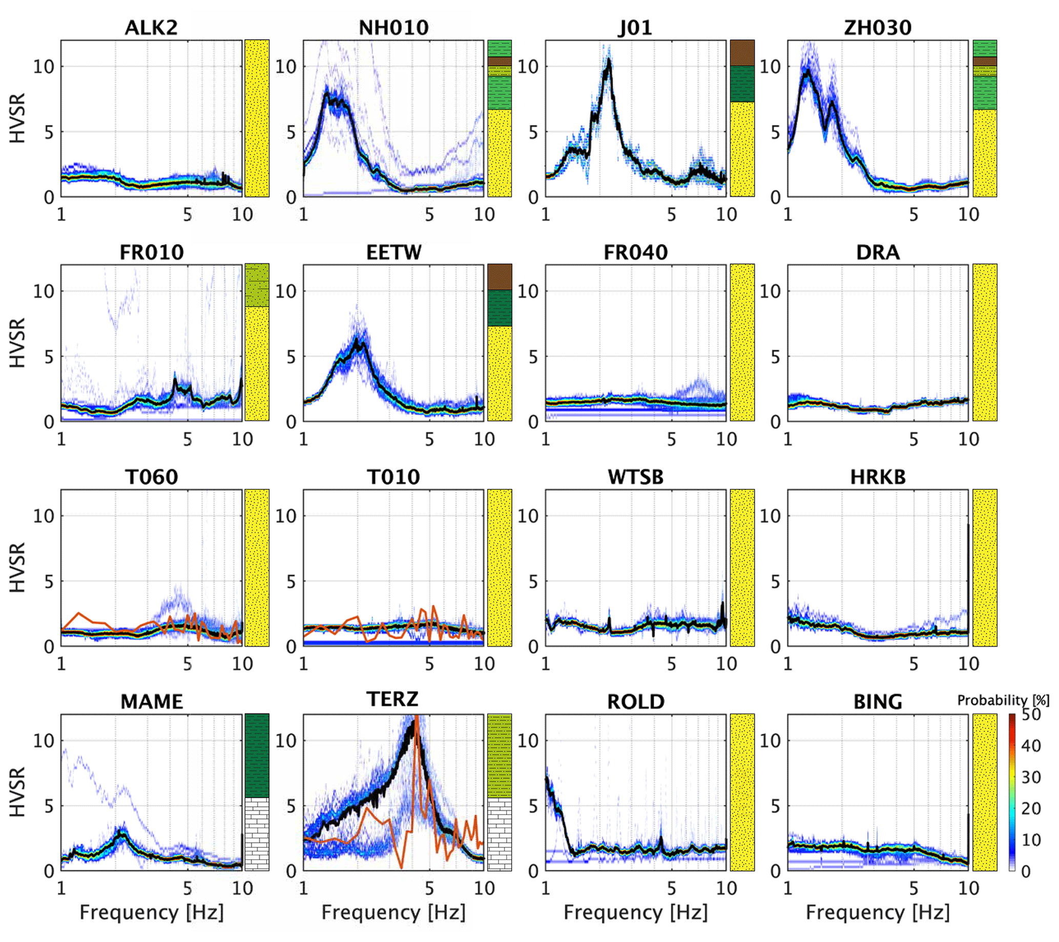
Figure 8 Each panel depicts a probability density function from ambient noise HVSR curves and sediment classification profile (Sect. 6) for 16 stations of the NL network. The black line represents the mean HVSR, and the red line in the panels of T06, T010, and TERZ represents the ETF calculated from 10 local earthquakes. The colour bar in the lower right displays the HVSR probability range that is valid for all panels.

5 HVSR estimations throughout the Netherlands

Based on the good relationship between Groningen HVSR peak amplitudes (A₀), ETF peak amplitudes, and AF (Fig. 6), we conclude that the HVSR can be further used as proxy for amplification. Therefore, for all surface seismometers in the Netherlands seismic network, the HVSR curves are estimated following the method described in Sect. 4.4. Figure 8 displays a selection of representative examples of HVSR curves. It also includes the sediment classification profile presented in Sect. 6 and Fig. 9. In addition, for boreholes T010, T060, and TERZ, the ETF curve is added, calculated from local earthquakes similar to the approach described in Sect. 4.3. These 16 HVSR curves illustrate the diversity in curve characteristics throughout the Netherlands. Here, we can distinguish the three types of curves as described in Sect. 4.4. The flat curves with no distinguishable peak (FR040, DRA, T060, T010, WTSB, HRKB, ROLD, and BING) are recorded at seismometers on top of outcropping Pleistocene sands (Holocene–Pleistocene aeolian and fluvial deposits in Fig. 1). Also, ALK2 exhibits no peak amplitude since this seismometer is positioned on dune sands (Holocene coastal deposits in Fig. 1). These locations are characterised by absence of a strong velocity contrast in the shallow subsurface. Selected examples of HVSR curves exhibiting clear peak amplitudes (NH01,J01, ZH030, FR010, EETW) are located at sites with a distinct velocity contrast between unconsolidated Holocene marine sediments overlying Pleistocene sediments.

In the southernmost part of the Netherlands, Cretaceous bedrock is either outcropping or situated less than 100 m deep. MAME and TERZ are examples of locations with soft sediments overlying hard rock, and the HVSR curves exhibit a clear peak amplitude.

6 Zonation map for the Netherlands

The effect of local site response on earthquake ground motion is included in the Eurocode 8 seismic design of buildings (Comité Européen de Normalisation, 2004, EC8). In order to estimate the risk of enhanced site response, EC8 presents five soil types based on shear-wave velocities and stratigraphic profiles. Soil type E is essentially characterised by a sharp contrast of a soft layer overlying a stiffer one. However, in our opinion, this single classification for soft sediments is rather limited, especially concerning the wide variety of lithostratigraphic conditions throughout the Netherlands. Therefore, we present an alternative, or extended, classification for ground characteristics designed to specify the large heterogeneity in site conditions than exists within Eurocode 8 ground type E.

In this section, in a few steps, the site-response zonation map for the Netherlands is derived. For this, the country is subdivided into grid cells. As a result, about 95 % of the grid cells are populated with a site-response class with a corresponding AF.

6.1 Classification scheme

The borehole ETFs confirm that most of the amplification is developed in the top 50 m (Fig. 5) of the sedimentary cover, corresponding to the findings in van Ginkel et al. (2019). Beyond 50 m depth, the Quaternary deposits mainly consist of more compacted marine and fluvial sediments. Therefore the sediment classification presented in this section uses the top 50 m with a special focus on the top 10 m. Also, the presence of a velocity contrast is used in the classification, as it was shown to have a (albeit weaker) link with amplification (Figs. 7 and A1).

Table 1 Details of the NL classification. The V_s10 and velocity contrast (VC) values assigned to each class are based on the amplification relationships presented in Sect. 4 and Appendix A. For class V there are no empirical data available relating V_s10 and VC with A₀ (HVSR peak amplitude), hence not determined (n.d).

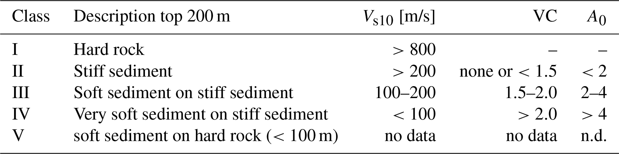
Following Convertito et al. (2010) and from the studies by Kruiver et al. (2017a) and van Ginkel et al. (2019), the Eurocode 8 classification requires modification, caused by the heterogeneous shallow sediment composition and bedrock depth of the Dutch subsurface. Table 1 lists the criteria for the classification division defined for the Netherlands (NL classification). The NL classification is divided into five classes based on the top 50 m lithostratigraphic composition, the velocity contrast (VC), and average shear-wave velocity for the top 10 m.

For setting up the classification, we initially use A₀, the peak amplitude from HVSR. We only have measured AF in Groningen, whereas we have measured A₀ for many sites throughout the Netherlands (all stations depicted in Fig. 2). Moreover, we found a clear relationship between A₀ and AF (Eq. 1). The relationships between V_s10, VC, and A₀ are estimated from lithological conditions in Groningen, where the sites are assigned to Classes II, III, and IV. For Classes I and V we have insufficient empirical constraint on A₀ and AF. Only sites with bedrock at depths shallower than 100 m fall into Class V, for which the resonance over the complete unconsolidated cover can reach frequencies larger than 1 Hz. Therewith, these sites become distinct from Classes II, III, and IV, where such resonances occur at frequencies <1 Hz. At these lower frequencies, there is no match with resonance periods of most building types in the Netherlands.

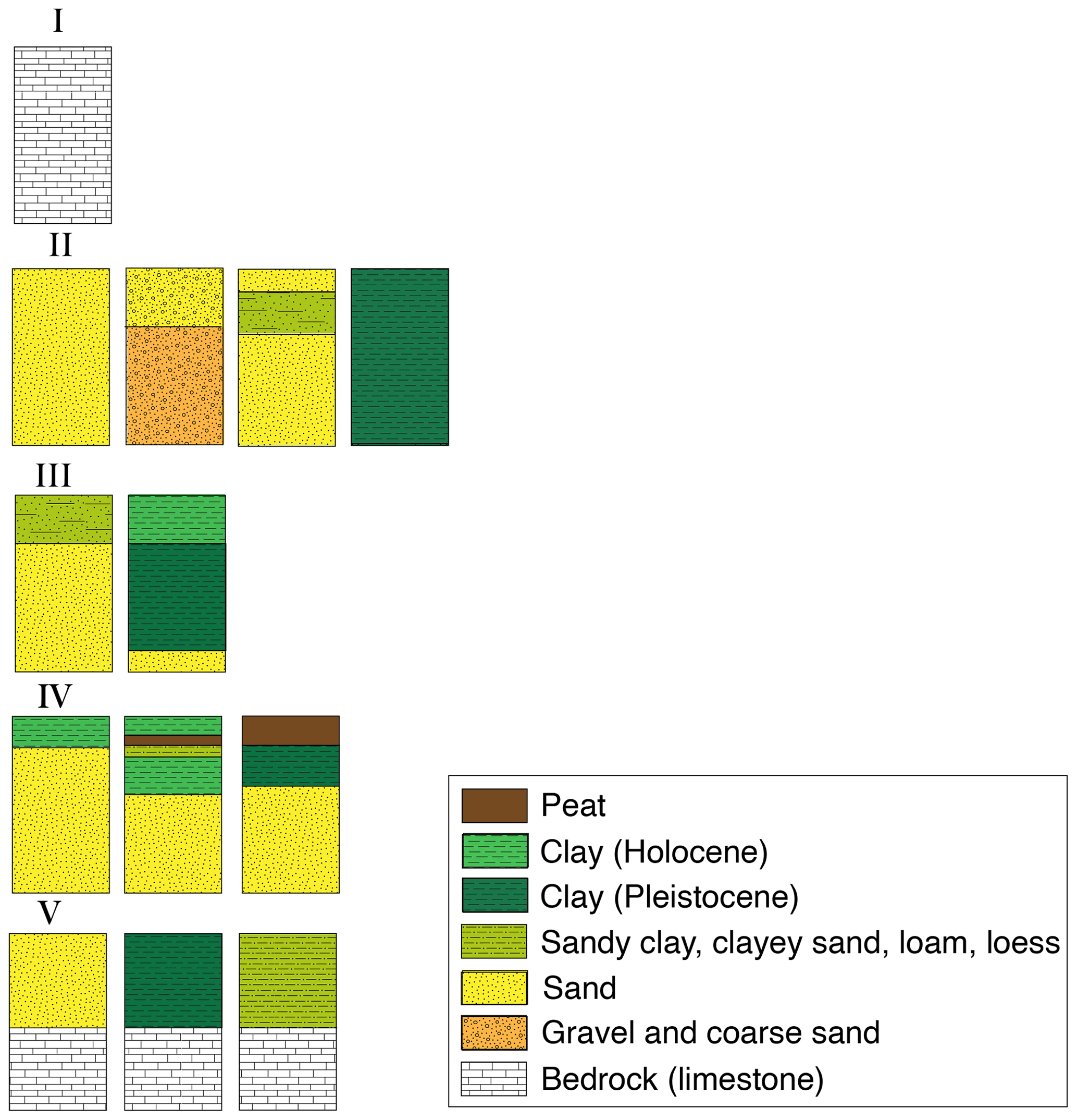
Figure 9 Sediment profiles corresponding to the classification presented in Table 1, where the different columns are typical examples of the top 50 m of the Netherlands. The division in classes is based on the shallow subsurface composition related to the expected level of wave amplification during a seismic event.

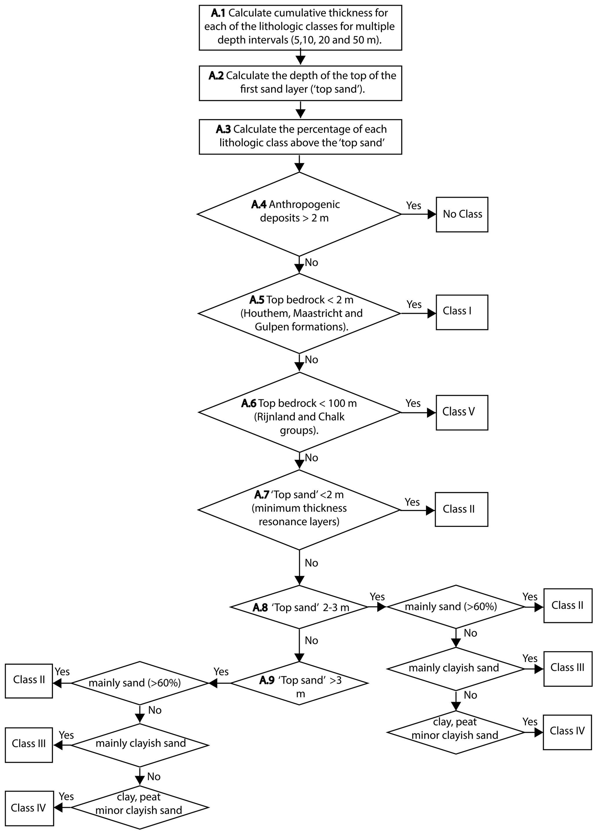
Figure 10 General outline of the vertical voxel-stack analysis used to assign the appropriate sediment class into each grid cell of the GeoTOP and NL3D geological models in the construction of the site-response zonation map.

The short lithological description in Table 1 is not sufficient to classify each site. To further aid the classification, representative sediment profiles are obtained (Fig. 9) based on the lithologic class sequences of the GeoTOP and NL3D. By grouping the main sediment profiles into the classes, we link the lithostratigraphic conditions to the expected amplification behaviour of the shallow subsurface. The classification is tested and optimised using all the sites with an estimated HVSR curve. The next step is to attribute a class to each lithostratigraphic profile per grid cell in the GeoTOP and NL3D models.

6.2 Lithology-based classification

Based on the site-response amplification estimated with the HVSR peak amplitudes at 115 sites, we have categorised each sedimentary profile (Fig. 9) into a class. The next step is to substitute GeoTOP and NL3D into these five classes. This geologically based method allows the determination of site response on regional and nationwide scales. Figure 10 gives a general outline of the procedure used to assign the appropriate sediment class to each of the voxel stacks in GeoTOP and NL3D. A voxel stack is the vertical sequence of voxels at a particular (x,y) location in GeoTOP or NL3D. Details on each of the processing steps are given in Appendix C. The next step is to attribute an amplification factor to each class.

6.3 Amplification factors for the Netherlands

For shake-map implementations or seismic hazard analysis, amplification factors (AFs) are usually derived from the V_s30 (e.g. Borcherdt, 1994). In this study, we estimate AFs by substituting the HVSR peak amplitudes (A₀) for 115 stations throughout the Netherlands into Eq. (1). This allows the calculation of nationwide applicable AF values (AF_NL) assigned to each of the classes presented in Fig. 9.

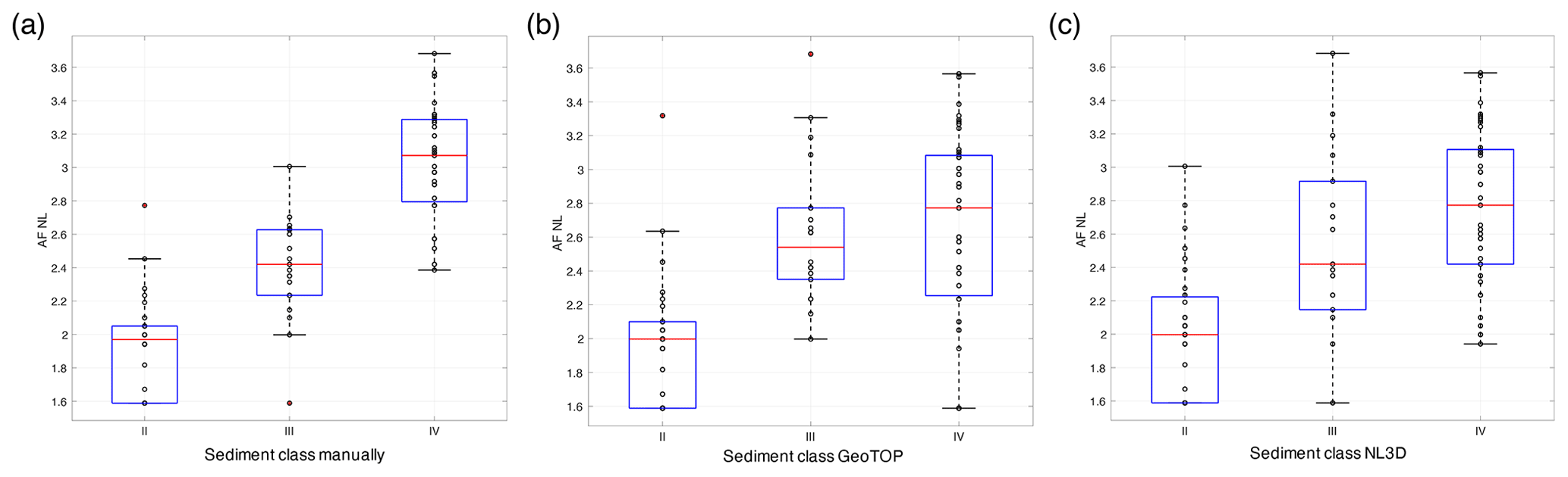
Figure 11 Comparison of calculated AF distribution in terms of manual classification (a) and automatic classification by GeoTOP (b) and by NL3D (c). The locations where the empirical AF relationship is not valid are eliminated (Classes I and V). The red central mark indicates the median; the bottom and top edges of the box indicate the 25th and 75th percentiles, respectively. The whiskers extend to the most extreme data points, and the outliers (1.5× away from the interquartile range) are plotted individually as red circles.

In order to obtain an AF_NL for each class, the 115 calculated AFs are plotted against their site sediment class in Fig. 11a. For these 115 locations, the sediment classes are manually assigned based on the geological models, SCPT, or other geological data available. From the AF distributions, the mean AF values (AF_NL) and corresponding standard deviation (σ_AF) are calculated for each class (Table 2). In Class II there are a number of sites with exactly the same AF of 1.6. These are sites with no distinguishable peak, where A₀ is set to 1, which yields, after filling out in Eq. (1), AF = 1.6.

The AF_NL values are valid on a national scale for a frequency range of 1–10 Hz and for reference conditions of V_s=500 m/s (Sect. 4.1). There are no AF values for sites in the farthest south and east of the Netherlands, so these areas fall into Classes I and V. There are too few data to calibrate the corresponding amplification factor.

By applying the workflow that we introduced in Sect. 6.2, automatic classification for the 115 sites is performed based on GeoTOP and NL3D and plotted against the AF (Fig. 11b and c). Due to uncertainties in the models (Appendix C), these distributions deviate from the manual classification (Fig. 11a). Note that for the manual classification SCPT information could be used at 53 sites for which local information is not included in GeoTOP and NL3D. We therefore distinguish two types of uncertainty.

1. σ_AF. This is the variability that originates from the classification. Within the classification, a number of different sites are binned into the same class (Fig. 9), although in reality there is still a range of amplification behaviour. This variability is approximated with the outcome of the manual classification (Fig. 11a), which could be done in great detail.

2. σ_mod. The geological models are geostatistical models where not all grid cells contain individual lithological data. Hence, there is an uncertainty of the actual lithological succession at each grid cell. The total uncertainty σ_tot (derived from Fig. 11b and c) can be written as $\sqrt{{\mathit{\sigma }}_{\mathrm{AF}}^{\mathrm{2}}+{\mathit{\sigma }}_{\mathrm{mod}}^{\mathrm{2}}}$. By additionally averaging over the classes (labelled with subscript _i), we find the model uncertainty σ_mod:

   $$\begin{array}{}\text{(3)}& {\mathit{\sigma }}_{\mathrm{mod}}={\displaystyle \frac{\mathrm{1}}{n}}\sum _{i=\mathrm{1}}^n\sqrt{{{\mathit{\sigma }}_{\mathrm{tot},i}}^{\mathrm{2}}-{{\mathit{\sigma }}_{\mathrm{AF},i}}^{\mathrm{2}}}.\end{array}$$

Table 2 lists the mean AF values, the uncertainty in AF (σ_AF), and the uncertainty (σ) for the GeoTOP and NL3D models.

6.4 Site-response zonation map

The workflow presented in Fig. 10 results in a class category assigned to each grid cell of the GeoTOP and NL3D models. As a result, we present the national site-response zonation map (Fig. 12), where each class characterises a certain level of expected site-response amplification. Additionally, each class has an AF_NL assigned (Table 1). Figure 13 presents four zoom-in panels of the map, each depicting a region of particular interest.

Table 2 Amplification factors and standard deviations (σ) for the NL classification. σ_AF is the uncertainty when a local (HVSR) recording is available. σ GeoTOP and σ NL3D represent the additional uncertainty associated with the GeoTOP and NL3D models.

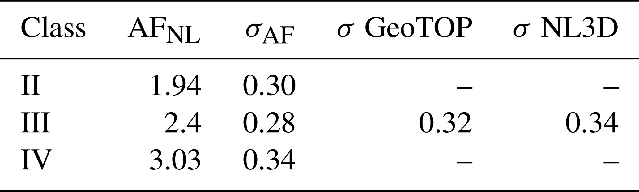
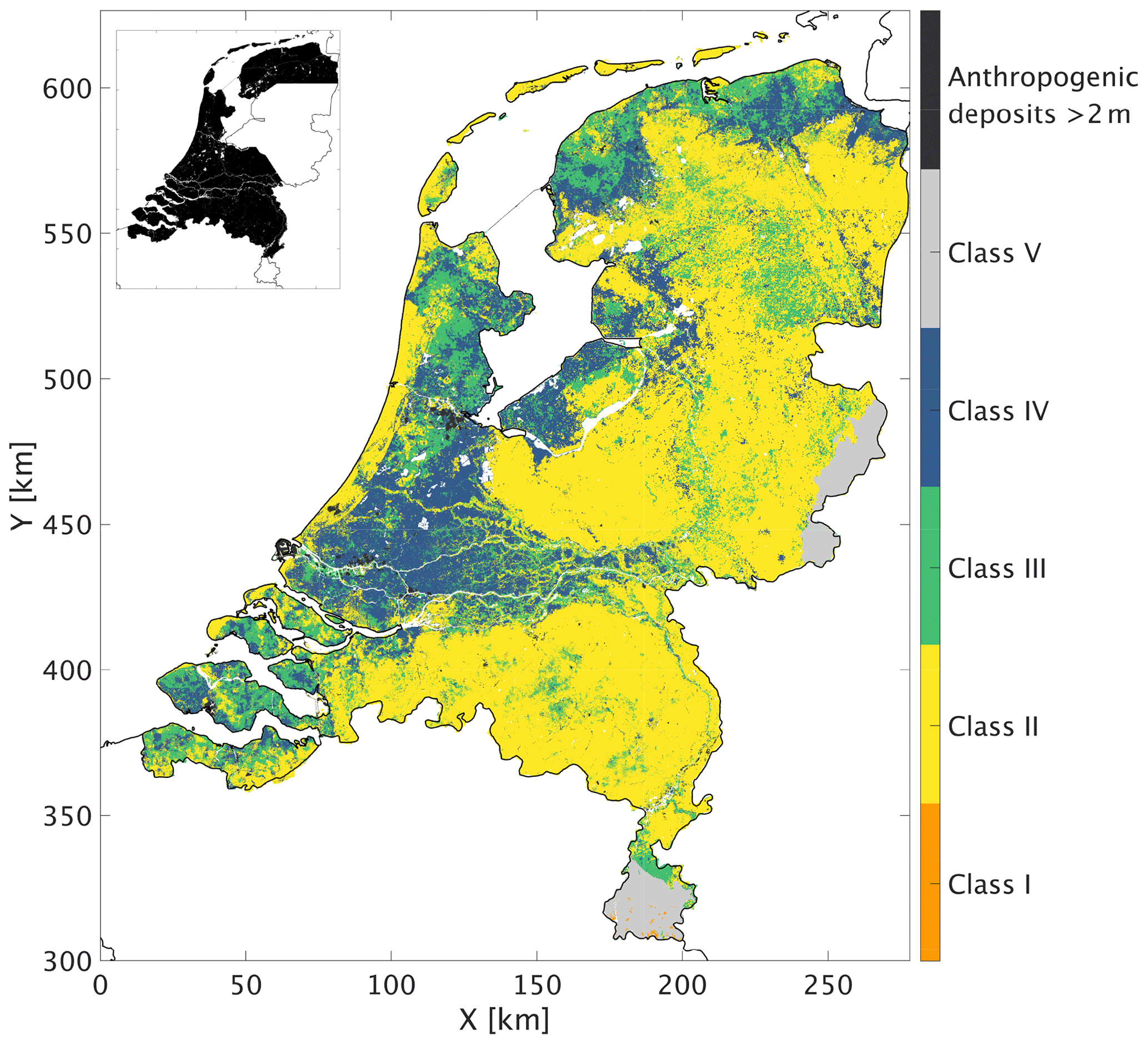
Figure 12 Seismic site-response zonation map for the Netherlands designed for low-magnitude induced earthquakes. The GeoTOP model coverage is highlighted in black in the small inset. For the remaining part of the Netherlands, the NL3D model is used as the foundation for the classification. The white spots are water bodies. The amplification factors and related uncertainties are presented in Table 2.

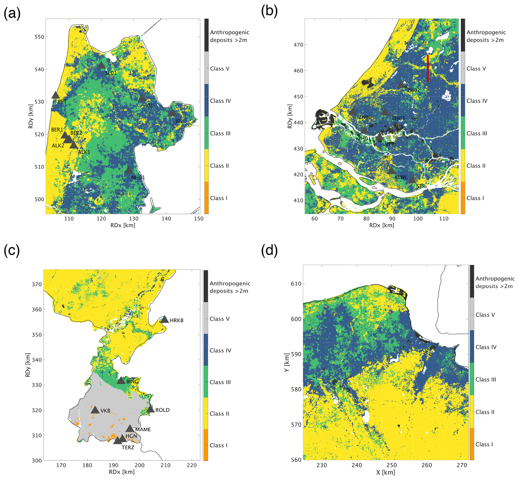
Figure 13 Panels highlighting different regions in the site-response zonation map, including the seismometer locations. (a) North Holland: with a heterogeneous pattern between Classes III and IV. (b) The densely urbanised area of South Holland: the red line indicates the S–N cross section through the GeoTOP voxel model (Fig. C1). (c) Limburg is in the north, a quite homogeneous zone of Class II, while the south is dominated by Classes I and V due to shallow and outcropping bedrock. (d) Northeast Groningen is added as a comparison to other studies performed in that region. No seismometer locations are plotted here because of the high density covering the map.

Some areas show a large scatter in classes, which is derived from a large heterogeneity in the near surface as represented in the lithostratigraphic models. Typically, at these places there is large model uncertainty, for example in northeast North Holland (Fig. 13a). Here, the Holocene lithological successions are very heterogeneous in terms of clay, peat, and clayish sand. This region also exhibits discrepancies between the model's lithological successions and HVSR curve characteristics, for instance with seismometers J01 (Fig. 8) and J02. The geological model at these locations presents large portions of clayish sand, resulting in Class III, while the HVSR curves exhibit distinctive, high-amplitude peaks, demonstrating local conditions related to Class IV.

For larger sedimentary bodies, like the dune area, there is less model uncertainty. Dune sand is identified as Class II, and here, the HVSR of the seismometers (e.g. ALK2, Fig. 8) lacks any peak due to the absence of a velocity contrast in the near surface.

Figure 13b covers the “Randstad” region, the most densely urbanised part of the Netherlands, where the class is mainly determined as IV. Figure 13c shows the southeastern part. Most of the northern part of this region is Class II due to Pleistocene sands reaching the surface. Most of the southern part of this region falls into Class V since the bedrock occurs at a depth less than 100 m. A few places with bedrock outcrops fall into Class I.

Since Groningen has been studied in much detail, we also present the site-response zonation for this region (Fig. 13d) and discuss this in Sect. 7.

7 Discussion

The seismic site-response zonation map presented in Fig. 12 distinguishes five classes, each of which defines the potential of occurrence of the related site-response amplification. Here, the lithological conditions are collated into zonations (classes) using the classification as shown in Fig. 9. In the development of the lithostratigraphically based classification, we used (i) HVSR peak amplitudes, (ii) the presence of a velocity contrast at depth, (iii) shear-wave velocities. Amplification factors are assigned to each class. In the following paragraphs we discuss the validity and uncertainties of the classification, the AF distributions, and the usage and limitations of the presented map.

Since the ambient noise sources in the frequency band of interest (1–10 Hz) partly have an anthropogenic origin, one should be careful about contamination by local strong noise because it may seriously affect the amplitude of the HVSR as shown in Guillier et al. (2007) and Molnar et al. (2018). We resolved this problem by using large portions (30 d) of noise data to create stable HVSR curves (van Ginkel et al., 2020). It is important to mention the qualitative character of the microtremor HVSR peak amplitudes, which in themselves do not directly relate to the amplification of a signal at the surface during an earthquake. However, the microtremor HVSR curve characteristics show major similarities with the measured amplification from earthquake ETFs (Fig. 5), but not in terms of absolute values. Therefore an additional fitting relationship (Eq. 1) has been defined, suitable for use of the microtremor HVSR peak amplitudes as proxies for amplification. HVSR measurements have proven to be very informative for site-response estimation and remain a valuable input for seismic site-response zonation (Molnar et al., 2018; Bonnefoy-Claudet et al., 2009).

Considering the difficulty in observing sufficient numbers of earthquake ground motions in areas that are not seismically active, or where no large seismic networks are available, we resorted to deriving and calibrating a lithology-based classification scheme. We took advantage of the detailed models of Cenozoic lithostratigraphy which are available in the Netherlands. As a consequence, the site-response map (Fig. 12) exhibits a regional pattern which is rather similar to the geological map (Fig. 1). We showed that the use of these models yields additional uncertainty in the determination of the AF (Table 2). This uncertainty of the actual lithostratigraphic profile at a site can be circumvented by a local recording. This may be an HVSR to obtain more certainty on the site effect (Table 1), a cone penetration test (CPT) to obtain constraints on the lithology, or, better still, a seismic cone penetration test (SCPT) to get a local shear-wave velocity profile.

Rodriguez-Marek et al. (2017) defined a site-response model including magnitude- and distance-dependent linear amplification factors (AF_Gr) for several period intervals (0.01–1.0 s) for the Groningen region as input for ground motion prediction equations by Bommer et al. (2017). This site-response model starts from a reference horizon at the interface between the unconsolidated sediments and the stiffer Chalk formation below at around 800–1000 m depth. However, this contrast is variable in both depth and value throughout the Netherlands and therefore not easily applicable as a reference horizon for the purpose of our study. The class-dependent AF_NL presented in this paper is defined against a reference rock with a velocity at 500 m/s (which in Groningen is situated at 200 m depth). Therefore the AF_Gr cannot be directly be quantitatively correlated to the AF_NL; this requires a correction which includes the transmission coefficient calculated at the base of the North Sea Group and a damping model. By ignoring the absolute values and comparing both AFs qualitatively, the overall spatial distribution of AF_NL in the Groningen region (Fig. 13d, in a frequency band 1–10 Hz) corresponds best with AF_Gr at a spectral period of 0.01 s (Fig. 10; Rodriguez-Marek et al., 2017). This is in line with or findings that AFs do not change much anymore when frequencies above 10 Hz are included (Fig. 4).

Usage of the site-response zonation map

The map presented in Fig. 12 enables a prediction of site response after a local earthquake as recommended in the following. It is very important to note that lithological information from geological voxel models is based on spatial interpolation and aimed at interpretations on regional scale. As a consequence, the presented site-response zonation map is also designed for regional interpretation, and not on an individual grid cell scale. Furthermore, at locations with large subsurface heterogeneity, the interpretation should be handled with care. Additional local investigations like SCPT measurements should be performed at sites of interest in order to assess the site response in detail. For the map presented, the uncertainties to keep in mind are first the AF distribution along the classes (Fig. 11a) and secondly the uncertainty of the geological model used (σ GeoTOP and σ NL3D, Table 2). The AF_NL is designed to be added to an input seismic signal at a reference horizon with a shear-wave velocity of 500 m/s. This AF_NL is class dependent and covers only frequencies of 1–10 Hz. Furthermore, the AF_NL including the σ_AF does not reflect the maximum amplification that might occur within a smaller frequency band.

The frequency content of large tectonic-related earthquakes differs from induced tremors. The national AF is based on low-magnitude induced earthquakes and incorporates a frequency range of 1–10 Hz. In the case of a strong tectonic earthquake, frequencies below 1 Hz start to play a role, and resonances with deeper velocity contrasts (>100 m) which are not reflected in the current AF_NL might become important. Also, for very strong ground motions, which would occur in the epicentral area of large-magnitude tectonic events, non-linearity and distance dependence could become important (Bazzurro and Cornell, 2004; Kwok et al., 2008). Both effects have not been included in the derivation of the AF_NL. Moreover, in the country's southern regions, a topographic effect may influence the site response. It is important to mention that for now these areas are aggregated in Class V and require additional detailed site investigations for site-response assessment.

8 Conclusions

In this paper we presented a workflow to create a nationwide site-response zonation, using lithological sequences as proxies for seismic site response. To that end, we first analysed the observed earthquake and ambient seismic field recorded at 69 stations of the Groningen borehole network in order to obtain empirical relationships for amplification. Based on the shallow subsurface resonance frequencies and earthquake amplitude spectra, the earthquake and ambient noise frequency band-pass filtering was applied in the range 1–10 Hz. Derived from the Groningen empirical relationships, we showed that the horizontal-to-vertical spectral ratio (HVSR) approach provides a simple means of determining the amplification potential for most subsurface conditions in the Netherlands. In a second stage, we determined the HVSR curves for additional 46 surface seismometers throughout the Netherlands and calculated the subsequent peak amplitudes. These peak amplitude distributions were related to specific lithological profiles and amplification factors. With the accrued knowledge of amplification potential of different lithological sequences, a classification scheme was designed. This turned out to be a useful tool for translation of the grid cells of the geological models into five classes and therewith establishing a national site-response zonation map. Most classes have an AF_NL assigned, to which values can be added to input seismic responses adhering to the reference seismic bedrock conditions.

Class I shows sites with a hard rock setting. These sites can only be found in the very south and east of the Netherlands. An amplification factor (AF) of 1, meaning no amplification, is assigned to these locations. Class II is associated with sites with stiff sands or Pleistocene clays without strong impedance contrasts in the near surface. One may expect only small amplification at these sites. Class III shows sites with relatively soft sediments (clays, sandy clays, loess) overlying stiffer sands, resulting in impedance contrasts in the near surface. Class IV is related mostly to very soft and unconsolidated Holocene clay and peat successions overlying stiffer sands, forming a strong impedance contrast. At these sites, the largest amplification occurs. Class V shows sites at which the bedrock occurs shallower than 100 m, which is not very common in the Netherlands. For these sites there were insufficient data to assign an amplification factor.

Some limitations exist in this study. The method and map proposed are not applicable to regions with strongly deviating lithological sequences, or for earthquakes with very strong low-frequency (f<1 Hz) shaking.

Finally, it is worth noting that the proposed map could be improved by (i) adding new site geotechnical data like SCPTs, (ii) including updates and extensions of GeoTOP, (iii) including amplification factors derived from new KNMI stations, and (iv) adding new records of earthquake motions to constrain amplification factors for Class V.

Appendix A: HVSR amplification parameters

In this Appendix, HVSR peak amplitudes (A₀) are fitted with the six parameters that influence ground motion site response (Fig. A1). The best fit (R_sq=0.39) is observed between A₀ and V_s10. Hence, the V_s10 is used for further correlation purposes instead of the more common V_s30, supporting the findings of Gallipoli and Mucciarelli (2009) by using the V_s10 as the main amplification parameter. The depth of the first strong velocity contrast (VC, which is defined within the top 50 m) has a poor relation with A₀ (Fig. A1e). The size of the velocity contrast, however, does have a strong relation with A₀ (Fig. A1f).

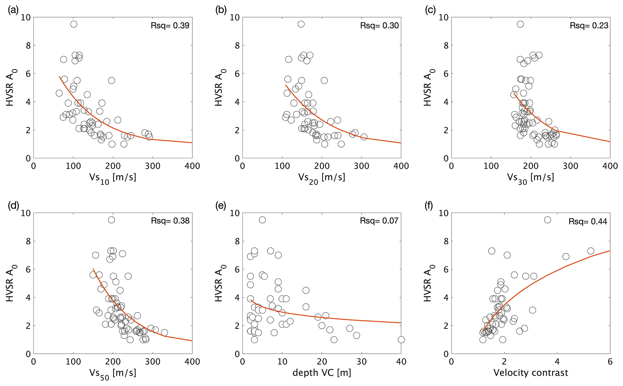
Figure A1 Each panel depicts the fitted function and the coefficient of determination (R_sq) of the HVSR peak amplitude A₀ per G-network borehole location and the corresponding subsurface parameter. The (a) V_s10, (b) V_s20, (c) V_s30, (d) V_s50, (e) depth of the velocity contrast, and (f) size of the velocity contrast.

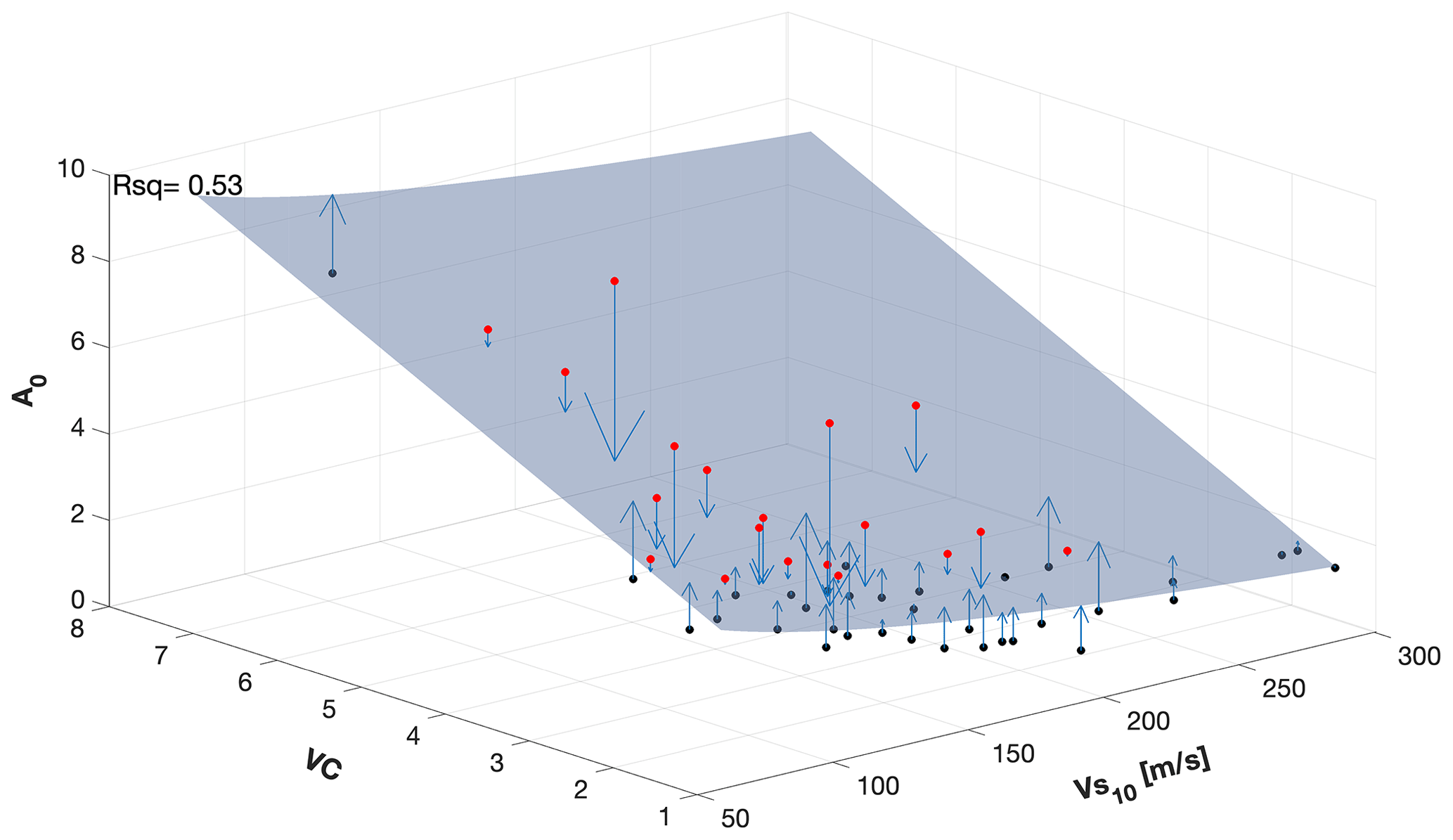
Figure A2 A 3D plot of the two main parameters that define amplification: the velocity contrast and V_s10. The pale blue surface depicts the fitting function between the parameters and divides the data points where the red points are above the surface and black points are below. Blue arrows indicate the difference (error) between the surface and data point.

Compared to individual 1D correlations, a 2D correlation (Fig. A2) using both the VC and the V_s10 results in an improved correlation (R_sq=0.53) and allows us to define an empirical relationship for HVSR peak amplitudes (A₀) based on these two parameters:

$$\begin{array}{}\text{(A1)}& A_{\mathrm{0}}=-\mathrm{1.29}\log \left(\mathrm{0.01}{V}_{\mathrm{s}\mathrm{10}}\right)+\mathrm{0.99}\text{VC}+\mathrm{1.94}.\end{array}$$

Furthermore, this equation supports the hypothesis of Joyner and Boore (1981) and Boore (2003) that A₀ also depends on the VC. The motivation for Eq. (A1) is to achieve an amplification equation based on subsurface parameters only. Using Eq. (A1), an estimate of A₀. is obtained Subsequently, Eq. (1) can be used to obtain an estimate of the amplification factor.

Appendix B: Geological models

B1 GeoTOP

GeoTOP schematises the shallow subsurface of the Netherlands in voxels measuring 100 m by 100 m by 0.5 m (x, y, z) up to a depth of 50 m below ordnance datum (Stafleu et al., 2011, 2021). Each voxel contains estimates of the lithostratigraphic unit the voxel belongs to and the lithologic class (including a sand grain-size class) that is representative for the voxel. GeoTOP is publicly available from the web portal of TNO – Geological Survey of the Netherlands (GDN; https://www.dinoloket.nl/en/subsurface-models, last access: 1 August 2021). GeoTOP is constructed using some 275 000 borehole descriptions from DINO, the national Dutch subsurface database operated by GDN, complemented with some 125 000 borehole logs from Utrecht University in the central Rhine–Meuse river area. The modelling procedure involves four steps: first, the borehole descriptions are interpreted into standardised lithostratigraphic units with uniform sediment characteristics. Given the large number of boreholes, automated lithostratigraphic interpretation routines (Python scripts) were developed. These routines combine digital maps, stratigraphic rules (e.g. superposition), and lithologic criteria (e.g. main lithology, admixtures, grain size, and shell content, amongst other criteria) to determine the depth of the top and base of the lithostratigraphic units in each of the borehole descriptions. Next, 2D interpolation techniques are used to construct surfaces bounding the bases of the lithostratigraphic units as observed in the boreholes. The interpolation algorithm allows for the calculation of a mean depth estimate of each surface and its standard deviation. Subsequently, all surfaces are stacked according to their stratigraphical position, resulting in a consistent layer-based model with estimates of top and base of each lithostratigraphic unit. Top surfaces are derived from the bases of the overlying units. The surfaces are then used to place each voxel in the model within the correct lithostratigraphic unit. In the third step, the borehole descriptions are revisited and classified into six different lithologic classes (“peat”, “clay”, “clayey sand & sandy clay”, “fine sand”, “medium sand”, and “coarse sand and gravel”). In the last modelling step, a 3D stochastic simulation is performed for each lithostratigraphic unit separately. The simulation results in 100 equiprobable realisations of lithologic and grain-size class for each voxel. Post-processing of the realisations results in probabilities of occurrence as well as a “most likely” estimate of lithologic and grain-size class. This most likely estimate is used in the construction of the seismic site-response zonation map (Appendix C).

B2 NL3D

To date, the GeoTOP model covers about 70 % of the country (including inland waters such as the Wadden Sea). For the missing areas we have used the lower-resolution voxel model NL3D, which is available for the entire country (van der Meulen et al., 2013). NL3D models lithology and sand grain-size classes within the geological units of the layer-based subsurface model DGM (Gunnink et al., 2013) in voxels measuring 250 m by 250 m by 1 m (x, y, z) up to a depth of 50 m below ordnance datum. NL3D uses a much simpler modelling procedure than GeoTOP: first, the borehole descriptions are interpreted by intersecting each borehole with the top and base raster layers from the DGM model. The resulting stratigraphical interpretations are geometrically consistent with the DGM model, but not necessarily consistent with the borehole descriptions (e.g. a borehole interval describing “sand” may erroneously fall within a unit that is characterised by clay deposits). Second, the surfaces of the DGM model are used to place each voxel in the model within the correct lithostratigraphic unit. DGM is a layer-based model using a smaller dataset of some 26 500 manually interpreted borehole descriptions from the DINO database. Consequently, it is less refined than GeoTOP. For instance, DGM combines all Holocene formations into a single unit, whereas GeoTOP features some 25 different Holocene formations, members, and beds. The third and fourth steps are identical to the ones described for GeoTOP. The resulting NL3D model has a similar most likely estimate of lithologic and grain-size class which is used in the construction of the seismic site-response zonation map (Appendix C).

B3 Model uncertainty

The current version of GeoTOP covers about 28 605 km² using some 400 000 boreholes. This implies that only about 7 % of the voxels at land surface contain a borehole. Moreover, this number rapidly decreases with depth because many boreholes are quite shallow. Therefore, the lithostratigraphic unit and the lithologic class of almost all voxels are estimated on the basis of nearby borehole descriptions. As a rule of thumb, the limited amount of data available deeper than 30 m below land surface strongly reduces the quality of the lithologic class estimates of GeoTOP (Stafleu et al., 2021). For NL3D, this number is 15 m.

B4 Applicability

GeoTOP and NL3D model the subsurface at a regional to subregional scale that is suitable for applications at the levels of province, municipality, and district. The models are not suited for applications that require a finer scale at the level of streets or individual buildings.

Appendix C: Workflow site-response map

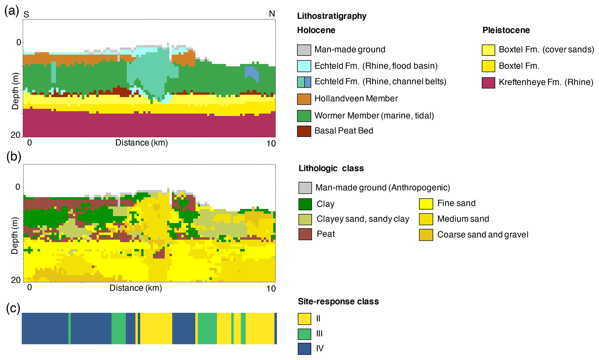
Figure C1 Cross section through the GeoTOP voxel model: (a) lithostratigraphy, (b) lithologic class, and (c) corresponding sediment site-response class. The cross section runs S–N through the city of Alphen aan den Rijn, situated on a sandy Holocene channel belt of the river Oude Rijn (“Old Rhine”). For location see Fig. 13b. Classes III and IV appear where soft, Holocene sediments (clay and peat) are overlying stiff Pleistocene deposits (sand). However, where Holocene sediments are sandy, such as in the channel belt in the centre of the cross section, Class II occurs.

The steps below describe the procedure used to assign the appropriate sediment (site-response) class to each of the voxel stacks in GeoTOP and NL3D, as exemplified in Fig. C1. A voxel stack is the vertical sequence of voxels at a particular (x,y) location in GeoTOP or NL3D. At each voxel there is an estimate of the lithostratigraphic unit and the lithologic class (Appendix B).

• A.1. Calculate the cumulative thickness for each of the lithologic classes (peat, clay, clayey sand & sandy clay, and sand) in the models for multiple depth intervals (5, 10, 20, and 50 m). The thicknesses of the lithologic classes fine sand, medium sand, and coarse sand & gravel have been added together in the superclass sand.

• A.2. Calculate the depth of the top of the first consecutive sequence of sand with a minimum thickness of 1.5 m (GeoTOP) or 2 m (NL3D). This depth is further referred to as “top sand”. In general, “thick” sequences of sand represent the stiffer Pleistocene sediments. In other cases, they may represent Holocene sediments of, for example, the fluvial channel belt systems of the Rhine and Meuse, or the coastal dunes. These sands form the contrast with the overlying soft sediments (peat, clay, and clayey sand and sandy clay). Voxel stacks containing a continuous Pleistocene clay sequence (Elsterian tunnel valleys) are included in the depth of the first sand (top sand), since no amplification is estimated here with the HVSR of site N02.

• A.3. Calculate the percentage of each lithologic class above the top sand. These percentages play an important role in assigning sediment site-response classes as described in steps A.8 and A.9.

• A.4. If anthropogenic deposits reach up to depths larger than 2 m, no sediment class is assigned. Anthropogenic activities have modified the near-surface composition at many locations in the urbanised areas of the Netherlands. The lithologic class of these sediments is unknown. Therefore, we are not able to assign a sediment site-response class to those locations.

• A.5. If bedrock outcrops or occurs at a depth smaller than 2 m, the site is assigned to Class I. The depth criterion is set at a maximum of 2 m since a deeper top bedrock would lead to a top layer with a possible resonance in the 1–10 Hz frequency band and hence a different site-response class. The top of the bedrock is determined from the DGM model (Gunnink et al., 2013) (top surfaces of the Houthem, Maastricht, and Gulpen formations).

• A.6. If bedrock in the eastern and southern parts of the country occurs at a depth of more than 100 m, the sediment site-response class is set to V. These are sites where the layer on top of the bedrock could yield a resonance in the 1–10 Hz band, for which resonance has not sufficiently been calibrated to assign an AF_NL. Class V thus corresponds to sites with a currently unknown amplification potential. The top of the bedrock is determined from the DGM-deep model (Gunnink et al., 2013) (top surfaces of the Rijnland and Chalk groups).

• A.7. If top sand is less than 2 m, the site-response class is set at II. Examples of HVSR curves with top sand less than 2 m do not exhibit any peak amplitude due to the absence of a resonating soft layer on top of a stiffer one.

• A.8. If top sand is between 2 and 3 m, the lithologic distribution of the overlying soft sediments determine if the sediment site-response class will be II, II, or IV. Examples of HVSR curves with top sand between 2 and 3 m show peaks for certain lithological successions, forming a resonating layer. Class II is assigned if the overlying sediments contain more than 60 % sand. Class III is assigned if the overlying sediments are mainly composed of clayey sand & sandy clay and Class IV if clay and peat dominate. We do not elaborate on the exact percentages to decide between Classes III and IV. While testing the different criteria, this step appeared to be quite sensitive and needed the implementation of several exceptions to the general rule.

• A.9. If top sand is larger than 3 m, the approach is basically the same as in A.8. Class II is assigned if the overlying sediments contain more than 60 % sand. However, the exact criteria to decide between Classes III and IV differ from those in A.8.