the Creative Commons Attribution 4.0 License.
the Creative Commons Attribution 4.0 License.
 | 20 Dec 2022
Statistical modelling of air quality impacts from individual forest fires in New South Wales, Australia
Owen F. Price
Wildfires and hazard reduction burns produce smoke that contains pollutants including particulate matter. Particulate matter less than 2.5 µm in diameter (PM2.5) is harmful to human health, potentially causing cardiovascular and respiratory issues that can lead to premature deaths. PM2.5 levels depend on environmental conditions, fire behaviour and smoke dispersal patterns. Fire management agencies need to understand and predict PM2.5 levels associated with a particular fire so that pollution warnings can be sent to communities and/or hazard reduction burns can be timed to avoid the worst conditions for PM2.5 pollution.
We modelled PM2.5, measured at air quality stations in New South Wales (Australia) from ∼ 1400 d when individual fires were burning near air quality stations, as a function of fire and weather variables. Using Visible Infrared Imaging Radiometer Suite (VIIRS) satellite hotspots, we identified days when one fire was burning within 150 km of at least 1 of 48 air quality stations. We extracted ERA5 gridded weather data and daily active fire area estimates from the hotspots for our modelling. We created random forest models for afternoon, night and morning PM2.5 levels to understand drivers of and predict PM2.5.
Fire area and boundary layer height were important predictors across the models, with temperature, wind speed and relative humidity also being important. There was a strong increase in PM2.5 with decreasing distance, with a sharp increase when the fire was within 20 km. The models improve our understanding of the drivers of PM2.5 from individual fires and demonstrate a promising approach to PM2.5 model development. However, although the models predicted well overall, there were several large under-predictions of PM2.5 that mean further model development would be required for the models to be deployed operationally.
- Article
(13991 KB) - Full-text XML
- BibTeX
- EndNote


Smoke from forest fires produces pollutants harmful to human health, which have been linked to tens or hundreds of thousands of deaths per year globally (Chen et al., 2021; Johnston et al., 2012). Particulates smaller than 2.5 µm, i.e. PM2.5 measured as micrograms per cubic metre of air (µg m−3), are of particular concern (Haikerwal et al., 2016; Reid et al., 2016). PM2.5 is a criteria pollutant in regulatory systems for air quality, for example, in the USA National Ambient Air Quality Standards and the Australian National Environment Protection (Ambient Air Quality) Measure.
Hazard reduction burns (HRBs; a.k.a. prescribed or planned burns) and wildfires can both produce high levels of PM2.5. The impact of wildfire-produced PM2.5 on populations, including hospitalisations and premature deaths, varies yearly and spatially depending on wildfire occurrence (Matz et al., 2020; Jaffe et al., 2008), which is driven by droughts, high temperatures and strong winds. Health costs associated with the 2019–2020 wildfires in eastern Australia were estimated to be around AUD 2 billion (Johnston et al., 2021). Massive areas burnt, including over 5×10⁶ ha burnt in the state of New South Wales alone (Filkov et al., 2020), predominantly in eucalypt forests in the mountains and coastal areas between 28 and 38∘ south of the Equator. While wildfire ignitions and sizes are unpredictable, HRBs are controlled fires that are conducted to limit the spread and intensity of future wildfires by reducing fuel amounts. There have been notable instances when HRBs caused poor air quality in large cities (Broome et al., 2016; He et al., 2016; Miller et al., 2019). Large areas of land can be burnt under HRBs; for example, in Western Australia, ∼ 7 % of the forest is treated via HRBs each year (Bradshaw et al., 2018), while in the southeastern USA, millions of hectares are treated each year (Zeng et al., 2008). HRBs also typically occur closer to population centres (Price and Bradstock, 2013) and burn under calm, still weather conditions that may be more conducive to high pollution levels (Di Virgilio et al., 2018). Borchers-Arriagada et al. (2021) found, by comparing population-weighted PM2.5 exposure on days dominated by HRBs or wildfires, that HRBs in New South Wales (NSW), Australia, imposed higher health costs per hectare burnt than wildfires. Further research is required, but differences may stem from different fuel consumption rates (Price et al., 2022), plume behaviour and/or weather.
We need better tools to help understand PM2.5 dispersal and air quality impacts from individual fires. Improving the tools available to forest fire management agencies would improve pollution warnings and indicate changes that could be made to HRB strategies to reduce community PM2.5 exposure, e.g. identifying low-pollution-risk days to conduct HRBs. Attributes of an individual fire that could affect their PM2.5 output and/or exposure of people to PM2.5 are fire size; the rate of heat and smoke production; fire proximity to human populations; and weather conditions including temperature, humidity, wind speed, wind direction, atmospheric stability and differences in weather between the HRB location and the PM2.5 monitor location (Price and Forehead, 2021; Reisen et al., 2015). There is some knowledge about the influence of weather on pollution, but this has been investigated at a larger scale than individual fires. For example, days with HRBs are likely to have poorer air quality in Sydney when there are cool, stable conditions with light westerly winds (Di Virgilio et al., 2018), while poor air quality, as measured by ozone levels, tends to occur with a high-pressure system to the east of Sydney with light north-westerly winds and a sea breeze (Hart et al., 2006).
There are a variety of ways to improve our understanding of PM2.5 from individual fires. Atmospheric dispersion models can predict the spread of particulates from fires based on modelled atmospheric dynamics and are routinely used in many countries to guide burning operations and community warnings for HRBs. However, while evaluations of such systems are rare, existing evaluations indicate a poor to moderate agreement between predictions and observations (Yao et al., 2014; Saide et al., 2015), possibly because the local effects of HRBs are poorly captured by the models.
An alternative method is to relate air quality observations directly to real fires to calculate how far the smoke impact is likely to spread and under what conditions. Air quality measurements can be from ground-based stations or via satellite-based measurements, e.g. aerosol optical thickness (Gupta et al., 2007). For ground-based measurements, studies have been carried out using monitors mostly stationed within ∼ 10 km of HRBs (Pearce et al., 2012; Price and Forehead, 2021). Pearce et al. (2012) made 684 observations of daily mean PM2.5 by placing monitors around 55 HRBs. They found that PM2.5 concentrations fell to near-background levels within 3 km of the fire perimeters. Price and Forehead (2021) made 5445 hourly observations of PM2.5 with a combination of fixed and mobile monitors around 18 forest HRBs. They also found that PM2.5 concentrations had largely fallen to background levels by 3 km, but this depended on weather conditions. One of the HRBs caused poor air quality at monitors more than 30 km away. These studies captured the local effects of the HRBs but did not explain why HRBs can impact air quality much further away.
Deploying air quality monitors to wildfires is difficult due to the large size of wildfires, unpredictable ignition and spread, and the safety risks of working near an active wildfire. However, large permanent air quality monitoring systems can be used to gather PM2.5 data for wildfires and HRBs, for example, the NSW air quality monitoring network. Here, we used historical fire and air quality data to identify the occasions when an individual fire was burning within 150 km of a monitor in the NSW air quality monitoring network from 2012 to 2021, and we developed random forest models of PM2.5 concentrations at individual monitors as a function of fire area, distance and weather conditions. Our aims were
-
to improve understanding of the fire and weather conditions that influence smoke dispersal and PM2.5 levels;
-
to develop predictive models of PM2.5 output from individual forest fires, as a complement to physical models, to improve warnings; and
-
to make inferences about potential changes in HRB protocols that could reduce PM2.5 impacts.
2.1 Fire data
Our study period was from February 2012 to September 2021 because this was when our main fire dataset was available (see below). For the study period, we created a spatial dataset of forest fires that were actively burning within 150 km of air quality monitoring stations (AQSs) maintained by the NSW Department of Planning and Environment (DPE) (Fig. 1). The 150 km criterion captures most of the eucalypt-dominated Blue Mountains that are subject to the majority of fire activity near Sydney. We assigned attributes of fire location, fire type (hazard reduction burn (HRB) or wildfire (WF)), date of fire activity, and AQS name and location. Each fire had at least one active date, and most burnt on several days. As a fire could be within a 150 km buffer of multiple AQSs, there was a separate row in our data for each fire and AQS combination. For our modelling, we used only cases where, for each AQS and day, only one fire was active within 150 km of the AQS. We did not analyse cases where multiple fires were burning on the same day near the same AQS as it was unclear which fire produced the smoke that reached the AQS.
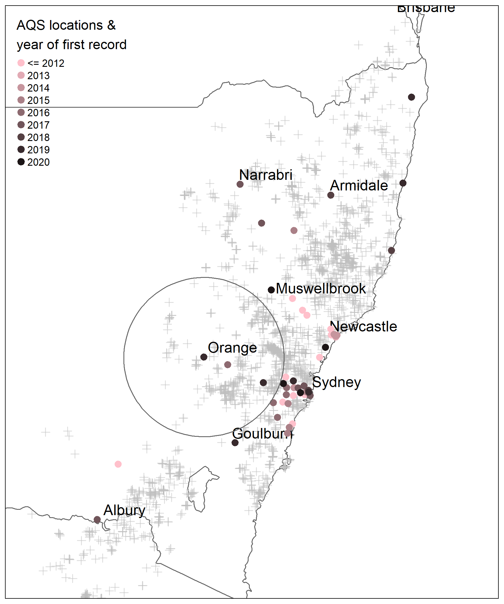
Figure 1Map of the study area (New South Wales, Australia) showing air quality monitoring stations (AQSs, n = 48), coloured by year of first PM2.5 record. Grey crosses are the locations of all fires used in analysis, with one cross per fire per day. The 150 km buffer is shown around Orange AQS as an example (all AQSs had 150 km buffers for analysis).
We relied on two data sources to identify fire locations, type and active dates: NSW fire history GIS polygons (NPWS Fire History – Wildfires and Prescribed Burns, 2022), maintained by the NSW National Parks and Wildlife Service (NPWS), and Visible Infrared Imaging Radiometer Suite (VIIRS) – Suomi National Polar-orbiting Partnership (SNPP) hotspots, downloaded from NASA's Fire Information for Resource Management System (FIRMS; Schroeder et al., 2014). VIIRS SNPP hotspots were available beginning 20 January 2012.
The fire history dataset is a spatial polygon dataset of the final burnt area of fires across NSW and has attributes of fire identity (name and number), fire type (HRB or WF), and start and end dates. We did not rely solely on the fire history to identify fire locations and dates because an initial inspection suggested some issues for our analysis. These included fires identifiable from VIIRS hotspots that were missing from the fire history; occasional errors in the start and end date recording; the final fire polygon being the combination of separate fires that eventually merged; and the data identifying only fire start and end date, not whether a fire was actively burning on each day between those dates (e.g. fires may have been extinguished then reignited on different days). Also, the data captured only the final fire boundary and not daily fire progression, meaning the location of fire activity on the first day (perhaps a few hectares) was not well represented by the final fire polygon (perhaps tens or hundreds of thousands of hectares), which was particularly an issue for WF.
We employed a process to identify active fire dates and locations from clusters of VIIRS SNPP hotspots. We used VIIRS SNPP hotspots instead of MODIS as VIIRS has higher resolution (at nadir, 375 m vs. 1 km for MODIS) and thus can detect more hotspots per fire than MODIS, which reduces the chance that an active fire is missed (Schroeder et al., 2014). The process to create hotspot clusters for each day for each AQS was as follows:
-
Extract all hotspots within 150 km of the AQS. Hotspots for one “day” in our analysis included those acquired in the early afternoon (day hotspots) and over the following night (night hotspots).
-
Focus on forest fires, and remove hotspots that were in grassland or open woodland by removing hotspots with a low foliage projective cover score (Gill, 2012; Gill et al., 2017). This measure of canopy density is equal to the proportion of ground that the vertically projected area of the green foliage covers. We removed hotspots with a cover fraction of less than 0.25 so that our analysis only included dense woodlands, open forests and closed forest types (Specht and Specht, 1999).
-
Buffer each hotspot by 2.5 km, and dissolve overlapping buffers into a single polygon, thus creating hotspot cluster polygons (Fig. 2).
-
Remove clusters that did not have at least five day or night hotspots. This was our minimum threshold for fire activity, as we wanted to exclude small fires such as burning heaps on farmland that can be detected by VIIRS. We also tested three as a minimum threshold, which produced similar but slightly less accurate models.
-
For each cluster, calculate the daily active fire area by intersecting the hotspot points with a 500 m × 500 m grid (25 ha cells). The area assigned to each cluster was the number of unique intersecting cells × 25 ha.
-
Repeat the process for each combination of date and AQS.
Where a fire identified from the above process (a “VIIRS fire”) intersected an NPWS fire history polygon between its start and end date, we assigned the fire name, number and type (HRB or WF) to the VIIRS fire. If multiple VIIRS fires intersected the same fire history polygon, we merged them into a single fire with the same attributes for analysis. If a VIIRS fire intersected multiple fire history polygons, we assigned the attributes from the fire history polygon with the largest overlapping area. NPWS fire history polygons were excluded from analysis either if the start or end date was missing or if a polygon had no intersecting VIIRS hotspots. If a VIIRS fire did not intersect a fire history polygon, we assigned the fire type based on the date: from October to February (inclusive) was WF, and all other months were HRB. For each fire identified we added attributes of distance and direction from AQSs to fire centroids (Fig. 2), i.e. the arithmetic mean of the hotspot coordinates, with a separate row for each fire and AQS combination (within 150 km).

Figure 2Example of creating clusters from VIIRS SNPP hotspots. Black dots are hotspots; red asterisks are fire centroids, i.e. the arithmetic mean of the hotspot coordinates. The image has two separate fires. Each hotspot is buffered by 2.5 km, with all overlapping buffers merged and hotspots given separate identity numbers based on which final buffer they fell within. Two separate fires are created here because of distinct fires where buffers do not overlap, i.e. greater than two buffer widths (5 km) apart. Fire 1 (grey) has > 50 hotspots; fire 2 (blue) has 5 hotspots. Note that the fire area used in analysis was calculated via an intersection of hotspots with a 500 m × 500 m grid and not via buffer size (see Methods).
2.2 PM2.5 data
We modelled PM2.5 (µg m−3) as a function of several environmental predictors. We downloaded all available PM2.5 data (hourly averages) from the NSW DPE for the period 2012–2021, which comprised 48 AQSs. Data were available free online at https://data.airquality.nsw.gov.au/docs/index.html (last access: 1 June 2022). We calculated mean PM2.5 for each AQS for three 6 h periods:
-
Afternoon, 14:00 to 19:00 AEST inclusive. This period covered peak burning conditions in the afternoon and after sunset, although sunset and fire ignition times varied.
-
Night, 21:00 to 02:00 AEST inclusive. This covered the night period starting on the same day as the fire.
-
Morning, 05:00 to 10:00 AEST inclusive, next day after fire day. This captured conditions early the next morning after the main periods of fire activity were likely to have ended, although some fires may have burnt through the night and smoke may still have lingered.
Note that there were some missing PM2.5 values in the data, which meant some summary afternoon/night/morning values had < six records. However, > 98 % of records were summarised from ≧ four hourly PM2.5 values.
We chose these times to represent different periods in the daily cycle that may have distinct smoke, weather and fire behaviour characteristics. All fires identified in the hotspot analysis were matched to AQS summary PM2.5 for active days when the fire was within 150 km. Not all AQSs had records for all years, as some were not operational until later in the study period (Fig. 1). Note that we modelled PM2.5 observed at air quality stations, which included primary and secondary PM2.5. Secondary PM2.5 can be formed via atmospheric chemistry processes that transform emitted gases into particulates, with the processes influenced by factors including season, solar radiation, temperature and relative humidity (Cope et al., 2014; Fine et al., 2008).
2.3 Predictor variables
We sampled hourly weather variables at each AQS and each fire centroid from ERA5 weather grids, which constitute an atmospheric reanalysis product with multiple weather variables and atmospheric levels available at 30 km spatial and hourly temporal resolution (Hersbach et al., 2018b, a) (Table 1). We calculated the mean weather values for both surface and upper atmospheric conditions (Table 1) for the afternoon, night and morning periods as described for PM2.5. We calculated additional variables describing the spatial relationship between the fire and each AQS. We used the AQS-to-fire direction and wind direction to calculate the percent of time period when the surface wind was blowing directly to the AQS, with directly meaning ±22.5∘ of the AQS-to-fire bearing. We also used the daily active fire area based on the intersection of hotspots and a 500 m by 500 m grid (area = N intersecting cells × 25 ha) as a predictor. We included a month variable (i.e. month of the active fire date) as a predictor variable to account for any seasonal variation in background PM2.5 levels. The month was represented as a cyclic variable, where the sine and cosine of the month (1–12) were both included in the modelling. We included the latitude and longitude of the AQS to account for spatial dependence, and we included fire type as a factor variable to account for differences not captured by the weather or fire area variables. We also experimented with making separate models for each fire type (HRB model and WF model) for each time period but found that resulting accuracy statistics on the training and test sets were similar, so instead we just used one model for each time period with fire type as a factor variable.
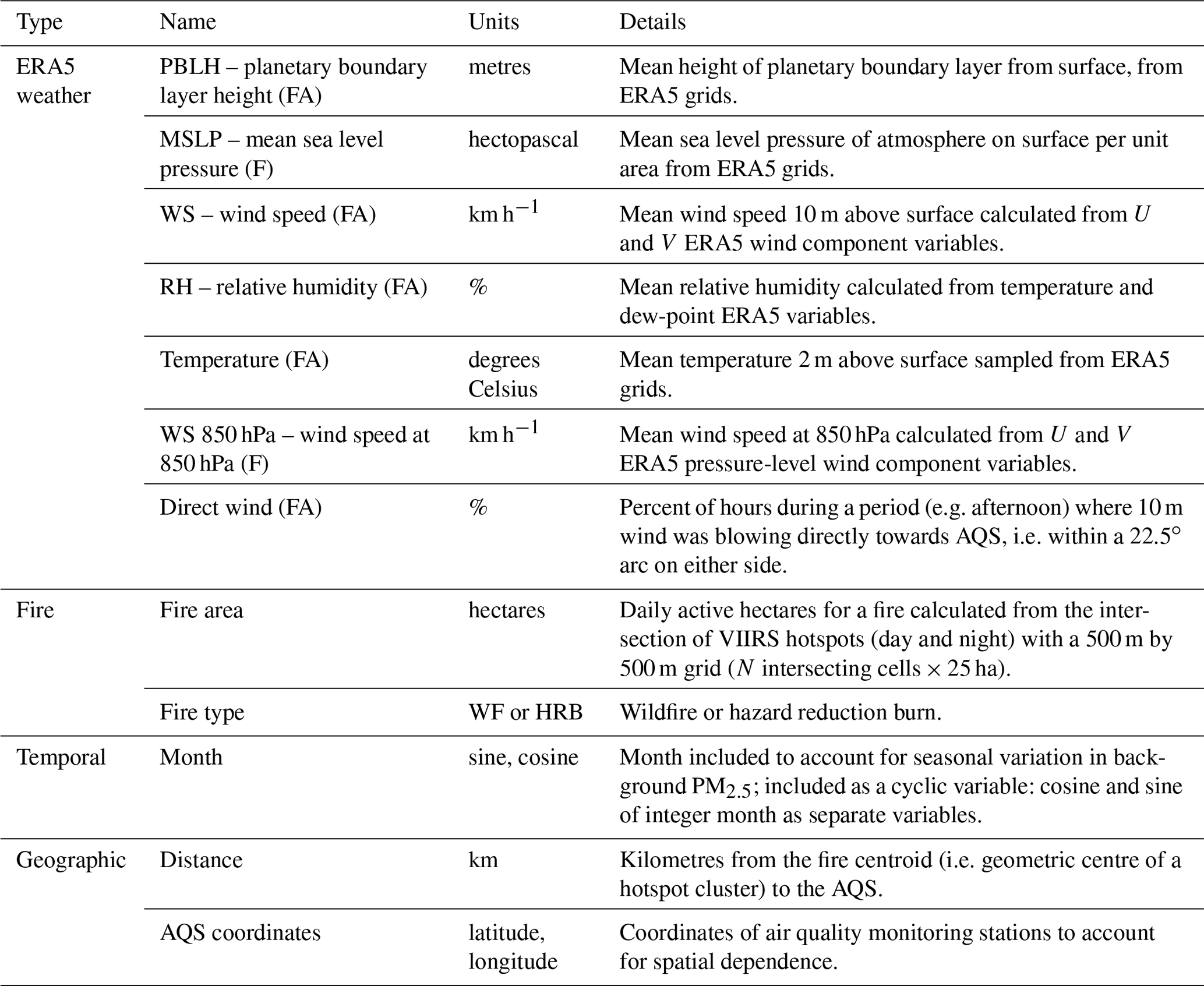
Table 1Predictor variables used for random forest modelling. Letters mean that for the random forest modelling weather variables were sampled at the fire (F), at the AQS (A) or both (FA). MSLP and wind speed (850 hPa) at the AQS were excluded due to being highly correlated with the same variable at the fire.
2.4 Random forest modelling
Our data consisted of three separate tables (afternoon, night and morning data tables) for three models. In each table, there were 11 187 rows with unique combinations of fire, AQS and date. For each fire, there could be multiple active dates, and each fire could be associated with more than one AQS (i.e. it was within 150 km of multiple AQSs). Our data had 48 different AQSs and 1429 different days with at least one active fire near an AQS. There were 1883 different combinations of fire and day (we refer to these combinations as “fire–days”) consisting of 727 fire–days that had VIIRS hotspots and a fire history record and 1156 fire–days that had only VIIRS hotspots. The fire–days from solely VIIRS hotspots were on average smaller than the fire–days with a matching NPWS fire history record (209 ha vs. 854 ha respectively). A total of 1182 fire–days were from HRBs (mean daily active fire area = 254 ha), and 701 were from WFs (mean daily active fire area = 802 ha). Each fire was observed at a minimum of 1 AQS, with a mean of 6 AQSs and a maximum of 35 AQSs associated with a single fire.
We trained a random forest model using the “ranger” package in R (Wright and Ziegler, 2017). Random forests are robust and efficient machine learning algorithms that involve fitting and averaging of randomised decision trees and have been applied to a range of environmental research problems including fire and emissions (Biau and Scornet, 2016; Hu et al., 2017; Shah et al., 2022). We chose random forests due to several advantages that include high accuracy, fast computation times, easy implementation, robustness and greater interpretability (compared to “black-box” methods) via simple methods to extract variable importance and partial dependence (Rodriguez-Galiano et al., 2015; Biau and Scornet, 2016; Wright and Ziegler, 2017).
We split each of our datasets into training (75 %) and test (25 %) sets for analysis, stratified by fire type so that an even proportion of HRBs and WFs appeared within each of the sets. We trained the models using the training set data and used out-of-bag (OOB) predictions vs. observations for model accuracy checks, and we predicted on the test set to calculate test set accuracy statistics. Our accuracy statistics were the correlation coefficient (r), normalised mean error (NME) and normalised mean bias (NMB), as recommended by Emery et al. (2017) for assessing model performance. We ran three different models, one for each analysis period: (1) afternoon mean PM2.5, (2) night mean PM2.5 and (3) morning mean PM2.5. Predictor variables were the weather variables in Table 1 sampled at both the AQS centroid and the fire centroid, distance, daily active fire area, month, and AQS coordinates. As highly correlated variables can introduce bias into random forest variable importance calculations (Strobl et al., 2008), we removed variables from analysis where the Pearson correlation was above 0.8: mean sea level pressure (MSLP) at AQSs and wind speed at 850 hPa at AQSs were excluded, each of which was correlated with the version sampled at the fire.
We assessed the variable “permutation” importance using the ranger package. Permutation importance is derived from a process where reduction in model accuracy for OOB predictions is calculated after randomly shuffling values for each variable, calculated for all trees and variables (Wright et al., 2016). We assessed predictor variable effects using partial dependence plots calculated in the “pdp” package in R (Greenwell, 2017) and by creating prediction plots where PM2.5 was predicted with all variables held at mean values except two variables of interest, which were each assigned three different levels to illustrate their effects. We also conducted a short descriptive analysis, using satellite images and hourly PM2.5 of large outliers in the models to understand potential reasons for inaccurate predictions. This is included in Appendix A.
2.5 Limitations
There are several limitations to our methods that should be considered when interpreting the results. Our process to identify active fires from VIIRS hotspots excluded hotspots that were outside the 150 km AQS buffer, even if they were part of a fire that straddled the buffer edge. There may be occasions where smoke from hotspots, as well as entire fires, from > 150 km reached an AQS and influenced PM2.5, e.g. large WFs during the 2019–2020 “Black Summer”. The effect of such fires was not captured in our methods.
We set a minimum fire activity threshold of five hotspots (day or night). This may mean that days recorded as having only one fire may have had other smaller fires in the area that may have produced smoke that affected PM2.5. Relying on VIIRS had the advantage of being able to better detect when a fire was active, but our process may not have captured all fires on any given day due to cloud cover impeding VIIRS hotspot detection. This may be a form of bias in our analysis as the cloudiest days were selected against. Additionally, VIIRS SNPP hotspots are acquired in the early afternoon and early morning, meaning that only the active area at the time of VIIRS acquisitions is measured and not the total burnt area over a day. Fire area or the number of fires may have been underestimated if clouds were impeding hotspot detection. Our decision to analyse only days with one fire, to better understand distance and direction variables, means that there is a selection bias against the most active fire days (i.e. days with multiple fires). This may include the worst WF days, where multiple fires were more likely to ignite, particularly during 2019–2020. For days that are most suitable for HRBs, authorities are more likely to ignite multiple HRBs. Such days, which could include the worst pollution events, were not included in our analysis but have been the subject of separate research (Storey and Price, 2022).
Note that in our VIIRS hotspots clustering process, we used a buffer of 2.5 km to provide a broad “search” area in which to group hotspots: any hotspots within 5 km of each other (two buffer widths) or less would be grouped. This may have meant that on some occasions, separate small fires were grouped. However, we deemed it reasonable to treat these as one fire for our purposes given that the similar location meant smoke would be travelling along the same general bearing towards an AQS, which was important for the direct wind variable (Table 1). For example, two fires 5 km apart would have a ∼ 3∘ difference in bearing to an AQS 100 km away (∼ 5∘ at 50 km). Smaller or larger buffers may have produced different results. Note that if more than one hotspot cluster intersected the same NPWS fire history polygon, we also treated these as the same fire.
3.1 Variable summaries
Plots of the distribution of PM2.5 and predictor variables are shown in Fig. 3. PM2.5 was skewed towards low values (afternoon, night, morning mean = 8.1, 10.7, 10 µg m−3), with occasional very smoky periods (afternoon, night, morning maximum = 294.2, 394.8, 506.2 µg m−3). Most fires were between 75 and 150 km from AQS, and only 20 % of fires had their closest AQS within 50 km. The daily active fire area derived from VIIRS hotspots was heavily skewed towards lower values (mean = 458 ha, 95th centile = 1175 ha). The maximum fire area was 31 800 ha; < 1 % of fires (all WF) were over 10 000 ha and 94 % were less than 1000 ha.
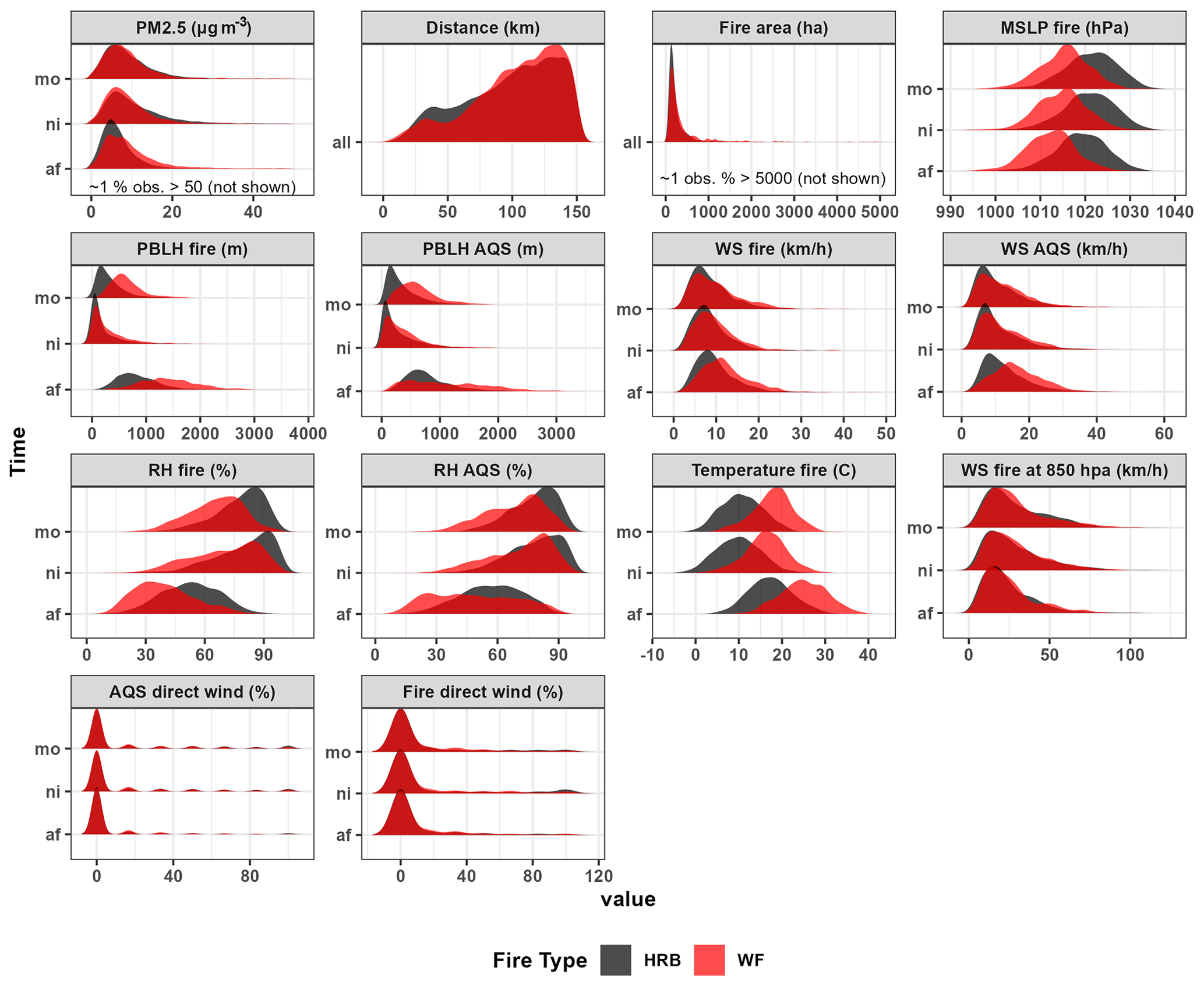
Figure 3Distribution of PM2.5 and predictor variables used in random forest modelling, excluding latitude, longitude, fire type and month. Distance and daily active fire area are daily variables, so they are identical for afternoon, night and morning model datasets. Distributions for at-fire variables are from unique fire–day combinations, at-AQS variable values are from unique AQS-day combinations. af, afternoon; ni, night; mo, morning; AQS, air quality station; RH, relative humidity; WS, wind speed; PBLH, planetary boundary layer height; MSLP, mean sea level pressure.
Afternoon conditions were generally hotter, were less humid and had higher PBLH at both fire and AQS locations than in night and morning conditions. Between WF and HRB, WF afternoons were hotter, were drier and had higher PBLH (Fig. 3). MSLP was similar between afternoon, night and morning but skewed lower for WF compared to HRB. The wind direction variables were clustered around zero, indicating that most of the time wind at the fire and at the AQS was not moving smoke directly from the fire to the AQS (Fig. 3). For example, only 5 % of rows in the afternoon data indicated that wind sampled at the AQS was coming directly from the fire for at least 3 of the 6 h. For wind sampled at the fire, this figure was 11 %.
3.2 Highest-PM2.5 days
Figure 4 shows the 20 highest mean PM2.5 values for each 6 h period for HRBs and WFs. The top PM2.5 values were much greater for WFs than for HRBs in the afternoon, night and morning (∼ 150 to 200 µg m−3 greater for each). Of the top 20 PM2.5 values for WF for afternoon, morning and night, ≧ 80 % were associated with the 2019–2020 wildfires in NSW, many with the Gospers Mountain wildfire in the Blue Mountains (Boer et al., 2020).
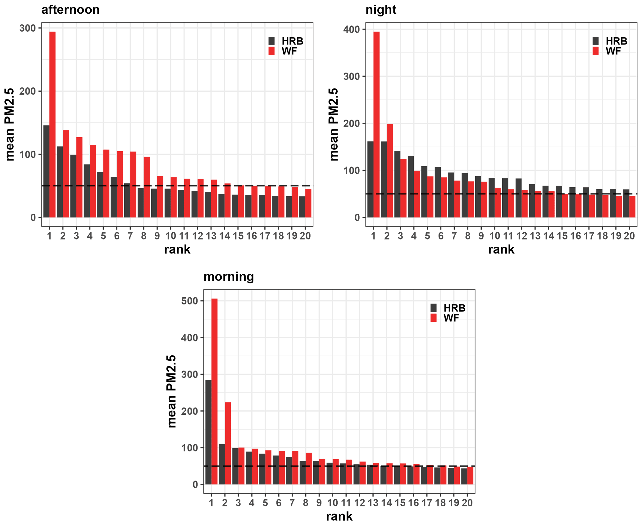
Figure 4Highest mean PM2.5 values for each 6 h time period for HRBs and WFs. For each date, only the single top value from all AQS values is shown (i.e. the second highest for each date is not shown). The dashed line indicates 50 µg m−3 for reference between the three plots. Note that our data only include situations with one fire within 150 km of an AQS for a particular date.
The top seven afternoon peaks for WF were > 100 µg m−3 (max = 294 µg m−3), but only two of the afternoon HRB peaks were > 100 µg m−3. In the night and morning, there were fewer values > 100 µg m−3, but larger maximums were recorded for HRB and WF for each period (compared to the afternoon). For each rank position, WF values were greater than HRB values, except in the night model where, from positions 3 to 20, the HRB values were higher. More information on the conditions surrounding the worst PM2.5 events for each time period for HRBs and WFs, including satellite images, weather plots and descriptions, is included in Appendix A.
3.3 Model results
Daily active fire area, PBLH (fire and AQS), temperature and RH at the fire were among the most important variables in the three models (Fig. 5). Some variables were among the most important in only one or two of the models: wind speed at the fire was the fourth and fifth most important in the night and afternoon models but ninth most important in the morning model. The direct wind variables, distance to fire, AQS coordinates, MSLP, month and fire type were all of moderate to lower permutation importance in each model.
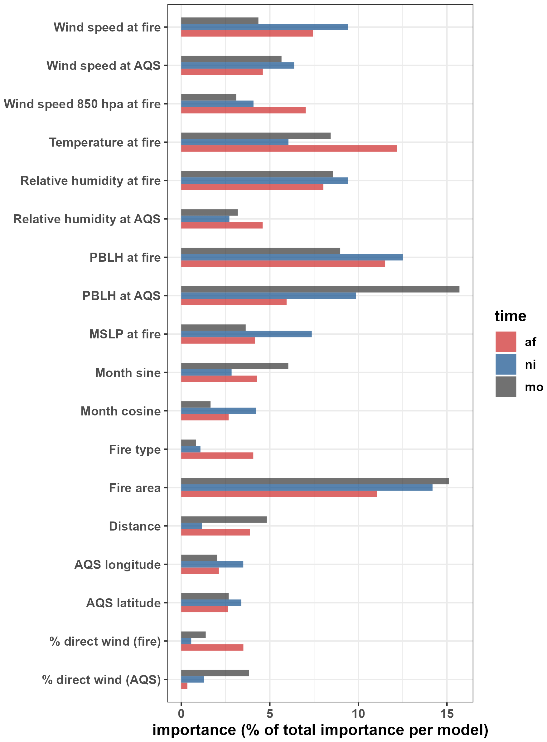
Figure 5Variable importance for each model. A common x scale was assigned, which is the percentage of the total permutation importance attributable to each variable (i.e. importance sum (importance) × 100).
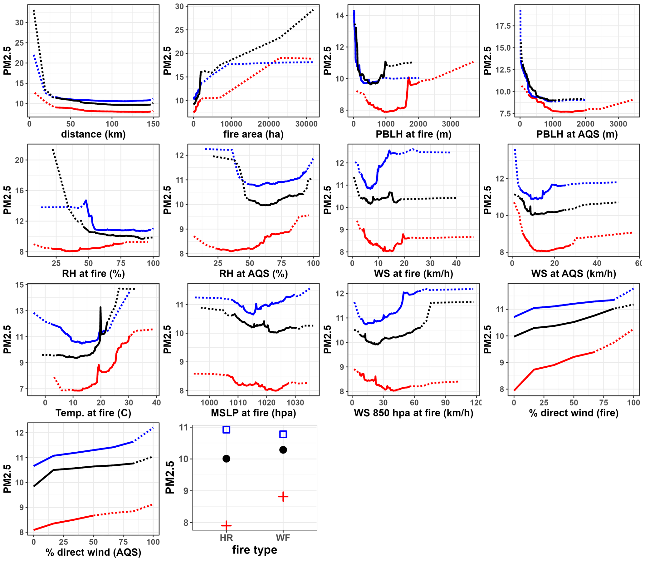
Figure 6Partial dependence plots for the afternoon (red), night (blue) and morning (black) models. Dotted parts of lines are minimum to the 5th centile and 95th centile to maximum values for each predictor variable, calculated from the training data. Where dotted parts are long, this indicates a large range of values with a small number of observed points for model training.
Partial dependence plots (Fig. 6) indicated that for all models, there was a sharp increase in predicted PM2.5 when the AQS-to-fire distance was below ∼ 20 km, with the morning model displaying the sharpest rise in PM2.5 as the distance decreased. This effect is despite distance being of middle to lower permutation importance (Fig. 5). Partial plots indicated PM2.5 increased as fire area increased, particularly in the 0–2500 ha range, which is where most training observations were situated (Fig. 3). There was a very large PM2.5 increase above 10 000 ha in the morning and afternoon models, although there is uncertainty here due to a small number of training observations > 10 000 ha (Fig. 3). The shape of the PBLH effect differed for each model between the fire PBLH and AQS PBLH. At the AQS, there was a strong negative effect of PBLH (lower PBLH means a higher PM2.5), particularly in the night and morning models < 500 m. At the fire, each model had peak PM2.5 at low and high values of PBLH. For the night and morning models, PM2.5 peaked when fire PBLH was ≲200 m, with a smaller rise ≳800 m. For the afternoon model, the largest peak was when fire PBLH was high (≳ 1500 m), with a smaller rise when ≲ 500 m. For RH at the fire, predicted PM2.5 below ∼ 50 % RH was much higher than when RH was above 50 % in the morning and night models. For wind speed, effects varied between the fire and AQS and with the time period: lower wind speed at the AQS was associated with higher PM2.5 in all models but at the fire low and high (particularly for the night model) wind speeds were associated with higher PM2.5.

Figure 7Predictions of each model on the test set, with points coloured by fire type. The Pearson correlation of predictions to observations by fire type is shown in text (r).
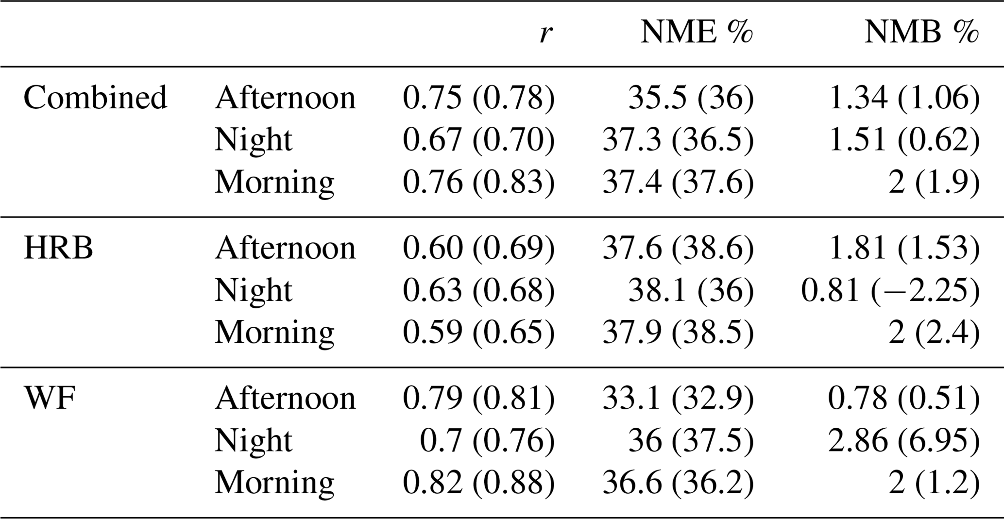
We calculated model accuracy statistics for the training set (OOB predictions) and the independent test sets and for HRB and WF subsets of each. From the combined statistics, Pearson correlations between predictions and observations (r) for training and test sets ranged from 0.67 to 0.83 (Table 2, Fig. 7). For the statistics by fire type, r was higher for WF than for HRB. For WF, r was 0.7 to 0.88 on the training and test sets. For HRBs, r was 0.59 to 0.69 on the training and test sets. NME for all combinations of training/test set and fire type ranged between 33 % and 39 %, with the lowest NME for the WF subset from the afternoon model (∼ 33 % for training and test set). The normalised mean bias (NMB) indicated that generally there was a slight over-prediction bias that ranged from ∼ 1 % to ∼ 2 %, with a maximum of 6.95 % for WF for the night model test set. The night model had under-prediction bias for HRBs on the test set (Table 2, Fig. 7).
Table 2Accuracy statistics from random forest modelling for training and test (in brackets) sets. Training set predictions are on out-of-bag samples during model fitting, and test set predictions were made on the independent test set. Overall statistics, along with statistics on HRB and WF portions of the data, are shown. r, Pearson correlation; NME, normalised mean error; NMB, normalised mean bias (Emery et al., 2017).
The models had large under-predictions for the largest PM2.5 values and a few large over-predictions (Fig. 7). NMB calculated on data that included only where observed PM2.5 was ≧ 20 µg m−3 was −30.9 % (training) and −32.8 % (test) in the afternoon model, −34.5 % and −35.8 % in the night model, and −29.6 % and −32.3 % in the morning model, indicating under-prediction bias for the larger PM2.5 values. For predictions on the test set, in the afternoon model nine observations were under-predicted by at least 30 µg m−3, four from WF and five from HRB. The maximum over-prediction was by 36 µg m−3. For the night model, there were 15 occasions where the model under-predicted in the test set by at least 30 µg m−3 (12 were HRB). The maximum over-prediction was by 57 µg m−3. The morning model had 14 under-predictions on the test set by at least 30 µg m−3, with the largest under-prediction by 175 µg m−3 for a 2019–2020 WF, although the model correctly predicted this morning as having the highest PM2.5 in the test set (observed: 390 µg m−3, predicted: 215 µg m−3). There were three over-predictions by at least 30 µg m−3.
We explored the influence of distance and some selected variables with a series of prediction plots (Fig. 8). PM2.5 was predicted to increase substantially with decreasing distance within the first 20 km of the fire in all combinations of area, PBLH, RH and temperature. Beyond ∼ 30 km there was a minimal effect to no effect of distance, except in the morning model with a large fire area (Fig. 8a). The effect of temperature at the fire differed between models, such that as temperature increased from 10 to 25 ∘C, PM2.5 was predicted to decrease in the morning model but increase in the afternoon model. The plots also suggest there is generally a small difference between predicted mean PM2.5 for WF and HRB for each model once the other predictors including fire area are controlled for.
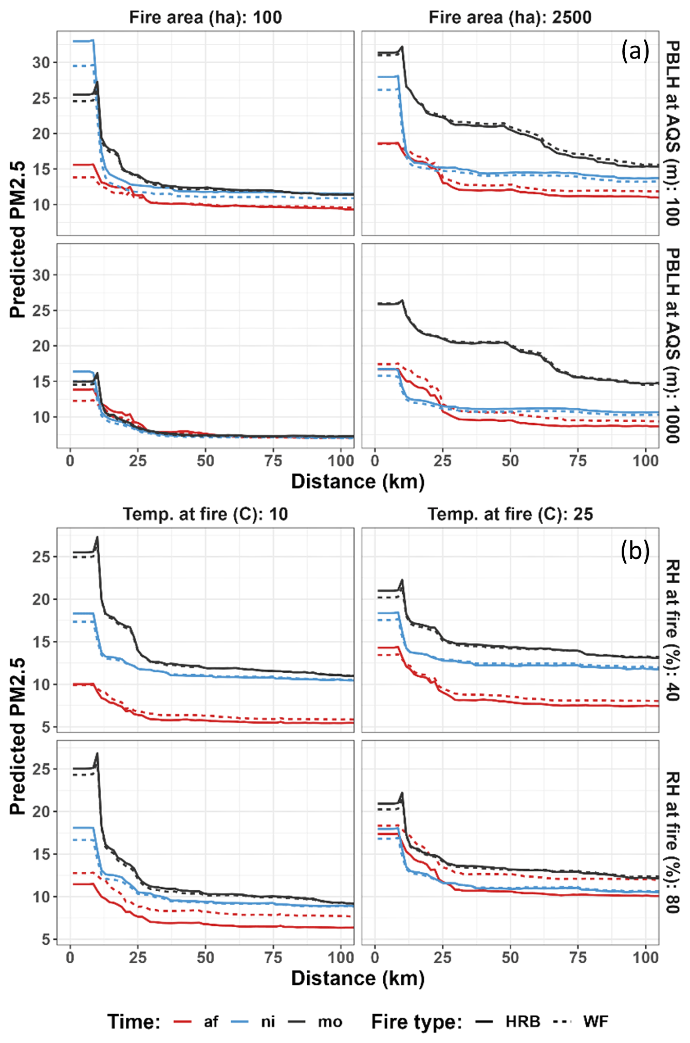
Figure 8Predicted effects of selected variables on mean PM2.5. Colours are time periods; line types are fire types; grid squares are combinations of the daily active fire area and planetary boundary layer height at the air quality monitoring station (a) and relative humidity and temperature at the fire (b).
Using empirical fire and air quality monitoring station data, we identified important drivers of particulate pollution associated with individual forest fires. The results are important in the context of our first research aim, which was to improve understanding of the fire and weather conditions that influence smoke dispersal and PM2.5 levels. In our models, daily active fire area, PBLH, temperature, relative humidity and wind speed were all important drivers of PM2.5 from individual fires. The importance of these variables at the fire or at the AQS varied between models. Distance to fire generally had low permutation importance, possibly due to the low number of AQSs in the 0 to 50 km range (Figs. 3, 6). However, partial plots and prediction plots indicated a large influence on model predictions. For example, partial and prediction plots suggested that within 20 km of a fire, PM2.5 levels rose steeply with decreasing distance. The effect of distance > 50 km was negligible in most cases, suggesting other factors are more important drivers at such distances, although under certain conditions there could be raised PM2.5 at long distances, such as with larger fire area in the morning model (Fig. 8). Based on Reisen et al. (2018), a 1000 ha prescribed burn will emit 160 t of PM2.5, enough to fill to exceedance level a cylinder capped by a planetary boundary layer of 500 m to a radius of 64 km. This means there are sufficient particulates available for a distance effect to occur should the weather conditions suit. Other authors have found similar variables to be important in modelling PM2.5, including fire size and distance when PM2.5 was measured within ∼ 10 km of HRBs (Pearce et al., 2012; Price and Forehead, 2021). PBLH was also a consistent predictor of PM2.5 levels at multiple stations in Sydney during HRB days (Di Virgilio et al., 2018). However, studies such as these have modelled PM2.5 over smaller scales than we did here or did not attempt to link individual fires to PM2.5 records. Our data included PM2.5 measurements up to 150 km from a fire, and we built PM2.5 models using a much larger dataset of fires and PM2.5 records, which here were from pre-installed permanent AQSs. Therefore, the results from our study are more applicable to the individual fire-and-PM2.5 relationship across large geographical areas than other studies.
Our models suggest the area potentially affected by PM2.5 from fires is larger than in Price and Forehead (2021), where raised PM2.5 levels were mostly modelled to be within 5 km of HRBs. Here, our models suggested that raised PM2.5 levels mostly occurred within 20 km of a fire. Our dataset includes a larger set of fires and includes WFs, which are likely to produce smoke that travels further. In some individual cases in our raw data, fires caused high PM2.5 levels > 100 km away (e.g. Appendix A, Fig. A3). Although relatively sparse, analysis using the more remote AQS network is more suited to detecting these longer-range effects than when monitors are placed only close to a fire.
Our second aim was to develop predictive models of PM2.5 output from individual forest fires, as a complement to physical models, to improve warnings. There was some success here: r on the test sets indicated moderate to good agreement between predictions and observations: 0.78, 0.70 and 0.83 for the afternoon, night and morning models respectively. The models fit better on the WF portion of the test data (r 0.76 to 0.88) than for HRBs (r 0.65 to 0.69). The better results for WF suggest the models may be more applicable to WFs, e.g. for the issuance of pollution warnings due to WF smoke. An important consideration for using the models for prediction is their accuracy on the highest PM2.5 observations. Events with very high PM2.5 have the largest health impacts and are therefore the most important to predict, for example, to correctly issue warnings or defer HRBs due to high pollution risk. Our results suggest that, while some predictions for the highest PM2.5 observations were relatively accurate, the models did not consistently predict larger PM2.5 events, so they may not be suitable as an operational prediction tool without further development.
There are several possible reasons for the biggest outliers and limited accuracy. The AQS network is relatively sparse, being concentrated in Greater Sydney, making the distance between any fire and AQS usually large. The mean distance to the closest AQS for each fire–day was 88 km (10th centile = 31 km). This may partly explain why we did not detect wind direction effects. Price et al. (2012) also did not find significant effects of wind direction when modelling PM2.5 in relation to MODIS hotspots at similarly broad scales around Sydney and Perth. In contrast, two empirical studies that did detect clear wind direction effects from HRBs, Pearce et al. (2012) and Price and Forehead (2021), placed PM2.5 monitors close to HRBs, mostly within ∼ 10 km. The large distances in our data mean smoke was subject to broader weather circulation patterns before reaching an AQS, such as shown in Appendix A. This could create a varying lagged pollution effect that we did not completely account for in our modelling because smoke may take different amounts of time to reach an AQS depending on circulation patterns. Although we did not focus exclusively on coastal areas, many AQSs were in coastal areas, so they may have been affected by complex wind patterns. The Sydney basin, for example, can be affected by westerly terrain-related drainage flows, sea breezes and their interaction (Jiang et al., 2017). Differences between land and sea temperatures can influence local wind patterns in coastal areas, creating situations where pollutants emitted overnight or in the morning and blown out to sea are recirculated back over (or near) the source area with a developing sea breeze (Yimin and Lyons, 2003; Levy et al., 2008). Such effects were not accounted for in our study but have been the focus of other research that has used recirculation metrics (Di Bernardino et al., 2022; Wang et al., 2022).
The large distances and sparse network in our data also meant that there was a low chance of any particular AQS being downwind from a fire. This is indicated by the wind direction variables being clustered closer to zero (i.e. smoke not blowing from fire to AQS; see Fig. 3) and in cases such as Appendix A, Fig. A3, where only 2 of > 20 AQSs detected the smoke from a WF. It may therefore be that the models were mostly optimising for non-smoke-related PM2.5, so it is not surprising that peak events are under-predicted. Our approach is promising; however, more data capturing individual fires burning near monitoring stations are likely required to produce better models. More data could be gathered from the same AQSs for another analysis in the future or by increasing the density of PM2.5 monitors, either through installing more permanent AQSs or via a short-term project that installs a network of temporary AQSs in a selected fire-prone area (e.g. Blue Mountains) in times of expected high fire activity.
Some of the variables had interesting non-linear effects. For example, wind speed at the fire during the afternoon was associated with high PM2.5 when wind speed was both ≲ 7 and ≳ 15 km h−1 (Fig. 6). Such relationships are due to complex factors. For example, it may be that low wind speeds increase PM2.5 because previously emitted smoke is more likely to linger, whereas high wind speeds mean that fires are more intense and produce more smoke and particulates. In other words, low wind speed increases smoke concentration at the receiver and high wind speed increases smoke production. The low-wind-speed effect may be more associated with HRBs, which are conducted in calm weather, and the high-wind-speed effect associated with WFs. Similar non-linear relationships also exist for other variables, to varying degrees, including PBLH, RH, temperature and MSLP (Fig. 6). Some variables differed in their effects substantially between the fire and AQS. For example, afternoon PBLH at the fire showed increases in PM2.5 at low and high levels, but at the AQS it was only low PBLH that increased PM2.5. The PBLH effect at the fire may be similar to the wind effect: low PBLH traps smoke, but high PBLH is associated with more active fire behaviour and greater smoke production. Note that there is uncertainty about the strength and directions of the effects at the extremes of the predictor variables, given the lower proportion of observations for model training, as indicated in Fig. 6.
Our models predict only small differences between PM2.5 depending on the fire type variable (HRB or WF), which also had low permutation importance in all three models. It is likely that the weather variables and fire area variables included in our model captured most of the differences between HRBs and WFs (e.g. WFs on average are larger and burn in hotter windier weather), making the fire type variable mostly redundant in the models. In this case, the models suggest that after accounting for weather and fire size, there are no clear differences in WFs and HRBs in terms of PM2.5 output. However, other studies have indicated that fundamental differences may exist as WFs inject smoke higher into the atmosphere and consume more fuel per hectare than HRBs (Price et al., 2022, 2018; Volkova et al., 2014); thus WF and HRB differences need more investigation.
Our third aim was to make inferences about potential changes in HRB protocols that could reduce PM2.5 impacts. The models indicate the potential combinations of environmental and fire conditions where PM2.5 is likely to be higher, and fire managers must carefully consider whether to undertake HRBs due to PM2.5 pollution risk. For example, a large HRB < 20 km from a town where PBLH < 300 m during the night and morning (at both fire and receiver site) and < 800 m during the afternoon would like result in high PM2.5 in the nearby town. When HRBs are > 50 km from a town, a high PM2.5 impact is much less likely, although certainly still possible (Appendix A). In addition, the HRB area should be a strong consideration as PM2.5 is predicted to increase as daily active fire area increases between 0 and 2500 ha, although there is uncertainty at larger fire areas because few fires in our data were > 2500 ha (most were < 1000 ha). Note that our fire areas may be an underestimate of total HRB size, as these areas are calculated from VIIRS hotspots and thus are based on the active fire area at VIIRS overpass times (early afternoon and early mornings) and not on the total area burnt in a day.
While the models indicate that certain combinations of weather increase PM2.5, this must be weighed with the fact that aspects of HRB implementation cannot always be changed. For example, HRBs are already conducted within the narrow set of weather conditions that allow for ignition and controllable fire spread and often need to be conducted close to populations to have the greatest house protection effect (Clarke et al., 2019). Due to the complex effects and lower predictive accuracy for HRBs, it is difficult to make precise predictions from the models for individual fires. A more detailed model would be required to identify the weather conditions that would allow an HRB to be safely conducted and also for PM2.5 to be low. An assessment that combines predictions from our model of lower-risk PM2.5 days with a model that predicts the occurrence of within-prescription HRB burning days (Clarke et al., 2019) may be useful to assess the number of overlapping days, i.e. HRB days with low PM2.5 risk. The effects of different burning strategies, such as breaking up a large burn into multiple blocks, are unknown and could potentially worsen PM2.5. Here we did not assess different strategies and only analysed cases where one fire was burning at a time, not when multiple fires were burning around the same AQS at once. This is a significant limitation of the study, as the smokiest HRB days likely occur when multiple fires are burning at once and/or fires burn for longer periods. Price and Forehead (2021) also suggested overnight burning may have led to the largest PM2.5 exceedances that they recorded using low-cost monitors near HRBs. Pearce et al. (2012) found burn duration to be an important predictor during their work also monitoring PM2.5 close to HRBs. The effect of total fire load in a region, i.e. total area of all fires, and regional weather conditions has been the subject of separate research (Storey and Price, 2022).
Understanding how individual fires, both wildfires and hazard reduction burns, influence ambient PM2.5 concentrations is important to allow for proper risk analysis, burn scheduling and issuance of warnings. Our models provide important insights into the influence of weather and fire variables on PM2.5 concentration from individual fires. We found that daily active fire area, PBLH, temperature and RH all have strong influences, with the effects of the variables varying depending on whether they are measured at the fire site or the receiver location (here, the AQS). The models improve our understanding and may have a place during operational predictions. However, accuracy is similar to in existing models, so they could be used as a complement. Further development to improve accuracy would benefit the operational deployment of the models, particularly given the lower correlations between observations and predictions for HRBs. However, our approach is promising and would likely produce better models with a larger set of data, where more cases of single fires near AQSs could be found. Increasing the density of PM2.5 monitors (permanent or temporary during fire seasons) would also provide better data to improve the resulting models. Producing broader-scale models of regional-level PM2.5 from regional-level fire and weather may be a useful alternative approach for producing operational models.
This Appendix contains case studies of large PM2.5 exceedance events present in the data used for modelling in the main text. The purpose is to detail specific events and highlight factors that may have influenced PM2.5 patterns across the different AQSs. The Appendix is organised as seven panel figures of seven different events that each have images and a description. The events selected are the six highest mean 6 h values from the combinations of fire type (WF, HRB) and period (afternoon, evening, morning) and also the second highest value for afternoon WF, which is included to highlight interesting coastal wind behaviour. Note that the values used in modelling are from AQS data for which only one fire was active within 150 km of the AQS for that day. Higher values were recorded on days with multiple fires, but these are not analysed in this paper. Each figure contains the following:
-
Panel (a) in each figure has a background Himawari 8 satellite image for 1 single hour (time in black text at top) during the relevant time period, with the fire centroid also indicated by an orange circle and the general fire area in a blue polygon. The background image is overlaid with wind speed (red numbers and red arrow length) and wind direction (red arrow direction) from the Bureau of Meteorology (BOM) weather stations and PM2.5 recorded at all AQSs within the image extent at that hour (black circles and white text; larger PM2.5 value means large circle). The AQS with the highest mean 6 h value is indicated by a red star (same AQSs as general location map in panel b). AQS that had multiple fires nearby are not included. Note one extra Himawari image is included for WF night to aid in the description (panel e). Himawari images are provided by the Japan Aerospace Exploration Agency (JAXA) and were downloaded from the JAXA P-Tree System (https://www.eorc.jaxa.jp/ptree/terms.html, last access: 1 February 2022).
-
Panel (b) in each figure is a map of the general fire location, represented by an orange circle around the fire centroid, with circles representing AQS locations coloured by their mean PM2.5 value (µg m−3) for that 6 h period. The highest station values are indicated by the red text and red star.
-
Panels (c) and (d) in each figure are 10 m and 700 hPa gridded wind speed and direction for the same hour as the Himawari image, sampled from ERA5 gridded reanalysis data. Black arrows indicate wind speed and direction, with longer/larger arrows indicating higher wind speed. The orange fire circle is also in these images for reference. The solid black line is the Australian coastline.
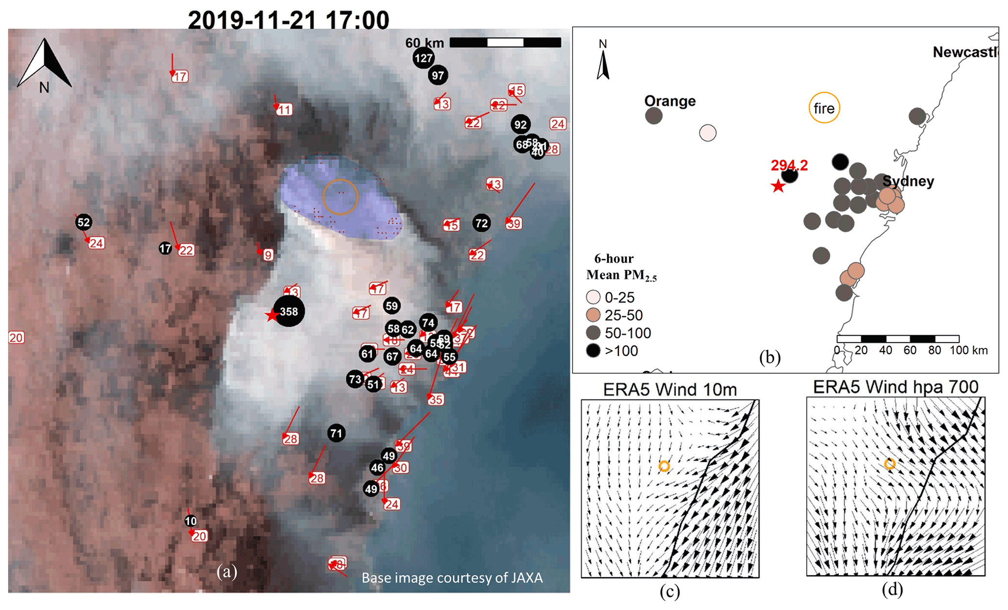
Figure A1Wildfire afternoon. The largest afternoon mean WF PM2.5 was 294.2 µg m−3 at Katoomba AQS, which was the third closest to fire. The fire (Gospers Mountain) eventually burnt ∼ 500 000 ha. A total of 15 other AQSs around the fire had mean PM2.5 > 50. The smoke was flowing mainly to the south over Katoomba (red star) under the surface northerly winds. However, a portion of the smoke was also flowing more easterly with upper-level winds. There is a distinct easterly edge to the smoke plume (a), which appears to align with where the northerly and north-easterly surface winds meet (c). There were widespread PM2.5 exceedances, but only Katoomba recorded values > 150 µg m−3 (b). Smoke from other wildfires to the north of Sydney may have affected the region, indicated by the AQS north of the Gospers fire also recording high PM2.5 values (a). These AQSs are not shown in (b) because they were within 150 km of more than one active fire. In the morning before this image, smoke was flowing directly into Sydney and most AQSs recorded at least one hourly value > 200 µg m−3.
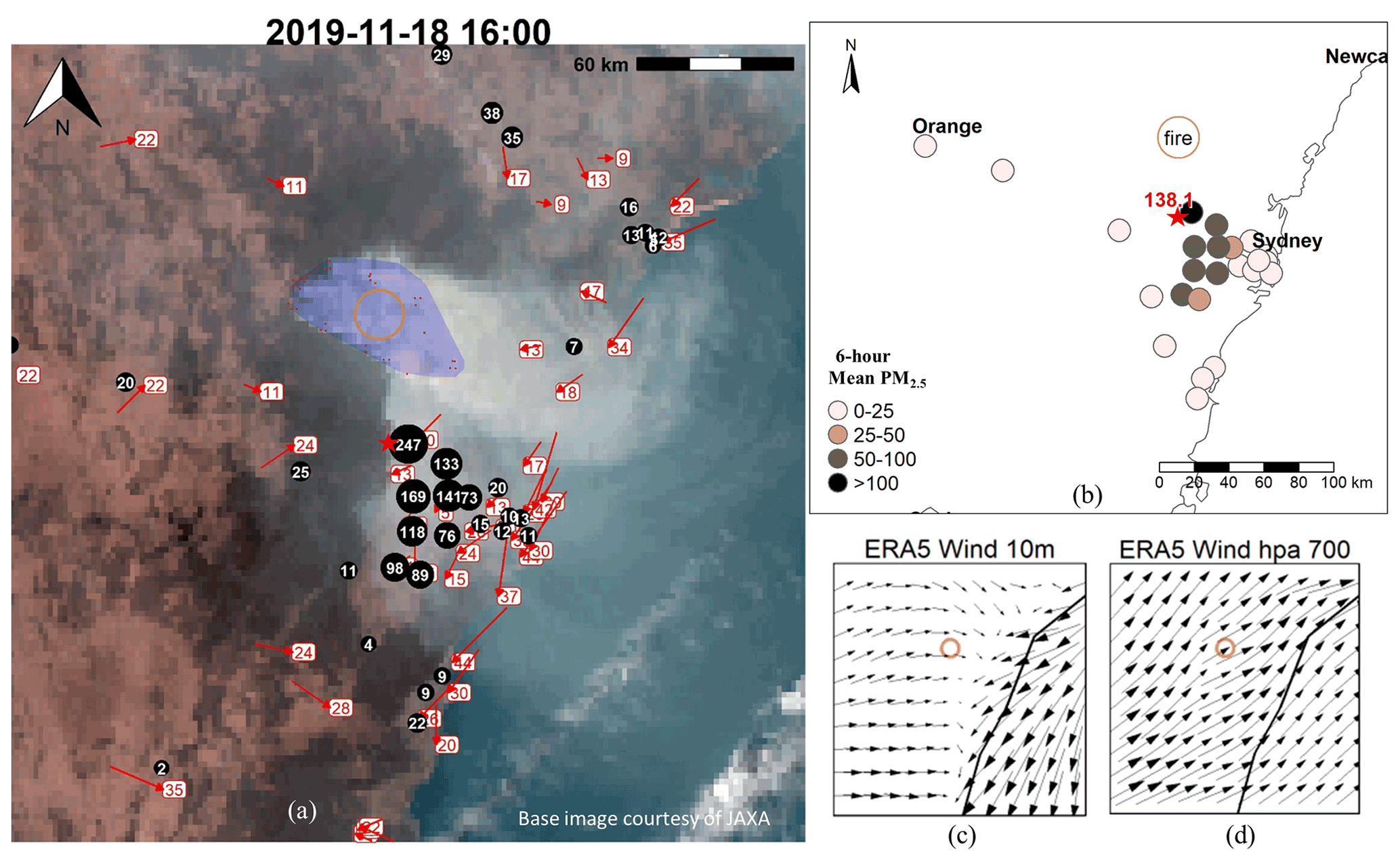
Figure A2Wildfire afternoon 2. The second highest mean afternoon WF PM2.5 was 138.1 µg m−3 at Richmond AQS (red star), which was the closest to the fire at ∼ 50 km. This was also the Gospers Mountain fire. Six other AQSs in the Sydney basin had mean PM2.5 > 50 (b). The smoke flow appears multidirectional (a): to the south with surface winds (c) and to the east with upper-level winds (d). The southerly flow appears to be due to the meeting of surface westerly winds and a NE sea breeze (c). The smoke flowing to the east appears to be above the surface and above the sea breeze as the AQS directly to the east of the fire was under the plume but only recording PM2.5 of 7 µg m−3 (a). The preceding morning had northerly winds blowing smoke directly into Sydney, with several AQSs recording hourly values in the hundreds, so lingering smoke was likely a contributor. This fire burnt through the following night, but PM2.5 levels dropped substantially across Sydney (all < 25 µg m−3) until 02:00 AEST, when PM2.5 increased again (Fig. A4).
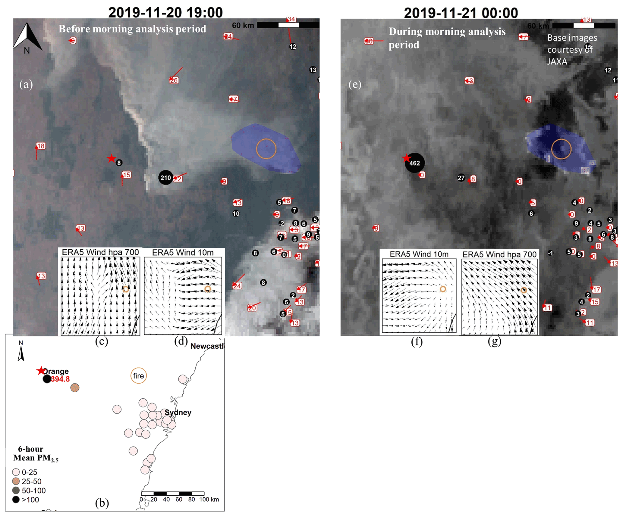
Figure A3Wildfire night. The highest mean night WF PM2.5 was 394.8 µg m−3 at Orange (red star), also from the Gospers Mountain fire. All except one other AQS (Bathurst 25–50 µg m−3) had mean PM2.5 < 25 µg m−3 for this period (b). At midnight (e) the smoke appears to be flowing directly from the fire to Orange (PM2.5 = 462 µg m−3), given no AQSs in Sydney (SE of fire) had high PM2.5 and there were easterly 10 m winds (f). This example shows that smoke circulation can be complex. At 19:00 AEST, 1 h before our “night” period here, there were easterlies at the fire but Orange AQS had southerlies (a). The easterlies had only reached Bathurst (PM2.5 = 210 µg m−3) and not Orange (PM2.5 = 8 µg m−3). Later (e) the easterlies reached Orange along with the surface smoke, resulting in high PM2.5. On the day after this, winds switched to northerlies and PM2.5 rose substantially across Sydney and in Katoomba.
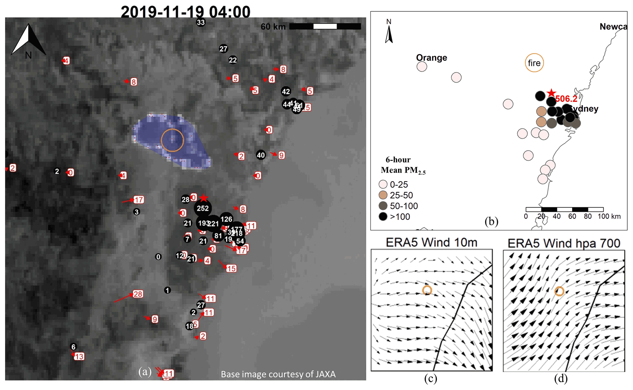
Figure A4Wildfire morning. The highest mean morning WF PM2.5 was 506.2 µg m−3 at Rouse Hill (red star), which was the second closest AQS at 30–40 km from the fire. This was also the Gospers Mountain fire. Richmond AQS was closer but recorded a mean PM2.5 of 112 µg m−3. There were seven other AQSs with a mean > 100 µg m−3 for this period and another three > 50 µg m−3 (b). It is not apparent from the BOM wind (red arrows in a) or the ERA5 data (c, d) that wind flowed directly from the fire to Rouse Hill. The high values may be the result of smoke lingering from the previous day (Fig. A2). However, smoke appeared to clear out during the night period preceding this morning, as the night had comparatively low PM2.5 values (all Sydney AQSs < 25 µg m−3). There may have been drainage flows from the mountains into the Sydney basin that were not captured in the weather data. After this morning, winds turned westerly and then southerly, which pushed smoke away from Sydney and reduced PM2.5 < 25 µg m−3 across Sydney.
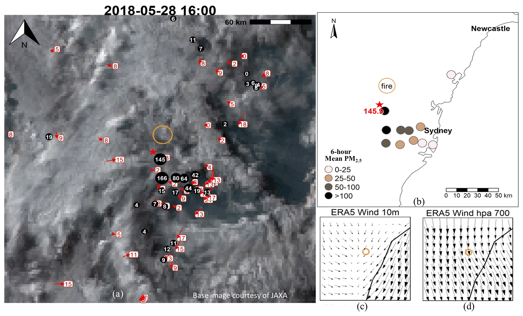
Figure A5HRB afternoon. The highest mean afternoon HRB PM2.5 was 145.9 µg m−3 at the closest AQS in Richmond (red star). Four other AQSs also recorded PM2.5 > 50 µg m−3 during the same period (b). Wind patterns at 10 m (c) suggest that the northerly winds and the meeting of NW and NE winds to the west of the fire funnelled surface smoke to Sydney, similarly to in Fig. A2. Wind speeds were also low (a, c), meaning smoke would have remained in the area for longer. On the morning preceding this period, there was likely some smoke lingering around Sydney because several AQSs recorded hourly values in the twenties and thirties (µg m−3). The synoptic wind direction (d) in the afternoon was northerly, meaning high-level smoke would also have flowed towards Sydney. PM2.5 continued to increase as the day went on and into the night. The highest night mean PM2.5 was also caused by this HRB (Fig. A6).
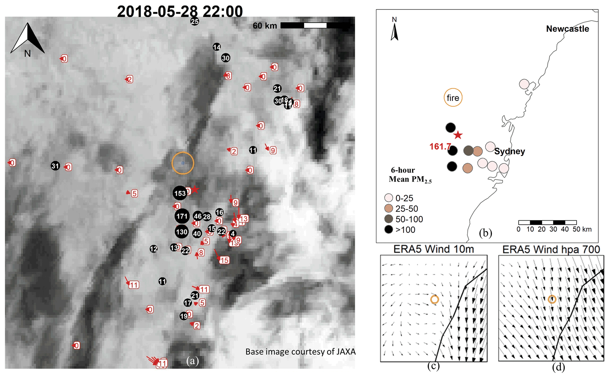
Figure A6HRB night. The highest mean night HRB PM2.5 was 161.7 µg m−3 at the second closest AQS in St Marys (red star), while the closest station was also high (Richmond = 129.4 µg m−3). This highest nighttime PM2.5 for HRBs followed the highest afternoon PM2.5, i.e. the same day and fire (Fig. A5). The high afternoon PM2.5 may have influenced the results this night as 10 m winds were still low (c), suggesting smoke may have lingered from the afternoon. Low wind speeds also meant that any new smoke produced during the night was probably not dispersed. The 10 m winds (c) suggest smoke was not flowing directly from the fire to St Marys, as winds were westerly at the fire. However, the BOM winds (red arrows in a) are zero at Richmond and St Marys at 22:00 AEST, suggesting very calm conditions.
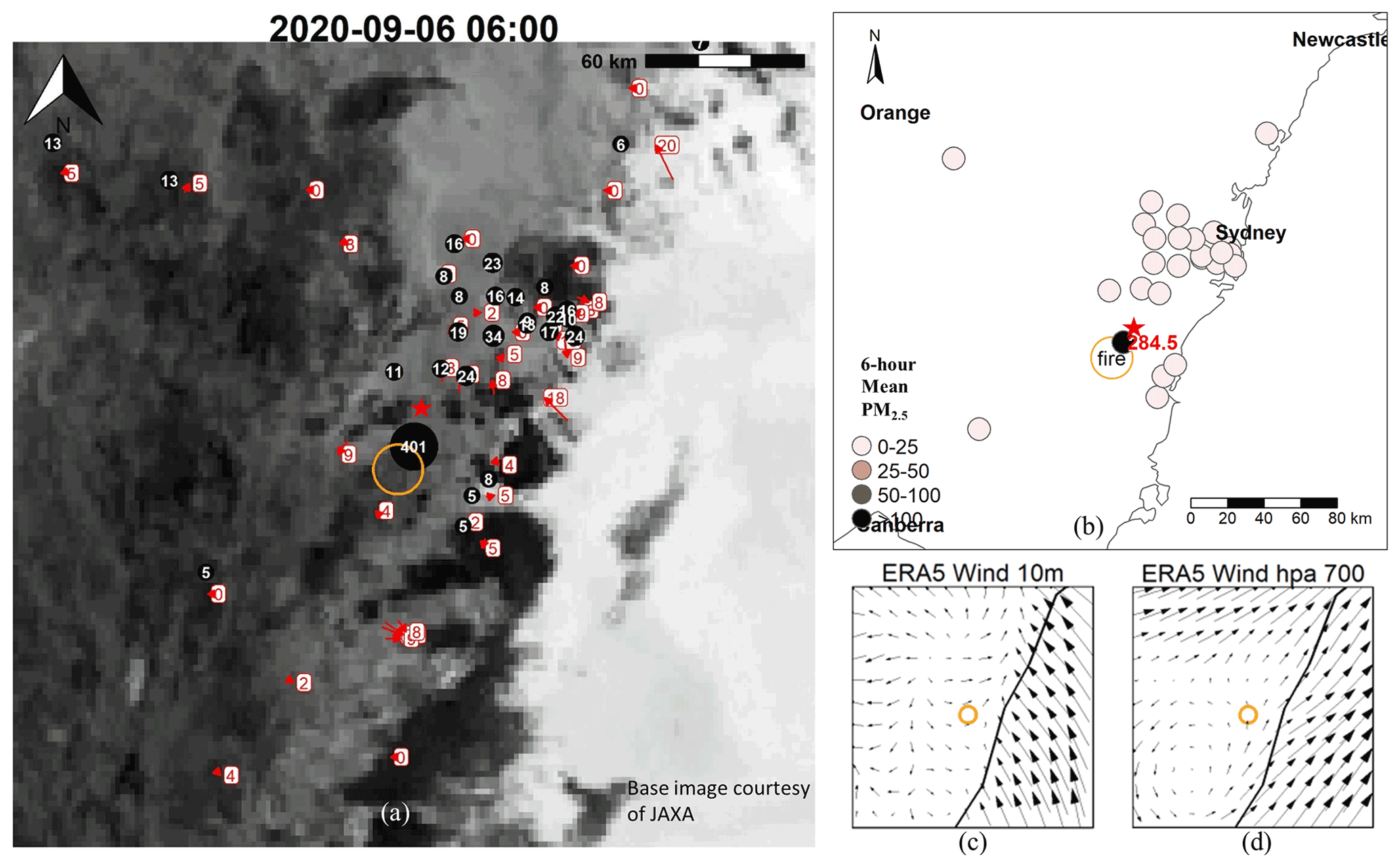
Figure A7HRB morning. The highest mean morning HRB PM2.5 was 284.5 µg m−3 at Bargo AQS (red star) 10 km from the HRB. This example differs from the other panels in that the PM2.5 impact was local only: no other AQSs had > 25 µg m−3 for this morning (b). None of the examples (Figs. A1–A6) had an AQS at such a close distance. The 10 m winds (c) suggest light winds from the fire towards the AQS. The BOM winds near the fire (a) varied in direction but were light. The wind speeds were likely too low to carry smoke far enough north to impact AQSs in Sydney or AQSs in other directions. This HRB was ignited the previous day under W/SW winds but did not noticeably increase PM2.5 at any AQS. On the day after this morning period, strong northerly winds occurred and PM2.5 at Bargo dropped below 10 µg m−3.
VIIRS SNPP hotspots used for analysis are freely available via the NASA FIRMS website at https://firms.modaps.eosdis.nasa.gov/download/ (last access: 1 July 2022; NASA FIRMS, 2022). New South Wales PM2.5 data are freely available from the New South Wales Government online at https://data.airquality.nsw.gov.au/docs/index.html (last access: 1 July 2022; Department of Planning and Environment, 2022). Information on the ERA5 gridded reanalysis weather product download is at https://doi.org/10.24381/cds.bd0915c6 (Hersbach et al., 2018a) and https://doi.org/10.24381/cds.adbb2d47 (Hersbach et al., 2018b).
OFP developed the research aims. MAS and OFP developed the analysis method. MAS ran the statistical analysis and wrote the manuscript. OFP edited the manuscript.
The contact author has declared that neither of the authors has any competing interests.
The results contain modified Copernicus Climate Change Service information 2021. Neither the European Commission nor ECMWF is responsible for any use that may be made of the Copernicus information or data it contains.
Publisher’s note: Copernicus Publications remains neutral with regard to jurisdictional claims in published maps and institutional affiliations.
This article is part of the special issue “The role of fire in the Earth system: understanding interactions with the land, atmosphere, and society (ESD/ACP/BG/GMD/NHESS inter-journal SI)”. It is a result of the EGU General Assembly 2020, 4–8 May 2020.
The authors gratefully acknowledge the financial support of the NSW Department of Planning, Industry and Environment.
This research has been supported by the NSW Department of Planning and Environment through their funding of the NSW Bushfire Risk Management Research Hub.
This paper was edited by Renata Libonati and reviewed by two anonymous referees.
Biau, G. and Scornet, E.: A random forest guided tour, TEST, 25, 197–227, https://doi.org/10.1007/s11749-016-0481-7, 2016.
Boer, M. M., Resco de Dios, V., and Bradstock, R. A.: Unprecedented burn area of Australian mega forest fires, Nat. Clim. Change, 10, 171–172, https://doi.org/10.1038/s41558-020-0716-1, 2020.
Borchers-Arriagada, N., Bowman, D. M. J. S., Price, O., Palmer, A. J., Samson, S., Clarke, H., Sepulveda, G., and Johnston, F. H.: Smoke health costs and the calculus for wildfires fuel management: a modelling study, Lancet Planetary Health, 5, e608–e619, https://doi.org/10.1016/s2542-5196(21)00198-4, 2021.
Bradshaw, S. D., Dixon, K. W., Lambers, H., Cross, A. T., Bailey, J., and Hopper, S. D.: Understanding the long-term impact of prescribed burning in mediterranean-climate biodiversity hotspots, with a focus on south-western Australia, Int. J. Wildland Fire, 27, 643–657, https://doi.org/10.1071/wf18067, 2018.
Broome, R. A., Johnstone, F. H., Horsley, J., and Morgan, G. G.: A rapid assessment of the impact of hazard reduction burning around Sydney, May 2016, Med. J. Australia, 205, 407–408, https://doi.org/10.5694/mja16.00895, 2016.
Chen, G., Guo, Y., Yue, X., Tong, S., Gasparrini, A., Bell, M. L., Armstrong, B., Schwartz, J., Jaakkola, J. J. K., Zanobetti, A., Lavigne, E., Saldiva, P. H. N., Kan, H., Royé, D., Milojevic, A., Overcenco, A., Urban, A., Schneider, A., Entezari, A., Vicedo-Cabrera, A. M., Zeka, A., Tobias, A., Nunes, B., Alahmad, B., Forsberg, B., Pan, S.-C., Íñiguez, C., Ameling, C., Valencia, C. D. la C., Åström, C., Houthuijs, D., Dung, D. V., Samoli, E., Mayvaneh, F., Sera, F., Carrasco-Escobar, G., Lei, Y., Orru, H., Kim, H., Holobaca, I.-H., Kyselý, J., Teixeira, J. P., Madureira, J., Katsouyanni, K., Hurtado-Díaz, M., Maasikmets, M., Ragettli, M. S., Hashizume, M., Stafoggia, M., Pascal, M., Scortichini, M., Coêlho, M. de S. Z. S., Ortega, N. V., Ryti, N. R. I., Scovronick, N., Matus, P., Goodman, P., Garland, R. M., Abrutzky, R., Garcia, S. O., Rao, S., Fratianni, S., Dang, T. N., Colistro, V., Huber, V., Lee, W., Seposo, X., Honda, Y., Guo, Y. L., Ye, T., Yu, W., Abramson, M. J., Samet, J. M., and Li, S.: Mortality risk attributable to wildfire-related PM2.5 pollution: a global time series study in 749 locations, Lancet Planetary Health, 5, e579–e587, https://doi.org/10.1016/S2542-5196(21)00200-X, 2021.
Clarke, H., Tran, B., Boer, M. M., Price, O., Kenny, B., and Bradstock, R.: Climate change effects on the frequency, seasonality and interannual variability of suitable prescribed burning weather conditions in south-eastern Australia, Agr. Forest Meteorol., 271, 148–157, https://doi.org/10.1016/j.agrformet.2019.03.005, 2019.
Cope, M., Keywood, M. D., Emmerson, K., Galbally, I. E., Boast, K., Chambers, S. D., Cheng, M., Crumeyrolle, S., Dunne, E., Fedele, R., Gillett, R., Griffiths, A. D., Harnwell, J., Katzey, J., Hess, D., Lawson, S., Milijevic, B., Molloy, S. B., Powell, J., Reisen, F., Ristovski, Z., Selleck, P. W., Ward, J., Chuanfu, C., and Zeng, J.: Sydney particle study – stage-II, CSIRO Marine and Atmospheric Research, ISBN: 978-1-4863-0359-5, 2014.
Department of Planning and Environment: Air Quality Data API, New South Wales Government, https://data.airquality.nsw.gov.au/docs/index.html, last access: 1 July 2022.
Di Bernardino, A., Iannarelli, A. M., Casadio, S., Pisacane, G., Mevi, G., and Cacciani, M.: Classification of synoptic and local-scale wind patterns using k-means clustering in a Tyrrhenian coastal area (Italy), Meteorol. Atmos. Phys., 134, 30, https://doi.org/10.1007/s00703-022-00871-z, 2022.
Di Virgilio, G., Hart, M. A., and Jiang, N.: Meteorological controls on atmospheric particulate pollution during hazard reduction burns, Atmos. Chem. Phys., 18, 6585–6599, https://doi.org/10.5194/acp-18-6585-2018, 2018.
Emery, C., Liu, Z., Russell, A. G., Odman, M. T., Yarwood, G., and Kumar, N.: Recommendations on statistics and benchmarks to assess photochemical model performance, J. Air Waste Manage., 67, 582–598, https://doi.org/10.1080/10962247.2016.1265027, 2017.
Filkov, A. I., Ngo, T., Matthews, S., Telfer, S., and Penman, T. D.: Impact of Australia's catastrophic 2019/20 bushfire season on communities and environment. Retrospective analysis and current trends, Journal of Safety Science and Resilience, 1, 44–56, https://doi.org/10.1016/j.jnlssr.2020.06.009, 2020.
Fine, P. M., Sioutas, C., and Solomon, P. A.: Secondary Particulate Matter in the United States: Insights from the Particulate Matter Supersites Program and Related Studies, J. Air Waste Manage., 58, 234–253, https://doi.org/10.3155/1047-3289.58.2.234, 2008.
Gill, T.: Woody vegetation cover – Landsat, JRSRP, Australian coverage, 2000–2010, Version 1.0.0, Terrestrial Ecosystem Research Network [data set], https://portal.tern.org.au/metadata/23041 (last access: 10 January 2022), 2012.
Gill, T., Johansen, K., Phinn, S., Trevithick, R., Scarth, P., and Armston, J.: A method for mapping Australian woody vegetation cover by linking continental-scale field data and long-term Landsat time series, Int. J. Remote Sens., 38, 679–705, https://doi.org/10.1080/01431161.2016.1266112, 2017.
Greenwell, B. M.: pdp: an R Package for constructing partial dependence plots, The R J., 9, 421, https://doi.org/10.32614/RJ-2017-016, 2017.
Gupta, P., Christopher, S. A., Box, M. A., and Box, G. P.: Multi year satellite remote sensing of particulate matter air quality over Sydney, Australia, Int. J. Remote Sens., 28, 4483–4498, https://doi.org/10.1080/01431160701241738, 2007.
Haikerwal, A., Akram, M., Sim, M. R., Meyer, M., Abramson, M. J., and Dennekamp, M.: Fine particulate matter (PM2.5) exposure during a prolonged wildfire period and emergency department visits for asthma, Respirology, 21, 88–94, https://doi.org/10.1111/resp.12613, 2016.
Hart, M., De Dear, R., and Hyde, R.: A synoptic climatology of tropospheric ozone episodes in Sydney, Australia, Int. J. Climatol., 26, 1635–1649, https://doi.org/10.1002/joc.1332, 2006.
He, C. R., Miljevic, B., Crilley, L. R., Surawski, N. C., Bartsch, J., Salimi, F., Uhde, E., Schnelle-Kreis, J., Orasche, J., Ristovski, Z., Ayoko, G. A., Zimmermann, R., and Morawska, L.: Characterisation of the impact of open biomass burning on urban air quality in Brisbane, Australia, Environ. Int., 91, 230–242, https://doi.org/10.1016/j.envint.2016.02.030, 2016.
Hersbach, H., Bell, B., Berrisford, P., Biavati, G., Horányi, A., Muñoz Sabater, J., Nicolas, J., Peubey, C., Radu, R., and Rozum, I.: ERA5 hourly data on pressure levels from 1979 to present, Copernicus Climate Change Service (C3S) Climate Data Store (CDS) [data set], https://doi.org/10.24381/cds.bd0915c6, 2018a.
Hersbach, H., Bell, B., Berrisford, P., Biavati, G., Horányi, A., Muñoz Sabater, J., Nicolas, J., Peubey, C., Radu, R., and Rozum, I.: ERA5 hourly data on single levels from 1979 to present, Copernicus Climate Change Service (C3S) Climate Data Store (CDS) [data set], https://doi.org/10.24381/cds.adbb2d47, 2018b.
Hu, X., Belle, J. H., Meng, X., Wildani, A., Waller, L. A., Strickland, M. J., and Liu, Y.: Estimating PM2.5 Concentrations in the Conterminous United States Using the Random Forest Approach, Environ. Sci. Technol., 51, 6936–6944, https://doi.org/10.1021/acs.est.7b01210, 2017.
Jaffe, D., Hafner, W., Chand, D., Westerling, A., and Spracklen, D.: Interannual Variations in PM2.5 due to Wildfires in the Western United States, Environ. Sci. Technol., 42, 2812–2818, https://doi.org/10.1021/es702755v, 2008.
Jiang, N., Scorgie, Y., Hart, M., Riley, M. L., Crawford, J., Beggs, P. J., Edwards, G. C., Chang, L., Salter, D., and Virgilio, G. D.: Visualising the relationships between synoptic circulation type and air quality in Sydney, a subtropical coastal-basin environment, Int. J. Climatol., 37, 1211–1228, https://doi.org/10.1002/joc.4770, 2017.
Johnston, F. H., Henderson, S. B., Chen, Y., Randerson, J. T., Marlier, M., Defries, R. S., Kinney, P., Bowman, D. M., and Brauer, M.: Estimated global mortality attributable to smoke from landscape fires, Environ. Health Persp., 120, 695–701, https://doi.org/10.1289/ehp.1104422, 2012.
Johnston, F. H., Borchers-Arriagada, N., Morgan, G. G., Jalaludin, B., Palmer, A. J., Williamson, G. J., and Bowman, D. M. J. S.: Unprecedented health costs of smoke-related PM2.5 from the 2019–20 Australian megafires, Nature Sustainability, 4, 42–47, https://doi.org/10.1038/s41893-020-00610-5, 2021.
Levy, I., Dayan, U., and Mahrer, Y.: A five-year study of coastal recirculation and its effect on air pollutants over the East Mediterranean region, J. Geophys. Res.-Atmos., 113, D16121, https://doi.org/10.1029/2007JD009529, 2008.
Matz, C. J., Egyed, M., Xi, G., Racine, J., Pavlovic, R., Rittmaster, R., Henderson, S. B., and Stieb, D. M.: Health impact analysis of PM2.5 from wildfire smoke in Canada (2013–2015, 2017–2018), Sci. Total Environ., 725, 138506, https://doi.org/10.1016/j.scitotenv.2020.138506, 2020.
Miller, C., O'Neill, S., Rorig, M., and Alvarado, E.: Air-Quality Challenges of Prescribed Fire in the Complex Terrain and Wildland Urban Interface Surrounding Bend, Oregon, Atmosphere, 10, 515, https://doi.org/10.3390/atmos10090515, 2019.
NASA Fire Information for Resource Management System (Firms), United States Government, https://firms.modaps.eosdis.nasa.gov/download/, last access: 1 July 2022.
NPWS Fire History – Wildfires and Prescribed Burns: https://datasets.seed.nsw.gov.au/dataset/fire-history-wildfires-and-prescribed-burns-1e8b6, last access: 1 January 2022.
Pearce, J. L., Rathbun, S., Achtemeier, G., and Naeher, L. P.: Effect of distance, meteorology, and burn attributes on ground-level particulate matter emissions from prescribed fires, Atmos. Environ., 56, 203–211, https://doi.org/10.1016/j.atmosenv.2012.02.056, 2012.
Price, O. F. and Bradstock, R. A.: The spatial domain of wildfire risk and response in the wildland urban interface in Sydney, Australia, Nat. Hazards Earth Syst. Sci., 13, 3385–3393, https://doi.org/10.5194/nhess-13-3385-2013, 2013.
Price, O. F. and Forehead, H.: Smoke patterns around prescribed fires in Australian eucalypt forests, as measured by low-cost particulate monitors, Atmosphere, 12, 1389, https://doi.org/10.3390/atmos12111389, 2021.
Price, O. F., Williamson, G. J., Henderson, S. B., Johnston, F., and Bowman, D. M. J. S.: The Relationship between Particulate Pollution Levels in Australian Cities, Meteorology, and Landscape Fire Activity Detected from MODIS Hotspots, PLOS ONE, 7, e47327, https://doi.org/10.1371/journal.pone.0047327, 2012.
Price, O. F., Purdam, P. J., Williamson, G. J., and Bowman, D. M. J. S.: Comparing the height and area of wild and prescribed fire particle plumes in south-east Australia using weather radar, J Int. J. Wildland Fire, 27, 525–537, https://doi.org/10.1071/WF17166, 2018.
Price, O. H., Nolan, R. H., and Samson, S. A.: Fuel consumption rates in resprouting eucalypt forest during hazard reduction burns, cultural burns and wildfires, Forest Ecol. Manage., 505, 119894, https://doi.org/10.1016/j.foreco.2021.119894, 2022.
Reid, C. E., Brauer, M., Johnston, F. H., Jerrett, M., Balmes, J. R., and Elliott, C. T.: Critical Review of Health Impacts of Wildfire Smoke Exposure, Environ. Health Persp., 124, 1334–1343, https://doi.org/10.1289/ehp.1409277, 2016.
Reisen, F., Duran, S. M., Flannigan, M., Elliott, C., and Rideout, K.: Wildfire smoke and public health risk, Int. J. Wildland Fire, 24, 1029–1044, https://doi.org/10.1071/WF15034, 2015.
Reisen, F., Meyer, C. P., Weston, C. J., and Volkova, L.: Ground-Based Field Measurements of PM2.5 Emission Factors From Flaming and Smoldering Combustion in Eucalypt Forests, J. Geophys. Res.-Atmos., 123, 8301–8314, https://doi.org/10.1029/2018JD028488, 2018.
Rodriguez-Galiano, V., Sanchez-Castillo, M., Chica-Olmo, M., and Chica-Rivas, M.: Machine learning predictive models for mineral prospectivity: An evaluation of neural networks, random forest, regression trees and support vector machines, Ore Geol. Rev., 71, 804–818, https://doi.org/10.1016/j.oregeorev.2015.01.001, 2015.
Saide, P. E., Peterson, D. A., da Silva, A., Anderson, B., Ziemba, L. D., Diskin, G., Sachse, G., Hair, J., Butler, C., Fenn, M., Jimenez, J. L., Campuzano-Jost, P., Perring, A. E., Schwarz, J. P., Markovic, M. Z., Russell, P., Redemann, J., Shinozuka, Y., Streets, D. G., Yan, F., Dibb, J., Yokelson, R., Toon, O. B., Hyer, E., and Carmichael, G. R.: Revealing important nocturnal and day-to-day variations in fire smoke emissions through a multiplatform inversion, Geophys. Res. Lett., 42, 3609–3618, https://doi.org/10.1002/2015gl063737, 2015.
Schroeder, W., Oliva, P., Giglio, L., and Csiszar, I. A.: The New VIIRS 375m active fire detection data product: Algorithm description and initial assessment, Remote Sens. Environ., 143, 85–96, https://doi.org/10.1016/j.rse.2013.12.008, 2014.
Shah, S. U., Yebra, M., Van Dijk, A. I. J. M., and Cary, G. J.: A New Fire Danger Index Developed by Random Forest Analysis of Remote Sensing Derived Fire Sizes, Fire, 5, 152, https://doi.org/10.3390/fire5050152, 2022.
Specht, R. L. and Specht, A.: Australian plant communities: dynamics of structure, growth and biodiversity, Oxford University Press, South Melbourne, 492 pp., ISBN-10.019553705X; ISBN-13.978-0195537055, 1999.
Storey, M. A. and Price, O. F.: Prediction of air quality in Sydney, Australia as a function of forest fire load and weather using Bayesian statistics, PLOS ONE, 17, e0272774, https://doi.org/10.1371/journal.pone.0272774, 2022.
Strobl, C., Boulesteix, A.-L., Kneib, T., Augustin, T., and Zeileis, A.: Conditional variable importance for random forests, BMC Bioinformatics, 9, 307, https://doi.org/10.1186/1471-2105-9-307, 2008.
Volkova, L., Meyer, C. P. M., Murphy, S., Fairman, T., Reisen, F., and Weston, C.: Fuel reduction burning mitigates wildfire effects on forest carbon and greenhouse gas emission, J Int. J. Wildland Fire, 23, 771–780, https://doi.org/10.1071/WF14009, 2014.
Wang, T., Du, H., Zhao, Z., Russo, A., Zhang, J., and Zhou, C.: The impact of potential recirculation on the air quality of Bohai Bay in China, Atmos. Pollut. Res., 13, 101268, https://doi.org/10.1016/j.apr.2021.101268, 2022.
Wright, M. N. and Ziegler, A.: ranger: A Fast Implementation of Random Forests for High Dimensional Data in C++ and R, J. Stat. Softw., 77, 1–17, https://doi.org/10.18637/jss.v077.i01, 2017.
Wright, M. N., Ziegler, A., and König, I. R.: Do little interactions get lost in dark random forests?, BMC Bioinformatics, 17, 145, https://doi.org/10.1186/s12859-016-0995-8, 2016.
Yao, J., Brauer, M., and Henderson, S. B.: Evaluation of a Wildfire Smoke Forecasting System as a Tool for Public Health Protection, Environ. Health Persp., 121, 1142–1147, 2014.
Yimin, M. and Lyons, T. J.: Recirculation of coastal urban air pollution under a synoptic scale thermal trough in Perth, Western Australia, Atmos. Environ., 37, 443–454, https://doi.org/10.1016/S1352-2310(02)00926-3, 2003.
Zeng, T., Wang, Y. H., Yoshida, Y., Tian, D., Russell, A. G., and Barnard, W. R.: Impacts of Prescribed Fires on Air Quality over the Southeastern United States in Spring Based on Modeling and Ground/Satellite Measurements, Environ. Sci. Technol., 42, 8401–8406, https://doi.org/10.1021/es800363d, 2008.