Mass flows, turbidity currents and other hydrodynamic consequences of small and moderate earthquakes in the Sea of Marmara

Earthquake-induced submarine slope destabilization is known to cause mass wasting and turbidity currents, but the hydrodynamic processes associated with these events remain poorly understood. Instrumental records are rare, and this notably limits our ability to interpret marine paleoseismological sedimentary records. An instrumented frame comprising a pressure recorder and a Doppler recording current meter deployed at the seafloor in the Sea of Marmara Central Basin recorded the consequences of a M_w 5.8 earthquake occurring on 26 September 2019 and of a M_w 4.7 foreshock 2 d before. The smaller event caused sediment resuspension and weak current (<4 cm s⁻¹) in the water column. The larger event triggered a complex response involving a debris flow and turbidity currents with variable velocities and orientations, which may have resulted from multiple slope failures. A long delay of 10 h is observed between the earthquake and the passing of the strongest turbidity current. The distance traveled by the sediment particles during the event is estimated to have extended over several kilometers, which could account for a local deposit on a sediment fan at the outlet of a canyon (where the instrument was located), but the sedimentation event did not likely cover the whole basin floor. We show that after a moderate earthquake, delayed turbidity current initiation may occur, possibly by ignition of a cloud of resuspended sediment.

1 Introduction

Triggering of mass wasting and turbidity currents by earthquakes is a hazard that can damage seafloor infrastructure (Heezen et al., 1954) and may enhance co-seismic tsunami generation (Okal and Synolakis, 2001; Synolakis et al., 2002; Hébert et al., 2005; Özeren et al., 2010). Earthquake-triggered canyon flushing is also a primary driver of submarine canyon development and material transfer from seismically active continental margins to the deep ocean (Mountjoy et al., 2018). It is often considered that a peak ground acceleration (PGA) on the order of 0.1 g is needed for an earthquake to trigger a submarine slope failure (Dan et al., 2009; Nakajima and Kanai, 2000). A peak ground velocity threshold of 16–25 cm s⁻¹ for turbidity current triggering has been proposed based on observations after the 4 November 2016 Kaikōura, New Zealand, M_w 7.8 earthquake (Howarth et al., 2021). The corresponding peak ground acceleration cannot be accurately determined because the seismic waveform in this study was modeled at long periods (>2 s). Nevertheless, strong motion records from this earthquake suggest this peak ground velocity threshold does correspond to a peak ground acceleration on the order of 0.1 g (Bradley et al., 2017). On the other hand, a global compilation of cable breaks shows that mass flows have been triggered by individual earthquakes of M_w as low as 3.1 (with estimated PGA ≈ 10⁻³ g), while on other margins where sediment input is relatively low and/or earthquakes frequent, M_w>7 earthquakes failed to trigger cable breaking flows (Pope et al., 2017). In the Mediterranean region, the threshold is reportedly around M_w=5.

In spite of this high regional variability, turbidite deposits in several seismically active zones have been used as paleoseismological event markers (e.g., Adams, 1990; Goldfinger et al., 2003, 2012; McHugh et al., 2014; Ikehara et al., 2016; Polonia et al., 2016). For instance, Holocene turbidite records in the Sea of Marmara basins display a recurrence of 200 to 300 years, which roughly corresponds to the recurrence interval of M_w>6.8 earthquakes (McHugh et al., 2006, 2014; Drab et al., 2012, 2015; Yakupoğlu et al., 2019). Synchronicity of turbidites over a large area is considered the most robust criterion for recognizing sedimentary events caused by large earthquake ruptures, although this approach has caveats (Talling, 2021; Atwater et al., 2014). Distinguishing seismoturbidites, caused by earthquakes and related mass-wasting events, and turbidites resulting from other processes (e.g., floods, storms, sediment loading) from their sedimentological characteristics is particularly challenging (Talling, 2021; Heerema et al., 2022). Seismoturbidites generally comprise a basal silt–sand bearing layer under a layer of apparently homogenous mud (named homogenite or tail) with small or gradual, if any, variations in grain size and chemical composition (Polonia et al., 2017; McHugh et al., 2011; Çağatay et al., 2012; Eriş et al., 2012; Gutierrez-Pastor et al., 2013; Nakajima and Kanai, 2000; Beck et al., 2007). The grain size break between turbidite and homogenite layers is however not specific to seismoturbidites and can result from mud settling processes commonly occurring in turbidity currents (e.g., Talling et al., 2012). In lakes and closed basins several other characteristics of turbidite–homogenites, such as the alternation of silt–sand and mud laminae within a single turbidite unit and presence of bi-directional cross-bedding or flaser bedding have been interpreted as indicators of deposition from oscillatory currents associated with seiches or turbidity current reflection (Beck et al., 2007; Çağatay et al., 2012; McHugh et al., 2011). Indeed, internal tsunami waves and turbidity current reflection have been recorded after landslides in lakes (Brizuela et al., 2019). However, seismoturbidites on ocean margins have fairly similar characteristics to those in closed basins, but their layering has been interpreted differently, as a consequence of confluence (stacked or amalgamated turbidites) or current speed variations (multi-pulsed turbidites) (Gutierrez-Pastor et al., 2013; Nakajima and Kanai, 2000; Goldfinger et al., 2003). There is currently a lack of in situ instrumental records that could substantiate inferred hydrodynamic processes.

Monitoring experiments have generated observations of turbidity currents flowing in submarine canyons and initiated by meteorological events, seasonal discharge from rivers and occasionally by landslides (Xu et al., 2004, 2010; Puig et al., 2004; Palanques et al., 2008; Liu et al., 2012; Khripounoff et al., 2012; Hughes Clarke, 2016; Gwyn Lintern et al., 2016; Azpiroz-Zabala et al., 2017; Paull et al., 2018; Hage et al., 2019; Normandeau et al., 2020; Heerema et al., 2022). Some turbidity currents originating from sediment remobilization events are driven by a thick dense basal layer, which is able to displace and bury heavy instruments (Paull et al., 2018). On the other hand, progressive or pulsed buildup of turbidity current energy is considered typical of hyperpycnal flows initiated by river floods (Mulder et al., 2003; Khripounoff et al., 2012). However, the hydrodynamic characteristics of turbidity currents resulting from landslides and floods may not systematically differ, especially when observations are done at a distance from the source (Heerema et al., 2022). Most information on earthquake-triggered events is still indirect, based on cable ruptures (e.g., Gavey et al., 2017; Pope et al., 2017; Hsu et al., 2008), geomorphological and sedimentological observations (Mountjoy et al., 2018; Cattaneo et al., 2012; Piper et al., 1999), and information from displaced instruments (Garfield et al., 1994). In Japan, in situ records of pressure and temperature were obtained from displaced ocean bottom seismometers (OBSs) after the 2011 Tohoku M_w 9.1 earthquake (Arai et al., 2013) and from cabled observatories after the 2003 Tokachi-Oki M_w 8.3 earthquake (Mikada et al., 2006) and after a moderate (M 5.4) earthquake off of Izu Peninsula (Kasaya et al., 2009). After the large events, strong bottom currents of more than 1 m s⁻¹ were implied, generally starting 2–3 h after the earthquake, with no indication of oscillation or pulsing. In the case off of Izu a mudflow was observed with a camera 5 min after the earthquake and was followed 15 min later by a change in current direction and speed.

We here present results from an instrumental deployment at the seafloor that accidentally recorded the consequences of earthquakes that occurred on 24 and 26 September 2019 in the Sea of Marmara with magnitudes of M_w 4.7 and 5.8 respectively (Fig. 1a). The pressure, temperature and current records from this single instrument demonstrate that both events caused sediment resuspension in turbid clouds, but only the larger event triggered turbidity currents. However, the instrument suffered a rather complex sequence of disturbances, and a 10 h delay is observed between the earthquake and peak current recording. Here, we propose a scenario which could explain the observations and discuss their implications for the understanding of seismoturbidite records.

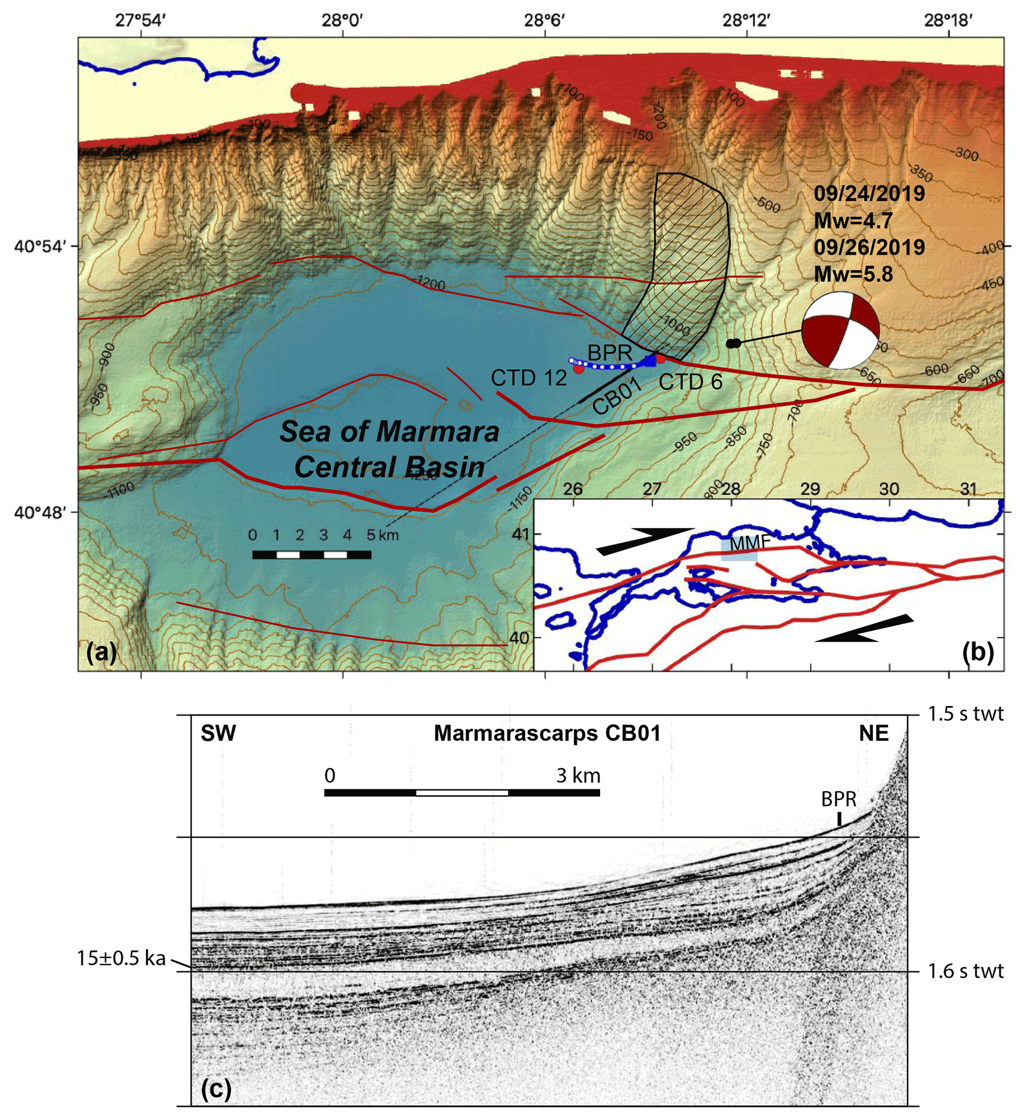
Figure 1 Context of instrumental deployment. (a) Bathymetric map of the Sea of Marmara Central Basin with simplified fault geometry (in red). The hatched zone is a suspected mass-wasting zone (Zitter et al., 2012). Location of instrumented frame comprising bottom pressure recorder (BPR) and Doppler current meter is indicated by blue square. The blue banana-shaped line with white dots represents the calculated trajectory of a sedimentary particle during the waning phase of the turbidity current. Red dots are conductivity–temperature–depth (CTD) profiles 6 and 12 shown in Fig. S1. Epicenter location of earthquakes and the focal mechanism of the main shock are indicated. (b) Location of study area. North Anatolian Fault system is shown in red. MMF is the Main Marmara Fault. (c) Sediment sounder profile from Marmarascarps cruise (Armijo and Malavieille, 2002). Indicative age of reflector from Beck et al. (2007). The instrument (BPR) was deployed on a depositional fan at the base of slope and canyon outlet that differ in seismic character from the reflector sequence in the basin.

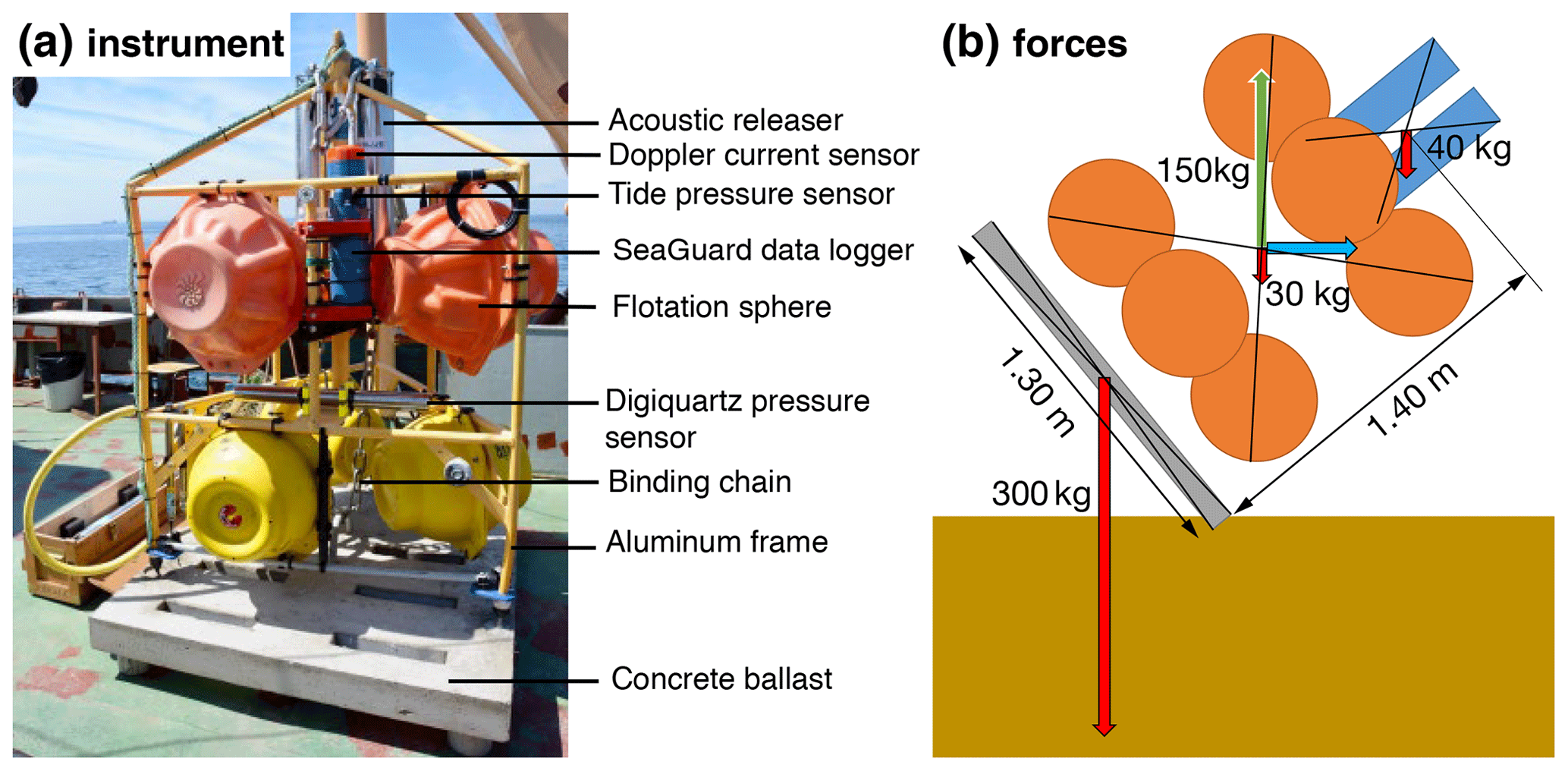
Figure 2 Instrumented frame. (a) Photo of the instrumented frame before deployment. (b) Sketch showing forces applied to the elements of the instrumented frame in water. The red arrows represent the weight in water of the cement ballast, of the instrumented frame and of the acoustic release system on top. The green arrow represents the buoyancy of the flotation spheres. The blue arrow represents the current drag, which depends on current speed and instrument tilt.

2 Context and data collection

A series of instrumental deployments was planned to record naturally occurring resonant water column oscillations (seiches) at various locations in the Sea of Marmara with the aim to improve tsunami models (Henry et al., 2021). An instrumented frame was thus deployed at 40.8568^∘ N, 28.1523^∘ E and 1184 m water depth in the Central Basin on 9 May 2019 and recovered 6 months later (19 November 2019) (Fig. 1a). This site is located at the outlet of a complex canyon system with multiple confluence points and tributaries originating from the edge of the continental shelf (Fig. 1). Sediment sounder profiles indicate a depositional fan or lobe is present at this location (Fig. 1c). Canyons observed on the relatively steep sedimented slope (≈10^∘) of the deep basins of the Sea of Marmara are presumably fed by mass flows sourced from the canyon heads and walls (Zitter et al., 2012; Çagatay et al., 2015). In addition, the slope west of the canyons immediately north of the deployment site hosts a landslide covering about 24 km², and cores taken at the base of the slope contain a sandy debris flow deposit of 35–40 cm thickness buried 2 m below the seafloor (Zitter et al., 2012). The Main Marmara Fault (MMF, Fig. 1b) is defined as the part of the northern branch of the North Anatolian Fault system crossing the Sea of Marmara (Le Pichon et al., 2001, 2003). A splay of the MMF runs along the base of this slope (Armijo et al., 2002; Grall et al., 2012; Şengör et al., 2014). The 24 and 26 September 2019 earthquakes occurred under the canyon system, and their epicenters are located 5 km east-northeast of the instrument, less that 500 m apart (Fig. 1). The rupture occurred within the crust at 9–13 km depth on a northward-dipping fault located north of the principal displacement zone of the Main Marmara Fault. The focal mechanism indicate a right-lateral strike-slip motion with a reverse component (Karabulut et al., 2021). The rupture neither reached the seafloor nor caused a tsunami. For instance, tidal gauge records obtained at Marmara Ereğlisi do not deviate more than 1 hPa from a fitted tidal model.

The instrumentation on the frame comprises (1) an RBR bottom pressure recorder (BPR) with a Paroscientific 0–2000 m Digiquartz pressure and temperature sensor and (2) a SeaGuard recording current meter (RCM) equipped with a ZPulse 4520 Doppler current sensor operating in the 1.9–2 MHz frequency range and other sensors, including temperature, pressure (tide sensor, Aanderaa 5217), conductivity (Aanderaa 4319) and oxygen (optode, Aanderaa 4330) (Fig. 2). The RBR pressure and temperature recording interval was set to 5 s, and that of the SeaGuard RCM was set to 1 h for all sensors. The SeaGuard instrument was fixed on the upper part of the frame, and sensors were 1.5 m above the seafloor. The ZPulse Doppler current sensor is a single-point current sensor, not an acoustic Doppler profiler (ADCP). It emits four narrow (2^∘) beams paired in opposite directions along two orthogonal axes in a plane (parallel to the seafloor if the frame is standing upright) and measures Doppler backscatter in cells extending 0.5–2 m from the instrument (Fig. 3). The Doppler current sensor was set in burst mode, averaging 150 pings taken every second at the end of each 1 h recording interval, and in forward ping mode so that only data from sensors measuring a positive Doppler shift, upstream currents moving toward the instrument, are used to calculate current speed. The tide sensor is a piezoresistive sensor with a specified accuracy comparable to that of the Digiquartz sensors (4 kPa for a 0–2000 m sensor vs. 2 kPa for a Digiquartz sensor with the same range) and 0.2 hPa (2 mm ocean depth) resolution and comprises a temperature sensor of 0.2 ^∘C accuracy and 0.001 ^∘C resolution. The tide sensor averages pressure measured at a 2 Hz sampling rate over 300 s at the end of each 1 h time interval. The tide sensor was checked against an atmospheric reference between deployments and found to have a minimal drift, less than 1 hPa. The main purpose of the pressure sensor records was to detect long period variations in water height, related for instance to tides and seiche oscillations but also sensitive to pressure variations caused by P waves. In addition, Digiquartz sensors are intrinsically sensitive to acceleration but, to a small extent, 160 hPa g⁻¹ for an instrument with 20 MPa range according to the calibration report.

Figure 3 Reconstruction of frame position based on instrument tiltmeter and compass data: (a) before the earthquake; (b) tilted, between 25 min and 10.5 h after earthquake; and (c) back in nearly upright position 11 h after earthquake. Position of Digiquartz pressure sensor (black circle), Aanderaa tide sensor (red circle) and Doppler current meter beam cells (green segments).

As we will show that the 24 September 2019 earthquake caused the instrumented device to lay on its side for several hours and then straighten up, understanding the setup of the seafloor device and its stability is important (Fig. 2b). The frame is made of aluminum and has six rigidly bound flotation spheres of 25 kg buoyancy each. The net weight of the instrumented frame in water is −80 kg. The frame is rigidly attached to a 12 cm thick 1.5×1.3 m concrete slab, weighing 300 kg in water. The assembly of the heavy slab and buoyant frame is stable in an upright position in the water and on the seafloor. Moreover, it is estimated that a current of 1 m s⁻¹ would cause a total horizontal drag of 75 kg (≈750 dN) when the device is in an upright position, which is insufficient to destabilize it. If a stronger current or other external forces cause the assembly to tilt and lay on one side, the moment of the gravity and buoyancy forces should straighten the device back to an upright position when these external forces are removed.

Measurement of current speed and direction by a tilted instrument is a related issue that we here consider. The orientation and attitude of the SeaGuard RCM is measured with a two-component accelerometer and a magnetic compass, and the recorded data include tilt in the x and y directions and the heading of the x axis. Tilt x and y components are factory calibrated from −35 to +35^∘ with an accuracy of 1.5^∘. Tests performed in the laboratory (see Fig. S1 in the Supplement) showed that tilt information remains consistent outside this range, even when the instrument is upside down. Tilt measurements are accurate within 3^∘ up to 60^∘ but saturate at about 80^∘ (Fig. S2). Uncertainty on heading also increases with tilt, especially when the instrument is tilted toward the x direction. However, measured heading remains ±20^∘ of true heading for a tilting of up to 60^∘ (Fig. S3). The current measured in the instrument plane is corrected for tilt assuming current is horizontal. As far as this approximation is valid, the current record should in principle remain fairly accurate when the instrument is tilted beyond the normal range of operation (±35^∘) and at least to 60^∘. However, the compass was not calibrated for an upside-down configuration. If the top of the instrument would happen to be oriented downward, the measured current direction will be unreliable, even though the absolute speed may still be correctly estimated. Another problem may arise if one of the Doppler sensors is facing down into the sediment so that its measurement cell is below the seafloor. If the sensor pointing upward in the opposite direction is recording a negative Doppler shift, this value will be ignored in the forward ping mode. In this case, the measurement retained to calculate current velocity will correspond to noise from the sensor facing toward the seafloor. In all situations, it remains possible to recalculate the sensor readings retained by the calculator from the current velocity and orientation parameters recorded by the instrument by projecting the velocity vector back into the instrument plane and thus assessing the reliability of data.

The strength of the backscattered signal can be used as a proxy for turbidity. The ZPulse emits in the 1.9–2 MHz band, corresponding to a wavelength (λ) of 750 µm. Doppler backscatter current meters have maximum sensitivity for particles of diameter $D=\mathit{\lambda }/\mathit{\pi }$ and can detect particles down to diameter D=0.08λ, for which backscatter power is less than $\mathrm{1}/\mathrm{10}$ of peak backscatter power (Guerrero et al., 2011, 2012). The SeaGuard RCM should thus be mostly sensitive to the presence in suspension of larger than 63 µm. This, however, does not imply that the detected particles are all sand grains in the mineralogical sense, as clay flocs of the same size also cause backscattering.

3 Results

3.1 Pressure and tilt records

Small earthquakes are detected as pressure spikes, while oscillations are recorded after large earthquakes. The 24 September 2019 M_w 4.7 earthquake caused a short pressure transient of 25 hPa at 08:00:26 GMT followed by small pressure oscillations of less than 3 hPa amplitude decaying over a few minutes. The seismic wave train from the 26 September 2019 M_w 5.8 earthquake is recorded by the Digiquartz pressure sensor as oscillations, initiated by a pressure drop of 65 hPa between 10:59:22 and 10:59:26 GMT (Fig. 4). For the sampling interval of 5 s used in this setup, the recorded signal is aliased, which precludes quantitative interpretation in terms of velocity or acceleration. However, the initial pressure drop after the 26 September 2019 earthquake may indicate a negative polarity of the first P-wave arrival at the instrument site, located on an ascending ray path.

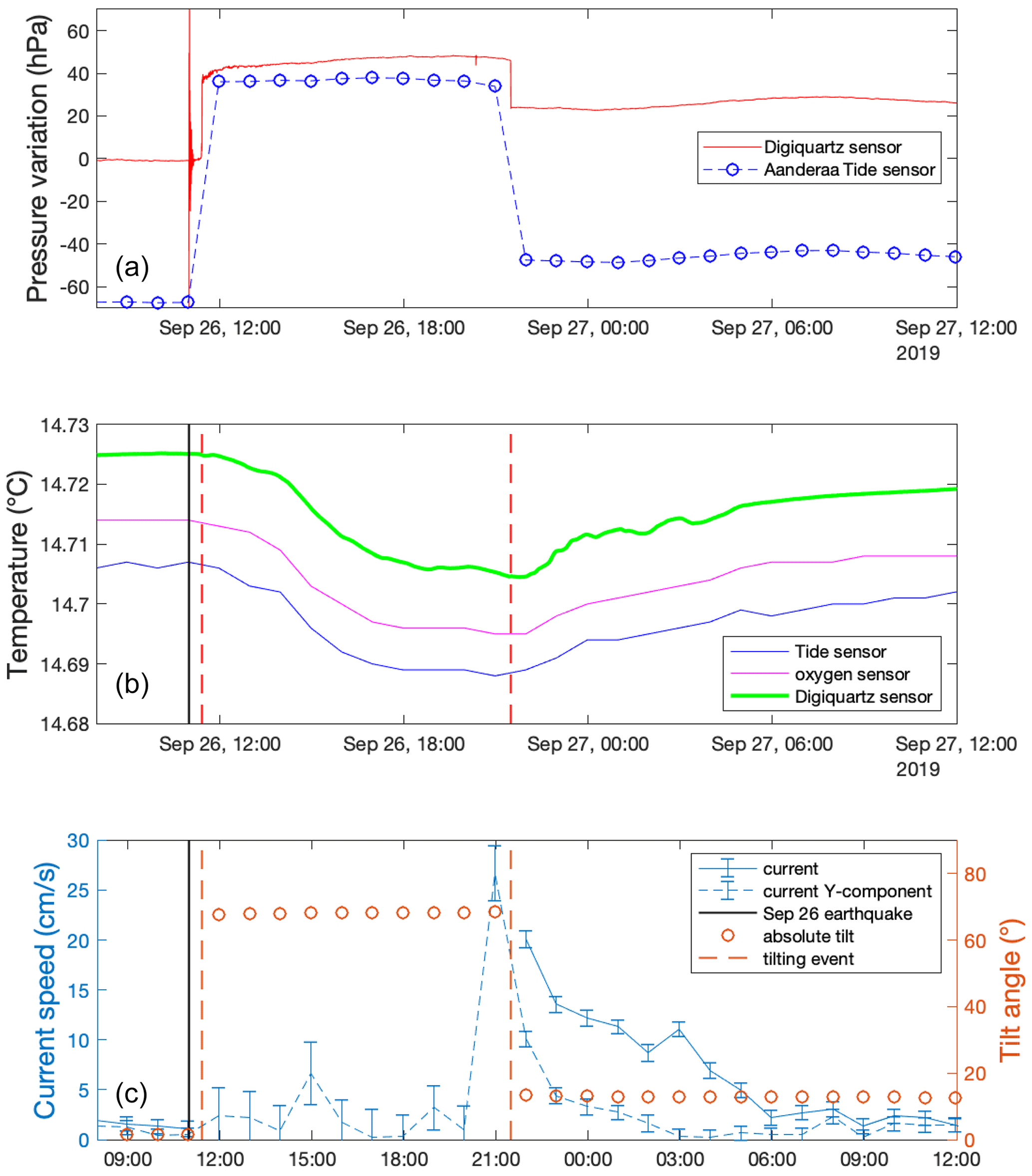
Figure 4 Time series around the time of occurrence of a M_w 5.8 earthquake: (a) pressure variations recorded by two instruments on the instrumented frame; (b) temperature records from Digiquartz, tide and oxygen sensors; and (c) current and tilt data recorded by a SeaGuard RCM. Between the tilting events only one component of the Doppler current meter functioned reliably (y component oriented N 200^∘) and is here reported.

A total of 25 min after the M_w 5.8 earthquake, a new disturbance of the pressure sensor is observed at 11:23:41 GMT. The pressure then progressively increases by 30.9 hPa in 15 s between 11:24:46 and 11:25:01 GMT before stabilizing. Over the corresponding 1 h time interval between successive records, the SeaGuard RCM, initially subvertical (tilt less than 2^∘), acquires a strong tilt (Fig. 3). At 11:57:48 GMT, measured tilt is −65^∘ along the x axis and +19^∘ along the y axis, with the x axis in a N 161^∘ azimuth. These values remain constant ±2^∘ over the next 10 h, corresponding to an absolute tilt of 68^∘ (Fig. 4). The tilting of the instrument causes the Digiquartz and tide sensors to record different pressure variations because they are located at different positions on the frame (Fig. 2). Moreover, the pressure readings by the Digiquartz sensor also depend on its orientation relative to Earth's gravity. Pressure at the tide sensor location increases about 100 kPa, corresponding to a 1 m drop and indicating that the frame was then practically laying on its side; 10 h later, the device apparently straightens itself in about 5 s, between 21:28:29 and 21:28:34 GMT as indicated by a rapid pressure variation. After that, the recorded tilt parameters are moderate and stabilize at −11.5^∘ for the x axis and 5.3^∘ for the y axis, with the x axis in a N 105.3^∘ azimuth.

Baseline changes before and after the earthquake correspond to an increase of 23 hPa for the Digiquartz sensor and 20 hPa for the tide sensor. These concur that the instrumented frame was about 20 cm deeper after returning to upright position. Considering that the slope at the location of the instrument is about 1 %, this may correspond to a 20 m lateral downslope displacement. However, in the absence of other information, it is not known whether the pressure baseline change is a consequence of instrument lateral displacement or burial in place.

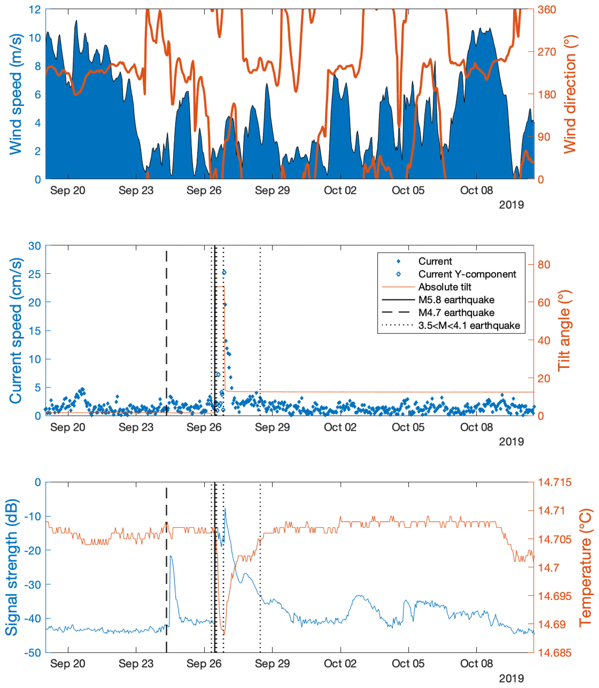
Figure 5 Time series acquired with a SeaGuard RCM during the September 2019 seismicity cluster and ERA5 reanalyzed meteorological data (Hersbach et al., 2018): ERA5 wind data (top panel), current speed and tilt (middle panel), and backscatter signal strength and temperature (bottom panel).

The M_w 4.7 earthquake caused minor disturbances of the attitude of the instrument, with variations in tilt and heading of less than 0.5^∘. A M_w 3.6 foreshock of the M_w 5.8 earthquake occurring on 26 September 2019 at 07:32 GMT also caused minor disturbances. These indicate that the seafloor was sensitive to ground shaking caused by these small earthquakes. However, this did not cause the device to sink into the sediment. Changes in the pressure baseline of the Digiquartz sensor between before and after these earthquakes are difficult to resolve and correspond to less than 5 mm vertical displacement for the first event and less than 2 mm for the second one.

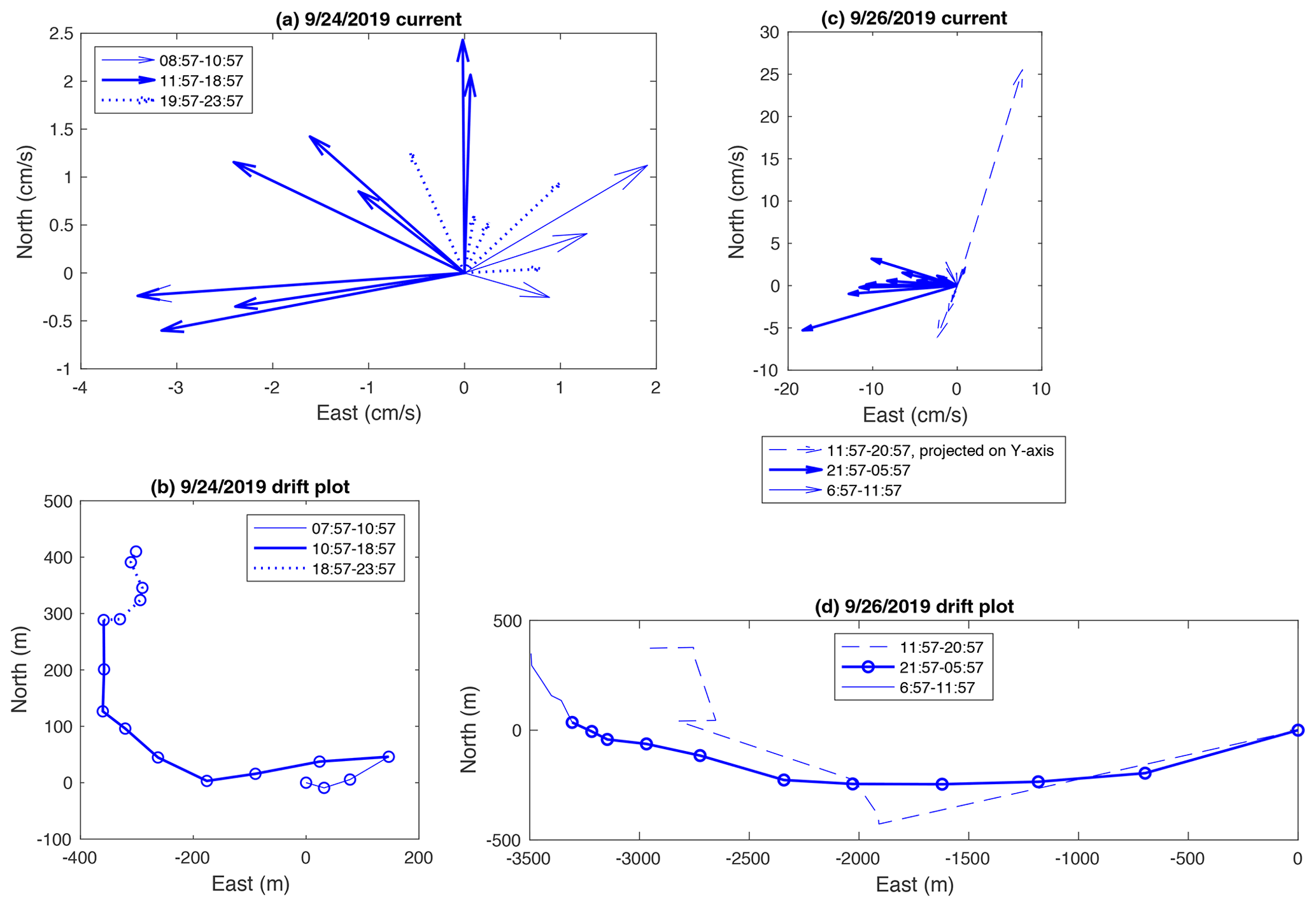
Figure 6 Current recorded after M_w 4.7 and M_w 5.8 earthquakes: (a) current velocity arrows recorded every hour between 08:57 and 23:57 GMT on 24 September 2019; (b) drift plot over the same time interval, with the change in current direction and strength between 10:57 and 11:57 GMT coinciding with increasing backscatter strength (see Fig. 4), indicative of increased turbidity; and (c) current velocity arrows recorded every hour between 12:00 GMT on 26 September 2019 and 06:00 GMT on 27 September 2019. Dashed arrows show measurements acquired in the y direction when the instrument was strongly tilted (Fig. 3b), and plain arrows show when it was back in an upright position (Fig. 3c). (d) Drift plot over the same time interval, with the dashed part corresponding to the strongly tilted position.

3.2 Current records

The 24 September 2019 M_w 4.7 earthquake was followed by a small increase in current strength peaking at 3.4 cm s⁻¹ at noon, 4 h after the earthquake (Fig. 5). Comparable events in terms of duration and strength occurred spontaneously on 20 September 2019 (with currents up to 4.7 cm s⁻¹) and 26 September 2019 (with currents up to 3.3 cm s⁻¹) just before the M_w 5.8 earthquake. During all three events the dominant current was from the east, thus coming from the direction of the canyon, but there is an important difference between the event that occurred after the M_w 4.7 earthquake and the two others. During that event a change in current direction occurred from eastward to westward between 10:57 and 11:57 GMT, while the current strength increased from 2.2 cm s⁻¹ to its peak value of 3.4 cm s⁻¹ (Fig. 6). During the other events, buildup was more progressive and did not involve a change in direction. A drift plot, calculated by summing velocity vectors over time, reproduces the motion of a particle assuming a uniform velocity field (Fig. 6). The total drift occurring in the 8 h following the current inversion is about 500 m. Current direction varies from westward to northward during this time interval.

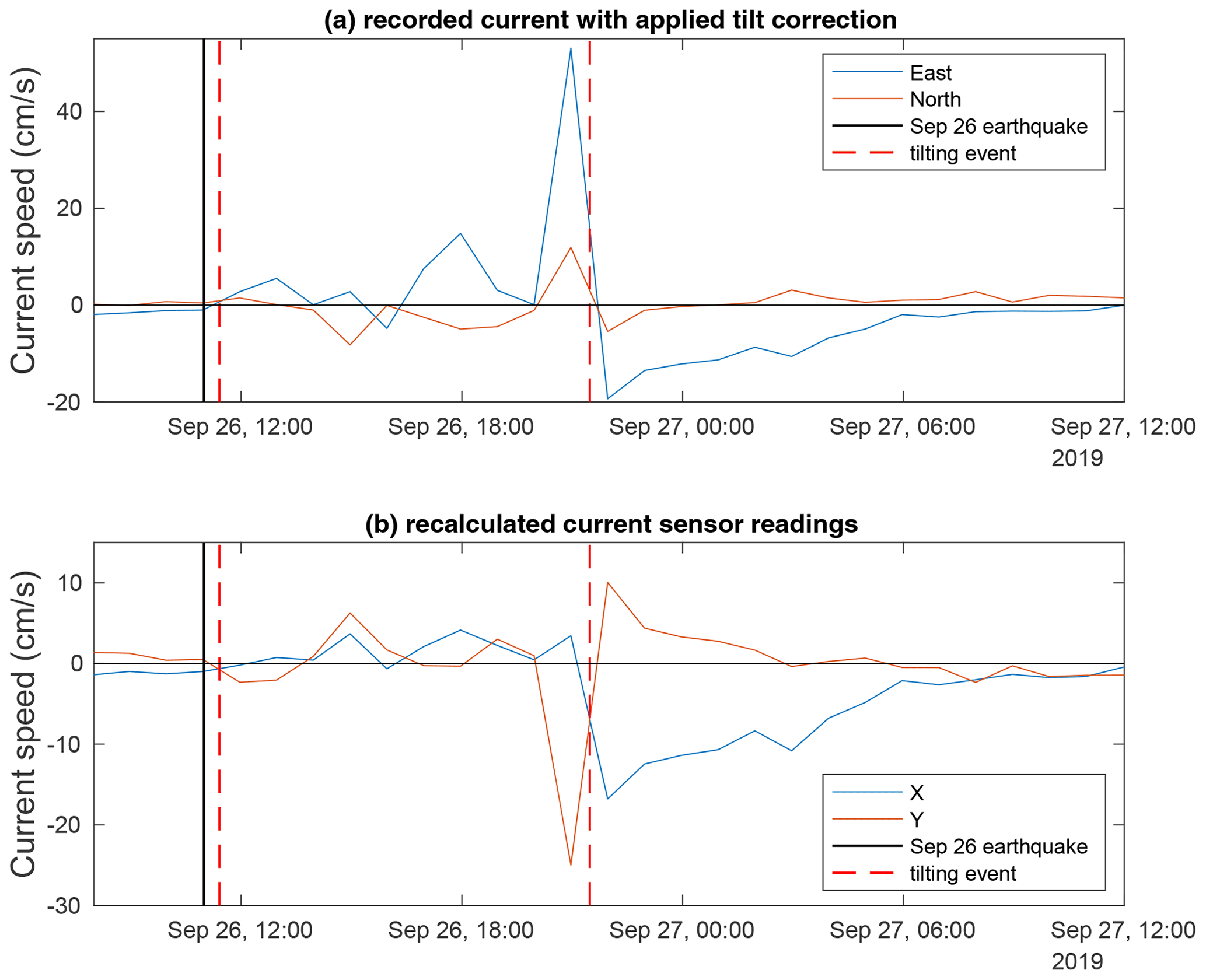
Figure 7 Current record acquired around the time of occurrence of a M_w 5.8 earthquake. (a) Instrumental record, automatically corrected for tilt and heading. (b) Recalculated readings in the x and y axis of the Doppler sensor (see text for interpretation).

After the 26 September 2019 M_w 5.8 earthquake, during the 10 h period when the instrument remained strongly tilted, the instrument recorded currents varying both in speed and orientation, but some precautions are needed when interpreting these data. The current component measured by transducers along the y axis of the instrument, oriented N 200^∘, probably remained accurate as the tilt along this axis is less than 20^∘ and the measurement cell remained above the bottom (Fig. 2b). On the other hand, the x component may not be reliable, as one of the sensors (no. 1) is oriented 65^∘ upward in the N 160^∘ direction and the opposite sensor (no. 3) is dipping 65^∘ downward in the opposite (N 340^∘) direction. Consequently, measurement cell no. 3 lies within the sediment and thus may only record noise. Moreover, because the Doppler current sensor (DCS) is set in forward pinging mode, current speed is calculated with data from sensors measuring positive Doppler shifts only. This implies that if the current component toward N 160^∘ is positive, sensor no. 1 will measure a negative shift and will not be recorded. During the time interval considered here, the measured current component in the x direction (toward N 160^∘) is positive, which indicates that data from sensor no. 3 were used (Fig. 7), and that is probably noise. It follows that the current component along the y direction is the only one reliable. The horizontal current measured along the y axis changed sign several times during this time interval and reached peak values of 6.3 cm s⁻¹ toward N 200^∘ at 14:57:46 GMT, about 4 h after the earthquake, and of 25 cm s⁻¹ in the opposite direction at 20:57:46 GMT, the last measurement before the instrument straightened up. Other measurements on both axes remain below 5 cm s⁻¹, but the absolute velocity may have been higher because this measurement was only performed in one direction. Yet, these observations suggest that the stronger current (≈25 cm s⁻¹) recorded 30 min before the instrument straightened up played a role in this event. Once the device got back into an upright position, it recorded a current consistently flowing westward and progressively decreasing from 20 cm s⁻¹ to a background level (2 cm s⁻¹) in 9 h (Fig. 4). During this waning phase, the current drift is about 3.5 km in a westward direction (Fig. 6). The drift estimated during the first 10 h after the earthquake, while the instrument was strongly tilted, is in the opposite direction but may not be reliable.

3.3 Acoustic backscatter signal

The background backscatter amplitude level is $-\mathrm{43}\pm \mathrm{1}$ dB before the earthquakes; 3–4 h after the 24 September 2019 M_w 4.7 earthquake, backscatter increases sharply to −22 dB between 11:00 and 12:00 GMT and then decays to −41 dB over 12 h. The increase in backscatter coincides with a change in current direction and speed, indicating that the turbid cloud was brought to the instrument site by the current. However, the current speed of less than 4 cm s⁻¹ may have been insufficient to put the particles in suspension. There is no increase in backscatter on 20 September when stronger currents coming from the same direction, but not related to an earthquake, were recorded.

Backscatter strength remains $-\mathrm{41}\pm \mathrm{1}$ dB for the 1.5 d interval before the 26 September 2019 M_w 5.8 earthquake and increases to the −20 to −13 dB range after the earthquake (Fig. 5). This implies sand-sized particles or flocs were put in suspension soon after the earthquake, although the local current speed remained relatively low (about 5 cm s⁻¹ at most). After the device went back to a near-vertical position, signal strength reaches a maximum of −7.6 dB, which corresponds to an amplitude ratio of 42 and an intensity ratio of 1800 compared to the base level. Similar signal strength levels are typically reached with the ZPulse sensor in highly turbid water such as in estuaries. During deep-sea deployments signal strength ranges more typically between −60 and −40 dB. After reaching a peak value, backscattered signal strength progressively decays over 3 d to stabilize at about −40 dB (Fig. 5). Several turbid events, with signal strength at about −35 dB, are observed in October and associated with small increases in current velocity (up to 3–4 cm s⁻¹). It is unclear whether these passing clouds are residual turbidity from the earthquake. After 9 October, backscatter eventually returns to its background level, while temperature decreases by 0.007 ^∘C over a few hours, indicating replacement of the water mass around the instrument.

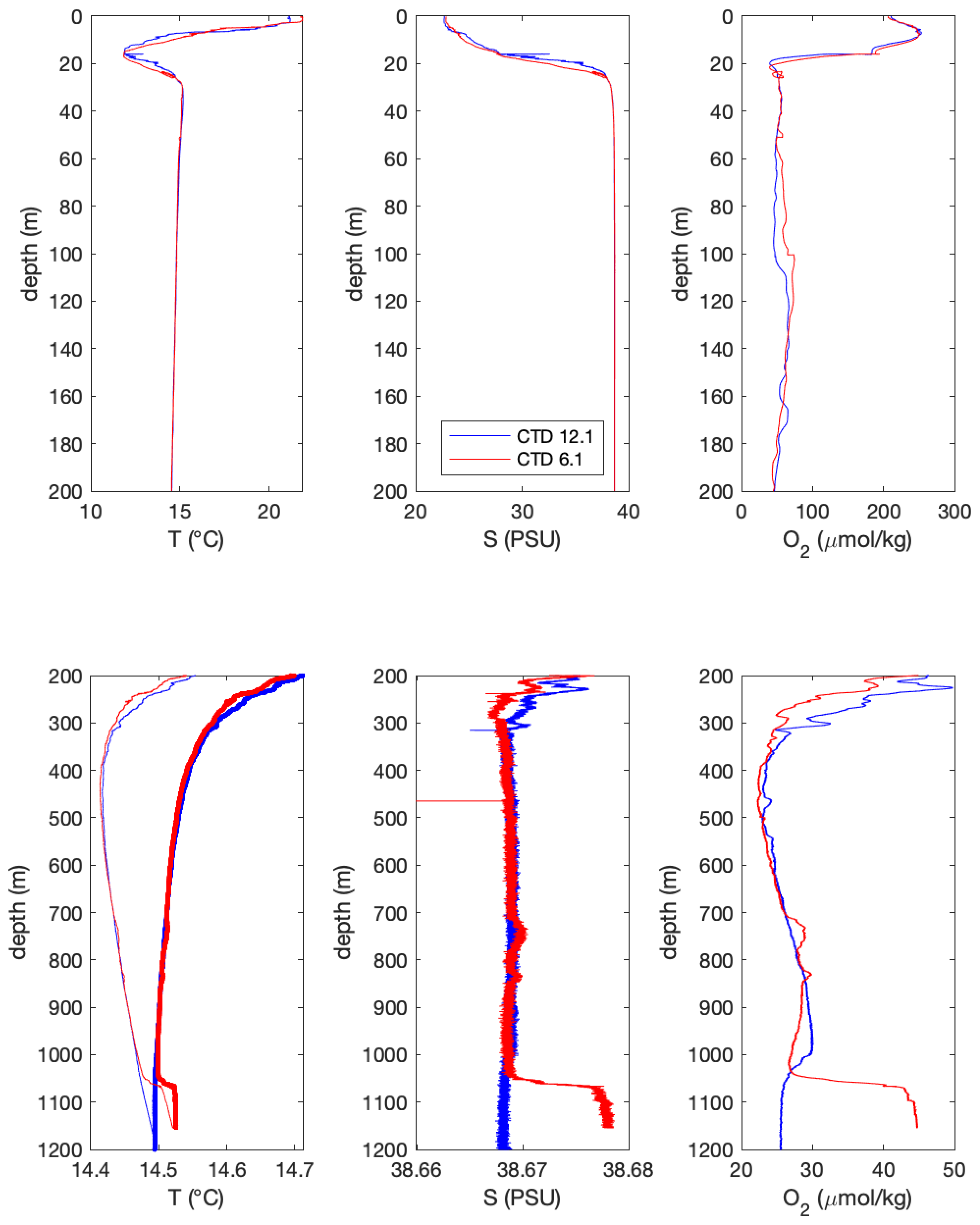
Figure 8 Depth plots of temperature (T, ^∘C), salinity (S, PSU, practical salinity unit) and oxygen concentration (O₂, µmol kg⁻¹) from CTD profiles acquired in the Sea of Marmara in June 2007 during the Marnaut cruise of Ifremer's (Institut Français de Recherche pour l'Exploitation de la Mer) R/V L'Atalante (Henry et al., 2007). On the lower temperature plot, thin lines are measured values and thick lines are conservative temperatures calculated at 1180 m. Locations are shown in Fig. 1.

3.4 Temperature record

The Sea of Marmara is stratified, with a low-salinity (20 ‰–22 ‰) 20–30 m surface layer that displays strong seasonal temperature variability (5–10 ^∘C in winter, 20–25 ^∘C in summer) overlaying a high-salinity (about 38 ‰) body of seawater at 14–15 ^∘C derived from the Aegean Sea (Beşiktepe et al., 1994). Within the high-salinity body, the conservative temperature (McDougall et al., 2013) calculated with the Gibbs SeaWater oceanographic toolbox of TEOS-10 (Thermodynamic Equation Of Seawater - 2010; McDougall and Barker, 2011) generally decreases with depth. This implies that the adiabatic temperature rise in a turbidity current, flowing downward, should cause a small temperature increase at the location of the instrument. However, the deployment site is prone to seasonal cascading within the deep waterbody so that the initial temperature structure may have been disturbed. Examples of CTD profiles recorded in June 2007 (Henry et al., 2007) are shown in Fig. 8 and indicate the presence of a slightly warmer waterbody on the seafloor, only present in the basin along the base of the slope. No CTD profile is available in September 2019, but variations in temperature and oxygen concentration associated with mild currents (<5 cm s⁻¹) were recorded by the instrument in May–July 2019 and again on 20 September. It is therefore likely that the temperature at the location of the instrument was slightly higher, by 0.01 to 0.02 ^∘C, than at the same depth in the central part of the basin.

Temperature variations associated with the 24 September 2019 M_w 4.7 earthquakes are very small, less than ±0.002 ^∘C, which confirms that water movements during this event were local. After the 26 September 2019 M_w 5.8 earthquake the recorded temperature decreases progressively by about 0.015 ^∘C to reach its minimum value when the strongest current is recorded, around the time when the instrument straightens itself (Fig. 5). After that, temperature progressively increases back to reach nearly the same value as before the event. The small variation in temperature indicates that the turbid water originates from within the deep waterbody. One remarkable observation is that temperature only starts decreasing very slowly after the tilting of the instrument. Temperature decreases at a higher rate after 14 h, which is also when the tilted instrument starts measuring significant currents.

The slight temperature decrease observed after the earthquake can result from the mixing of the warmer bottom waterbody originally present around the instrument with the bulk of the deep-water layer in the Central Basin. Moreover, the observation of a temperature drop precludes that the turbid water originates from depths less than 600 m, as water present between 600 m and the halocline is at a higher conservative temperature than the deeper water throughout the year (see Beşiktepe et al., 1994, and Fig. 8). Moreover, an inflow of water from closer to the surface should result in an increase in the O₂ concentration in the bottom water, but none is observed in the data.

4 Interpretation and discussion

4.1 Sequence of events

Let us first consider the potential influence of meteorology on the events recorded at the seafloor. Reanalyzed ERA5 hourly wind and pressure data (Hersbach et al., 2018) interpolated at the location of the instrument indicate relatively low wind (less than 5 m s⁻¹) at the time of the earthquakes and during the hydrodynamic disturbances that followed (Fig. 5). It is thus unlikely that wind influenced the course of these events. On the other hand, the current event on 20 September 2022 occurs at a time of high wind and follows a change in wind direction. Hypothetically, wind forcing may have caused this event but probably not through sediment resuspension, as acoustic backscatter remained low. A possible influence of wind on the motion of turbid clouds passing over the instrument after 2 October remains open for discussion.

The observations at the seafloor provide some insight into the complex sequence of events that followed the earthquakes and suggest the following scenarios (Table 1). After the 24 September 2019 M_w 4.7 earthquake a turbid cloud formed east of the instrument and drifted slowly. Considering the maximum velocity of the current (less than 4 cm s⁻¹) and the 4 h interval between the earthquake and the passing of the turbid cloud over the instrument, the front of turbid water should have formed east-northeast of the instrument at a maximum distance of about 500 m, and this coincides with the base of the northern slope near the outlet of the canyon. Small-scale failures on the steeper slopes on the sides of the canyon and shaking are possible causes of sediment resuspension. The clouds subsequently drifted downslope over a total horizontal distance of at most 1 km before dissipating, adding the 500 m estimate above to the drift calculated after the passing of the front over the instrument (Fig. 6).

Table 1 Event chronology. Time and magnitude of earthquakes from Karabulut et al. (2021).

The M_w 5.8 earthquake on 26 September 2019 caused stronger currents and a small temperature perturbation. Temperature records from turbidity currents invariably display a correlation between current onset and temperature change, and this temperature change is nearly always positive (Mikada et al., 2006; Palanques et al., 2008; Kasaya et al., 2009; Xu et al., 2010; Khripounoff et al., 2012; Liu et al., 2012; Hughes Clarke, 2006; Johnson et al., 2017; Brizuela et al., 2019; Normandeau et al., 2020; Heerema et al., 2022). Temperature spikes may thus be used to infer turbidity current occurrences and provenance (Johnson et al., 2017). The currents we observe are associated with a temperature decrease. Because water above 600 m water depth is at a higher potential temperature (temperature corrected for the adiabatic gradient) than water at the basin seafloor (Fig. 8), the gravity currents must come from deeper than 600 m. This rules out that they initiated at the shelf edge. Water may have been mixed locally or flowed down some distance down the slope. For instance, currents may have originated from above the earthquake rupture zone, where the seafloor lies in the 600–1200 m depth range.

The temperature records also concur with the current record to indicate that currents in the water column remained moderate for several hours after the earthquake and are not the primary cause of instrument tilting. First of all, there is a delay of at least 1 h after the earthquake (30 min after the tilting event) before temperature starts decreasing significantly. Moreover, an acceleration of the temperature rate of variation correlates with an increase in measured current speed (to about 6 cm s⁻¹) between 14:00 and 15:00 GMT (about 2 h later), indicating that the tilted current meter and the temperature sensors are providing concordant information. Even if a short burst of current may have been missed because of the 1 h interval between current records, this would not explain why the frame remained stable in a tilted position for several hours. Local liquefaction of the sediment beneath the device is also an unlikely cause because the tilting of the instrument occurred 25 min after the earthquake. A thin dense flow of remobilized sediment originating from the basin slopes thus appears as a more likely cause. Partial burial of the device is attested by presence of sandy mud caked on the device in various places: on the frame feet, on the acoustic releases, on the optode connector and also inside the plastic protection of a flotation sphere from which bindings were broken. On the other hand, the current speed of at least 25 cm s⁻¹ recorded before the time when the device straightened up is strong enough to cause erosion of mud deposits. It may thus be hypothesized that erosion freed the device from the mud cover. The flotation spheres on the frame and the concrete ballast at its base exert a moment that should keep the assembly stable in an upright position unless the frame is loaded with sediment.

Powerful turbidity currents driven by dense basal flows have notably been observed in Monterey Canyon (Paull et al., 2018) and may share some characteristics with the event reported here, although this event is much weaker. These dense flows are relatively thin (<2 m in the Monterey Canyon case) and have the ability to displace instruments before the development of turbulence in the water column. It appears likely that, after the passing of the seismic wave, failures on slopes adjacent to the deployment site caused a debris flow or dense mudflow that spread on the basin floor causing the tilting of the instrument and bottom water turbidity while turbulence in the water column remained limited. As the base of the nearest slope is about 400 m north of the instrument, this would imply a minimum velocity of 20 cm s⁻¹ for the mudflow to reach the device location in 25 min.

During the following 10 h, the current record is incomplete but indicates variations in strength and direction. One possible explanation is that widespread slope instabilities triggered by the earthquake have resulted in several turbidity currents recorded as successive pulses. Other possible explanations include oscillatory currents. However, the role of seiches and surface gravity waves can be ruled out as no tsunami was recorded by near-shore tidal gauges around the Sea of Marmara. The relationship between gravity wave amplitude A and bottom current amplitude U in the shallow-water linear approximation is given by $U=(g/H{)}^{\mathrm{1}/\mathrm{2}}A$, where H is water column height. An oscillatory current of 10 cm s⁻¹ at 1200 m depth would thus correspond to a free-surface oscillation of 1 m (or 100 hPa) for a standing wave (seiche) as well as a progressive wave (tsunami). This should have been easily detected in a sea where tidal amplitude is about 10 cm (Alpar and Yüce, 1998). The influence of baroclinic internal waves on the halocline at 20–30 m depth must also be ruled out as they cannot physically produce currents of more than a few centimeters per second at 1200 m. Nevertheless, it remains possible that the interface at the top of the turbid cloud is affected by baroclinic waves.

The strongest current is recorded after 10 h, which suggests that a turbidity current initiated further upslope (but deeper than 600 m) may have reached the site after a longer delay but may also have gained more kinetic energy on its downhill path. This event, reaching a speed exceeding 25 cm s⁻¹, apparently caused enough erosion to free the device from the mud accumulation. The current then stabilizes in a westward direction and decays progressively over the next 9 h, which suggests the tail of a turbidity current flowing in canyon E of the deployment site has been recorded. The hours-long delay between the earthquake and the passing of the fastest current over the instrument may hypothetically correspond to the time for the head of the turbidity current to travel from its source to the location of the instrument. Alternatively, a sequence of slope failures may have lasted up to several hours after the earthquake. Longer delays between loading events and turbidity currents, of several days to, possibly, months, have been observed after floods (Carter et al., 2012) or after distant earthquakes (Johnson et al., 2017). Another possibility is delayed ignition, which may occur if the turbidity current develops from the hydrodynamic instability of a dilute turbid cloud, indirectly resulting from slope failures and/or ground shaking (Parker, 1982; Mulder and Cochonnat, 1996; Piper and Normark, 2009; Hage et al., 2019). The turbidity current could thus result from multiple plumes initiated by the earthquake shaking and merging downslope.

The distance traveled by the turbidity current on the basin floor cannot be accurately estimated with a single instrumental record. However the drift plot (Fig. 6) obtained during the waning phase may be roughly indicative of the distance over which particles have been transported beyond the instrument by the turbidity current. The drift distance is 3.5 km, and, when plotted over the bathymetric map, the drift appears to stay within the depositional fan at the outlet of the canyon, the extension of which is known from sediment sounder profiles (Fig. 1). These calculations are only a rough estimate of the distance traveled by suspended particles, as only the velocity at 1.5 m above the seafloor and at a single point is known. Nevertheless, considering that the current strength will decrease with distance on the flat seafloor of the basin, it appears unlikely that sediments spread all over the 15×20 km basin floor, as this would require velocities of the order of 1 m s⁻¹, sustained over a wide area for several hours.

The decay of the backscatter signal strength over the next 3 d may reflect the settling of sand size particles, likely clay aggregates, from a dilute suspension. This decay occurs in large part after the 9 h waning phase of the turbidity current, while current velocity remains lower than 4 cm s⁻¹. For a first-order assessment, the Stokes settling velocity, an upper bound valid in dilute suspensions (e.g., Guazelli et al., 2011) may be used. The Stokes settling velocity of 63 µm quartz grains (density: 2650 kg m⁻³) in 13 ^∘C seawater is 2.7 mm s⁻¹, allowing such grains to drop by 700 m in 3 d. However, if the particles forming the cloud are mostly composed of clay aggregates, for which density may be between 1200 and 1700 kg m⁻³, the settling velocity would be between 0.3 and 1 mm s⁻¹. In this case the height of the suspended particle cloud could range between 70 and 250 m above the seafloor.

4.2 Current observations across the earthquake magnitude range

In this study a seafloor device located at the outlet of a canyon in the Central Basin in the Sea of Marmara recorded a range of turbid events and currents induced by earthquakes that has been rarely documented. In September 2019, M_w 4.7 and 5.8 earthquakes occurred at a 5 km distance from the device as well as a series of smaller foreshocks and aftershocks. In this setting, earthquakes of magnitudes less than 4 caused neither noticeable water column turbidity nor currents. The M_w 4.7 earthquake generated a turbid cloud on slopes a few hundred meters from the instrument, and the cloud took 3–4 h to drift down to the instrument location and 10 more hours to dissipate. As the current velocity remained small (less than 4 cm s⁻¹), it can be concluded that this cloud did not evolve into a self-sustained turbidity current (Parker, 1982). The M_w 5.8 earthquake initiated a turbidity current, and the data obtained may be compared with more complete records obtained elsewhere with ADCP deployments and/or water column mooring lines. A velocity of several tens of centimeters per second is representative of the slower recorded examples, corresponding to mud-rich flows associated with hyperpycnal flows or small landslides (Khripounoff et al., 2012) or to the smaller storm-related events (Normandeau et al., 2020). The event recorded is a very weak event compared to turbidity currents that followed large earthquakes or large slope instabilities. Cable breaks show that the turbidity current triggered by the 1929 Grand Banks M_s 7.2 earthquake reached velocities of at least 19 m s⁻¹ (Piper et al., 1999). Velocity of turbidity currents estimated form cable breaks in the Gaoping Canyon and Manilla Trench system range from 5.5–12.7 m s⁻¹ for the 2006 Pingtung M_L 7.0 earthquake and 5.9–7.9 m s⁻¹ for a M_L 6.4 earthquake (Gavey et al., 2017). From instrumental records, velocities of 2–7 m s⁻¹ were reported for the turbidity current following the Tohoku M_w 9.1 earthquake (Arai et al., 2013) and 1.4 m s⁻¹ in the Tokachi-Oki M_w 8.3 case (Mikada et al., 2006). The downward current after the earthquake off of Izu Peninsula may be constrained with a noisy ADCP record to a maximum of 10–15 cm s⁻¹ in a 20–30 m layer above the seafloor and lasting about 1 h, peaking about 30 min after the earthquake (Kasaya et al., 2009). This turbidity current thus appears less intense and shorter in duration than the one recorded in the Sea of Marmara, but the triggering earthquake was probably smaller (M 5.4 compared to M_w 5.8) and more distant (10 km). Moreover, the event off of Izu shares an important characteristic with the Sea of Marmara in that the turbid cloud is observed to form some time before current builds up in the water column. When the maximum velocities reported are plotted against magnitude (Fig. 9), they show a tendency for larger earthquakes to trigger stronger currents, which is hardly surprising. It also appears that estimates from cable breaks tend to give higher values than instrumental records. This may perhaps be because instruments give the maximum current speed at a single position, while cable breaks yield an integrated estimation of maximum current speed. Moreover, if cable breaks are caused by a dense basal flow, it is yet unclear how its speed relates to that of currents in the water column (Paull et al., 2018). The data set available today remains insufficient to reach general conclusions regarding scaling, and factors other than earthquake magnitude, such as slope, would need to be taken into account.

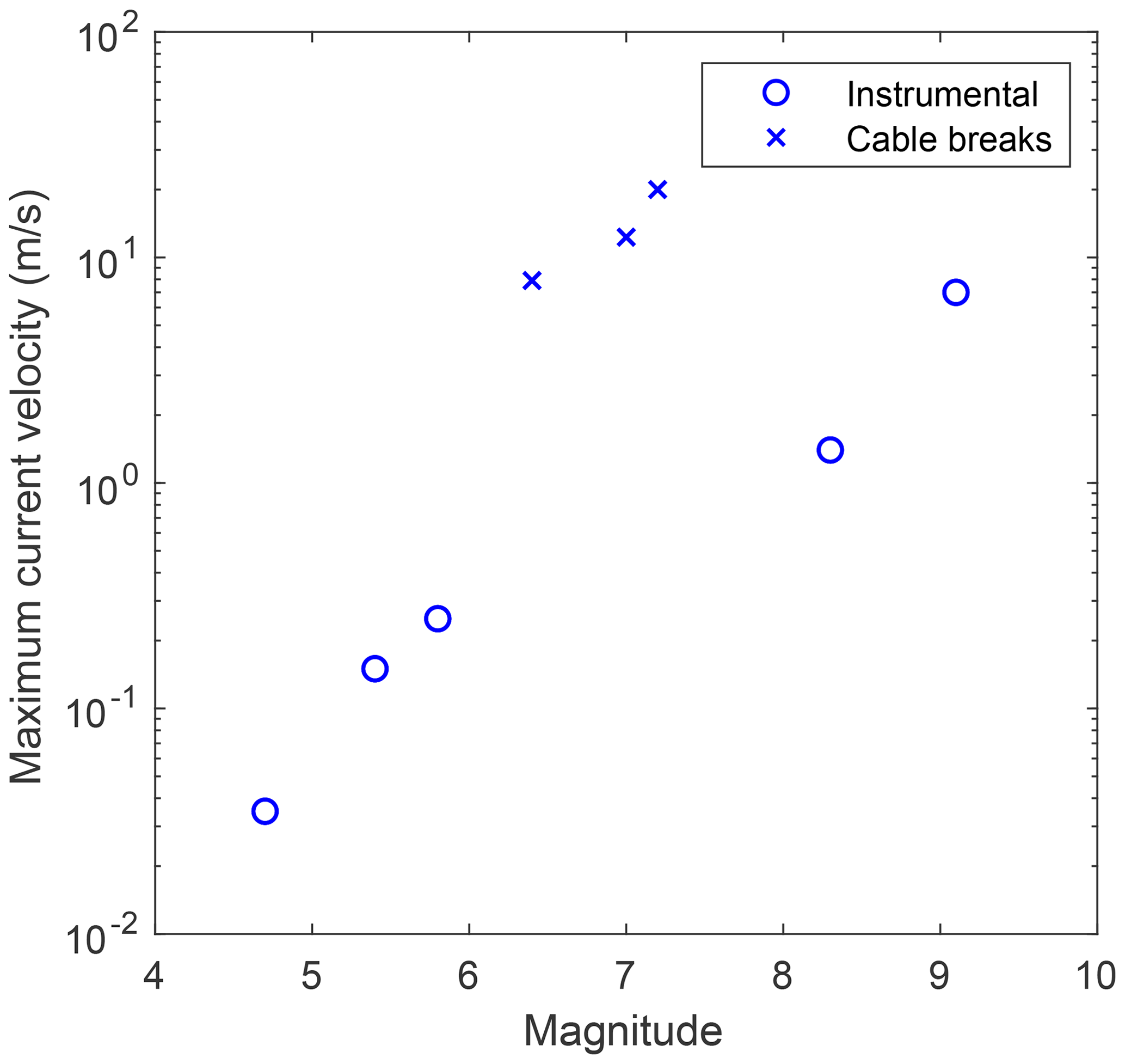
Figure 9 Maximum measured current velocity as a function of earthquake magnitude for the cases discussed in text.

4.3 Implications for sediment transport after earthquakes

Several observations from the monitoring records have special relevance for the understanding of sediment resuspension and transport processes during earthquakes. The first one is that earthquakes can induce sediment resuspension in situations where current remains too low to be the primary cause or resuspension. This is apparent when comparing events on 20 September (unrelated to an earthquake and without turbidity) and 24 September (after an M_w 4.7 earthquake and turbid) that have comparable current speeds. Resuspension may be an immediate effect of ground shaking or results from local slope failures. This process may be important as it opens the possibility of triggering turbidity currents after earthquakes by hydrodynamic instability within the water column. The second one is that a mass flow sufficiently strong and dense to displace a heavy instrument occurred at a time when there was no indication of advection in the water column. Currents in the water column apparently continued to increase in strength after this initial mass flow had stopped. A third observation is that the water displaced with the turbidity currents is deep water, as indicated by the temperature record. Likely, the displaced water originated from where the earthquake triggered sediment mobilization, which is in relatively deep water around the earthquake source area north and west of the instrument location (Fig. 1). Turbidity currents more commonly originate from continental shelf edges or the upper part of continental slopes. This is notably the case when they are related to storms, river discharge or sediment loading. However, triggering by earthquakes may affect any part of the continental slope depending on the location of active faults. The case we reported shows that a moderate earthquake (M_w 5.8) can cause sediment remobilization near the base of the slope rather than at the shelf edge, resulting in different flow dynamics than generally assumed for sediment remobilization events.

The geomorphological context of the deployment site also needs to be taken into account. It is located on a depositional fan at the outlet of a canyon and south of a slope identified as unstable from geomorphological criteria (Zitter et al., 2012). We have shown that a debris flow or dense mudflow originating from this unstable slope, followed several hours later by a turbidity current flowing along the canyon, could well explain the sequence of event following the M_w 5.8 earthquake. Although this is not the only possible explanation for the observations, we believe it is the most likely one considering the geomorphological context. We estimated that the current during this event was probably too weak to spread a layer of sediment over the entire Central Basin floor. It is also unclear whether this event left on the fan a sedimentary layer that may be identified as a seismoturbidite, as a debris flow or as a layer of homogeneous mud. Differences between the fan and the basin in the number of sedimentary events and of their characteristics could explain why the sequence of seismic reflectors on sediment sounder profiles differs in the basin and in the fan (Fig. 1). For all these reasons, the base of slope or canyon outlets are not good sampling locations for obtaining reliable earthquake records. In previous studies in the Sea of Marmara (e.g., McHugh et al., 2014), samples were taken across the basin depocenter for this purpose and events correlated between cores could also be correlated with historical earthquakes of estimated magnitude > 6.8. This approach remains in principle valid.

5 Conclusion

Instrumental records obtained in the Sea of Marmara Central Basin near the base of an unstable slope and the outlet of a canyon bring some insight into sediment remobilization by proximal (≈5 km) earthquakes and their hydrodynamic consequences.

• The smaller earthquakes (M_w<4) are not associated with water column events.

• A M_w=4.7 earthquake caused the formation of a turbid cloud and low currents not exceeding 4 cm s⁻¹.

• A M_w=5.8 earthquake at the same location caused a mass flow strong enough to capsize a heavy instrument. Subsequent movements of the water masses remained local, mixing deep waters at a scale of 5–10 km maximum.

This suggests that a continuum of hydrodynamic events of increasing intensity with earthquake magnitude occur above a threshold, corresponding to M_w≈4 at the studied location. Moderate earthquakes can thus generate mass flows and turbidity currents of limited extension that may confuse paleoseismological records in cores taken near the edges of basins. However, the local nature of these events and/or the earthquake history of the area may help distinguish them from the consequences of storms and floods expected to initiate from near the edge of the continental shelf. Performing new core studies and very high-resolution geophysical surveys in this area would thus have important implications for understanding under which conditions earthquakes leave a distinctive trace in the sediment record.