the Creative Commons Attribution 4.0 License.
the Creative Commons Attribution 4.0 License.
 | 01 Dec 2022
Comparison of machine learning techniques for reservoir outflow forecasting
José González-Cao
Diego Fernández-Nóvoa
Gonzalo Astray Dopazo
Moncho Gómez-Gesteira
Reservoirs play a key role in many human societies due to their capability to manage water resources. In addition to their role in water supply and hydropower production, their ability to retain water and control the flow makes them a valuable asset for flood mitigation. This is a key function, since extreme events have increased in the last few decades as a result of climate change, and therefore, the application of mechanisms capable of mitigating flood damage will be key in the coming decades. Having a good estimation of the outflow of a reservoir can be an advantage for water management or early warning systems. When historical data are available, data-driven models have been proven a useful tool for different hydrological applications. In this sense, this study analyzes the efficiency of different machine learning techniques to predict reservoir outflow, namely multivariate linear regression (MLR) and three artificial neural networks: multilayer perceptron (MLP), nonlinear autoregressive exogenous (NARX) and long short-term memory (LSTM). These techniques were applied to forecast the outflow of eight water reservoirs of different characteristics located in the Miño River (northwest of Spain). In general, the results obtained showed that the proposed models provided a good estimation of the outflow of the reservoirs, improving the results obtained with classical approaches such as to consider reservoir outflow equal to that of the previous day. Among the different machine learning techniques analyzed, the NARX approach was the option that provided the best estimations on average.
- Article
(5253 KB) - Full-text XML
- BibTeX
- EndNote


Humankind has been creating reservoirs since ancient times (Baba et al., 2018). The purpose of these bodies of water are varied and include irrigation, flood protection, power generation and control of the natural flow of rivers, among others (Lee et al., 2009). Reservoirs are created through the construction of dams, which are complex structures that retain water and are capable of controlling the water flow. This ability to control the flow permits the management of water resources, allowing the storage of water for consumption, electricity production and protection against floods. They are, therefore, important agents that affect the economy, human population, and fauna and flora in their area of influence (Castelletti et al., 2008). In a river basin, it is usual to find several of these structures along the course of the river; thus, the operation of the upstream reservoirs affects all the downstream activities. Therefore, communication and coordination among the different dams present in the river course are desirable for the optimal management of water resources (Marques and Tilmant, 2013; Jeuland et al., 2014; Quinn et al., 2019; Rougé et al., 2021). However, this is not always possible as there may be different barriers and trade-offs that hinder such coordination. It is not unusual for rivers to pass through different countries or administrative regions with different policies and regulations. It is also common for dams to be operated by private companies with different operating policies and interests. The operation of these structures depends not only on natural factors and well-defined operating rules but also on external demand. These aspects can also hinder access to or the utilization of the operation rules of the reservoir. This adds a significant amount of uncertainty in predicting the outflow of a reservoir at any given time, making it difficult to incorporate into physics-based models, which is a disadvantage in water resource management and flood risk prevention.
Different aspects of water reservoirs will be of increasing importance in the future. One of the most important is the key role that dams play in protection against floods, which are one of the most dangerous natural catastrophes, being the cause of tremendous loss of lives (Jonkman, 2005) and billions of euros in economic losses (Hallegatte, 2012; Wallemacq et al., 2018) worldwide. Unfortunately, several studies predict a worsening scenario for the future, increasing the frequency and severity of these phenomena (Berghuijs et al., 2017; Passerotti et al., 2020). Several factors affect this trend, with climate change (Arnell and Gosling, 2016; Liu et al., 2018) and modifications in land use (Booth and Bledsoe, 2009; Bradshaw et al., 2007; de la Paix et al., 2013; Rosburg et al., 2017), being two of the most important ones. In response to these worrying reports, the scientific community established that flood mitigation is one of the most important challenges to be addressed in the coming decades (Field et al., 2012), and dams can play a key role in this sense. In addition, in the context of climate change, hydropower generation also plays an important role. Hydropower generation is expected to increase significantly in the future in a scenario of increasing demand for renewable energies (Adaramola, 2016), although climate change may affect river flow and thus the availability of water for power generation (Berga, 2016). Issues related to water availability in future scenarios are also a major concern for such important sectors as agriculture, which negatively affect food production (Alcamo et al., 2007; Elliott et al., 2014; Xiong et al., 2009). Optimizing the management of water resources and more specifically the reservoir operations will be essential to mitigate these effects.
This research paper focuses on the development of models capable of forecasting the outflow of a reservoir. These models could be an advantage when incorporated into current or newly developed water management systems, improving their operation. This includes flood early warning systems and reservoir management systems, among others. In order to forecast the outflow of a reservoir, the most simplistic approach involves assuming that the outflow would be equal to the inflow. Although this approach is an oversimplification of river dynamics, it can be a reasonable approximation under very specific conditions, for example, in relatively small reservoirs during wet seasons when they are close to the spillway capacity after a period of high inflows and therefore have little margin to alter the natural flow of the river. Another simplistic approximation would be assuming that the outflow of the reservoir for a given day d will be the same as on day d−1. This can provide acceptable approximations under normal conditions when the flow does not vary significantly from day to day. This procedure can be improved by applying multivariate solutions that assume different weights to several known variables. In this case, the approach will be to establish a relation between the outflow on a given day d with the known outflow, inflow and reservoir level on day d−1. One approach to improve these simpler solutions is to develop data-driven models based on the analysis of the data of a specific system, being able to find relations between the input and output variables of the system. These models have been complementing or replacing physics-based models (e.g., hydrodynamic models) in the last few years (Solomatine and Ostfeld, 2008). Data-driven modeling uses machine learning (ML) techniques to build models for a specific system from existing data. According to Rashidi et al. (2019), machine learning is an application of artificial intelligence (AI) that enables the automatic learning of computer systems, all based on experience without explicit programming. Machine learning techniques have been successfully applied in many hydrological applications (Le et al., 2019; Xiang et al., 2020; Kratzert et al., 2018; Rjeily et al., 2017; Guzman et al., 2017; Lee and Tuan Resdi, 2016; Taghi Sattari et al., 2012; Ghorbani et al., 2019; Emami and Parsa, 2020; Sammen et al., 2017) in the last few years. In this paper, several methodologies based on machine learning techniques are proposed for the time series forecasting of reservoir outflow. The ML techniques used for this task are included under the category of supervised learning, meaning that the ML algorithm will be fed with data that include the desired solutions (Géron, 2019), in this case, the future outflow of a reservoir. The task to be performed by the ML model is a regression in which a target outflow value will be predicted from a series of input variables or features. This research paper will cover several techniques ranging from multivariate linear regression (MLR) to several artificial neuron network (ANN) techniques (a feed-forward neural network with a back propagation algorithm (multilayer perceptron, MLP), nonlinear autoregressive exogenous (NARX) and a long short-term memory network model (LSTM)) to forecast the outflow for different important dams located in the Miño–Sil basin (Galicia, Spain). However, it is worth noting that the results obtained in this study may not be completely extrapolated to other areas with larger reservoirs and/or dry climatic conditions. Also, it is important to clarify that the operation strategies of the dam are key to determine its outflow and they can be used in different ways to improve the prediction models. However, this research focuses on the capabilities of different machine learning approaches to forecast the total outflow of the next 24 h period and therefore infer the operation strategies from the data.
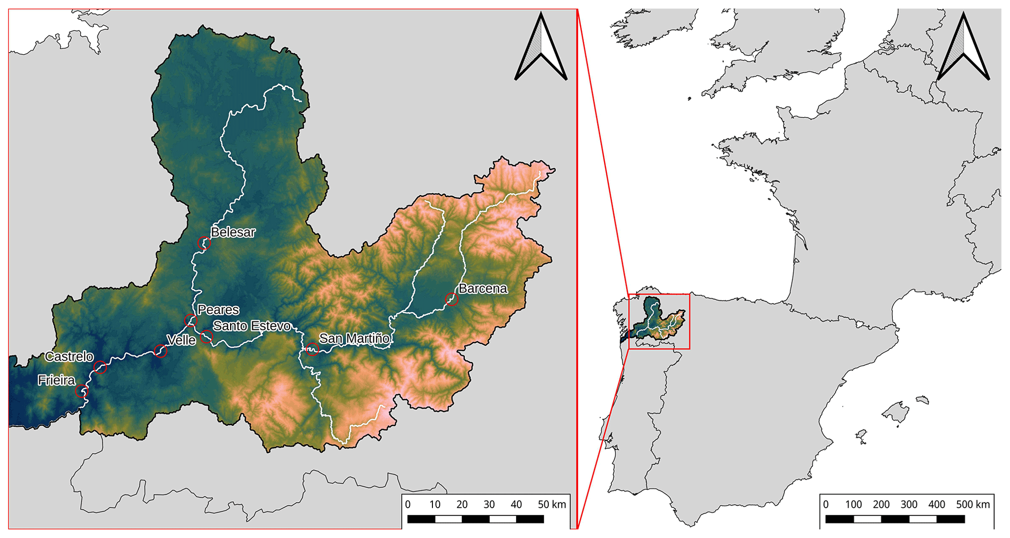
Figure 1Location of the reservoirs analyzed in this study.
The research paper is structured as follows: in Sect. 2 the characteristics of the area of study and the different ML models employed will be presented. Section 3 will analyze and discuss the results obtained. And last, in Sect. 4 the main conclusions of the study will be discussed.
2.1 Area of study
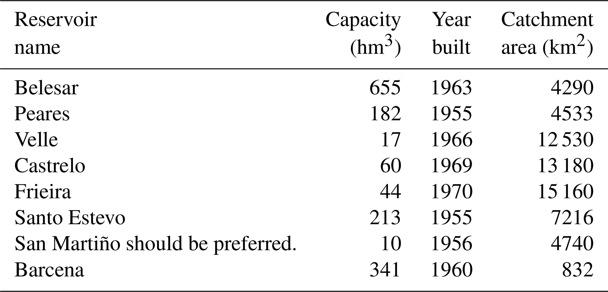
Figure 1 shows the area of study and the location of the reservoirs employed in the present work. The eight reservoirs are located in the Miño–Sil River basin, situated in the northwest of the Iberian Peninsula. The basin has a total area of around 17 000 km2 (Confederación Hidrográfica del Miño-Sil, 2016) and constitutes an important region of hydroelectric generation. The Miño–Sil River system is one of the most important in the Iberian Peninsula and has the highest runoff-to-surface ratio. It is characterized by a pluvial regime with a maximum water flow in the winter season and a minimum in summer (Fernández-Nóvoa et al., 2017), presenting average annual precipitation of 1184 mm (Confederación Hidrográfica del Miño-Sil, 2016). Eight reservoirs were selected from the Miño–Sil River system with capacities ranging from 10 to 655 hm3 (see Table 1 for a summary of their main characteristics).
Table 1List of dams analyzed in the study (data provided by Confederación Hidrográfica del Miño-Sil).
A total of 19 years of data on a daily scale were provided, after request, by the Miño-Sil River Basin Authority (Confederación Hidrográfica del Miño-Sil, https://www.chminosil.es, last access: 29 November 2022) for the reservoirs under study. The period analyzed spans from 1 October 2000 to 30 September 2019. The time series data include the percentage of filled volume, the inflow and the outflow of the reservoir.
2.2 Machine learning models
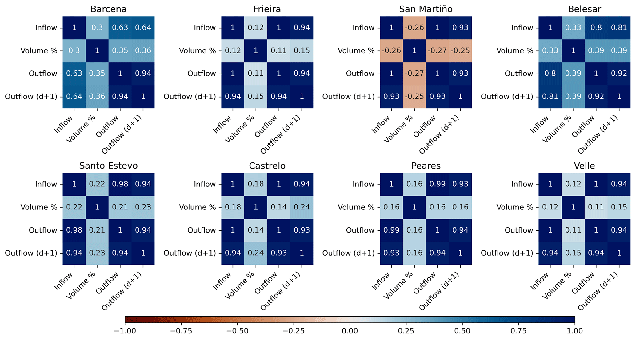
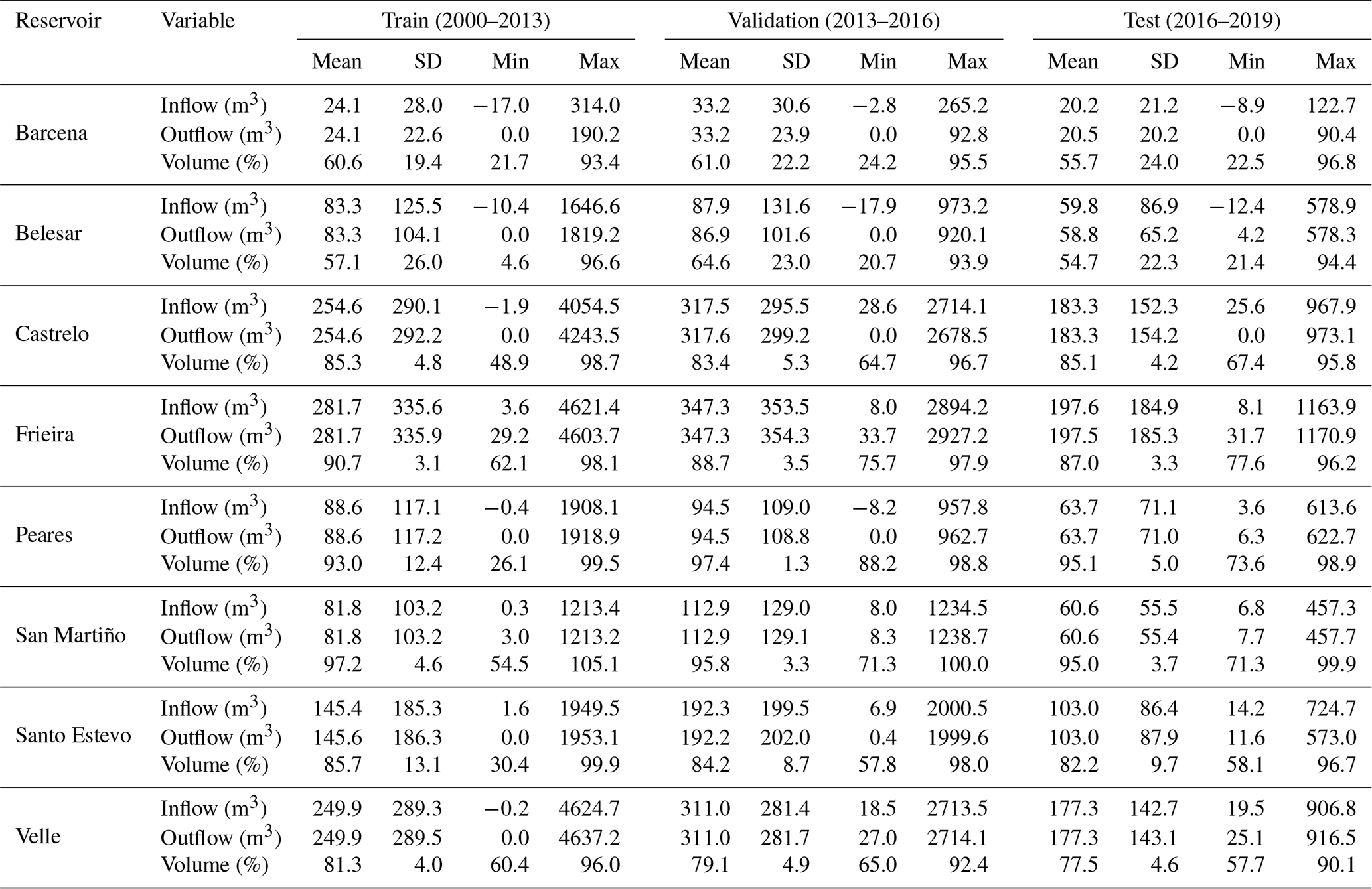
The available dataset was divided into three different subsets, using roughly the first 70 % of the data range for the training subset (from 1 October 2000 to 30 September 2013), the following 15 % for the validation subset (from 1 October 2013 to 30 September 2016) and the remaining 15 % for the test subset (from 1 October 2016 to 30 September 2019). This criterion has been chosen for better interpretation and comparison of the output series produced by the models. Table 2 shows the statistics of the subsets for each reservoir and variable. Once the training phase is completed, the unbiased model performance is tested against the test subset. This approach can help to identify overfitting problems, where a model offers good performance with the dataset used during the training phase but is not able to generalize with new input data. For all the models, the inflow, outflow and volume percent values are used as input data to predict the outflow of the next day. Figure 2 shows the correlation between the variables involved for each of the analyzed reservoirs. It can be observed that there is a strong correlation between the inflow and the outflow variables. However, the two largest reservoirs analyzed (Barcena and Belesar) show a lower correlation between inflow and outflow, which is in concordance with their higher capacity and lower average occupation. The correlation between volume percent and the outflow is low in all the cases but slightly higher in Barcena and Belesar.
Table 2Statistics of the variables used for the train, validation and test subsets.
2.2.1 Multivariate linear regression
The first ML technique based on multivariate linear regression was chosen to test complex neural network-based techniques against more conventional techniques. MLR can perform better than ANN in certain applications where the number of sample data available are small (Markham and Rakes, 1998); in this sense, this model can help to assess if the dataset available is big enough to use ANN-based models. A relation was established between the outflow and inflow measured at day d, with respect to the outflow of the next day d+1, which corresponds to the day under prediction. In addition, this adjustment was carried out not only for each dam but also for different filling levels, in order to also take into account this variable, which plays a key role in the dam's capacity to retain water. In this case, percentage sections of 10 % filling of the dam were considered, which means an adjustment when the occupied volume of the dam is less than 10 %, another when the occupied volume is between 10 %–20 % and so on.
Thus, for each dam, 10 adjustments define the outflow prediction attending to the different level of occupation, as the next equation indicates:
where is the predicted outflow for day d+1, with yd and rd being the measured outflow and inflow for day d. The three coefficients (c0, c1 and c2) were obtained from the linear fitting depending on the measured filling level of the corresponding dam.
The equation and procedure described above were applied to each dam, using in all cases the first 70 % of the data to obtain the adjustments and the last 30 % to test their efficiency. Although a validation phase is not considered in this methodology, the same dataset partitioning as in the neural network models has been used to facilitate the comparison. The first 70 % of the data (training subset) will be used to develop the model and the last 30 % to test (validation and test subsets) their efficiency. Therefore, both the validation and test subsets are both test subsets in this methodology.
2.2.2 MLP model
The second type of model developed in this research comprised ANNs, which are a type of computational approach that can be encompassed within machine learning. These types of models have been inspired by the biological human brain (Farizawani et al., 2020). An ANN model, like a biological neural network, is formed by several simple processing units joined to each other using weighted connections (Taghi Sattari et al., 2012). The simple processing unit is called a node or neuron. Artificial neural networks present different advantages over traditional approaches to model data (Livingstone et al., 1997). Perhaps and according to Livingstone et al. (1997) the most outstanding advantage is that this type of model is capable of fitting complex nonlinear models. However, according to the same authors, this type of approach also has an important disadvantage, which is that neural networks can suffer from overfitting and overtraining, but this can be solved by taking a good architecture selection and using training/control groups to see the evolution of the model (Livingstone et al., 1997).
The first type of ANN model developed in this research is an MLP ANN (multilayer perceptron artificial neural network), that is, a feed-forward neural network with a back propagation algorithm. In this type of ANN, the information moves only in a forward direction, that is, from the input neurons (in the input layer), crossing the hidden neurons (in the hidden layer) to the output neurons (RapidMiner Inc., 2022) (see Fig. 3). The back propagation algorithm is used to fit the model. This kind of supervised algorithm compares the predicted values with the real values to calculate the prediction error; then this error is fed back through the network to adjust each connection weight and reduce the prediction error in the next cycle (RapidMiner Inc., 2022); that is, these ANNs learn by adjusting the connection weights. This process continues to run until the error goes down or reaches a satisfactory level or until a previously established number of cycles has been reached (Taghi Sattari et al., 2012).

Figure 3Architecture of a multilayer perceptron with three inputs, a hidden layer with four neurons and a single output. The input variables, yd, rd and vd, are the measured outflow, inflow and volume percent for day d; meanwhile the output variable is the forecasted outflow for day d+1.
This type of artificial neural network is widely used in different predictions related to the study of water movement and dam or reservoir management. In this sense, an MLP model, with a back propagation learning algorithm, has been used to model the daily inflow into the Eleviyan reservoir (Iran) (Taghi Sattari et al., 2012). This model has been compared with a time lag recurrent neural network (TLRN) for a period between 1 September 2004 and 30 June 2007. The MLP models were developed with only one hidden layer. According to Taghi Sattari et al. (2012), both models work acceptably with low inflow values. Another interesting study where an MLP was used is in the research carried out by Ghorbani et al. (2019), who designed and evaluated a hybrid forecasting model combining a gravitational search algorithm (GSA) with an MLP to predict the water level in two lakes (Winnipesaukee and Cypress, USA). This hybrid model is compared with an MLP model that used the Levenberg–Marquardt back propagation learning algorithm and others such as hybrid models (MLP–particle swarm optimization and MLP–firefly algorithm), ARMA models and ARIMA models (Ghorbani et al., 2019). The hybrid MLP–GSA model showed a high efficacy over the other developed models and suggests, on the one hand, that it can be used in water resource management among other tasks. On the other hand, reservoir storage capacity determination is an important element in water resource management and planning, among others (Emami and Parsa, 2020). Due to this, Emami and Parsa (2020) try to predict the optimal reservoir storage capacity, using an evolutionary algorithm (inspired by imperialistic competition) along with an MLP model with a back propagation training technique, applied to Shaharchay Dam (Urmia Lake basin, Iran). According to the results, both models are satisfactory (with an RMSE of 0.041 and 0.045 for the imperialist competitive algorithm and the ANN model, respectively) (Emami and Parsa, 2020). Finally, another interesting research study is the one carried out by Sammen et al. (2017) which used a generalized regression neural network (GRNN) to predict the peak outflow in the event of a possible dam failure. Sammen et al. (2017) built six models using different dam and reservoir attributes and concluded that the GRNN model shows potential to predict peak outflow.
As previously said, the first ANN models developed were feed-forward neural networks with a back propagation algorithm. In this kind of ANN, the information passes through different layers. In the input layer, the information is received from the database, and it is sent to the hidden layer where the information is treated. Finally, this new information is sent to the output layer where a result is generated. The number of neurons in the input layer is determined by the number of input variables (inflow, outflow and volume (%) at day d) that will be used to try to predict the desired variable (outflow for day d+1). In this research, only one hidden layer was used. Finally, in the output layer, there will be as many neurons as variables to be predicted (in this case, one). The number of hidden neurons was studied between one and seven; the number of cycles was studied between 1 and 131 072 in 17 steps with a logarithmic or linear scale, and the decay parameter was used to decrease the learning rate during the learning process (true or false). The best MLP model developed (linear or logarithmic scale) was selected based on the lowest RMSE value for the validation subset.
The different MLP models were implemented in a server (AMD Ryzen 7 1800X, eight-core processor 3.60 GHz with 16 GB of RAM) located at the Department of Physical Chemistry of the University of Vigo, Campus of Ourense. The operative system used was Windows 10 Pro 20H2 with 64 bit. The MLP models were developed using RapidMiner Studio 9.8.001 software.
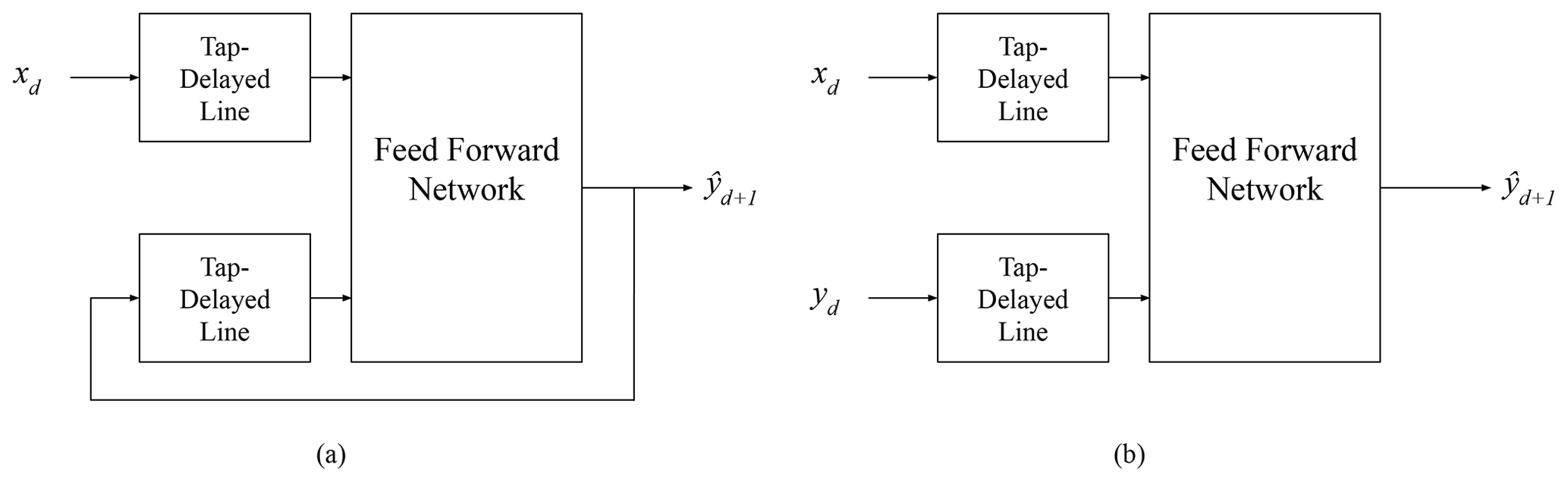
Figure 4Different architectures of a NARX model: (a) parallel architecture and (b) series-parallel architecture.
2.2.3 NARX model
The last two ANN techniques analyzed fall under the umbrella of the so-called recurrent neural networks (RNN). This kind of ANN is especially suitable to forecast time series. Nonlinear autoregressive with exogenous inputs (NARX) neural networks are a type of RNN designed for tasks with long-term dependencies on the input data. They can converge and generalize faster than other ANNs (Lin et al., 1996). NARX can use previous input and output data including a feedback delay for both input and output. There are two typical NARX model architectures: parallel (P) and series-parallel (SP) (Xie et al., 2009) (see Fig. 4). In the first one, the output of the model is fed back into the neural network, whereas in the SP architecture the real output value is used during the training phase. This second approach has proven to be more stable and robust (Amirkhani et al., 2022; Narendra and Parthasarathy, 1990). NARX models have been used in multiple hydrological applications; a NARX model was used to forecast flood risks in urban drainage systems in Rjeily et al. (2017), showing a good performance and better calculation speed compared with physically based models. Guzman et al. (2017) developed a NARX model to simulate groundwater levels in the Mississippi River valley alluvial aquifer (USA). Lee and Tuan Resdi (2016) developed a NARX model capable of making hydrological predictions at multiple gauging stations in the Kemaman catchment (Malaysia) using 13 meteorological input parameters. Yang et al. (2019) compared several RNN models including LSTM, NARX and a genetic algorithm-based NARX for reservoir operation using input data from a distributed hydrological model.
A general NARX model following the SP architecture can be expressed as
where is the predicted outflow for day d+1, yd is the measured outflow for the day d, xd denotes the exogenous input variables for day d and f is a nonlinear function that is approximated by an MLP. The parameters nx and ny refer to input and output delays. In this work, the values of nx and ny were obtained using cross-correlation functions and the value for both parameters was set equal to 5 d. The value of the number of hidden neurons was set equal to 8 by the trial-and-error method. The activation functions for the hidden layer of the neural network and the output layer are tan-sigmoid and linear, respectively. The Levenberg–Marquardt algorithm was defined to train the model using the mean square error (MSE) as the loss function. The NARX models were developed using MATLAB software (MathWorks Inc., 2022).
2.2.4 LSTM model
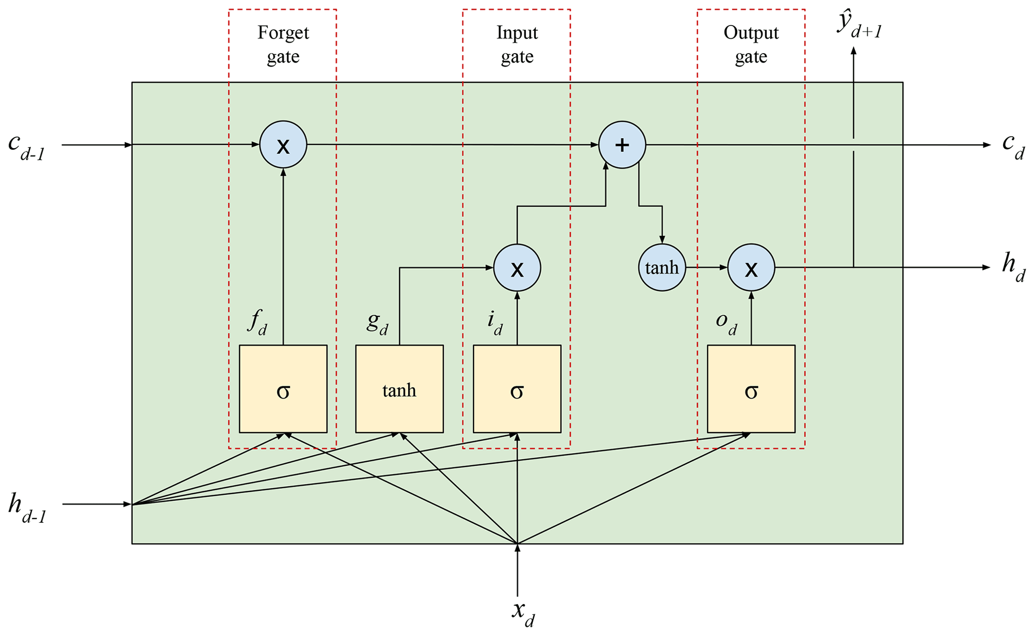
The long short-term memory (LSTM) first proposed by Hochreiter and Schmidhuber (1997) employs the so-called LSTM cell, a type of RNN memory cell that stores a short-term state hd and a long-term state cd. It is capable of identifying meaningful input data and storing them in a long-term state, keeping these data as long as necessary and using them when needed. Due to this fact, this approach is very suitable for capturing long-term patterns present in time series. As shown in Fig. 5, for each time step, as the cd−1 state enters the cell, some data are dropped in the forget gate to add some extra data coming from the input gate, resulting in cd. At the same time, a tanh function is applied to cd and passes through the output gate to produce hd, which is equivalent to . The input data xd and the short-term state hd−1 are fully connected to four layers. The main one, which outputs gd, analyzes the input and the previous short-term state as in a regular RNN, but only the most important parts are stored in the long-term state (Géron, 2019):
where tanh is the activation function, Wg is a weight matrix and bg is a bias matrix corresponding to the main layer. The remaining three layers are the gate controllers that use a sigmoidal activation function. Their outputs range from 0 to 1, and, since these outputs are used in an element-wise product, they have the ability to open or close the gate. The forget gate that outputs fd controls which part of the long-term state will be erased:
where σ is the sigmoid activation function. The input gate that outputs id controls which parts of the main layer will be added to the long-term state:
The last gate is the output gate that outputs od and controls which parts of the long-term state should be included in this time step hd and :
Therefore, the cell output and the new short- and long-term states are defined as follows:
LSTM models have been used in multiple hydrological applications. Le et al. (2019) used an LSTM neural network for flood forecasting in the Da River (Vietnam) using precipitation and the flow rate on a daily scale as input data, achieving predictions for 1, 2 and 3 d ahead showing very good Nash–Sutcliffe efficiency (NSE) values of 99 %, 95 % and 87 %, respectively. Xiang et al. (2020) used an LSTM and seq2seq (Sutskever et al., 2014) modeling approach to estimate 24 h rainfall runoff on an hourly scale in the Clear Creek and Upper Wapsipinicon River watersheds (Iowa, USA), using observed and forecasted rainfall, observed runoff, and evapotranspiration data obtained from stations. Results showed that the methodology could provide effective predictions for hydrology applications. Kratzert et al. (2018) used data from 241 catchments from the Catchment Attributes and MEteorology for Large-sample Studies (CAMELS) dataset to compare LSTM as a hydrological model versus a more traditional approach using the Sacramento Soil Moisture Accounting Model (SAC-SMA) coupled with SNOW-17, obtaining similar results with both approaches. Zhang et al. (2018) use an LSTM model to simulate the reservoir operation using 30 years of data from the Gezhouba Dam located on the Yangtze River (China), outperforming other machine learning approaches such as a back-propagating neural network and a support vector regression.
The software used for the implementation of the LSTM models was TensorFlow (TensorFlow Developers, 2022). After an exploration of different hyper-parameters, the number of hidden layers was set to one as no significant benefit was observed when using a higher number. The input width window chosen was 10 d. The input data were scaled using a standard scaler. The optimizer chosen was Adam with Nesterov momentum (Kingma and Ba, 2014; Dozat, 2016). The batch size was set to 32, obtaining similar results with values between 16 and 32 and achieving significantly worse results with higher values; these observations are in concordance with existing literature (Masters and Luschi, 2018). The activation function used is tanh, since, on the one hand, it was the only option that was optimized for graphics processing unit (GPU) accelerators, giving much faster training times but also giving more consistent results. The number of training iterations was defined by an early stopper function that stops the process when no further improvements are obtained. The cost function used during the training was the mean square error (MSE). On the other hand, the number of neurons and the learning rate parameters were optimized for each specific reservoir using the KerasTuner software (O'Malley et al., 2019).
2.3 Metrics
In order to compare the different models and measure their accuracy, several statistical metrics, widely used in hydrological applications, were employed, more precisely, Pearson's coefficient of correlation (r), the ratio of root mean square error and the standard deviation of the observed values (RSR), the NSE (Nash and Sutcliffe, 1970), and the percent bias (PBIAS) that are defined by the following equations:
where Qfor is the forecasted value, Qobs is the observed value and N is the total number of samples. Following the criterion of Moriasi et al. (2007), the statistics for model evaluation can be divided into three categories: first, the standard regression statistics that measure the linear relationship between the predictions made by a model and the observed data; in this category we considered Pearson's coefficient of correlation (r), which ranges between −1 and 1, with values close to 1 being considered to have a high degree of a positive linear relationship. The second category is the dimensionless statistics; for this case we have chosen the NSE, which ranges between −∞ and 1.0. It is a normalized statistic that computes the relative magnitude of the residual variance with respect to the variance of the observed data, with 1.0 being the optimal value. The last category is error index statistics that quantify the deviation of the predicted values compared with the observed values in the data units used. In this last category, two statistics were chosen; on the one hand, the RSR is the ratio of the RMSE to the standard deviation of the observed data, with 0 being the optimal value. On the other hand, the error index statistic used is the PBIAS, which calculates the average tendency of the predicted values to underestimate (positive PBIAS) or overestimate (negative PBIAS) the observed series.
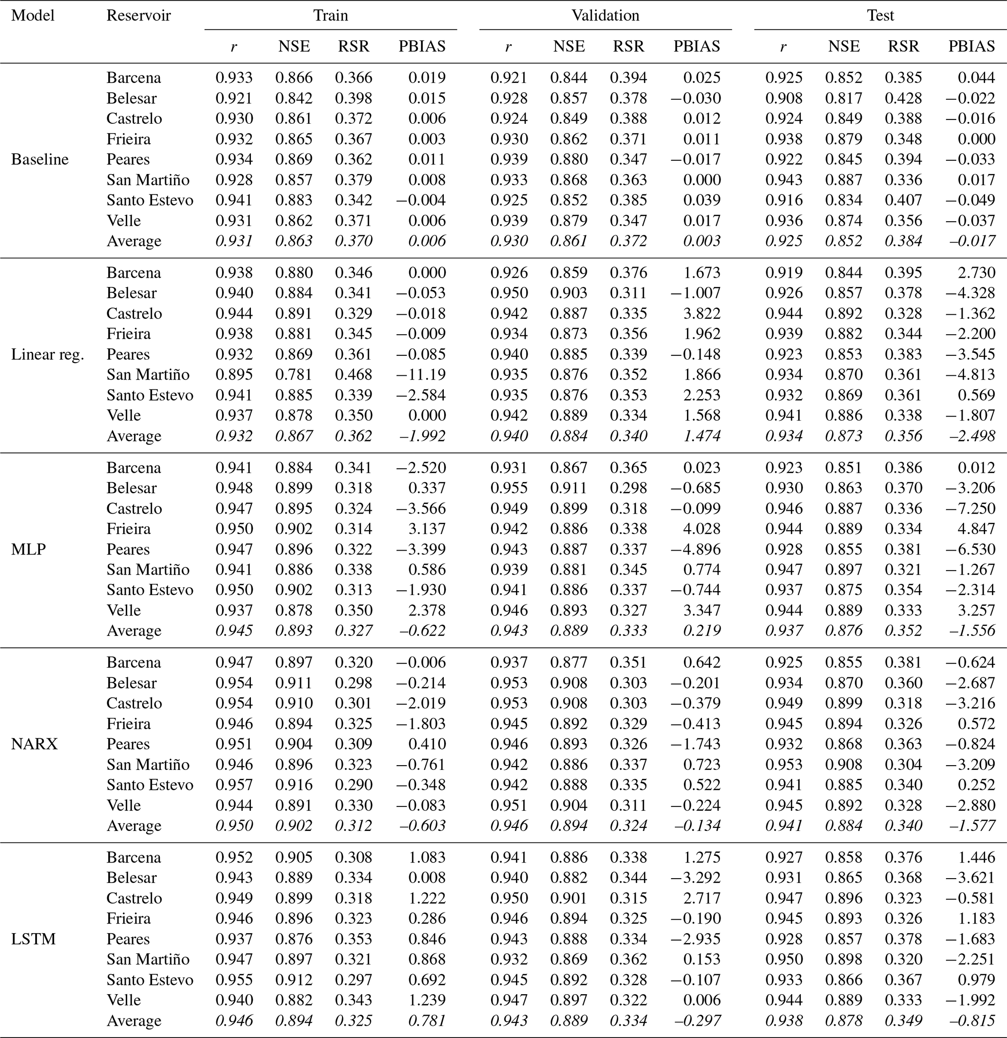
Statistical parameters used to evaluate the performance of the models to predict dam outflow are shown in Table 3. MLP models with linear scales are shown in this table due to presenting slightly better average adjustments in the validation phase than the models with logarithmic scales. Results corroborate that the proposed models offer a “very good” performance for all the subsets considered according to the criteria defined by Moriasi et al. (2007), who established different ranges of these statistical parameters to define the level of functioning of these procedures (the only exception is the PBIAS value obtained by the linear regression model in the training subset of the San Martiño reservoir). All the statistical parameters under consideration reach the maximum level of good functioning defined, and therefore it can be concluded that all the proposed models are able to provide an accurate prediction of dam outflow attending to known parameters.
The first approximation to the prediction of dam outflow was made by the simple method of considering the prediction outflow the same outflow measured on the previous day. This is considered the baseline model, to which the rest of the models will be compared. Figure 6 shows the reservoir-averaged metrics for each model and subset. As we can see in RSR, NSE and r, all the models improve the accuracy of the baseline model in every dataset. The ML model's performance shows no evidence of overfitting problems, where a trained model learns very specific features of the training dataset and fails to generalize using new datasets. The MLR approach was able to outperform the baseline model on the whole dataset but lags behind the ANN-based models. All the ANN models showed similar accuracy based on RSR, NSE and r metrics and provide a good generalization across the test subset. The LSTM models were slightly better than MLP, while NARX showed the best performance.
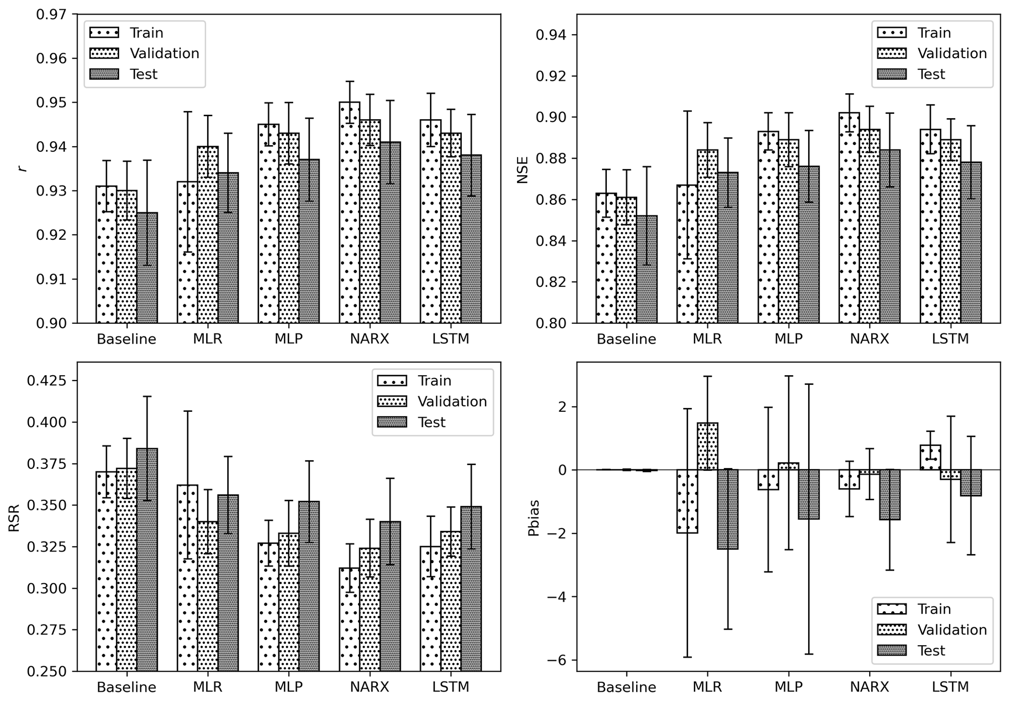
Figure 6Statistics of each subset for the different models developed. The average values from all the reservoirs are shown.
As can be observed in PBIAS (Fig. 6), the baseline does not offer any significant bias since it is the same data series as the one observed but with a delay. All the ML models have a tendency to overestimate the series, especially in the test subset. The LSTM models have the lowest tendency to overestimate and the MLR models have the highest. This fact can be very significant depending on the application of the model where a more conservative estimation towards the worst case would be preferable.
In order to analyze the differences in the performance on the different datasets and reservoirs of each model, Fig. 7 shows the NSE values for each case. Taking into account that the NSE metric is very popular among hydrology studies and no significant differences were found with RSR and r, only the NSE is shown for the sake of clarity. The MLR models provide a good generalization in Castrelo, Velle, Santo Estevo, San Martiño and Frieira reservoirs where the performance for the test dataset is very similar to or even better than on the training dataset. These are low-capacity reservoirs (excepting the Santo Estevo reservoir) where the regulation capacity is also lower. This tendency is also present in the ANN models, where the lower-capacity reservoirs (Castrelo, Velle, San Martiño and Frieira) show a better generalization ability, while in the higher-capacity reservoirs (Belesar, Barcena, Santo Estevo and Peares) the performance of the models in the test subset is lower than on the train and validation subsets. Looking more closely at the data in Table 3, a tendency is detected in reservoirs with a higher capacity to have worse statistics than those of lower capacity. This evidences that higher-capacity reservoirs have a greater ability to regulate the flow of the river according to the desired interest. In similar events, higher-capacity reservoirs have more possibilities of actuation; meanwhile lower-capacity ones have a much more limited range of options. This particularity is more difficult to be modeled by the ML models.
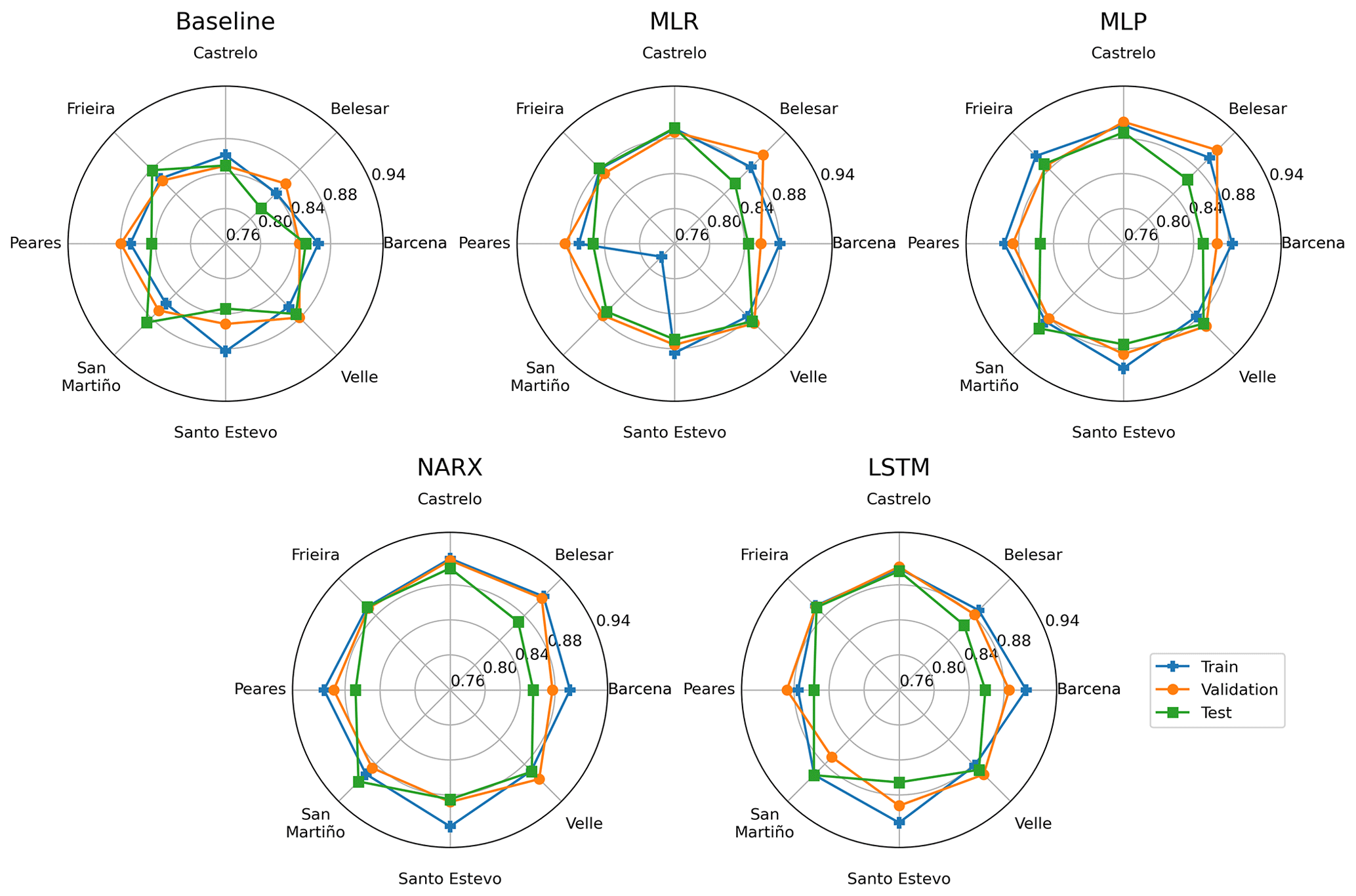
Figure 7The NSE values for each dam obtained with five methodologies for train (blue line), validation (orange line) and test (green line).
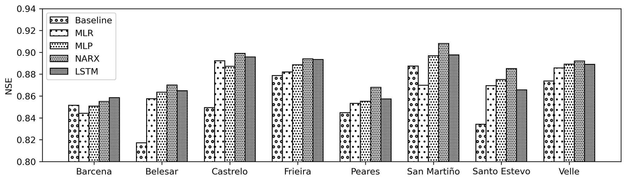
Figure 8Bar chart comparing the NSE values for the test dataset for each reservoir and model.
Table 3Statistical performance of the different models developed to predict the outflow. Averages are given in italics.
The NSE values for the test dataset for each reservoir and model are shown in Fig. 8, aiming to spot differences in the models' performance depending on the reservoir. Belesar, Castrelo and Santo Estevo reservoirs show the highest advantage for the ML models. On the contrary, in the Barcena reservoir, only NARX and LSTM were able to improve the baseline approach. The MLR models were able to outperform the baseline except in the Barcena and San Martiño cases; MLR was also able to outperform the MLP model in the Castrelo case. The MLR was never the best option but usually provides results close to ANN models. The MLP models always performed better than the baseline model except in the Barcena case; they provide similar results to the other ANN models and very close results to LSTM. The NARX models were able to improve the baseline model; they offered the best results in all the reservoirs except the Barcena reservoir, standing as the best performer. The LSTM models were also able to consistently outperform the baseline model, being the best model in the Barcena reservoir and the second best model in the rest of the reservoirs, except in Santo Estevo where it was outperformed by the MLP and NARX models. From these observations, it can be concluded that a per-reservoir analysis is advisable when developing a data-driven model, since none of the methodologies proposed can be chosen as the best for all the cases.
To illustrate the behavior of the developed models, the Belesar reservoir was chosen for two main reasons: it has the highest capacity of all the analyzed reservoirs, so it has a higher regulation capacity, and it does not have any other reservoir upstream that conditions its behavior. A comparison of the predicted and observed flow time series for the test period in the Belesar reservoir is shown in Fig. 9. It can be seen that all the methodologies show similar performance, but some differences can be highlighted. Both MLR and MLP models have underestimated the main peak of the series, while NARX and LSTM models have overestimated it. This fact should be considered when designing systems like flood EWS where the worst-case estimation should be accounted for for safety reasons. On the contrary, in the lower flows in the dry season, the NARX model was the best performer, providing accurate predictions; however, the LSTM model had some difficulties at very low flow rates, especially in the summers of 2017 and 2019. This makes the LSTM model less suitable for water management systems where the accuracy in the dry season is essential for a better exploitation of the water resources. In any case, these results may not be generalized and can differ in other scenarios.
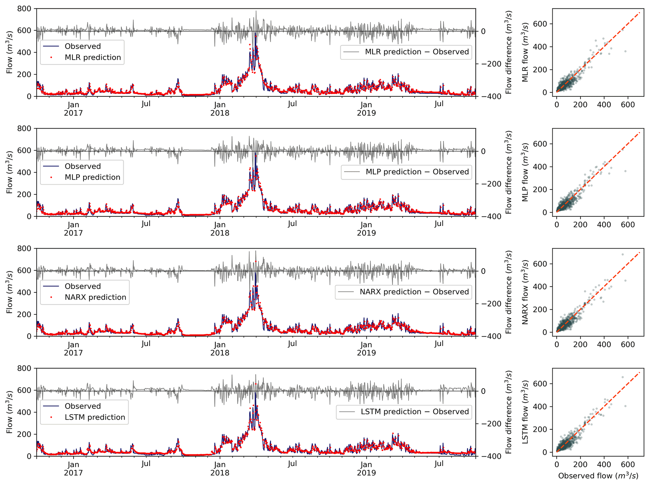
Figure 9Time series (left panels) and scatterplots (right panels) for Belesar Dam using the test dataset obtained with the proposed models.
This research paper presents an assessment of different ML techniques applied to reservoir outflow 1 d ahead prediction using the previous reservoir volume percent, inflow and outflow data. For this purpose, different models were developed and applied to several reservoirs in the Miño–Sil catchment. The analysis of the obtained results revealed that the proposed ML techniques obtained accurate predictions. The ML models provide significant improvements over the baseline model, showing a good generalization without significant signs of overfitting. On average, the MLR models were able to consistently improve the baseline model, while the ANN models provided the best results. The RNNs (NARX and LSTM) improved the MLP results, showing the advantages of the RNNs when working with time series, especially in the case of NARX. When analyzing the individual results for each reservoir, the NARX models obtained the best statistics except in the case of the Barcena reservoir, which was outperformed by the LSTM model; this evidences the need to perform a per-reservoir analysis to check the validity of each solution given the particularities of each reservoir.
The ANN is a more suitable method than MLR, given the non-linear nature of the phenomenon. Since the ANN-based models were able to outperform the more traditional MLR models, it can be concluded that the number of samples in the dataset is within the limit for training an ANN, although larger datasets would possibly lead to better models especially when dealing with extreme events.
The overall observations confirm that the analyzed ML models are capable of predicting the outflow of reservoirs and, therefore, can be incorporated into different systems such as water resource management systems or early warning systems. However, the results obtained in this research are limited to relatively small reservoirs located in wet areas and may not be extrapolated to larger reservoirs or dry areas, requiring additional research.
Although the validity of these models was assessed using only a limited range of input variables, there are many other variables that influence the functioning of the reservoirs, such as the weather forecast or the electric power demand. Also, it is possible that the addition of certain input variables like the gradient of the pool level could close the gap between MLR or MLP methodologies with recurrent neural networks. It is being studied how to incorporate these variables into these models and if they can add any improvement to the predictions.
The data are available upon request to the Confederación Hidrográfica del Miño-Sil.
All the authors of this paper participated in the conceptualization and the formal analysis of this research. OGF, JGC, DFN and GAD conducted the investigation and were involved in the development of the methodology and the software used during the study. OGF wrote the original draft of the manuscript and prepared the visualization of the results. JGC, DFN, GAD and MGG participated in reviewing and editing the manuscript. MGG supervised the research.
The contact author has declared that none of the authors has any competing interests.
Publisher's note: Copernicus Publications remains neutral with regard to jurisdictional claims in published maps and institutional affiliations.
This article is part of the special issue “Advances in machine learning for natural hazards risk assessment”. It is not associated with a conference.
We especially thank the hydrological planning office Confederación Hidrográfica Miño-Sil for providing access to historical data without which it would be impossible to conduct this study.
The aerial pictures used in this work are courtesy of the Spanish Instituto Geográfico Nacional (IGN) and part of the Plan Nacional de Ortofotografía Aérea (PNOA) program. Gonzalo Astray Dopazo also thanks RapidMiner Inc. for the different licenses of RapidMiner Studio software.
This work was partially funded by the European Regional Development Fund under the INTERREG-POCTEP project RISC_ML (code: 0034_RISC_ML_6_E). This work was also partially financed by Xunta de Galicia, Consellería de Cultura, Educación e Universidade, under Project ED431C 2021/44 Programa de Consolidación e Estructuración de Unidades de Investigación Competitivas.
Orlando García-Feal was funded by the Spanish Ministerio de Universidades and European Union – NextGenerationEU through the Margarita Salas post-doctoral grant.
Diego Fernández-Nóvoa was supported by Xunta de Galicia through a post-doctoral grant (ED481B-2021-108).
Gonzalo Astray Dopazo thanks the University of Vigo for their last contract supported by the Programa de retención de talento investigador da Universidade de Vigo para o 2018 budget application 0000 131H TAL 641.
This paper was edited by C. M. Gevaert and reviewed by three anonymous referees.
Adaramola, M.: Climate Change And The Future Of Sustainability: The Impact on Renewable Resources, CRC Press, 1–336, https://doi.org/10.1201/9781315366050, 2016.
Alcamo, J., Dronin, N., Endejan, M., Golubev, G., and Kirilenko, A.: A new assessment of climate change impacts on food production shortfalls and water availability in Russia, Global Environ. Change, 17, 429–444, https://doi.org/10.1016/j.gloenvcha.2006.12.006, 2007.
Amirkhani, S., Tootchi, A., and Chaibakhsh, A.: Fault detection and isolation of gas turbine using series–parallel NARX model, ISA Trans., 120, 205–221, https://doi.org/10.1016/j.isatra.2021.03.019, 2022.
Arnell, N. W. and Gosling, S. N.: The impacts of climate change on river flood risk at the global scale, Climatic Change, 134, 387–401, https://doi.org/10.1007/s10584-014-1084-5, 2016.
Baba, A., Tsatsanifos, C., el Gohary, F., Palerm, J., Khan, S., Mahmoudian, S. A., Ahmed, A. T., Tayfur, G., Dialynas, Y. G., and Angelakis, A. N.: Developments in water dams and water harvesting systems throughout history in different civilizations, Int. J. Hydrol., 2, 155–171, https://doi.org/10.15406/ijh.2018.02.00064, 2018.
Berga, L.: The Role of Hydropower in Climate Change Mitigation and Adaptation: A Review, Engineering, 2, 313–318, https://doi.org/10.1016/J.ENG.2016.03.004, 2016.
Berghuijs, W. R., Aalbers, E. E., Larsen, J. R., Trancoso, R., and Woods, R. A.: Recent changes in extreme floods across multiple continents, Environ. Res. Lett., 12, 114035, https://doi.org/10.1088/1748-9326/aa8847, 2017.
Booth, D. B. and Bledsoe, B. P.: Streams and urbanization, in: The Water Environment of Cities, edited by: Baker, L. A., Springer US, Boston, MA, 93–123, https://doi.org/10.1007/978-0-387-84891-4_6, 2009.
Bradshaw, C. J. A., Sodhi, N. S., Peh, K. S. H., and Brook, B. W.: Global evidence that deforestation amplifies flood risk and severity in the developing world, Global Change Biol., 13, 2379–2395, https://doi.org/10.1111/j.1365-2486.2007.01446.x, 2007.
Castelletti, A., Pianosi, F., and Soncini-Sessa, R.: Water reservoir control under economic, social and environmental constraints, Automatica, 44, 1595–1607, https://doi.org/10.1016/j.automatica.2008.03.003, 2008.
Confederación Hidrográfica del Miño-Sil: Plan hidrológico de la parte española de la Demarcación Hidrográfica del Miño-Sil, 2015–2021, https://www.chminosil.es/images/planificacion/proyecto-ph-2015-2021-vca/DOCUMENTO_DE_SINTESIS.pdf (last access: 29 November 2022), 2016.
de la Paix, M. J., Lanhai, L., Xi, C., Ahmed, S., and Varenyam, A.: Soil degradation and altered flood risk as a consequence of deforestation, Land Degrad. Dev., 24, 478–485, https://doi.org/10.1002/ldr.1147, 2013.
Dozat, T.: Incorporating Nesterov Momentum into Adam, in: ICLR Workshop, 2–4 May 2016, San Juan, Puerto Rico, 2013–2016, https://openreview.net/forum?id=OM0jvwB8jIp57ZJjtNEZ (last access: 29 November 2022), 2016.
Elliott, J., Deryng, D., Müller, C., Frieler, K., Konzmann, M., Gerten, D., Glotter, M., Flörke, M., Wada, Y., Best, N., Eisner, S., Fekete, B. M., Folberth, C., Foster, I., Gosling, S. N., Haddeland, I., Khabarov, N., Ludwig, F., Masaki, Y., Olin, S., Rosenzweig, C., Ruane, A. C., Satoh, Y., Schmid, E., Stacke, T., Tang, Q., and Wisser, D.: Constraints and potentials of future irrigation water availability on agricultural production under climate change, P. Natl. Acad. Sci. USA, 111, 3239–3244, https://doi.org/10.1073/pnas.1222474110, 2014.
Emami, S. and Parsa, J.: Comparative evaluation of imperialist competitive algorithm and artificial neural networks for estimation of reservoirs storage capacity, Appl. Water Sci., 10, 177, https://doi.org/10.1007/s13201-020-01259-3, 2020.
Farizawani, A., Puteh, M., Marina, Y., and Rivaie, A.: A review of artificial neural network learning rule based on multiple variant of conjugate gradient approaches, J. Phys.: Conf. Ser., 1529, 022–040, https://doi.org/10.1088/1742-6596/1529/2/022040, 2020.
Fernández-Nóvoa, D., deCastro, M., Des, M., Costoya, X., Mendes, R., and Gómez-Gesteira, M.: Characterization of Iberian turbid plumes by means of synoptic patterns obtained through MODIS imagery, J. Sea Res., 126, 12–25, https://doi.org/10.1016/j.seares.2017.06.013, 2017.
Field, C. B., Barros, V., Stocker, T. F., Dahe, Q., Jon Dokken, D., Ebi, K. L., Mastrandrea, M. D., Mach, K. J., Plattner, G. K., Allen, S. K., Tignor, M., and Midgley, P. M.: Managing the risks of extreme events and disasters to advance climate change adaptation: Special report of the intergovernmental panel on climate change, Cambridge University Press, 1–582, https://doi.org/10.1017/CBO9781139177245, 2012.
Géron, A.: Hands-on machine learning with Scikit-Learn, Keras and TensorFlow: concepts, tools, and techniques to build intelligent systems, O'Reilly Media, Inc., 851 pp., ISBN 9781492032649, 2019.
Ghorbani, M. A., Deo, R. C., Karimi, V., Kashani, M. H., and Ghorbani, S.: Design and implementation of a hybrid MLP-GSA model with multi-layer perceptron-gravitational search algorithm for monthly lake water level forecasting, Stoch. Environ. Res. Risk A., 33, 125–147, https://doi.org/10.1007/s00477-018-1630-1, 2019.
Guzman, S. M., Paz, J. O., and Tagert, M. L. M.: The Use of NARX Neural Networks to Forecast Daily Groundwater Levels, Water Resour. Manage., 31, 1591–1603, https://doi.org/10.1007/s11269-017-1598-5, 2017.
Hallegatte, S.: A Cost Effective Solution to Reduce Disaster Losses in Developing Countries: HydroMeteorological Services, Early Warning and Evacuation, World Bank policy research paper No. 6058, The World Bank, Washington, DC, https://doi.org/10.1596/1813-9450-6058, 2012.
Hochreiter, S. and Schmidhuber, J.: Long Short-Term Memory, Neural Comput., 9, 1735–1780, https://doi.org/10.1162/neco.1997.9.8.1735, 1997.
Jeuland, M., Baker, J., Bartlett, R., and Lacombe, G.: The costs of uncoordinated infrastructure management in multi-reservoir river basins, Environ. Res. Lett., 9, 105006, https://doi.org/10.1088/1748-9326/9/10/105006, 2014.
Jonkman, S. N.: Global perspectives on loss of human life caused by floods, Nat. Hazards, 34, 151–175, https://doi.org/10.1007/s11069-004-8891-3, 2005.
Kingma, D. P. and Ba, J.: Adam: A Method for Stochastic Optimization, ARXIV: preprint, https://doi.org/10.48550/ARXIV.1412.6980, 2014.
Kratzert, F., Klotz, D., Brenner, C., Schulz, K., and Herrnegger, M.: Rainfall-runoff modelling using Long Short-Term Memory (LSTM) networks, Hydrol. Earth Syst. Sci., 22, 6005–6022, https://doi.org/10.5194/hess-22-6005-2018, 2018.
Le, X. H., Ho, H. V., Lee, G., and Jung, S.: Application of Long Short-Term Memory (LSTM) neural network for flood forecasting, Water, 11, 1387, https://doi.org/10.3390/w11071387, 2019.
Lee, S.-Y., Hamlet, A. F., Fitzgerald, C. J., and Burges, S. J.: Optimized Flood Control in the Columbia River Basin for a Global Warming Scenario, J. Water Resour. Plan. Manage., 135, 440–450, https://doi.org/10.1061/(asce)0733-9496(2009)135:6(440), 2009.
Lee, W. K. and Tuan Resdi, T. A.: Simultaneous hydrological prediction at multiple gauging stations using the NARX network for Kemaman catchment, Terengganu, Malaysia, Hydrolog. Sci. J., 61, 2930–2945, https://doi.org/10.1080/02626667.2016.1174333, 2016.
Lin, T., Horne, B. G., Tiňo, P., and Giles, C. L.: Learning long-term dependencies in NARX recurrent neural networks, IEEE T. Neural Netw., 7, 1329–1338, https://doi.org/10.1109/72.548162, 1996.
Liu, C., Guo, L., Ye, L., Zhang, S., Zhao, Y., and Song, T.: A review of advances in China's flash flood early-warning system, Nat. Hazards, 92, 619–634, https://doi.org/10.1007/s11069-018-3173-7, 2018.
Livingstone, D. J., Manallack, D. T., and Tetko, I. v.: Data modelling with neural networks: Advantages and limitations, J. Comput.-Aid. Molec. Design, 11, 135–142, https://doi.org/10.1023/A:1008074223811, 1997.
Markham, I. S. and Rakes, T. R.: The effect of sample size and variability of data on the comparative performance of artificial neural networks and regression, Comput. Operat. Res., 25, 251–263, https://doi.org/10.1016/S0305-0548(97)00074-9, 1998.
Marques, G. F. and Tilmant, A.: The economic value of coordination in large-scale multireservoir systems: The Parana River case, Water Resour. Res., 49, 7546–7557, https://doi.org/10.1002/2013WR013679, 2013.
Masters, D. and Luschi, C.: Revisiting Small Batch Training for Deep Neural Networks, ARXIV: preprint, https://doi.org/10.48550/ARXIV.1804.07612, 2018.
MathWorks Inc.: Design Time Series NARX Feedback Neural Networks – MATLAB & Simulink, https://es.mathworks.com/help/deeplearning/ug/design-time-series-narx-feedback-neural-networks.html, last access: 29 November 2022.
Moriasi, D. N., Arnold, J. G., van Liew, M. W., Bingner, R. L., Harmel, R. D., and Veith, T. L.: Model Evaluation Guidelines for Systematic Quantification of Accuracy in Watershed Simulations, T. ASABE, 50, 885–900, https://doi.org/10.13031/2013.23153, 2007.
Narendra, K. S. and Parthasarathy, K.: Identification and Control of Dynamical Systems Using Neural Networks, IEEE T. Neural Netw., 1, 4–27, https://doi.org/10.1109/72.80202, 1990.
Nash, J. E. and Sutcliffe, J. V.: River flow forecasting through conceptual models part I – A discussion of principles, J. Hydrol., 10, 282–290, https://doi.org/10.1016/0022-1694(70)90255-6, 1970.
O'Malley, T., Bursztein, E., Long, J., Chollet, F., Jin, H., Invernizzi, L., and others: KerasTuner, GitHub [software], https://github.com/keras-team/keras-tuner (last access: 29 November 2022), 2019.
Passerotti, G., Massazza, G., Pezzoli, A., Bigi, V., Zsótér, E., and Rosso, M.: Hydrological model application in the Sirba river: Early warning system and GloFAS improvements, Water, 12, 620, https://doi.org/10.3390/w12030620, 2020.
Quinn, J. D., Reed, P. M., Giuliani, M., and Castelletti, A.: What Is Controlling Our Control Rules? Opening the Black Box of Multireservoir Operating Policies Using Time-Varying Sensitivity Analysis, Water Resour. Res., 55, 5962–5984, https://doi.org/10.1029/2018WR024177, 2019.
RapidMiner Inc.: Neural Net – RapidMiner Documentation, https://docs.rapidminer.com/latest/studio/operators/modeling/predictive/neural_nets/neural_net.html, last access: 29 November 2022.
Rashidi, H. H., Tran, N. K., Betts, E. V., Howell, L. P., and Green, R.: Artificial Intelligence and Machine Learning in Pathology: The Present Landscape of Supervised Methods, Academic Pathol., 6, 2374289519873088, https://doi.org/10.1177/2374289519873088, 2019.
Rjeily, Y. A., Abbas, O., Sadek, M., Shahrour, I., and Chehade, F. H.: Flood forecasting within urban drainage systems using NARX neural network, Water Sci. Technol., 76, 2401–2412, https://doi.org/10.2166/wst.2017.409, 2017.
Rosburg, T. T., Nelson, P. A., and Bledsoe, B. P.: Effects of Urbanization on Flow Duration and Stream Flashiness: A Case Study of Puget Sound Streams, Western Washington, USA, J. Am. Water Resour. Assoc., 53, 493–507, https://doi.org/10.1111/1752-1688.12511, 2017.
Rougé, C., Reed, P. M., Grogan, D. S., Zuidema, S., Prusevich, A., Glidden, S., Lamontagne, J. R., and Lammers, R. B.: Coordination and control-limits in standard representations of multi-reservoir operations in hydrological modeling, Hydrol. Earth Syst. Sci., 25, 1365–1388, https://doi.org/10.5194/hess-25-1365-2021, 2021.
Sammen, S. S., Mohamed, T. A., Ghazali, A. H., El-Shafie, A. H., and Sidek, L. M.: Generalized Regression Neural Network for Prediction of Peak Outflow from Dam Breach, Water Resour. Manage., 31, 549–562, https://doi.org/10.1007/s11269-016-1547-8, 2017.
Solomatine, D. P. and Ostfeld, A.: Data-driven modelling: Some past experiences and new approaches, J. Hydroinform., 10, 3–22, https://doi.org/10.2166/hydro.2008.015, 2008.
Sutskever, I., Vinyals, O., and Le, Q. V.: Sequence to Sequence Learning with Neural Networks, in: Advances in Neural Information Processing Systems, Curran Associates, Inc., ISBN 9781510800410, https://proceedings.neurips.cc/paper/2014/file/a14ac55a4f27472c5d894ec1c3c743d2-Paper.pdf (last access: 29 November 2022), 2014.
Taghi Sattari, M., Yurekli, K., and Pal, M.: Performance evaluation of artificial neural network approaches in forecasting reservoir inflow, Appl. Math. Model., 36, 2649–2657, https://doi.org/10.1016/j.apm.2011.09.048, 2012.
TensorFlow Developers: TensorFlow, Zenodo [software], https://doi.org/10.5281/ZENODO.4724125, 2022.
Wallemacq, P., House, R., Below, R., and McLean, D.: Economic losses, poverty & disasters: 1998–2017, Brussels, Belgium, https://www.undrr.org/publication/economic-losses-poverty-disasters-1998-2017 (last access: 29 November 2022) 2018.
Xiang, Z., Yan, J., and Demir, I.: A Rainfall-Runoff Model With LSTM-Based Sequence-to-Sequence Learning, Water Resour. Res., 56, e2019WR02532, https://doi.org/10.1029/2019WR025326, 2020.
Xie, H., Tang, H., and Liao, Y. H.: Time series prediction based on narx neural networks: An advanced approach, in: Proceedings of the 2009 International Conference on Machine Learning and Cybernetics, 12–15 July 2009, Baoding, Hebei, China, 1275–1279, https://doi.org/10.1109/ICMLC.2009.5212326, 2009.
Xiong, W., Conway, D., Lin, E., Xu, Y., Ju, H., Jiang, J., Holman, I., and Li, Y.: Future cereal production in China: The interaction of climate change, water availability and socio-economic scenarios, Global Environ. Change, 19, 34–44, https://doi.org/10.1016/j.gloenvcha.2008.10.006, 2009.
Yang, S., Yang, D., Chen, J., and Zhao, B.: Real-time reservoir operation using recurrent neural networks and inflow forecast from a distributed hydrological model, J. Hydrol., 579, 124229, https://doi.org/10.1016/j.jhydrol.2019.124229, 2019.
Zhang, D., Lin, J., Peng, Q., Wang, D., Yang, T., Sorooshian, S., Liu, X., and Zhuang, J.: Modeling and simulating of reservoir operation using the artificial neural network, support vector regression, deep learning algorithm, J. Hydrol., 565, 720–736, https://doi.org/10.1016/j.jhydrol.2018.08.050, 2018.