the Creative Commons Attribution 4.0 License.
the Creative Commons Attribution 4.0 License.
 | 15 Nov 2022
Timing landslide and flash flood events from SAR satellite: a regionally applicable methodology illustrated in African cloud-covered tropical environments
Axel A. J. Deijns
Olivier Dewitte
Wim Thiery
Nicolas d'Oreye
Jean-Philippe Malet
François Kervyn
Landslides and flash floods are geomorphic hazards (GHs) that often co-occur and interact. They generally occur very quickly, leading to catastrophic socioeconomic impacts. Understanding the temporal patterns of occurrence of GH events is essential for hazard assessment, early warning, and disaster risk reduction strategies. However, temporal information is often poorly constrained, especially in frequently cloud-covered tropical regions, where optical-based satellite data are insufficient. Here we present a regionally applicable methodology to accurately estimate GH event timing that requires no prior knowledge of the GH event timing, using synthetic aperture radar (SAR) remote sensing. SAR can penetrate through clouds and therefore provides an ideal tool for constraining GH event timing. We use the open-access Copernicus Sentinel-1 (S1) SAR satellite that provides global coverage, high spatial resolution (∼10–15 m), and a high repeat time (6–12 d) from 2016 to 2020. We investigate the amplitude, detrended amplitude, spatial amplitude correlation, coherence, and detrended coherence time series in their suitability to constrain GH event timing. We apply the methodology on four recent large GH events located in Uganda, Rwanda, Burundi, and the Democratic Republic of the Congo (DRC) containing a total of about 2500 manually mapped landslides and flash flood features located in several contrasting landscape types. The amplitude and detrended amplitude time series in our methodology do not prove to be effective in accurate GH event timing estimation, with estimated timing accuracies ranging from a 13 to 1000 d difference. A clear increase in accuracy is obtained from spatial amplitude correlation (SAC) with estimated timing accuracies ranging from a 1 to 85 d difference. However, the most accurate results are achieved with coherence and detrended coherence with estimated timing accuracies ranging from a 1 to 47 d difference. The amplitude time series reflect the influence of seasonal dynamics, which cause the timing estimations to be further away from the actual GH event occurrence compared to the other data products. Timing estimations are generally closer to the actual GH event occurrence for GH events within homogenous densely vegetated landscape and further for GH events within complex cultivated heterogenous landscapes. We believe that the complexity of the different contrasting landscapes we study is an added value for the transferability of the methodology, and together with the open-access and global coverage of S1 data it has the potential to be widely applicable.
- Article
(7657 KB) - Full-text XML
- BibTeX
- EndNote


Landslides and flash floods are geomorphic hazards (GHs) that can occur very quickly, sometimes in a matter of a few hours. GHs frequently co-occur and interact (e.g. Rengers et al., 2016); they have a significant impact on the landscape (Petersen, 2001; Korup et al., 2010) and are severe threats for infrastructure and human life (Bradshaw et al., 2007; Kjekstad and Highland, 2009; Froude and Petley, 2018). Landslides and flash floods are often studied in isolation. However, it is their combined occurrence that can lead to more extreme impacts. For example, in 2013, several people were killed and ∼7000 lost their homes in the Rwenzori Mountains in Uganda by a single debris-rich flash flood fed by upstream landslides (Jacobs et al., 2016a). Also, in 2011, a combination of flash flooding and mudslides across the highlands of the state of Rio de Janeiro claimed the lives of 916 people and left 35 000 people homeless (Marengo and Alves, 2012).
Understanding the temporal occurrence of GH events is essential for hazard assessment, early warning, and disaster risk reduction strategies (van Westen et al., 2008; Ali et al., 2017; Liu et al., 2018; Guzzetti et al., 2020). Temporal information with an accuracy of a few days is needed to understand the close association between precipitation and the occurrence of GH events (Guzzetti et al., 2008, 2020; Turkington et al., 2014; Marc et al., 2018). For site-specific and local-scale investigation, this accurate information on the timing of GH events can be obtained with field-based approaches such as watershed/hillslope monitoring (Guzzetti et al., 2012) or a network of observers (Jacobs et al., 2019; Sekajugo et al., 2022). However, when information on the timing of GH events is needed at a regional level, the acquisition of such data can only be achieved with satellite remote sensing (Joyce et al., 2009; Le Cozannet et al., 2020), especially in mountainous regions with difficult field accessibility and where monitoring and observation capacities are limited (Dewitte et al., 2021).
Satellite remote sensing, and more specifically the use of optical imagery, is a well-developed field of research to accurately determine the location of GH (Stumpf et al., 2014; Behling et al., 2014, 2016; Mohan et al., 2021). Optical-based satellite approaches can also be used for extracting the information on the timing of the GH events (e.g. Kennedy et al., 2018; Deijns et al., 2020); however such approaches are of limited use in cloud-covered environments, especially if temporal information with an accuracy of a few days is needed.
Synthetic aperture radar (SAR) satellite, which is an active system with the ability to penetrate cloud cover, holds a great potential for characterising the timing of GHs. Additionally, the sensitivity of SAR satellite data to surface changes, including vegetation changes (Hagberg et al., 1995; Balzter, 2001; Barrett et al., 2012), soil moisture changes (Dobson and Ulaby, 1986; Dubois et al., 1995; Ulaby et al., 1996; Nolan and Fatland, 2003; Srivastava et al., 2006), and surface texture changes (Dzurisin, 2006) gives SAR the potential to display GH timing with an accuracy of days.
SAR-derived products typically used for GH (event) analysis are amplitude data (i.e. changes in surface backscattering intensity of SAR signal between two images) (e.g. Mondini, 2017; Mondini et al., 2019; Esposito et al., 2020; DeVries et al., 2020; Handwerger et al., 2022) for which amplitude correlation is a common method used in amplitude change detection (Mondini et al., 2017; Konishi and Suga, 2018; Jung and Yun, 2020) and the coherence (i.e. the change in the ability of SAR wave fronts to stay spatially and/or temporally in phase between the two images of an interferometric pair) (Burrows et al., 2019, 2020; Tzouvaras et al., 2020). Additionally, there is a wide range of studies that use SAR-derived ground deformation to map landslides (Casagli et al., 2017; Solari et al., 2020) or analyse pre-cursor movements (Intrieri et al., 2018) and internal variability (Nobile et al., 2018). However, they are dependent on consistent high coherence values at the GH locations, which will make these methods of limited use in highly vegetated landscapes (e.g. the tropics) (Komac et al., 2015; Solari et al., 2020) and for fast-moving GHs (e.g. shallow landslides and flash floods) (Burrows et al., 2020; Tzouvaras et al., 2020). In recent GH detection studies, amplitude products are usually preferred over coherence products (Ge et al., 2019; Jung and Yun, 2020; Mondini et al., 2021), since coherence generally yields less accurate results due to lower resolution (Burrows et al., 2019, 2020) and a higher number of false positives (Aimaiti et al., 2019; Jung and Yun, 2020). Despite the increasing use of SAR imagery for GH detection (Martinis et al., 2015; Psomiadis, 2016; Twele et al., 2016; Mondini et al., 2019; Burrows et al., 2020; Jung and Yun, 2020; Tzouvaras et al., 2020; Jacquemart and Tiampo, 2021; Handwerger et al., 2022), to date, only the recent study of Burrows et al. (2022) used SAR to refine the timing of GH inventories. Although located in the tropics and showing accurate results, their study was only applied (1) within a relatively densely vegetated landscape, (2) only on landslides, (3) using pre-processed amplitude imagery with Google Earth Engine (GEE) (Gorelick et al., 2017) and (4) with a priori knowledge on the timing of the event (i.e. the year). GH events occur within a variety of landscapes (Emberson et al., 2020; Dewitte et al., 2021). Therefore, there is a clear need to calibrate and validate any GH timing method for varying landscape, and land use/land cover characteristics. Additionally, the frequent co-occurrence of landslides and flash floods (Jacobs et al., 2016b; Rengers et al., 2016) warrants the need to analyse them using a combined methodology. However, so far, there has never been research dedicated to their combined temporal detection using radar satellite.
The Copernicus Sentinel-1 (S1) constellation is frequently used in GH detection studies (Mondini et al., 2021). Next to the fact that it is freely available and acquired regionally (from 2016 onwards), it offers a very good trade-off between frequency of acquisition ( d) and spatial resolution (10–15 m depending on the pre-processing parameters). These advantages make S1 an attractive tool to integrate in a regional GH timing methodology.
In this study, we aim to develop a regionally applicable methodology that automatically estimates GH event timing using S1 SAR imagery on GH events spatially located, but with unspecified timing. We analyse landslides and flash floods together as being co-occurring and interacting events. We create a methodology that can be applied at the regional scale in complex and various topographic and land use/land cover environments. The methodology is developed using four GH events containing either landslides or a combination of landslides and flash floods located in contrasting landscape types observed within tropical Africa (see Sect. 2.1). We analyse an unprecedented number of S1 SAR products, namely amplitude, spatial amplitude correlation (a metric based on the common amplitude correlation), and coherence. Specifically, we (1) create S1 SAR time series and analyse their patterns and behaviour at the location of several GH events, (2) demonstrate and assess the ability to detect the timing of GH events using changes within the S1 SAR time series, and (3) investigate the influences of the landscape characteristics on the ability to derive the timing from S1 SAR time series through a sensitivity analysis.
2.1 Selection of GH events in a tropical region with diverse landscapes
We focus on the western branch of the East African Rift, a mountainous region with high population densities and diverse landscape and land use/land cover characteristics (Depicker et al., 2021; Dewitte et al., 2021). The region has a bimodal precipitation distribution with two rainy peaks (October–November and March–April) and a main dry season (June–August) associated with the north–south migration of the Intertropical Convergence Zone (ITCZ) (Thiery et al., 2015; Nicholson, 2017; Monsieurs et al., 2018a) with annual precipitation ranging from ∼0.8 m along the shores of Lake Tanganyika to easily more than 2 m in the highlands, with the maximum in the Rwenzori Mountains (Monsieurs, 2020; Van de Walle et al., 2020). The seasonality of the precipitation strongly controls the occurrence of landslides and flash floods (Jacobs et al., 2016a, b; Monsieurs et al., 2018a, b; Kubwimana et al., 2021). Vegetation dynamics are high in the cultivated areas due to the variety of cropping practices (crop rotations and shifting cultivation, Heri-Kazi and Bielders, 2021). Moreover, the region is one of the most cloud-covered places in the world (Robinson et al., 2019) and a global hotspot of thunderstorm activity (Thiery et al., 2016, 2017; Peterson et al., 2021).
We investigate four GH events with known days of occurrence and located in contrasting landscapes (Fig. 1):
-
Event 1 (Uganda GH event) is located in the southern part of the Rwenzori Mountains (Uganda) and counts 1063 landslide features of which some contribute directly to the sediment load of the valley river (Fig. 1, Uganda). The event occurred between 21 and 22 May 2020. The terrain consists of pristine forests and some cultivated landscape (Fig. 2a).
-
Event 2 (Rwanda GH event) is located in the Karongi District (Western Province, Rwanda), counts 494 features composed of both landslide and flash floods, and occurred on 6 May 2018 (Fig. 1, Rwanda). The terrain consists of an inhabited and highly cultivated landscape with the presence of agricultural terraces (Fig. 2b).
-
Event 3 (Burundi GH event) occurred around the hills of Nyempundu in the Cibitoke region (north Burundi), counts 318 features composed of landslides and flash floods, and occurred between 4 and 5 December 2019. Here, many landslides contribute directly to the sediment load of the rivers (Fig. 1, Burundi). The terrain consists of inhabited cultivated landscape and sporadic tree cover (Fig. 2c).
-
Event 4 (Democratic Republic of the Congo GH event) occurred west of the city of Uvira (DRC), northwest of Lake Tanganyika, and counts 609 landslides and flash flood features that occurred between 16 and 17 April 2020. Many landslides are connected to the rivers where the flash floods occurred. The debris-rich flash floods inundated parts of the city (Fig. 1, DRC). The terrain is characterised by an urban area, cultivated landscape, grassland, and sporadic tree cover (Fig. 2d).
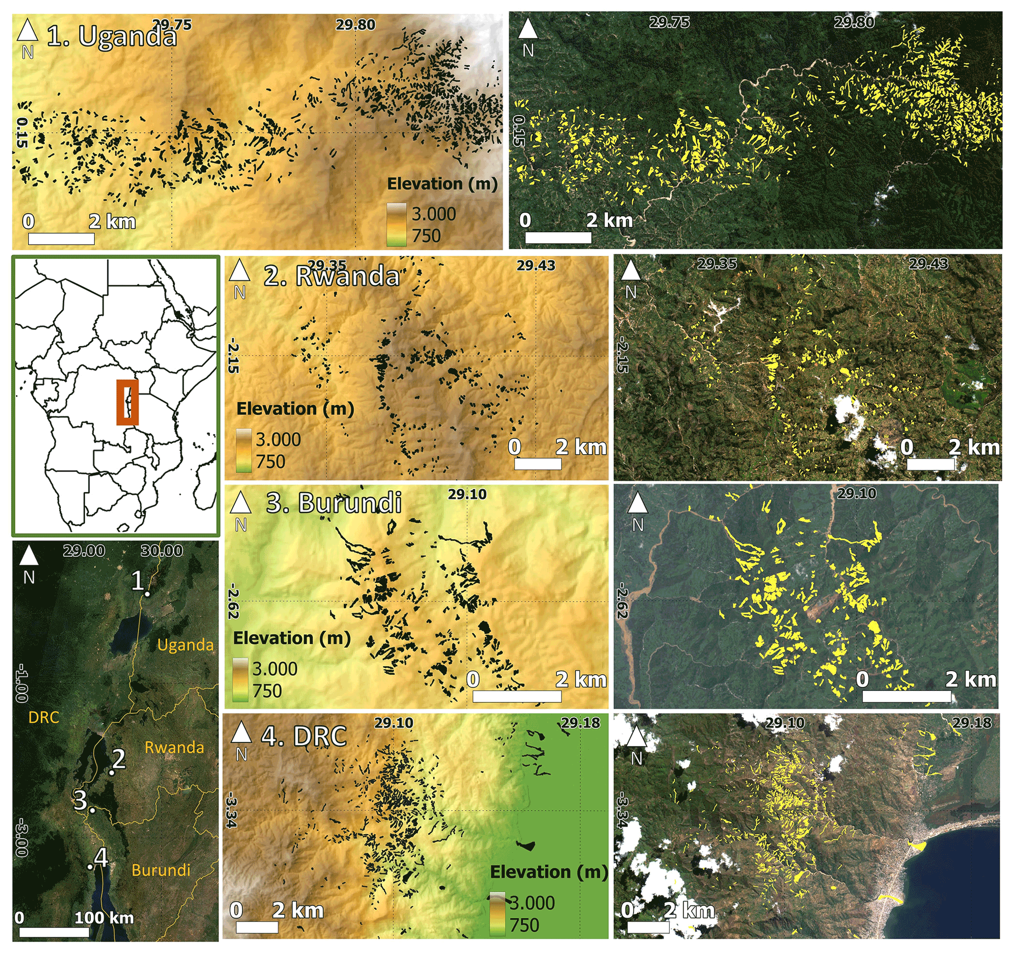
Figure 1The location of the four GH events with their topographic (left: 30 m ALOS 3D digital elevation model (DEM), GH event features in black) and optical (right: S2 post-event image, GH event features in yellow) context. Note that in the close vicinity of the GH events of Uganda and Burundi, large sediment-loaded riverbeds are visible. This is a consequence of the GH events that contributed directly to the transport of extra material to the rivers, increasing not only their sediment content but also their lateral mobility. These river dynamics are not included in our analysis. The two panels at the lower left depict the location of the GH sites (S2 imagery). Image credit: contains modified Copernicus Sentinel data (2022), processed with Google Earth Engine. ALOS 3D DEM data provided by Japan Aerospace Exploration Agency (JAXA).

Figure 2Closeup of the contrasting typical landscapes of the four GH events. Maps data: Google, © 2022 CNES/Airbus (a, b), Google, © 2022 Maxar Technologies (c, d).
The locations of the GH events (Fig. 1) are derived using the Copernicus Sentinel-2 (S2) Multispectral Instrument (MSI), high-resolution (10 m), high-frequency (6–12 d) satellite imagery. We manually digitised all individual features from the first available cloud-free S2 image after the event and a cloud-free S2 image with similar vegetation characteristics (compared to the post-event image) before the event. We use PlanetScope Ortho Scenes (Planet Team, 2017) for validation of the GH event inventory with a higher-resolution satellite image. Planet operates with a constellation of multiple small satellites producing very high-resolution (3 m), high-frequency (up to 1 d) imagery (Table 1).
Table 1Image information of manual mapping and dating GH events. Planet images are of the type PlanetScope Ortho Scene (POS).

We prefer the use of Planet and S2 over the Maxar or the Spot/Pléiades images visible in Google Earth because of the consistency in temporal and spatial resolution. To note, the Burundi GH event has recently been mapped by Emberson et al. (2022) by means of a semi-automated method followed by a manual correction using S2 satellite data. We expect our manually mapped Burundi GH event inventory to be similar or more accurate since we use a combination of S2 and Planet satellite data and a completely manual detection workflow. The date of GH event occurrences is determined from local media and field observations, and if not available from these resources it is determined by the first and last available imagery from S2 and Planet imagery.
2.2 SAR time series
SAR time series at the GH location are constructed using the Copernicus S1 Level-1 Single Look Complex (SLC) imagery acquired in Interferometric Wide (IW) swath. The S1 satellite is side-looking (right) and operates both on the ascending (from south to north) and descending (from north to south) tracks within the C-band frequency. To study the four GH events (Fig. 1) we use all available high-resolution S1 imagery ( m resolution) from January 2016 to January 2021 at the location of the GH event at tracks 174 (ascending) and 21 (descending). This equals between 196 and 208 ascending and 120 and 193 descending images per GH event, where images occasionally overlap more than one GH event with a repeat time of 6 to 12 d with more consistently 6 d towards recent times. We use both amplitude and coherence information. S1 images over the study area are provided in vertical–vertical (VV) and vertical–horizontal (VH) polarisations. Different polarisations result in different backscattering values (Shibayama et al., 2015; Psomiadis, 2016; Park and Lee, 2019; Burrows et al., 2022). Mondini et al. (2019) noted a better definition of landslide-induced changes in vegetated areas using the VH channel. In contrast, Burrows et al. (2022) found VV to perform better than VH for landslide event timing estimation. Psomiadis (2016) concluded that VV polarisation performed better than VH polarisation for flash flood mapping. Finally, VV polarisation images are acquired more consistently at the locations of our GH events. We therefore decide to use VV polarisation for our analysis. Due to the side-looking nature of the S1 satellite, it is subjected to foreshortening, layover, and shadowing, which are SAR-inherent quality problems that are amplified within mountainous regions and affect image quality (Hanssen, 2001; Dzurisin, 2006). GH inventories are masked for foreshortening, layover, and shadow areas to remove the individual landslides and flash floods that fall within these inherently noisy areas.
2.3 SAR controlling factors
SAR amplitude and coherence are influenced by local slope angle (Hanssen, 2001), soil moisture (Ulaby et al., 1996; Scott et al., 2017), vegetation (Balzter, 2001; Barrett et al., 2012), and terrain roughness (Dzurisin, 2006). Coherence is additionally influenced by atmospheric changes (Rocca et al., 2000) and due to the use of image pairs, also by the temporal baseline (time between acquisition of two images), the perpendicular baseline (distance between the location of acquisition of two images), and the difference in incident angle of the paired images (Hanssen, 2001). Coherence values are generally very low (high decorrelation) in densely forested areas due to constant movement of the leaves and stems (Weydahl, 2001; Tessari et al., 2017), whereas bare soils or urbanised terrains, due to their static nature, generally reveal relatively high coherence values (Colesanti and Wasowski, 2006). An increase in coherence values after GH event occurrence is therefore expected. Amplitude values, on the other hand, show to have a quite complex reaction to terrain change. Due to the influence of soil moisture and roughness change on the amplitude values, the occurrence of a GH event could both increase and decrease the amplitude values at the location of the GH event (Mondini et al., 2021; Burrows et al., 2022). Both precipitation (in changing leaf and soil wetness) and vegetation patterns can dynamically influence SAR amplitude and coherence values, causing a cumulative effect on the time series (Srivastava et al., 2006; Brancato et al., 2017). This effect is more prominent over sparsely vegetated areas due to geometric (vegetation growth and farming practices) and dielectric (moisture) changes (Strozzi et al., 2000). Additionally, a change in atmosphere (precipitation events, ionospheric disturbances) can dynamically influence the coherence values (Rocca et al., 2000; Jacquemart and Tiampo, 2021). To better assess the ability to detect GH timing, it is essential to understand the dynamic factors controlling the behaviour of the signal.
We derive precipitation estimates from the Global Precipitation Measurement (GPM) Level 3 Integrated Multi-satellite Retrievals for GPM (IMERG) final daily (10 km spatial resolution) dataset that has been validated through rain gauge data within the area (Nakulopa et al. 2022). General vegetation patterns per GH event are visualised using the normalised difference vegetation index (NDVI; Tucker, 1979). NDVI time series are derived from the Landsat 8 (30 m spatial resolution) archive and processed within the GEE environment. We use the Landsat 8 atmospherically corrected surface reflectance images provided within the GEE environment. We masked them for clouds using the quality assessment band resulting from the C Function of Mask (CFMask) algorithm (Foga et al., 2017).
We choose the lower-resolution Landsat 8 over the higher-resolution S2 imagery to reduce any unwanted local effects of NDVI change captured in the higher resolution S2 imagery, and since we are only interested in the general vegetation trends within the area this should be sufficient. From the cloud-masked images, a spatial-average NDVI time series is created spanning from 2016–2020 over the undisturbed areas of the GH event area. The NDVI time series are further processed to monthly averages, since we are interested in general vegetation patterns visible in the NDVI time series rather than changes on smaller temporal timescales.
We use the ESA Climate Change Initiative Land Cover product (ESA, 2016) to categorise GH based on their prior land cover to assess the influence of land cover on the timing detectability. This product has been validated within the region by Depicker et al. (2021), showing an accuracy of 86.1±2.1 % in land cover classification. All abovementioned factors are considered during the analysis of the SAR time series and the GH event timing estimations.
3.1 Sentinel-1 pre-processing
The S1 images are pre-processed using the “InSAR automated Mass processing Toolbox for Multidimensional time series” (MasTer) (Derauw et al., 2020; d'Oreye et al., 2021) processing chain (Fig. 3, step 1). MasTer is a tool for automated SAR and SAR interferometry (InSAR) mass processing (Samsonov and d'Oreye, 2012; Derauw et al., 2019, 2020; d'Oreye et al., 2019, 2021) that is incremental (i.e. only computes the minimal required information when a new image is available) and optimised for mass processing. The MasTer workflow is applied on both the ascending and descending track and consists of the following:
-
The application of orbit correction using the precise orbit files provided with the S1 data.
-
The creation of time series of amplitude maps per track. Amplitude maps of each given track are co-registered on a reference image taken from that track. Every amplitude image in the radar geometry of that track is cropped and provided with the same grid and dimensions framing the area of interest. Amplitude values are calibrated to sigma nought values. The amplitude images are multi-looked by a factor 2 in azimuth and in range, to reduce speckle, leading to a roughly 28×5 m slant range resolution. Radiometric terrain correction is applied to account for the local incidence angle variating with slope angle resulting in amplitude values that are independent of slope angle (Small, 2011).
-
The creation of time series of coherence maps per track. Coherence maps are created using consecutive images throughout the time series for each track with a maximum temporal baseline of 12 d and a maximum perpendicular baseline of 150 m. The coherence maps are provided with the same multi-looking factor, grid, and ground range resolution as the amplitude images.
-
Geocoding the amplitude and coherence maps. The amplitude and coherence from all the tracks spanning a given GH area are geocoded from slant range to ground range on a common grid with a 15 m by 15 m resolution using the 30 m ALOS Global Digital Surface Model. We decided to geocode the SAR imagery to make it compatible with all our other data products and to allow for an easier visual comparison with optical imagery.
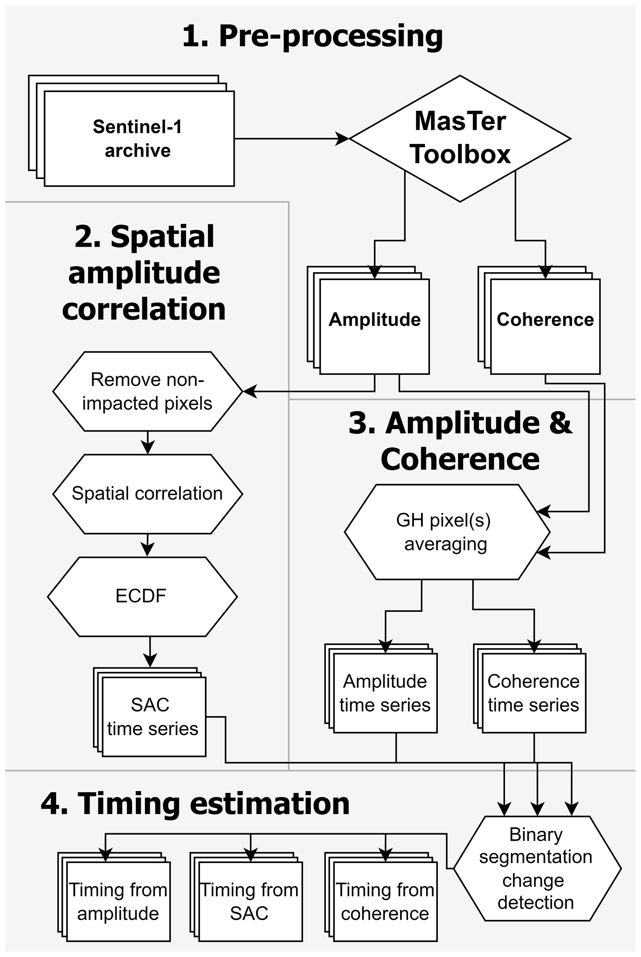
Figure 3Flowchart of the four-step methodology. Rectangles represent initial input imagery, output image stacks, or time series products. The rhombus represents the external software product. Hexagons represent methodological steps, which are described in the text. (1) Pre-processing of the S1 imagery using the MasTer processing chain to acquire amplitude and coherence image stacks. (2) Application of the spatial amplitude correlation (SAC) method using empirical cumulative distribution functions (ECDFs) on the amplitude image stack resulting into SAC time series. (3) GH pixel(s) averaging for every image in the amplitude and coherence image stacks resulting in amplitude and coherence time series. (4) Application of binary segmentation change detection to acquire the date of the most significant change within the amplitude, SAC, and coherence time series.
3.2 Spatial amplitude correlation
We adapt the amplitude correlation approach, initially used for GH spatial detection (Mondini, 2017; Konishi and Suga, 2018; Jung and Yun, 2020), to allow for GH timing detection at the location of the GH event using the amplitude image stacks (Fig. 3, step 2). We reason that the spatial correlation is generally lost when the inter-pixel relationships between two images change at the location of a GH event. Therefore, a significant change within the landscape such as a landslide or a flash flood will cause a significant decorrelation. Due to the sensitivity of SAR amplitude to changes in vegetation (Balzter, 2001; Barrett et al., 2012), seasonal greening and browning trends have a pronounced influence on the amplitude time series (Balzter, 2001; Barrett et al., 2012), which potentially limits the detectability of the GH event within the time series. Since spatial correlation is only changing when the inter-pixel relationships change, general trends that affect the entire area (lowering or increasing the SAR amplitude values) do not influence the inter-pixel relationships (i.e. no spatial correlation change). Only when significant inter-pixel change occurs, due to landslides or flash floods, will the spatial correlation change. The spatial amplitude correlation (SAC) can therefore highlight the GH event occurrence within the time series, while reducing the seasonal dynamics. To calculate the SAC, we use Eq. (1) that we adapted from Jung and Yun (2020).
with SAC the spatial amplitude correlation for the impacted area of date x in reference to date r, Ax,poly the amplitude pixels of impacted area at date x, and Ar,poly the amplitude pixels of impacted area at reference date r. Instead of calculating correlation between two subsequent images over a given window, we calculate the correlation using one reference image (Ar) and all the other images within the time series (Ax) using only the pixels within a designated impacted area (e.g. single GH feature or complete GH event) (subscript “poly”). Consequently, every image within the amplitude image stack can be used as a reference image, and due to slight changes within every amplitude image this will inevitably result in different SAC time series, one better highlighting the GH event than the other. We apply the equation separately for ascending and descending images in a parallel workflow. Figure 4 shows schematically how the SAC time series should behave using different reference images. Taking a reference amplitude image before the GH event occurrence (Fig. 4a) results in high SAC before and low SAC after GH event occurrence. The opposite is expected when using a reference amplitude image after the GH event (Fig. 4b).
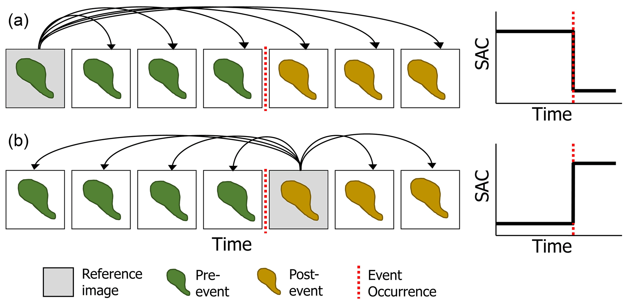
Figure 4Idealised schematic of the SAC method using two different reference images: one before and one after the occurrence of the GH event (a, b). Squares represent images; the red dotted line indicates the occurrence of a GH event. Inside the images are the conditions of the impacted area (represented here as single GH feature but similar for complete GH event). Pre-event conditions are displayed in green. Post-event conditions are displayed in brown. The black curved lines represent the combination of images on which Eq. (1) is applied to achieve the resulting SAC time series. The schematic SAC graphs (right) depict the expected results using a reference image before the event (a) with high correlation before and low correlation after the event and using a reference image after the event (b) with low correlation before and high correlation after the event.
We use every available image within the amplitude image stack as a reference image and calculated the respective SAC time series from it. From here, it is necessary to identify the most appropriate reference image.
Hence, we develop a new methodology that identifies the most suitable reference amplitude image by finding the SAC time series that most distinctively shows changes related to the GH event occurrence. We distribute every SAC time series as empirical cumulative distribution functions (ECDFs) resulting in multiple ECDF curves equal to the number of reference images. A SAC time series that contains a distinct change indicative of the GH event occurrence will show a similar distinct change in its ECDF. Contrastingly, SAC time series that fail to distinctively highlight the GH event show an ECDF that is similar to a normally distributed ECDF. Therefore, we create a normally distributed ECDF, using the mean and standard deviation derived from the ensemble of ECDF curves, and identify the ECDF that deviates most from it. Per ECDF we calculate and cumulate the difference from the normally distributed ECDF. The ECDF with the highest cumulative difference is chosen as most representative, and the related SAC time series was used.
3.3 Geomorphic hazard event timing estimation
GH event timing is determined on two scales within separate workflows:
-
Timing workflow 1: the complete GH event scale. In this workflow, the steps outlined in Fig. 3 are carried out once using all pixels encompassing the full GH event. This results in one ascending and one descending track time series for amplitude, SAC, and coherence.
-
Timing workflow 2: the individual GH scale. In this workflow, the GH event is subdivided in multiple individual GH features and the steps outlined in Fig. 3 are carried out separately for each individual GH feature. This results in multiple ascending and multiple descending track time series, equal to the number of individual GH features, for amplitude, SAC, and coherence.
In both workflows, we do not choose to remove fuzzy pixels (i.e. edge pixels that contain both impacted and non-impacted landscape) since we do not know the effect of these pixels on the SAR time series and GH event timing estimations. This allows us to establish baseline results. The ascending and descending track data are processed separately throughout the two workflows. Amplitude and coherence time series are generated by averaging the values within the identified impacted area per image (Fig. 3, step 3), and the SAC time series are generated by applying the SAC method (Fig. 3, step 2; Sect. 3.2) within both workflows. The resulting time series are normalised using the time series average to improve comparability.
Additionally, we make an effort to remove the seasonal influence and atmospheric effect on the amplitude and coherence time series by subtracting the regional amplitude and coherence trend (i.e. time series) from the GH event scale amplitude and coherence time series (timing workflow 1). Both precipitation events and seasonal vegetation dynamics are expected to cover the complete GH event and its surrounding area. This detrending will therefore emphasise the change induced by the GH event occurrence while removing any regional changes induced by either seasonal vegetation dynamics or atmospheric effects (e.g. Jacquemart and Tiampo, 2021). The regional amplitude and coherence time series are established by following step 1 and 3 in the methodology flowchart (Fig. 3), using a larger area surrounding the GH events as input (i.e. a square of approx. 1.5 times the GH event area, excluding the exact location of the GH event). This results in the detrended amplitude and detrended coherence data products. SAC is created to already consider seasonal vegetation dynamics, so no additional detrending for this data product is performed.
We decide not to detrend individual GH feature time series (timing workflow 2), which could include the use of a detrending buffer (e.g. Burrows et al., 2022). Since we deal with complex heterogenous land cover, proximate land cover does not necessarily represent the land cover at the GH feature, which prohibits it from accurately detrending. Additional research is required before implementing such a method within a wide variety of environments.
Timing is defined on every time series (for amplitude, SAC, and coherence) using a binary segmentation change detection approach (Bai, 1997; Fryzlewicz, 2014) using the Python package ”ruptures” (Truong et al., 2020) (Fig. 3, Step 4). The algorithm was set to predict only one breakpoint since we aim to detect the most significant change in the time series. The output of the applied binary segmentation change detection algorithm is a value that represents the location of an image within the image stack. The date of this image is extracted and assigned as the earliest date after the GH event occurrence. This applies for the amplitude and SAC time series. However, since coherence is based on image pairs, it would identify the image pair right after the GH event. We therefore assign the first date from this image pair as the earliest date after the GH event occurrence. On the complete GH event scale (timing workflow 1) this results in two dates (from ascending and descending track) per data product (amplitude, detrended amplitude, SAC, coherence, detrended coherence). On the individual GH scale (timing workflow 2), this results in several dates, equal to 2 times (one for ascending and one for descending track) the number of individual GH features per data product (amplitude, SAC, coherence). Here we identify the date that occurred most frequently (majority) as representing the timing of the event. We define the minimal uncertainty in timing estimation by the difference between the estimated date of occurrence and the date of the image prior to that (i.e. a maximum of 12 d).
3.4 Sensitivity analysis with respect to landscape characteristics
In Sect. 2.3 we discuss the controlling factors on the SAR signal. Here, we aim to understand the influence of these controlling factors plus the influence of individual GH properties on the detectability of the event timing. We carry out a sensitivity analysis on GH area (effect of a changing number of pixels/pixel mixing, Deijns et al., 2020), slope angle (change in image acquisition geometry, Zebker and Villasenor, 1992; Hanssen, 2001), land cover (changing vegetation and soil moisture patterns, Giertz et al., 2005), and slope aspect (different effect of layover, shadowing within ascending and descending track, Hanssen, 2001; Dzurisin, 2006). We carry out the analysis separately for the ascending and descending track images. Per individual GH feature, we derive the average value of the above-mentioned parameters. We find more smaller-sized GH in the Rwanda GH event (Fig. 5a), a slight deviation (peak more to the left) in slope distribution for the Uganda GH event (Fig. 5b), and a large variation in slope aspect distribution for different GH events (Fig. 5d). Additionally, land cover distribution is different for every GH event (Fig. 5c), which corroborates with what we see in Fig. 2.

Figure 5Parameter distributions per GH event (Uganda, Rwanda, Burundi, and DRC). (a) Percentage of individual GH over total amount of individual GH against area (m2), bins of 1000 m2. (b) Percentage of individual GH over total amount of individual GH against slope angle, bins of 5∘. (c) Amount of individual GH against land use/land cover. (d) Percentage of individual GH over total amount of individual GH against slope aspect, bins of 15∘.
The sensitivity analysis is carried out iteratively over every parameter from a minimum value to a maximum value using predefined steps (area: 1000 m2, slope: 5∘, land cover: per individual land cover type, slope aspect: 45∘). Per iteration the GH inventory is reduced to contain only individual GH features that meet the iteration conditions. We exclude bins that contained less than 20 individual GH features to avoid nonsense (very high or very low) values that would negatively influence the quality of the trend.
Per bin size, we calculate the timing for every individual GH feature and the percentage of timing estimates that fall within 1 month of the actual event occurrence over the total number of individual GH features. Higher percentages indicate more timing estimates closer to the actual event occurrence. The variations within this percentage are subsequently analysed to relate changing characteristic to performance.
4.1 Geomorphic hazard event time series
We created amplitude, detrended amplitude, SAC, coherence, and detrended coherence time series for the four GH events in Uganda, Rwanda, Burundi, and DRC (location in Fig. 1) and present it in Fig. 6 together with the average monthly Landsat 8 NDVI and IMERG monthly cumulative precipitation.
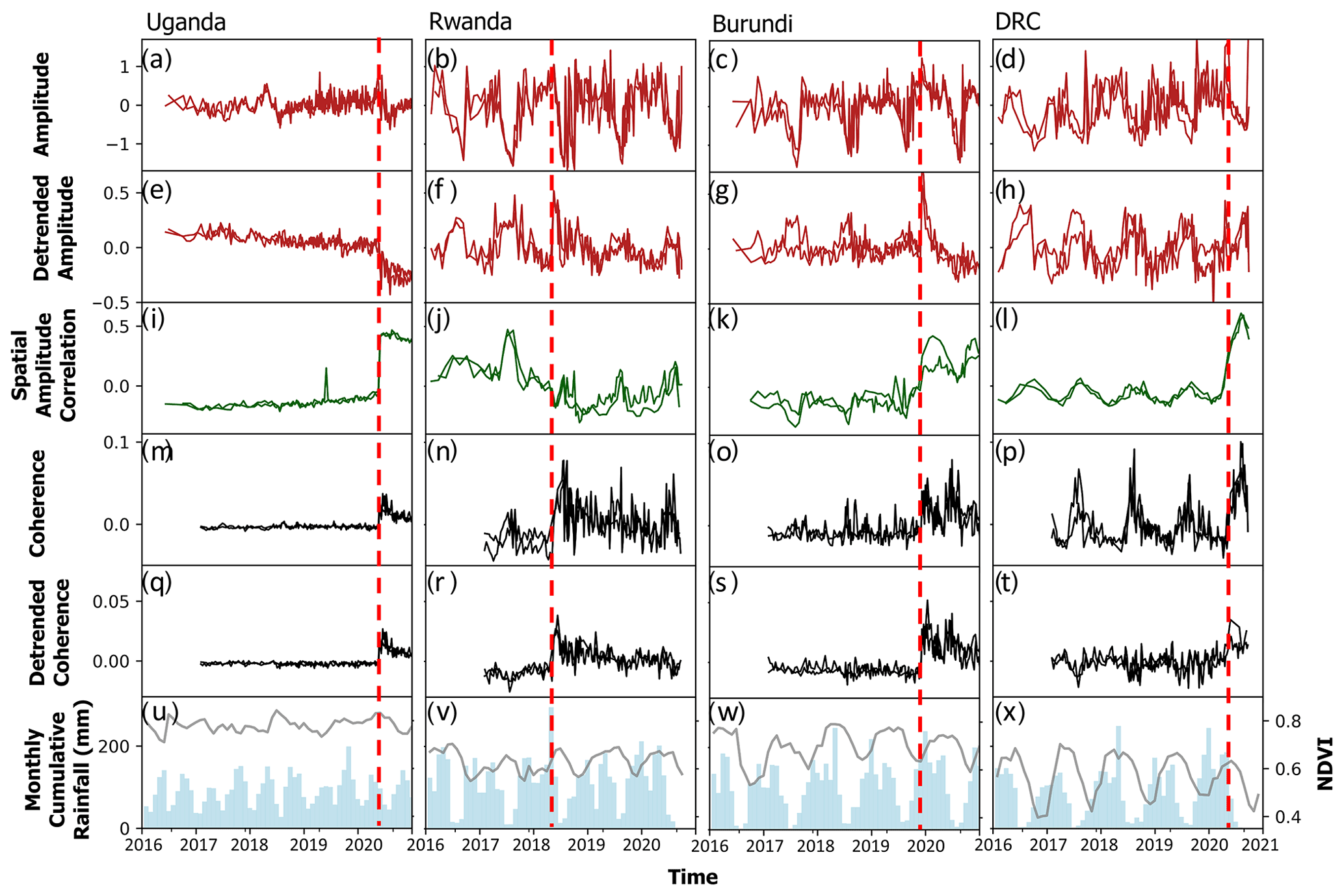
Figure 6GH event (detrended) amplitude (red), spatial amplitude correlation (SAC, green), and (detrended) coherence (black) time series. The dashed red line represents the timing of the GH event occurrence within the time series. All coherence, amplitude, and SAC time series show two lines of a similar colour representing the ascending and descending track time series. The time series are created according to the complete GH event scale workflow described in Sect. 3.3. The bottom row shows the monthly cumulative precipitation (light-blue bars) from IMERG satellite data and the monthly averaged NDVI values (grey line) from Landsat 8 (method described in Sect. 2.3).
The distinctiveness of the GH event occurrence within the time series varies significantly per data product (Fig. 6). SAC (Fig. 6i–l) and coherence (Fig. 6m–t) time series showcase the timing of the event with a significant change of value at the time of the event occurrence. A significant decrease in co-event (the coherence value from the pre- and post-event image) coherence is not visible.
The amplitude time series do not show any distinct change at the time of the GH event occurrence (Fig. 6a–h) except for the Uganda GH event (Fig. 6a and e). Particularly in the amplitude time series, and to a minor extent in the coherence time series, clear cyclicity can be observed that corresponds with the two drier periods (December–February and June–August) that are prevalent in the region (Bonfils, 2012; Nicholson, 2017; Monsieurs et al., 2018a). The NDVI shows seasonal correlation with the precipitation patterns, where NDVI patterns follow precipitation patterns with a short time lag (Fig. 6u–x). Stronger NDVI variations align with a stronger cyclicity within the amplitude, SAC, and coherence time series, which is particularly visible when comparing the Uganda GH event (weak amplitude SAC and coherence cyclicity, limited NDVI fluctuations) and the DRC GH event (stronger amplitude, SAC, and coherence cyclicity, large NDVI fluctuations). The cyclicity clearly influences the distinctiveness of the GH event within the time series. When comparing the landscape of both GH events (Fig. 2a and d), a sharp contrast is observed. The Uganda GH event region is mostly covered by forest, whereas the DRC GH event region is mostly covered by grass- and cropland. Consequently, we find that seasonal NDVI oscillations vary significantly from one study area to another given the difference in landscape.
Time series detrending clearly reduces seasonal cyclicity within the time series, which is particularly visible for the coherence time series (Fig. 6q–t) and to a much smaller degree for the amplitude time series (Fig. 6e–h). For example, the DRC GH event coherence time series benefits from this detrending procedure such that seasonal cyclicity is almost completely removed, leaving a distinct increase in coherence values after the occurrence of the GH event (Fig. 6t). Detrending the amplitude time series shows a minor reduction in cyclicity, but the distinctiveness of the GH event within the time series remains low.
4.2 Geomorphic hazard event timing
Figure 7 shows the timing estimation at the GH event scale (timing workflow 1) from the (detrended) amplitude, SAC, and (detrended) coherence time series. The difference in days from the actual occurrence of the GH event is visualised by a range that incorporates the minimal uncertainty in timing estimation (Figs. 7 and 8; see Sect. 3.3). Timing estimations from the amplitude time series generally have lower accuracies with estimated timing ranging from a 46 d difference (Uganda, descending) to a 1000 d difference (Uganda, ascending). Estimations from the SAC time series range between a 1 d (Uganda) and an 85 d (Rwanda) difference, and estimations from the coherence time series range between a 1 d (Uganda) and a 47 d (Rwanda) difference. Highest accuracies are achieved with time series showing less seasonal fluctuation and a steep change at the time of event occurrence (Fig. 5). Timing estimations from the detrended amplitude time series show an increased accuracy compared to amplitude time series with the most significant change for the Uganda GH event from a 46–1000 to a 13–22 d difference, but performance is still poor and generally useless for accurate timing estimation. Detrending the coherence time series increases timing estimation accuracy compared to the non-detrended coherence timing estimation for the DRC event (25–32 to a 1–5 d difference), but in general the estimations remain the same.
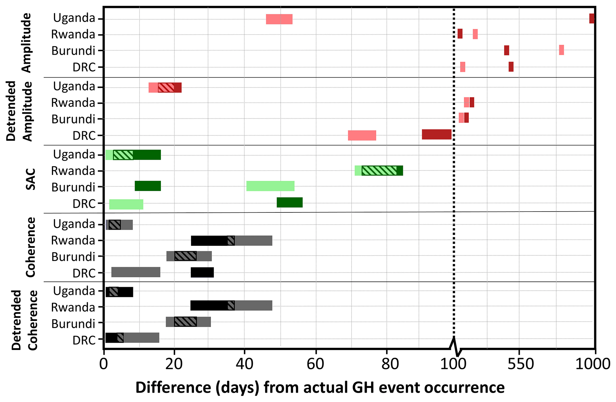
Figure 7Estimated GH event timing using the complete GH event scale (workflow 1) for amplitude, detrended amplitude (red), SAC (green), coherence, and detrended coherence (black). The darker coloured bar represents the ascending track results. The lighter coloured bar represents the descending track results. The length of bars represents the uncertainty in timing (see Sect. 3.3). Dashed lines on the bars represent the overlap between the ascending and descending track results.
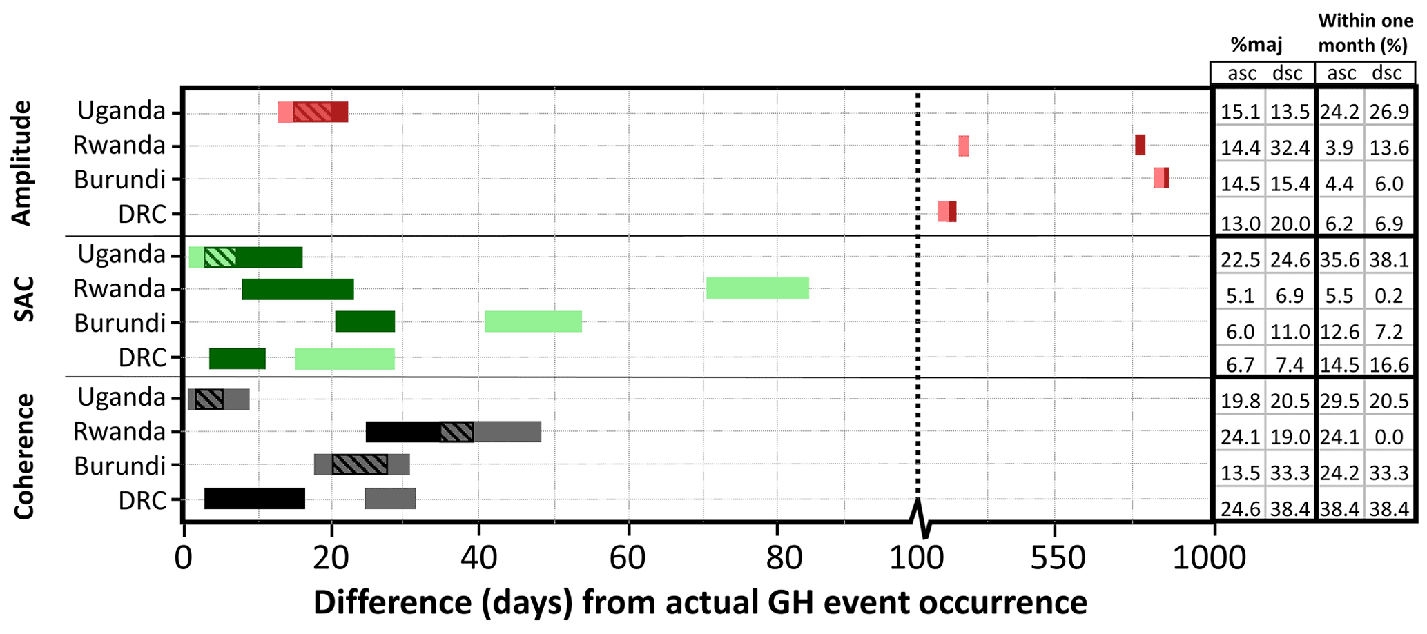
Figure 8Estimated timing from the individual GH feature scale (workflow 2) for amplitude, detrended amplitude (red), SAC (green), coherence, and detrended coherence (black). The darker coloured bar represents the ascending track results. The length of bars represent the uncertainty in timing (see Sect. 3.3). Dashed lines on the bars represent the overlap between the ascending and descending track results. In the % maj column we present the percentage of individual GH features over the total number of individual GH features that were included in the majority vote separated for the ascending (asc) and descending (dsc) track. In the “within one month” column we present the percentage of individual GH features over the total number of individual GH features that estimated a date within one month of the actual event occurrence.
Figure 8 shows the timing estimation based on the individual GH features within the GH event (timing workflow 2). Here, the estimated timing represents the date that is estimated most frequently between all individual GH features (as explained in Sect. 3.3). The percentage of individual GH features that estimate this (most frequently estimated) date over the total number of GH features (% maj) is shown in Fig. 8.
In general, timing estimations from the amplitude time series have low accuracies with estimated timing ranging from a 13 d difference to an 831 d difference. A distinct increase in accuracy is seen for the Uganda GH event compared to the GH event scale (Fig. 7). However, the other GH events do not show any distinct increase in timing estimation accuracy. The % maj ranges between 13 % and 32.4 % and shows that for some GH events, a large portion of the individual GH features estimate a date that is far from the actual date of the GH event occurrence. The percentage of individual GH features that estimate a date within 1 month of the actual GH event occurrence from amplitude time series is 24.2 % (ascending) and 26.9 % (descending) for the Uganda GH event, but much lower for the other GH events, corroborating the fact that the timing detection method performs poorly for the amplitude data product.
Timing estimations from the SAC time series from individual GH features (Fig. 8) differ compared to the timing estimations at the GH event scale (Fig. 7). An increase in accuracy is seen for Rwanda (ascending) and DRC (ascending), and a decrease in accuracy is seen for Burundi (ascending) and DRC (descending). The estimated timing ranges from a 1 d difference to an 85 d difference. Although estimated timing accuracy is higher for SAC compared to amplitude, % maj values are quite low, indicating weak estimations. The percentage of individual GH that estimates a date within one month of the actual GH event occurrence ranges from 0.2 (Rwanda, descending) to 38.1 (Uganda, descending). Exceptionally, for the Uganda GH event, % maj and estimated timing within one month of the GH event occurrence from the SAC time series is highest in comparison with amplitude and coherence (Fig. 8).
Timing estimations from the coherence time series from individual GH features (Fig. 8) are similar to those achieved at the GH event scale (Fig. 7) and have, generally, the highest accuracy for all data products. The % maj values ranged from 13.5 (Burundi, ascending) to 38.4 (DRC, descending). The percentage of individual GH features that estimates a date within one month of the actual GH event occurrence ranges from 0 (Rwanda, descending) to 38.4 (DRC, descending). The low percentages from the Rwanda descending track can be attributed to the fact that the estimated date is 37 d from the GH event occurrence and therefore just falls outside the 1-month threshold.
4.3 Sensitivity analysis with respect to landscape characteristics
GH size seems to have a clear influence on time estimation accuracy. Specifically, the SAC and coherence show a clear increase in percentages of estimated timing within 1 month of the GH event occurrence with increasing GH size (Fig. 9a–f). R2 values show a relatively reliable fit for both SAC and coherence. Amplitude shows a slight increasing trend, but associated R2 values are non-significant.
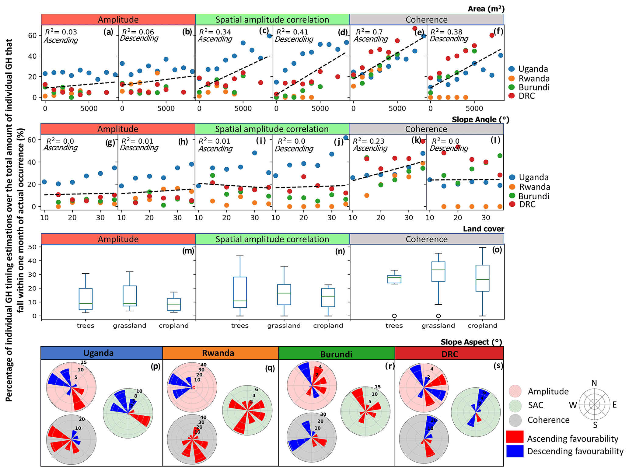
Figure 9Timing estimation performance over changing individual GH feature area (a–f), slope angle (g–l), land cover (m–o) and slope aspect (p–s). The y axis displays the percentage of individual GH features that estimated a timing that falls within one month of the actual GH event occurrence over the total number of individual GH features per GH event. Bin sizes: area = 1000 m, slope angle = 5∘, slope aspect = 45∘. Area (a–f) and slope angle (g–l) plots are separated per track, and the colours indicate the different GH events. The black dashed lines present the linear trend lines fitted to the data (a–l) for which the associated R2 values are included. Land cover (m–o): boxplots give lower and upper quartiles and median. The whiskers of each box represent 1.5 times the interquartile range. Outliers beyond whiskers are shown as dots. Slope aspect (p–s): the polar plots present the favourability of the ascending (ASC) or descending (DSC) track per slope aspect (see Sect. 4.3). The colour of the polar plot background indicates the SAR data product.
Slope trend lines (Fig. 9g–l) show in general little to no inclination and R2 values are non-significant, except for the coherence ascending track. Here, a clear increase in estimation accuracy becomes visible with increasing slope angle with a comparatively high R2 (although clearly less significant than R2 from the GH size analysis).
To assess the general influence of land cover on the ability to estimate GH event timing, we combined both the ascending and descending track results for all four GH events in each boxplot (Fig. 9m–o). Each boxplot therefore contains a total of eight data points per land cover type. The major land cover classes within the GH events were tree-covered area, grassland, and cropland (Fig. 4d). Median percentage values range around 9 %–10 % for amplitude, 11 %–16 % for SAC, and 27 %–34 % for coherence. Although median values within the grassland land cover type seem to be systematically higher among the three data products (amplitude, SAC, and coherence), differences with other land covers are quite small. No specific land cover shows a significant better performance.
To assess the influence of the slope orientation, we derive the difference between ascending and descending track percentages per bin and determine which track shows better performance (Fig. 9p–s). For the results of the Rwanda GH event (Fig. 9q), we see for SAC and coherence an all-round favourability for the ascending track, which can be explained by the fact that, like the results in Fig. 8, the Rwanda GH event had almost no estimations within one month of the GH event occurrence for the descending track. The results presented for Uganda, Burundi, and DRC GH events (Fig. 9p, r and s) show a general favourability of the ascending track for individual GH features that have an aspect of approximately 45–180∘, whereas a general favourability of the descending track for individual GH features that have an aspect of approximately 225–360∘. In contrast to this general trend, the opposite seems to be visible for the Uganda GH event coherence.
In this study we present a regionally applicable methodology to automatically determine GH event timing using S1 SAR data. Our study improves on the recent advances in GH event timing estimation research as (1) we are one of the firsts to use amplitude, SAC, and coherence time series in a systematic manner to detect the timing of GH events (Mondini et al., 2021); (2) we defined a methodology where no prior knowledge of the GH event timing is required; (3) we applied our methodology on contrasting landscapes, and (4) we combined, for the first time, landslides and flash floods in a single detection approach. Here we discuss our insights, results considering recent developments, and the potential improvements and future perspectives of our methodology.
5.1 Insights into geomorphic hazard event timing estimation from SAR
5.1.1 Geomorphic hazard event timing estimation
The use of amplitude or detrended amplitude time series in our methodology does not prove to be an effective approach to accurately determine the timing of GH events since it gives an estimation accuracy of 13 to 1000 d with the actual time occurrence of the events. A clear increase in accuracy is obtained from SAC with an accuracy of 1 to 85 d. However, the most accurate results are achieved with coherence and detrended coherence with a 1 to a 47 d accuracy.
GH event timing accuracies are higher for GH events that occurred in remote areas with low amounts of cultivation and human influence (highest accuracies for Uganda GH event, lowest for Rwanda GH event). The magnitude of the seasonal vegetation oscillations, which shows connectivity with the precipitation patterns (Fig. 6), varies significantly with changing landscapes and results in profound seasonal cyclicity in both the amplitude and coherence time series. Although the coherence is additionally influenced by atmospheric effects (Rocca et al., 2000), the influence of both the vegetation and atmosphere on the coherence does not obscure the GH-event-induced change within the time series. Notably, after detrending, the effects of both seem to be almost negligible. Denser and taller vegetation result in lower seasonal cyclicity within the amplitude and coherence time series. S1 operates in C-band frequency, meaning that the emitted signal penetrates the canopy layer and subsequently bounces on the branches and leaves underneath (Dzurisin, 2006). A reduction in vegetation after a seasonal dry period within sparsely vegetated areas, i.e. the grass- and croplands in the DRC GH event, will likely expose the soil underneath and have a pronounced influence on the backscattering signal given the difference in backscattering properties of vegetation and soil (Strozzi et al., 2000; Weydahl, 2001; Colesanti and Wasowski, 2006; Tessari et al., 2017). In contrast, a seasonal dry period in a dense forest (i.e. Uganda GH event) would affect the density of the canopy cover. However due to the height and close vicinity of the vegetation to each other a dry period does not necessarily lead to more soil exposure. This is corroborated by the fact that the NDVI does not change much for the Uganda GH event despite the seasonal patterns in precipitation (Fig. 6). The regions that are covered with the denser and most uniform vegetation are commonly environments with the lowest chance of getting timing information from other sources (media, citizen-observer networks) as compared to GH events in more inhabited landscapes (Jacobs et al., 2019; Monsieurs et al., 2019).
The complex reaction of the SAR signal to soil moisture and roughness change can cause both an increase and decrease of the amplitude at the same GH event location (Mondini et al., 2021; Burrows et al., 2022). Next to the seasonal influence (Fig. 6), this can also be a potential reason why no significant changes at the timing of the GH event are distinguished for all GH events. The inter-pixel variation captured in SAC proves to be a good tool to account for both this potential increase and decrease and any seasonal variation in amplitude values at the location of the GH event and increased timing estimation accuracy.
The pre-event, co-event, and post-event coherence values of our four GH events correspond with the study of Tzouvaras et al. (2020), where a distinct difference in pre- (low) and post- (high) GH event coherence values is observed at the location of a landslide occurrence. We observe the same patterns with the GH events that contain flash floods, likely because a clear landscape change is observed after the occurrence of the (often sediment-rich) flash floods (Fig. 1). The co-event coherence drop as observed by Tzouvaras et al. (2020) and Burrows et al. (2019) at the location of a landslide occurrence does not prove to be significant enough to be able to determine GH event timing. This is most likely attributed to the fact that the GH events occurred in low-coherence (vegetated) areas (Weydahl, 2001; Tessari et al., 2017).
5.1.2 Geomorphic hazard event distribution
An increase in GH area improves the accuracy of timing detection, which can likely be related to the increased number of pixels fully covering the GH feature relative to the fuzzy edge pixels (e.g. Foody and Mathur, 2006; Deijns et al., 2020; Zhong et al., 2021).
Generally, accuracy is not correlated with slope angle (Fig. 9). However, an increase in accuracy, with increasing slope, with a relative low reliability is observed for coherence. Nevertheless, this trend must be considered with a certain caution: (1) the trend is dependent on the quality of terrain correction during the pre-processing step (Sect. 3.1), which should make SAR values independent of slope angle (Small, 2011); (2) a changing slope angle could influence the GH size (Chen et al., 2016); and (3) we take the average slope angle per GH. Elongated GH features (mainly the flash flood features in the GH inventories) will have an average slope angle that is not representative of every part of the GH.
Although a clear difference can be observed in time series response to GH events located in different landscapes (Fig. 6), the comparison with the land cover does not allow for finding a clear relationship with the type of vegetation (Fig. 9). Since the land cover distribution is not equal amongst GH events (Fig. 5), the results are, for some GH events, based on a low number of individual GH features. The general trends could therefore also be influenced by additional underlying trends such as GH size and GH slope angle. The observed large variation in values per boxplot (Fig. 9m–o) might be an indication of this.
By using the right-looking S1 satellite data, foreshortening and layover effects should be limited with descending track acquisitions for GH exposed towards the west (180–360∘) and with ascending track acquisitions for GH exposed towards the east (0–180∘). The shadow affects in the opposite direction and is dependent on the slope of the terrain (Bamler, 2000). We see that, generally, the individual GH features on the west-facing slopes have higher timing estimation accuracies using the descending track imagery and the individual GH features on the east-facing slopes have higher timing estimation accuracies using the ascending track imagery, which is as expected.
However, there remains variability in the result; for example, an opposite pattern is visible for the Uganda GH event with the coherence and a partial favourability for the descending track acquisition on east-facing slopes is visible for the DRC GH event. Future research on the detailed effect of changing GH feature aspects on the ascending and descending SAR time series can provide additional valuable information in this context.
Our derived trends are established from GH events with each of the 318 to 1063 individual GH features and provide a good indication of the SAR response to changing landscape parameters. It remains interesting to see if these trends sustain with the addition of more GH events from different landscapes.
5.2 Result considering recent developments in SAR timing detection
Our results are somewhat in contrast with Burrows et al. (2022), who argue that coherence is less performant than amplitude for GH event timing. Using amplitude data, they were able to estimate the timing of ∼30 % of landslides per inventory with an accuracy of ∼80 % and an average precision of 12 d. Whereas by using coherence (60×60 m resolution) they acquired much less accurate results (24 %–47 % correctly estimated). Their study, however, differs in several aspects from our analysis:
-
Burrows et al. (2022) applied their method with a pre-defined notion of GH event timing, i.e. known year and season. For our GH events, we see distinct seasonal dynamics mainly within the amplitude time series. Zooming in on a specific time frame (3 months before and 3 months after the GH event occurrence like Burrows et al., 2022) reduces the overall seasonal dynamics, which could be the cause of a wrongly identified GH event change. Reducing this time window will potentially improve the detectability of the GH event within the time series. However, our methodology is intended to be applicable in areas such as the western branch of the East African Rift, an area characterised by data scarcity (Dewitte et al., 2021). In areas like these, information on the temporal distribution of GH events may not always be available. We therefore defined a methodology that requires no knowledge on GH event timing before application, which is an advantage if no GH event timing is present; however, this increases the chance of any seasonal influence visible within the time series.
-
They applied their method on landslides only. In our case, the addition of flash floods to the inventories introduces different types of contrasting GH shapes, slopes, and land cover (flash floods tend to be elongated and occur in the valleys with shallower terrain, whereas landslides occurred mainly on the steeper hillslopes) that can influence the SAR time series, specifically if the flash flood enters urbanised areas (such as in the DRC GH event) or run through a seasonally dynamic channel with seasonally changing soil moisture levels influencing the SAR signal (Ulaby et al., 1996; Scott et al., 2017).
-
Their used landslide inventories (from Roback et al., 2018, and Emberson et al., 2022) are located in densely vegetated areas (NDVI between 0.6 and 0.8). In agreement with Burrows et al. (2022) our results show that the Uganda GH event, where most of the landscape consists of dense vegetation (i.e. the highest NDVI values), estimated GH event timing accuracies are the highest among all GH events, obtaining a 1–2 image difference from the actual GH event occurrence for SAC (1–16 d) and (detrended) coherence (1–8 d). Although amplitude is overall less performant for the Uganda GH event, we still achieve an accuracy of 13–22 d for the detrended amplitude.
-
We do not threshold on individual GH area. Specifically, the Rwanda GH event contains a GH event size distribution that includes many small individual GH features below the threshold used in Burrows et al (2022) (Fig. 5). Together with the complexity and large fraction of cultivation of the landscape this clearly results in reduced estimation accuracies.
-
They removed landslide timing estimations using the magnitude of change caused by the landslide within the SAR time series, which allowed them to improve the estimation accuracy.
5.3 Improvements and perspectives
The current methodology successfully allows for analysing a GH event timing from SAR, but several improvements can be considered in future research.
5.3.1 Improvements
-
In the current methodology we do not detrend individual GH feature time series (see Sect. 3.3). Because detrending does increase timing accuracy within our study, further research on accurate detrending of individual GH time series can potentially greatly benefit timing estimation accuracy.
-
We use one change detection algorithm (ruptures: Truong et al., 2020) to estimate GH event timing. Comparing multiple change detection algorithms (e.g. Deijns et al., 2020; Burrows et al., 2022) could potentially benefit GH event timing estimation accuracy.
-
The quality of the amplitude and coherence imagery is dependent on the quality of the pre-processing applied with the MasTer tool (Derauw et al., 2020; d'Oreye et al., 2021) and how it deals with the different steps such as co-registration, radiometric terrain correction, and geocoding. Quality of the imagery in its turn is also dependent on, among others, the multi-look factor (amplitude), the interferometric multi-look factor, and the maximum temporal and perpendicular baselines (coherence). In addition, different polarisations may yield different results (Shibayama et al., 2015; Psomiadis, 2016; Park and Lee, 2019), and the use of a different polarisation can potentially improve event detectability within the time series. Improvements within the SAR imagery might be achieved by tweaking and closely investigating different pre-processing steps to achieve better image quality.
-
The SAC result depends on the ability to find the best reference image (Sect. 3.2). Additional efforts can be made to better find the SAC time series that shows the most significant change related to the GH event occurrence. For example, a preliminary filtering of very noisy SAC time series (before applying our developed method using the ECDFs) can potentially benefit the ability to acquire the best reference image.
5.3.2 Perspectives
-
We have studied, for the first time in a GH event timing detection approach, both landslides and flash floods in a combined methodology. Since these GHs often co-occur and interact (Marengo and Alves, 2012; Jacobs et al., 2016a; Rengers et al., 2016), they should be analysed in a multi-hazard approach. Our methodology can be well applied within such an approach. For example, multi-hazard inventories can serve as input for our methodology if there is a need to improve their timing accuracy. Results can subsequently be used in hazard assessment, early warning, and disaster risk reduction strategies.
-
Our study shows that there is a clear advantage to analysing different S1 SAR data products when estimating GH event timing. The fact that Burrows et al. (2022) show better results for amplitude compared to coherence data is in contrast with our results but reinforces the idea of investigating both data products when applying the methodology to new regions.
-
Given the clear influence of landscape and climate as controlling factors for SAR time series behaviour (Sect. 2.3), we aimed to develop our methodology within a variety of contrasting landscapes and contrasting vegetation dynamics. This offers perspectives for transferability. We show that slope angle does not seem to influence accuracy (Fig. 9). Based on landscape characteristics, transferability to other regions seems therefore likely to acquire good results, specifically for the SAC, coherence, and detrended coherence time series as they do seem less influenced by seasonal dynamics than the amplitude and detrended amplitude time series (Fig. 6). However, climate drivers could also potentially play a role. For example, since soil moisture and wetness have an influence on amplitude and coherence time series (Ulaby et al., 1996; Srivastava et al., 2006; Brancato et al., 2017; Scott et al., 2017), contrasting precipitation regimes within other regions could potentially influence the response of the SAR time series and the estimated GH event timing accuracy. Examples of contrasting precipitation regimes are (1) a lower amount of precipitation in more arid regions or lower/higher amounts in other tropical regions (Fick and Hijmans, 2017), (2) a change in precipitation seasonal variability due to spatially different oscillation of the ITCZ (Nicholson, 2017; Dewitte et al., 2022), and (3) the effect of local topography and the presence of lakes on the local precipitation patterns (e.g. Thiery et al., 2015, 2016, 2017; Monsieurs et al., 2018b). The influences of these contrasting precipitation regimes on SAR-based GH timing detection, however, remains to be investigated. Additionally, in its current form, the methodology does not account for the GH events that occur within a time span that is longer than the acquisition time (>6–12 d) of S1 images (i.e. multi-temporal GH events). In that case one would require a time window of occurrence, rather than a specific date. The methodology can be adapted to allow for it to derive a time window of GH occurrence. This could mainly be done following the GH event scale, where the start and the end date of the GH event inducing change within the SAR time series (applicable for all data products) should be indicative of the time window of GH event occurrence. However, this remains to be investigated.
-
The open-access S1 satellite with its high resolution, high repeat time, and global coverage proves to be an excellent data product for estimating GH event timing and allows for our developed methodology to be applied on every region of the world. The use of our methodology with different satellite products (e.g. Constellation of small Satellites for the Mediterranean basin Observation-SkyMed (COSMO-SkyMed), upcoming NASA–Indian Space Research Organisation SAR (NISAR) satellite) is not straightforward. Different available SAR satellite products operate in different bands with their own characteristics (e.g. X-band for COSMO-SkyMed; Covello et al., 2010, L-band for NISAR; NISAR, 2018) that will likely have implications on the ability for accurate GH event timing estimation. For example, the varying vegetation penetration depths associated with different SAR bands (Dzurisin, 2006) will likely have an influence on the impact of seasonal vegetation dynamics on the SAR time series as observed for our GH events (Fig. 6).
-
The methodology can benefit (in terms of data availability, scalability, and processing time) from implementation on a cloud computing service. Cloud computing platforms such as GEE only provide pre-processed amplitude imagery (i.e. amplitude ground range detected imagery). As such, they allow for the applicability of our methodology using the amplitude, detrended amplitude, and SAC data products. To our knowledge, so far, no cloud computing platform offers the possibility for processing and using coherence data. Additionally, the use of pre-processed amplitude imagery restrains us from manual input during the pre-processing step (as the MasTer Toolbox allows).
-
The methodology can potentially be combined with optical data (e.g. Deijns et al., 2020) that could serve as additional data to help narrow down the time window and filter out any nonsense timing estimations.
We established a regionally applicable methodology to automatically determine GH event timing from SAR images that can be applied without prior knowledge of the GH event. We successfully assessed the use of multiple SAR-derived data products in their ability to accurately detect GH event timing in contrasting landscapes. We show that landslides and flash floods can be detected and studied together; hence, we open new perspectives in the study of multi-hazards that can subsequently aid in hazard assessment, early warning, and disaster risk reduction strategies. Our methodology has the potential to be combined with existing spatial detection methods to support inventory creation and boost GH event research in remote inaccessible areas such as the African cloud-covered tropics.
From a data processing point of view, the methodology is established around an unprecedented analysis of various SAR products coming from Sentinel-1 (S1) images. We show that there is a need to investigate different SAR data products when estimating GH event timing (amplitude, spatial amplitude correlation, and coherence) since the signal response can be different and sometimes contradictory when looking at one single event. The implementation of our methodology on a cloud computing platform can be beneficial in terms of scalability, data availability, and processing time. However, the main limitations in this context are (1) no control in pre-processing of S1 imagery and (2) S1 coherence data are so far not available within these platforms.
With a focus on four events containing a total of about 2500 landslides and flash flood features in contrasting landscapes, we propose a methodology that is adapted to be applied to other regions. Here, we focused on tropical environments where climate conditions and land use dynamics are rather specific. However, we believe that the complexity of these landscapes is an added value for the transferability of the methodology. Additionally, the use of the globally available open-access S1 satellite data allows our methodology to be applied on every region of the world.
Sentinel-1 data are provided open access by ESA and retrieved from ASF DAAC (https://search.asf.alaska.edu/#/; Copernicus, 2022a). Sentinel-2 data are provided open access by ESA and retrieved from Google Earth Engine (https://developers.google.com/earth-engine/datasets; Copernicus, 2022b). Landsat 8 data are provided open access by the US Geological Survey and retrieved from Google Earth Engine (https://developers.google.com/earth-engine/datasets; US Geological Survey, 2022). The Python scripts for the GH event timing estimation, sensitivity analysis, and precipitation analysis and the Google Earth Engine code for vegetation analysis can be accessed at https://doi.org/10.5281/zenodo.7198346 (Deijns, 2022a). The four GH inventories can be downloaded at https://doi.org/10.5281/zenodo.7198322 (Deijns, 2022b).
AAJD, OD, FK, and WT conceived the study. AAJD compiled the landslide and flash flood inventory with the support of OD. AAJD processed and analysed the data. OD conducted field-work for the validation of the inventory. AAJD wrote the original draft of the manuscript, with key initial input from OD and FK. NO trained AAJD in SAR image pre-processing. All the authors contributed to reviewing and editing the manuscript. OD obtained funding for this work.
The contact author has declared that none of the authors has any competing interests.
Publisher's note: Copernicus Publications remains neutral with regard to jurisdictional claims in published maps and institutional affiliations.
This study was supported by the Belgian Science Policy Office (BELSPO) through the PAStECA project (BR/165/A3/PASTECA) entitled “Historical Aerial Photographs and Archives to Assess Environmental Changes in Central Africa” (http://pasteca.africamuseum.be, last access: 7 November 2022) and the GEOTROP project (B2/223/P1/GEOTROP) entitled “GEOmorphic hazards and compound events in a changing Tropical East Africa”. The compilation of the inventory data benefited from field-based insight and discussion with Arthur Depicker, Josué Mugisho Bachinyaga, John Sekajugo, and Judith Uwihirwe. PlanetScope data provided by the European Space Agency.
This research has been supported by the Belgian Federal Science Policy Office through two grants (grant nos. BR/165/A3/PASTECA and B2/223/P1/GEOTROP).
This paper was edited by Filippo Catani and reviewed by two anonymous referees.
Aimaiti, Y., Liu, W., Yamazaki, F., and Maruyama, Y.: Earthquake-induced landslide mapping for the 2018 Hokkaido Eastern Iburi earthquake using PALSAR-2 data, Remote Sens., 111, 2351, https://doi.org/10.3390/rs11202351, 2019.
Ali, K., Bajracharyar, R. M., and Raut, N.: Advances and challenges in flash flood risk assessment: A review, J. Geogr. Nat. Disast., 7, 1–6, https://doi.org/10.4172/2167-0587.1000195, 2017.
Bai, J.: Estimating multiple breaks one at a time, Econ. Theory, 13, 315–352, https://doi.org/10.1017/S0266466600005831, 1997.
Balzter, H.: Forest mapping and monitoring with interferometric synthetic aperture radar (InSAR), Prog. Phys. Geogr., 25, 159–177, https://doi.org/10.1177/030913330102500201, 2001.
Bamler, R.: Principles of synthetic aperture radar, Surv. Geophys., 21, 147–157, https://doi.org/10.1023/A:1006790026612, 2000.
Barrett, B., Whelan, P., and Dwyer, E.: The use of C-and L-band repeat-pass interferometric SAR coherence for soil moisture change detection in vegetated areas, Open Remote Sens. J., 5, 37–53, https://doi.org/10.2174/1875413901205010037, 2012.
Behling, R., Roessner, S., Kaufmann, H., and Kleinschmit, B.: Automated spatiotemporal landslide mapping over large areas using rapideye time series data, Remote Sens., 6, 8026–8055, https://doi.org/10.3390/rs6098026, 2014.
Behling, R., Roessner, S., Golovko, D., and Kleinschmit, B.: Derivation of long-term spatiotemporal landslide activity – A multi-sensor time series approach, Remote Sens. Environ., 186, 88–104, https://doi.org/10.1016/j.rse.2016.07.017, 2016.
Bonfils, S.: Trend analysis of the mean annual temperature in Rwanda during the last fifty two years, J. Environ. Protect., 3, 20077, https://doi.org/10.4236/jep.2012.36065, 2012.
Bradshaw, C. J. A., Sodhi, N. S., Peh, K. S. H., and Brook, B. W.: Global evidence that deforestation amplifies flood risk and severity in the developing world, Global Change Biol., 13, 2379–2395, https://doi.org/10.1111/j.1365-2486.2007.01446.x, 2007.
Brancato, V., Liebisch, F., and Hajnsek, I.: Impact of plant surface moisture on differential interferometric observables: A controlled electromagnetic experiment, IEEE T. Geosci. Remote, 55, 3949–3964, https://doi.org/10.1109/TGRS.2017.2684814, 2017.
Burrows, K., Walters, R. J., Milledge, D., Spaans, K., and Densmore, A. L.: A new method for large-scale landslide classification from satellite radar, Remote Sens., 11, 237, https://doi.org/10.3390/rs11030237, 2019.
Burrows, K., Walters, R. J., Milledge, D., and Densmore, A. L.: A systematic exploration of satellite radar coherence methods for rapid landslide detection, Nat. Hazards Earth Syst. Sci., 20, 3197–3214, https://doi.org/10.5194/nhess-20-3197-2020, 2020.
Burrows, K., Marc, O., and Remy, D.: Using Sentinel-1 radar amplitude time series to constrain the timings of individual landslides: a step towards understanding the controls on monsoon-triggered landsliding, Nat. Hazards Earth Syst. Sci., 22, 2637–2653, https://doi.org/10.5194/nhess-22-2637-2022, 2022.
Casagli, N., Frodella, W., Morelli, S., Tofani, V., Ciampalini, A., Intrieri, E., Raspini, F., Rossi, G., Tanteri, L., and Lu, P.: Spaceborne, UAV and ground-based remote sensing techniques for landslide mapping, monitoring and early warning, Geoenviron. Disast., 4, 9, https://doi.org/10.1186/s40677-017-0073-1, 2017.
Chen, X. L., Liu, C. G., Chang, Z. F., and Zhou, Q.: The relationship between the slope angle and the landslide size derived from limit equilibrium simulations, Geomorphology, 253, 547–550, https://doi.org/10.1016/j.geomorph.2015.01.036, 2016.
Colesanti, C. and Wasowski, J.: Investigating landslides with space-borne Synthetic Aperture Radar (SAR) interferometry, Eng. Geol., 88, 173–199, https://doi.org/10.1016/j.enggeo.2006.09.013, 2006.
Covello, F., Battazza, F., Coletta, A., Lopinto, E., Fiorentino, C., Pietranera, L., Valentini, G., and Zoffoli, S.: COSMO-SkyMed an existing opportunity for observing the Earth, J. Geodyn., 49, 171–180, https://doi.org/10.1016/j.jog.2010.01.001, 2010.
Copernicus: Sentinel-1: Copernicus Sentinel data, ASF DAAC [data set], https://search.asf.alaska.edu/#/ (last access: 7 November 2022), 2022a.
Copernicus: Sentinel-2: Copernicus Sentinel data, Google Earth Engine, https://developers.google.com/earth-engine/datasets (last access: 7 November 2022), 2022b.
Deijns, A. A. J.: Deijns et al. NHESS – SAR Timing – Scripts, Zenodo [code], https://doi.org/10.5281/zenodo.7198346, 2022a.
Deijns, A. A. J.: Deijns et al. NHESS – SAR Timing – GH Event Inventories, Zenodo [data set], https://doi.org/10.5281/zenodo.7198322, 2022b.
Deijns, A. A. J., Bevington, A. R., van Zadelhoff, F., de Jong, S. M., Geertsema, M., and McDougall, S.: Semi-automated detection of landslide timing using harmonic modelling of satellite imagery, Buckinghorse River, Canada, Int. J. Appl. Earth Obs. Geoinf., 84, 101943, https://doi.org/10.1016/j.jag.2019.101943, 2020.
Depicker, A., Jacobs, L., Mboga, N., Smets, B., Van Rompaey, A., Lennert, M., Wolff, E., Kervyn, F., Michellier, C., Dewitte, O., and Govers, G.: Historical dynamics of landslide risk from population and forest-cover changes in the Kivu Rift, Nat. Sustain., 4, 965–974, https://doi.org/10.1038/s41893-021-00757-9, 2021.
Derauw, D., Libert, L., Barbier, C., Orban, A., Kervyn, F., Samsonov, S., and d'Oreye, N.: The CSL InSAR Suite processor: specificities of a command line InSAR processing software specifically adapted for automated time series processing, in: ESA Living Planet Symposium 2019, 13–17 May 2019, Milano, Italy, https://lps19.esa.int/NikalWebsitePortal/living-planet-symposium-2019/lps19/Agenda/AgendaItemDetail?id=f879ca21-f0cf-4800-9473-e6882c23016d (last access: 7 November 2022), 2019.
Derauw, D., Jaspard, M., Caselli, A., and Samsonov, S.: Ongoing automated ground deformation monitoring of Domuyo-Laguna del Maule area (Argentina) using Sentinel-1 MSBAS time series: Methodology description and first observations for the period 2015–2020, J. S. Am. Earth Sci., 104, 102850, https://doi.org/10.1016/j.jsames.2020.102850, 2020
DeVries, B., Huang, C., Armston, J., Huang, W., Jones, J. W., and Lang, M. W.: Rapid and robust monitoring of flood events using Sentinel-1 and Landsat data on the Google Earth Engine, Remote Sens. Environ., 240, 111664, https://doi.org/10.1016/j.rse.2020.111664, 2020.
Dewitte, O., Dille, A., Depicker, A., Kubwimana, D., Maki Mateso, J.-C., Mugaruka Bibentyo, T., Uwihirwe, J., and Monsieurs, E.: Constraining landslide timing in a data-scarce context: from recent to very old processes in the tropical environment of the North Tanganyika-Kivu Rift region, Landslides, 18, 161–177, https://doi.org/10.1007/s10346-020-01452-0, 2021.
Dewitte, O., Depicker, A., Moeyersons, J., and Dille, A.: Mass Movements in Tropical Climates: Treatise on Geomorphology, in: vol. 5, edited by: Shroder, J. J. F., Elsevier, Academic Press, 338–349, https://doi.org/10.1016/B978-0-12-818234-5.00118-8, 2022.
Dobson, M. C. and Ulaby, F. T.: Active microwave soil moisture research, IEEE T. Geosci. Remote, 1, 23–36, https://doi.org/10.1109/TGRS.1986.289585, 1986.
d'Oreye, N., Derauw, D., Libert, L., Samsonov, S., Dille, A., Nobile, A., Monsieurs, E., Dewitte, O., and Kervyn, F.: Automatization of InSAR mass processing using CSL InSAR Suite (CIS) software for Multidimensional Small Baseline Subset (MSBAS) analysis: example combining Sentinel-1 and Cosmo-SkyMed SAR data for landslides monitoring in South Kivu, DR Congo, in: ESA Living Planet Symposium, 13–17 May 2019, Milano, Italy, https://lps19.esa.int/NikalWebsitePortal/living-planet-symposium-2019/lps19/Agenda/AgendaItemDetail?id=f879ca21-f0cf-4800-9473-e6882c23016d (last access: 7 November 2022), 2019.
d'Oreye, N., Derauw, D., Samsonov, S., Jaspard, M., and Smittarello, D.: MasTer: A Full Automatic Multi-Satellite InSAR Mass Processing Tool for Rapid Incremental 2D Ground Deformation Time Series, in: Int. Geosci. Remote Sens. Symp. (IGARSS), 12–16 July 2021, Brussels, 1899–1902, https://doi.org/10.1109/IGARSS47720.2021.9553615, 2021.
Dubois, P. C., Van Zyl, J., and Engman, T.: Measuring soil moisture with imaging radars, IEEE T. Geosci. Remote, 33, 915–926, https://doi.org/10.1109/36.406677, 1995.
Dzurisin, D.: Volcano deformation: new geodetic monitoring techniques, Springer, https://doi.org/10.1007/978-3-540-49302-0, 2006.
Emberson, R., Kirschbaum, D., and Stanley, T.: New global characterisation of landslide exposure, Nat. Hazards Earth Syst. Sci., 20, 3413–3424, https://doi.org/10.5194/nhess-20-3413-2020, 2020.
Emberson, R., Kirschbaum, D. B., Amatya, P., Tanyas, H., and Marc, O.: Insights from the topographic characteristics of a large global catalog of rainfall-induced landslide event inventories, Nat. Hazards Earth Syst. Sci., 22, 1129–1149, https://doi.org/10.5194/nhess-22-1129-2022, 2022.
ESA: Climate Change Initiative–Land Cover Project 2017, 20 m Resolution, European Space Agency, https://2016africalandcover20m.esrin.esa.int/ (last access: 7 November 2022), 2016.
Esposito, G., Marchesini, I., Mondini, A. C., Reichenbach, P., Rossi, M., and Sterlacchini, S.: A spaceborne SAR-based procedure to support the detection of landslides, Nat. Hazards Earth Syst. Sci., 20, 2379–2395, https://doi.org/10.5194/nhess-20-2379-2020, 2020.
Fick, S. E. and Hijmans, R. J.: WorldClim 2: new 1-km spatial resolution climate surfaces for global land areas, Int. J. Climatol., 37, 4302–4315, https://doi.org/10.1002/joc.5086, 2017.
Foga, S., Scaramuzza, P. L., Guo, S., Zhu, Z., Dilley Jr., R. D., Beckmann, T., Schmidt, G. L., Dwyer, J. L., Hughes, M. J., and Laue, B.: Cloud detection algorithm comparison and validation for operational Landsat data products, Remote Sens. Environ., 194, 379–390, https://doi.org/10.1016/j.rse.2017.03.026, 2017.
Foody, G. M. and Mathur, A.: The use of small training sets containing mixed pixels for accurate hard image classification: Training on mixed spectral responses for classification by a SVM, Remote Sens. Environ., 103, 179–189, https://doi.org/10.1016/j.rse.2006.04.001, 2006.
Froude, M. J. and Petley, D. N.: Global fatal landslide occurrence from 2004 to 2016, Nat. Hazards Earth Syst. Sci., 18, 2161–2181, https://doi.org/10.5194/nhess-18-2161-2018, 2018.
Fryzlewicz, P.: Wild binary segmentation for multiple change-point detection, Ann. Stat., 42, 2243–2281, https://doi.org/10.1214/14-AOS1245, 2014.
Ge, P., Gokon, H., Meguro, K., and Koshimura, S.: Study on the intensity and coherence information of high-resolution ALOS-2 SAR images for rapid massive landslide mapping at a pixel level, Remote Sens., 11, 2808, https://doi.org/10.3390/rs11232808, 2019.
Giertz, S., Junge, B., and Diekkrüger, B.: Assessing the effects of land use change on soil physical properties and hydrological processes in the sub-humid tropical environment of West Africa, Phys. Chem. Earth, 30, 485–496, https://doi.org/10.1016/j.pce.2005.07.003, 2005.
Gorelick, N., Hancher, M., Dixon, M., Ilyushchenko, S., Thau, D., and Moore, R.: Google Earth Engine: Planetary-scale geospatial analysis for everyone, Remote Sens. Environ., 202, 18–27, https://doi.org/10.1016/j.rse.2017.06.031, 2017.
Guzzetti, F., Peruccacci, S., Rossi, M., and Stark, C. P.: he rainfall intensity–duration control of shallow landslides and debris flows: an update, Landslides, 5, 3–17, https://doi.org/10.1007/s10346-007-0112-1, 2008.
Guzzetti, F., Mondini, A. C., Cardinali, M., Fiorucci, F., Santangelo, M., and Chang, K.-T.: Landslide inventory maps: New tools for an old problem, Earth-Sci. Rev., 112, 42–66, https://doi.org/10.1016/j.earscirev.2012.02.001, 2012.
Guzzetti, F., Gariano, S. L., Peruccacci, S., Brunetti, M. T., Marchesini, I., Rossi, M., and Melillo, M.: Geographical landslide early warning systems, Earth-Science Rev., 200, 102973, https://doi.org/10.1016/j.earscirev.2019.102973, 2020.
Hagberg, J. O., Ulander, L. M., and Askne, J.: Repeat-p–340, https://doi.org/10.1109/TGRS.1995.8746014, 1995.
Handwerger, A. L., Huang, M.-H., Jones, S. Y., Amatya, P., Kerner, H. R., and Kirschbaum, D. B.: Generating landslide density heatmaps for rapid detection using open-access satellite radar data in Google Earth Engine, Nat. Hazards Earth Syst. Sci., 22, 753–773, https://doi.org/10.5194/nhess-22-753-2022, 2022.
Hanssen, R. F.: Radar interferometry: data interpretation and error analysis, in: vol. 2, Springer, https://doi.org/10.1007/0-306-47633-9, 2001.
Heri-Kazi, A. B. and Bielders, C. L.: Cropland characteristics and extent of soil loss by rill and gully erosion in smallholder farms in the KIVU highlands, D. R. Congo, Geoderma Reg., 26, e00404, https://doi.org/10.1016/j.geodrs.2021.e00404, 2021.
Intrieri, E., Raspini, F., Fumagalli, A., Lu, P., Del Conte, S., Farina, P., Allievi, J., Ferretti, A., and Casagli, N.: The Maoxian landslide as seen from space: detecting precursors of failure with Sentinel-1 data, Landslides, 15, 123–133, https://doi.org/10.1007/s10346-017-0915-7, 2018.
Jacobs, L., Maes, J., Mertens, K., Sekajugo, J., Thiery, W., Van Lipzig, N., Poesen, J., Kervyn, M., and Dewitte, O.: Reconstruction of a flash flood event through a multi-hazard approach: focus on the Rwenzori Mountains, Uganda, Nat. Hazards, 84, 851–876, https://doi.org/10.1007/s11069-016-2458-y, 2016a.
Jacobs, L., Dewitte, O., Poesen, J., Delvaux, D., Thiery, W., and Kervyn, M.: The Rwenzori Mountains, a landslide-prone region?, Landslides, 13, 519–536, https://doi.org/10.1007/s10346-015-0582-5, 2016b.
Jacobs, L., Kabaseke, C., Bwambale, B., Katutu, R., Dewitte, O., Mertens, K., Maes, J., and Kervyn, M.: The geo-observer network: A proof of concept on participatory sensing of disasters in a remote setting, Sci. Total Environ., 670, 245–261, https://doi.org/10.1016/j.scitotenv.2019.03.177, 2019.
Jacquemart, M. and Tiampo, K.: Leveraging time series analysis of radar coherence and normalized difference vegetation index ratios to characterize pre-failure activity of the Mud Creek landslide, California, Nat. Hazards Earth Syst. Sci., 21, 629–642, https://doi.org/10.5194/nhess-21-629-2021, 2021.
Joyce, K. E., Belliss, S. E., Samsonov, S. V., McNeill, S. J., and Glassey, P. J.: A review of the status of satellite remote sensing and image processing techniques for mapping natural hazards and disasters, Prog. Phys. Geogr., 33, 183–207, https://doi.org/10.1177/0309133309339563, 2009.
Jung, J. and Yun, S. H.: Evaluation of coherent and incoherent landslide detection methods based on Synthetic Aperture Radar for rapid response: A case study for the 2018 Hokkaido landslides, Remote Sens., 12, 265, https://doi.org/10.3390/rs12020265, 2020.
Kennedy, R. E., Yang, Z., Gorelick, N., Braaten, J., Cavalcante, L., Cohen, W. B., and Healey, S.: Implementation of the LandTrendr algorithm on google earth engine, Remote Sens., 10, 691, https://doi.org/10.3390/rs10050691, 2018.
Kjekstad, O. and Highland, L.: Economic and Social Impacts of Landslides, in: Landslides – Disaster Risk Reduction, edityed by: Sassa, K. and Canuti, P., Springer, Berlin, Heidelberg, https://doi.org/10.1007/978-3-540-69970-5_30, 2009.
Komac, M., Holley, R., Mahapatra, P., van der Marel, H., and Bavec, M.: Coupling of GPS/GNSS and radar interferometric data for a 3D surface displacement monitoring of landslides, Landslides, 12, 241–257, https://doi.org/10.1007/s10346-014-0482-0, 2015.
Konishi, T. and Suga, Y.: Landslide detection using COSMO-SkyMed images: A case study of a landslide event on Kii Peninsula, Japan, Eur. J. Remote Sens., 51, 205–221, https://doi.org/10.1080/22797254.2017.1418185, 2018.
Korup, O., Densmore, A. L., and Schlunegger, F.: The role of landslides in mountain range evolution, Geomorphology, 120, 77–90, https://doi.org/10.1016/j.geomorph.2009.09.017, 2010.
Kubwimana, D., Ait Brahim, L., Nkurunziza, P., Dille, A., Depicker, A., Nahimana, L., Abdelouafi, A., and Dewitte, O.: Characteristics and Distribution of Landslides in the Populated Hillslopes of Bujumbura, Burundi, Geosciences, 11, 259, https://doi.org/10.3390/geosciences11060259, 2021.
Le Cozannet, G., Kervyn, M., Russo, S., Ifejika Speranza, C., Ferrier, P., Foumelis, M., Lopez, T., and Modaressi, H.: Space-Based Earth Observations for Disaster Risk Management, Surv. Geophys., 41, 1209–1235, https://doi.org/10.1007/s10712-020-09586-5, 2020.
Liu, C., Guo, L., Ye, L., Zhang, S., Zhao, Y., and Song, T.: A review of advances in China's flash flood early-warning system, Nat. Hazards, 92, 619–634, https://doi.org/10.1007/s11069-018-3173-7, 2018.
Marc, O., Stumpf, A., Malet, J.-P., Gosset, M., Uchida, T., and Chiang, S.-H.: Initial insights from a global database of rainfall-induced landslide inventories: the weak influence of slope and strong influence of total storm rainfall, Earth Surf. Dynam., 6, 903–922, https://doi.org/10.5194/esurf-6-903-2018, 2018.
Marengo, J. A. and Alves, L. M.: The 2011 intense rainfall and floods in Rio De Janeiro, B. Am. Meteorol. Soc., 93, 1–282, 2012.
Martinis, S., Kuenzer, C., Wendleder, A., Huth, J., Twele, A., Roth, A., and Dech, S.: Comparing four operational SAR-based water and flood detection approaches, Int. J. Remote Sens., 36, 3519–3543, https://doi.org/10.1080/01431161.2015.1060647, 2015.
Mohan, A., Singh, A. K., Kumar, B., and Dwivedi, R.: Review on remote sensing methods for landslide detection using machine and deep learning, Trans. Emerg. Telecommun. Technol. T., 32, 3998, https://doi.org/10.1002/ett.3998, 2021.
Mondini, A. C.: Measures of spatial autocorrelation changes in multitemporal SAR images for event landslides detection, Remote Sens., 9, 554, https://doi.org/10.3390/rs9060554, 2017.
Mondini, A. C., Santangelo, M., Rocchetti, M., Rossetto, E., Manconi, A., and Monserrat, O.: Sentinel-1 SAR amplitude imagery for rapid landslide detection, Remote Sens., 11, 760, https://doi.org/10.3390/rs11070760, 2019.
Mondini, A. C., Guzzetti, F., Chang, K. T., Monserrat, O., Martha, T. R., and Manconi, A.: Landslide failures detection and mapping using Synthetic Aperture Radar: Past, present and future, Earth-Sci. Rev., 216, 103574, https://doi.org/10.1016/j.earscirev.2021.103574, 2021.
Monsieurs, E.: The potential of satellite rainfall estimates in assessing regional landslide hazard in Central Africa, Doctoral dissertation, Université de Liège, Liège, Belgium, https://hdl.handle.net/2268/245576 (last access: 7 November 2022), 2020.
Monsieurs, E., Jacobs, L., Michellier, C., Basimike Tchangaboba, J., Bamulezi Ganza, G., Kervyn, F., Maki Mateso, J.-C., Mugaruka Bibentyo, T., Kalikone Buzera, C., Nahimana, L., Ndayisenga, A., Nkurunziza, P., Thiery, W., Demoulin, A., Kervyn, M., and Dewitte, O.: Landslide inventory for hazard assessment in a data-poor context: a regional-scale approach in a tropical African environment, Landslides, 15, 2195–2209, https://doi.org/10.1007/s10346-018-1008-y, 2018a.
Monsieurs, E., Kirschbaum, D. B., Tan, J., Maki Mateso, J.-C., Jacobs, L., Plisnier, P.-D., Thiery, W., Umutoni, A., Musoni, D., Mugaruka Bibentyo, T. Bamulezi Ganza, G., Ilombe Mawe, G., Bagalwa, L., Kankurize, C., Michellier, C., Stanley, T., Kervyn, F., Kervyn, M., Demoulin, A., and Dewitte, O.: Evaluating TMPA rainfall over the sparsely gauged East African Rift, J. Hydrometeorol., 19, 1507–1528, https://doi.org/10.1175/JHM-D-18-0103.1, 2018b.
Monsieurs, E., Dewitte, O., and Demoulin, A.: A susceptibility-based rainfall threshold approach for landslide occurrence, Nat. Hazards Earth Syst. Sci., 19, 775–789, https://doi.org/10.5194/nhess-19-775-2019, 2019.
Nakulopa, F., Vanderkelen, I., Van de Walle, J., Van Lipzig, N. P., Tabari, H., Jacobs, L., Tweheyo, C., Dewitte, O., and Thiery, W.: Evaluation of high-resolution precipitation products over the Rwenzori Mountains (Uganda), J. Hydrometeorol., 23, 747–768, https://doi.org/10.1175/JHM-D-21-0106.1, 2022.
Nicholson, S. E.: Climate and climatic variability of rainfall over eastern Africa, Rev. Geophys., 5, 590–635, https://doi.org/10.1002/2016RG000544, 201.
NISAR: NASA-ISRO SAR (NISAR) Mission Science Users' Handbook, NASA Jet Propulsion Laboratory, 261, 18–1893, https://nisar.jpl.nasa.gov/resources/documents (last access: 7 November 2022), 2018.
Nobile, A., Dille, A., Monsieurs, E., Basimike, J., Mugaruka Bibentyo, T., d'Oreye, N., Kervyn, F., and Dewitte, O.: Multi-temporal DInSAR to characterise landslide ground deformations in a tropical urban environment: Focus on Bukavu (DR Congo), Remote Sens., 10, 626, https://doi.org/10.3390/rs10040626, 2018.
Nolan, M. and Fatland, D. R.: Penetration depth as a DInSAR observable and proxy for soil moisture, IEEE T. Geosci. Remote, 41, 532–537, https://doi.org/10.1109/TGRS.2003.809931, 2003.
Park, S. E. and Lee, S. G.: On the use of single-, dual-, and quad-polarimetric SAR observation for landslide detection, ISPRS Int. J. Geo-Inf., 8, 384, https://doi.org/10.3390/ijgi8090384, 2019.
Petersen, M. S.: Impacts of Flash Floods. Coping With Flash Floods, in: NATO Science Series, vol. 77, edited by: Gruntfest, E. and Handmer, J., Springer, Dordrecht, https://doi.org/10.1007/978-94-010-0918-8_2, 2001.
Peterson, M., Mach, D., and Buechler, D.: A Global LIS/OTD Climatology of Lightning Flash Extent Density, J. Geophys. Res.-Atmos., 126, e2020JD033885, https://doi.org/10.1029/2020JD033885, 2021.
Planet Team: Planet Application Program Interface: In Space for Life on Earth, San Francisco, CA, https://api.planet.com (last access: 7 November 2022), 2017.
Psomiadis, E.: October. Flash flood area mapping utilising SENTINEL-1 radar data, Earth Resour. Environ. Remote Sens./GIS App. VII, 10005, 100051G, https://doi.org/10.1117/12.2241055, 2016.
Rengers, F. K., McGuire, L. A., Kean, J. W., Staley, D. M., and Hobley, D. E. J.: Model simulations of flood and debris flow timing in steep catchments after wildfire, Water Resour. Res., 52, 6041–6061, https://doi.org/10.1002/2015WR018176, 2016.
Roback, K., Clark, M. K., West, A. J., Zekkos, D., Li, G., Gallen, S. F., Chamlagain, D., and Godt, J. W.: The size, distribution, and mobility of landslides caused by the 2015 Mw 7.8 Gorkha earthquake, Nepal, Geomorphology, 301, 121–138, https://doi.org/10.1016/j.geomorph.2017.01.030, 2018.
Robinson, T. R., Rosser, N.,and Walters, R. J.: The Spatial and Temporal Influence of Cloud Cover on Satellite-Based Emergency Mapping of Earthquake Disasters, Sci. Rep. 9, 1–9, https://doi.org/10.1038/s41598-019-49008-0, 2019.
Rocca, F., Prati, C., Monti Guarnieri, A., and Ferretti, A.: SAR interferometry and its applications, Surv. Geophys., 21, 159–176, https://doi.org/10.1023/A:1006710731155, 2000.
Samsonov, S. and d'Oreye, N.: Multidimensional time-series analysis of ground deformation from multiple InSAR data sets applied to Virunga Volcanic Province, Geophys. J. Int., 191, 1095–1108, https://doi.org/10.1111/j.1365-246X.2012.05669.x, 2012.
Scott, C. P., Lohman, R. B., and Jordan, T. E.: InSAR constraints on soil moisture evolution after the March 2015 extreme precipitation event in Chile, Sci. Rep., 7, 1–9, https://doi.org/10.1038/s41598-017-05123-4, 2017.
Sekajugo, J., Kagoro-Rugunda, G., Mutyebere, R., Kabaseke, C., Namara, E., Dewitte, O., Kervyn, M., and Jacobs, L.: Can citizen scientists provide a reliable geo-hydrological hazard inventory? An analysis of biases, sensitivity and precision for the Rwenzori Mountains, Uganda, Environ. Res. Lett., 17, 045011, https://doi.org/10.1088/1748-9326/ac5bb5, 2022.
Shibayama, T., Yamaguchi, Y., and Yamada, H.: Polarimetric scattering properties of landslides in forested areas and the dependence on the local incidence angle, Remote Sens., 7, 15424–15442, https://doi.org/10.3390/rs71115424, 2015.
Small, D.: Flattening gamma: Radiometric terrain correction for SAR imagery, IEEE T. Geosci. Remote, 49, 3081–3093, https://doi.org/10.1109/TGRS.2011.2120616, 2011.
Solari, L., Del Soldato, M., Raspini, F., Barra, A., Bianchini, S., Confuorto, P., Casagli, N., and Crosetto, M. Review of satellite interferometry for landslide detection in Italy, Remote Sens., 12, 1351, https://doi.org/10.3390/rs12081351, 2020.
Srivastava, H. S., Patel, P., and Navalgund, R. R.: How far SAR has fulfilled its expectation for soil moisture retrieval, Microwave Remote Sens. Atmos. Environ., 6410, 641001 https://doi.org/10.1117/12.693946, 2006.
Strozzi, T., Dammert, P. B., Wegmuller, U., Martinez, J. M., Askne, J. I., Beaudoin, A., and Hallikainen, N. T.: Landuse mapping with ERS SAR interferometry, IEEE T. Geosci. Remote, 38, 766–775, https://doi.org/10.1109/36.842005, 2000.
Stumpf, A., Malet, J. P., Allemand, P., and Ulrich, P.: Surface reconstruction and landslide displacement measurements with Pléiades satellite images, ISPRS J. Photogram. Remote Sens., 95, 1–12, https://doi.org/10.1016/j.isprsjprs.2014.05.008, 2014.
Tessari, G., Floris, M., and Pasquali, P.: Phase and amplitude analyses of SAR data for landslide detection and monitoring in non-urban areas located in the North-Eastern Italian pre-Alps, Environ. Earth Sci., 76, 85, https://doi.org/10.1007/s12665-017-6403-5, 2017
Thiery, W., Davin, E. L., Panitz, H.-J., Demuzere, M., Lhermitte, S., and van Lipzig, N. P. M.: The impact of the African Great Lakes on the regional climate, J. Climate, 28, 4061–4085, https://doi.org/10.1175/JCLI-D-14-00565.1, 2015.
Thiery, W., Davin, E. L., Seneviratne, S. I., Bedka, K., Lhermitte, S., and van Lipzig, N. P. M.: Hazardous thunderstorm intensification over Lake Victoria, Nat. Comm., 7, 12786, https://doi.org/10.1038/ncomms12786, 2016.
Thiery, W., Gudmundsson, L., Bedka, K., Semazzi, F. H. M., Lhermitte, S., Willems, P., van Lipzig, N. P. M., and Seneviratne, S. I.: Early warnings of hazardous thunderstorms over Lake Victoria, Environ. Res. Lett., 12, 074012, https://doi.org/10.1088/1748-9326/aa7521, 2017.
Truong, C., Oudre, L., and Vayatis, N.: Selective review of offline change point detection methods, Signal Process., 167, 107299, https://doi.org/10.1016/j.sigpro.2019.107299, 2020.
Tucker, C. J.: Red and photographic infrared linear combinations for monitoring vegetation, Remote Sens. Environ., 8, 127–150, https://doi.org/10.1016/0034-4257(79)90013-0, 1979.
Turkington, T., Ettema, J., van Westen, C. J., and Breinl, K.: Empirical atmospheric thresholds for debris flows and flash floods in the southern French Alps, Nat. Hazards Earth Syst. Sci., 14, 1517–1530, https://doi.org/10.5194/nhess-14-1517-2014, 2014.
Twele, A., Cao, W., Plank, S., and Martinis, S.: Sentinel-1-based flood mapping: a fully automated processing chain, Int. J. Remote Sens., 37, 2990–3004, https://doi.org/10.1080/01431161.2016.1192304, 2016.
Tzouvaras, M., Danezis, C., and Hadjimitsis, D. G.: Small scale landslide detection using Sentinel-1 interferometric SAR coherence, Remote Sens., 12, 1560, https://doi.org/10.3390/rs12101560, 2020.
Ulaby, F. T., Dubois, P. C., and Van Zyl, J.: Radar mapping of surface soil moisture, J. Hydrol., 184, 57–84, https://doi.org/10.1016/0022-1694(95)02968-0, 1996.
US Geological Survey: Landsat 8 imagery, Google Earth Engine, US Geological Survey, https://developers.google.com/earth-engine/datasets, last access: 7 November 2022.
Van de Walle, J., Thiery, W., Brousse, O., Souverijns, N., Demuzere, M., and van Lipzig, N. P. M.: A convection-permitting model for the Lake Victoria Basin: Evaluation and insight into the mesoscale versus synoptic atmospheric dynamics, Clim. Dynam., 54, 1779–1799, https://doi.org/10.1007/s00382-019-05088-2, 2020.
van Westen, C. J., Castellanos, E., and Kuriakose, S. L.: Spatial data for landslide susceptibility, hazard, and vulnerability assessment: An overview, Eng. Geol., 102, 112–131, https://doi.org/10.1016/j.enggeo.2008.03.010, 2008.
Weydahl, D. J.: Analysis of ERS SAR coherence images acquired over vegetated areas and urban features, Int. J. Remote Sens., 22, 2811–2830, https://doi.org/10.1080/01431160010006412, 2001.
Zebker, H. A. and Villasenor, J.: Decorrelation in interferometric radar echoes, IEEE T. Geosci. Remote, 30, 950–959, https://doi.org/10.1109/36.175330, 1992.
Zhong, C., Li, C., Gao, P., and Li, H.: Discovering Vegetation Recovery and Landslide Activities in the Wenchuan Earthquake Area with Landsat Imagery, Sensors, 21, 5243, https://doi.org/10.3390/s21155243, 2021.