the Creative Commons Attribution 4.0 License.
the Creative Commons Attribution 4.0 License.
 | 21 Jul 2022
Predicting drought and subsidence risks in France
Arthur Charpentier
Molly James
Hani Ali
The economic consequences of drought episodes are increasingly important although they are often difficult to apprehend, in part because of the complexity of the underlying mechanisms. In this article we will study one of the consequences of drought, namely the risk of subsidence (or more specifically clay-shrinkage-induced subsidence), for which insurance has been mandatory in France for several decades. Using data obtained from several insurers, representing about a quarter of the household insurance market over the past 20 years, we propose some statistical models to predict not only the frequency but also the intensity of these droughts for insurers. But even if we use more advanced models than standard regression-type models (here random forests to capture non-linearity and cross effects) and all geophysical and climatic information is available, it is still difficult to predict the economic cost of subsidence claims.
- Article
(10686 KB) - Full-text XML
- BibTeX
- EndNote


Climate change is a challenge for the insurance industry since risks are increasing in terms of frequency and intensity, as discussed in McCullough (2004), Mills (2007), Charpentier (2008) or Schwarze et al. (2011). In this article, we will see if it is possible to predict for a given year the costs associated with drought and, more specifically here, clay-shrinkage-induced subsidence in France.
1.1 Droughts, economic impacts, insurance coverage and climate change
In a seminal book published 20 years ago, Bradford (2000) started to address the problem of obtaining a better understanding of the connections between drought and climate change, already suggesting that the frequency and the intensity of such events could increase in the future. And in a more recent book, Iglesias et al. (2019) provided additional evidence of the influence of climate change on meteorological droughts in Europe. Ionita and Nagavciuc (2021) studied the temporal evolution of three drought indexes over 120 years (the standardised precipitation index, SPI; the standardised precipitation evapotranspiration index, SPEI; and the self-calibrated Palmer drought severity index, scPDSI). This updated study regarding the trends and changes in drought frequency in Europe concluded that most of the severe drought events occurred in the last 2 decades, corresponding to the time after the publication of Lloyd-Hughes and Saunders (2002) for example. Similarly, Spinoni et al. (2015, 2017) (studying more specifically Europe, following their initial worldwide study in Spinoni et al., 2014) observed that for both frequency and severity, the evolution towards drier conditions has been more relevant in the last 3 decades over central Europe in spring, the Mediterranean area in summer and eastern Europe in autumn (also using multiple indexes, over 60 years).
Regarding economic impacts, Hagenlocher et al. (2019) present the outcomes of a systematic literature review, over the past 20 years, on people-centred drought vulnerability and risk conceptualisation and assessments. Despite major advances over the past decades in terms of developing better methods and tools for characterising individual components of risk, Hagenlocher et al. (2019) mentioned persistent knowledge gaps which need to be confronted in order to advance the understanding of drought risk for people and policymakers and move towards a more drought-resilient society. Naumann et al. (2021) show that (in Europe) drought damage, not related to subsidence or building damage but mainly agricultural losses, could strongly increase with global warming and cause a regional imbalance in future drought impacts. They provide some forecasts, under the assumption of absence of climate action (+4 ∘C in 2100 and no adaptation): annual drought losses in the European Union and United Kingdom combined are projected to rise to more than EUR 65 billion per year compared with EUR 9 billion per year currently, still “two times larger when expressed to the relative size of the economy” (expressed as a fraction of the GDP). Note that this corresponds to the general feeling of the insurance industry: Bevere and Weigel (2021) suggest that current drought trends and corresponding economic risks will be further aggravated under climate change.
But at the same time, Naumann et al. (2015) point out that related direct and indirect impacts are often difficult to quantify. A key issue is that the lack of sufficient quantitative impact data makes it complicated to construct a robust relationship between the severity of drought events and related damage. Insurance coverage for drought has been intensively studied when related to agriculture. Iglesias et al. (2019) mention some drought insurance schemes with both indemnity-based mechanisms and drought-index-based insurance, in Sect. 2.8. Vroege et al. (2019) provide an overview of index-based insurance in Europe and North America in the context of droughts, while Bucheli et al. (2021) focus on Germany. Note that Tsegai and Kaushik (2019) address the importance of designing insurance products which not only address drought impacts but also minimise land degradation. Besides this theoretical work, some countries provide actual cover for such risks. For example in Spain, it is possible to insure rain-fed crops against drought, as discussed in Entidad Estatal de Seguros Agrarios (2012), but in most countries drought coverage only concerns agricultural (crop) insurance in the same way that frost is covered (see also Pérez-Blanco et al., 2017).
1.2 From drought to subsidence
In this article we will use data from several insurance companies in France regarding a very specific drought-related peril, that is clay-shrinkage-induced subsidence, which causes damage to buildings. Without buildings to suffer from subsidence, there is no risk of damage. In turn, the risk of building damage is only part of the wider scope of the economic impacts of this (drought-induced) subsidence (as describe in Kok and Costa, 2021). If clay-shrinkage-induced subsidence is now a well-known peril (or at least recognised as a major peril; see for instance Doornkamp, 1993, or Brignall et al., 2002, which assessed the potential effects of climate change on clay-shrinkage-induced land subsidence), insurance coverage for subsidence is still uncommon. Almost 20 years ago, as indicated in McCullough (2004), while perils related to earth movement were traditionally excluded from most property policies, several states (in the United States of America) added mandated coverage for some subsidence-related claims (with several limitations). And recently, Herrera-García et al. (2021) proved that subsidence permanently reduces aquifer-system storage capacity, causes earth fissures, damages buildings and civil infrastructure, and increases flood susceptibility and risk. From an insurer's perspective, Wües et al. (2011) pointed out that as incidents of soil subsidence increase in frequency and severity with climate change, there is a need for systematic management of the risks through a combination of loss prevention and risk transfer initiatives (such as insurance).
In France, subsidence is a phenomenon covered by all private property insurance policies, and that enters the scope of the government-backed French natural catastrophe regime provided by the Caisse Centrale de Réassurance (CCR). It is the second-most-important peril in terms of costs that the system covers (the first being floods; see Charpentier et al., 2022, for a recent discussion about flood events in France, in the context of climate change). Subsidence risk is defined (Ministère de la transition écologique et solidaire, 2016) as the displacement of the ground surface due to shrinkage and swelling of clayey soils. It is due mainly to the presence of clay in the soil, which swells in humid conditions and shrinks in dry ones and thus creates instabilities in the terrain under constructions causing cracks to appear on the floor and in the walls which can jeopardise the solidity of the building. France, having a temperate climate, has saturated clayey soils, making subsidence predominant during droughts.
However, the past few years have seen this risk exacerbated by the extreme heatwaves and lack of rainfall in France (see Caisse Centrale de Réassurance, 2020), causing more and more subsidence claims with little hope of this tendency stopping given the current climate change context. Indeed, 37 % of the total costs of natural catastrophes in France between 1982 and 2020 are caused by subsidence, 38 % of which are concentrated over the period 2015–2019, which represents 15 % of the total time that subsidence coverage has been in place (as discussed in Mission des Risques Naturels, 2021). Furthermore, Soubeyroux et al. (2011) show that the frequency and intensity of heatwaves and droughts will inevitably increase in the coming century in continental France and new areas that so far have been protected from drought will be at risk. Additionally, the Association Française de l'Assurance (2015) predicts that the cost of geotechnical droughts will nearly triple in 2040. More recently, the French Geological Survey (BRGM, Bureau de Recherches Géologiques et Minières) published a study, Gourdier and Plat (2018), describing extreme historical subsidence events as well as forecasts using various climate change scenarios. It found that the first third of the century will suffer from unusual droughts in both their intensity and their spatial expansion: one in three summers between 2020 and 2050 and one in two summers between 2050 and 2080 are to be as extreme as the summer of 2003 in continental France (the worst subsidence event ever registered by the CCR; see Corti et al., 2009, which focused on the 2003 heatwave in France). Looking at the most pessimistic scenario, a 2003-type event might occur half of the time between 2020 and 2050. One should recall that in 2003, the heatwave caused damage due to the shrinking and swelling of clay, for which compensation (via the natural disaster insurance scheme and then via an exceptional compensation procedure for rejected cases) was estimated at approximately EUR 1.3 billion in Frécon and Keller (2009), while over the period 1989–2002, the average annual cost of geotechnical drought for the natural disaster insurance scheme was more than 5 times smaller, at EUR 205 million.
Furthermore, subsidence is a risk with a long declaration period, with on average 80 % of the number of claims declared 2 years after the event. This delay is due to the lengthy acceptance process of subsidence natural catastrophe declarations, upon which the validity of most claims is dependent. Although most insurers are reinsured against this peril with the CCR, the retention rate remains high (50 %); it is thus necessary for insurers to develop their own view of this risk in order to estimate their exposure to this growing hazard. However, the inherent characteristics of subsidence make it a risk that is complex to model: it has slow kinetics and an absence of a precise temporal definition, making subsidence models sparse on the market.
In 2007, plans (called PPRs) for the prevention of differential settlement risks were prescribed in more than 1500 communes, as mentioned in Ministère de la transition écologique et solidaire (2016). These plans are addressed in particular to anyone applying for a building permit and also to owners of existing buildings. Its objective is to delimit the zones exposed to the phenomenon and, in these zones, to regulate the occupation of the land. It thus defines, for future construction projects and, if necessary, for existing buildings (with certain limits), the mandatory or recommended construction rules (although also related to the environment near the building) aimed at reducing the risk of disorders appearing. In exposed sectors, the plan may also require a specific geotechnical study to be carried out, in particular prior to any new project. For the time being, therefore, these plans do not provide for inconstructability. Among the advice given to minimise the risk of the frequency and size of the phenomenon, there are instructions relating to the realisation of a waterproof belt around the building, to the distance of vegetation from the building, to creating a root barrier, to connecting the water networks to the collective network, to sealing the buried pipes, to limiting the consequences of a heat source in the basement or to creating a drainage device. There is also advice on how to adapt the building so as to counter the phenomenon and thus minimise the damage as much as possible, essentially by adapting the foundations (adopting a sufficient depth of anchorage; adapting according to the sensitivity of the site to the phenomenon; avoiding any dissymmetry in the depth of anchorage and preferring continuous and reinforced foundations, concreted to the full height of the excavation), by making the building structure more rigid (requiring the implementation of horizontal (top and bottom) and vertical (corner posts) ties for the connected load-bearing walls) or by the disassociation of the various structural elements (by the installation of a rupture joint (elastomer) over the entire height of the building (including the foundations)).
Bevere and Weigel (2021) mention that since 2016, annual inflation-adjusted insured losses have continuously exceeded EUR 600 million, with an average annual loss close to EUR 850 million, which corresponds to around 50 % of the CatNat premiums (see Sect. 2.1 for more information on CatNat) collected and makes subsidence possibly one of the most costly natural risks in France. Overall, a high to medium clay shrink–swell hazard affects one-fifth of metropolitan France's soils and 4 million individual houses, as mentioned in Antoni et al. (2017). And Soyka (2021) mentioned that this is not just in France; increased subsidence hazard is gaining attention in other countries, too (although this article focuses solely on France).
1.3 Agenda
The purpose of this study is to provide a regression-based model that will allow us to predict the annual frequency and severity of subsidence claims to be made, based on market data and climatic indicators. The model created in this study bases future predictions on past occurrences; thus a historical insurance database was necessary to calibrate the models alongside indicators of the severity of historical events that could be reproduced into the future. These indicators were created using climatic and geological data that capture the specifics of past events and regional information. The creation of this database and the choice of indicators will be described in Sect. 2. Using these historical data, various models are implemented, chosen to adapt to the particularities of the data in order to improve the precision of the predictions. There will be three layers to model the costs of subsidence claims: (1) a drought event should be officially recognised (corresponding to a binary model, specificities of the French insurance scheme will be discussed in the next section); (2) if there is a drought, the frequency is considered (corresponding to a counting model, classically a Poisson model); (3) for each claim the severity is studied (corresponding to a cost model, here a gamma model). As we will see, using so-called zero-inflated models, the first two models can be considered simultaneously. Various tree-based models were also tested in an attempt to obtain more realistic predictions. In Sect. 3, we will present those models, and we will analyse predictions obtained about the frequency and more specifically discuss the geographical component of the prediction errors. And finally, in Sect. 4, we will present some models to predict total costs of subsidence events in France and, again, study carefully the prediction errors in 2017 and 2018.
A yearly claim and exposure dataset, sourced from several different French insurers, relative to multi-peril housing insurance (multi-risque habitation) for individual houses in metropolitan France for the period 2001 to 2018, was used here for the frequency and severity of past events. This dataset was enriched with additional information based on geophysical indexes usually used to model droughts.
Our dataset was aggregated at the town level1 with no information about the particularities of each individual contract that could influence the claims (such as number of stories, size, orientation), creating the need for additional information about the climatic and geophysical exposure of a given town. One of the main issues when modelling subsidence is the absence of a precise temporal and geographical definition of subsidence events. Thus, to combat this issue, indicators must be created to grasp the geographical and temporal characteristics of past events.
In Sect. 2.1, after describing briefly the specificity of the French insurance scheme, we will explain the variables of interest that we will model afterwards, namely the occurrence of a natural disaster (based on official data in France), the number of houses and buildings claiming a loss, and the amount of the loss (those last two are based on data from three important insurance companies in France, with exposure spread throughout the country, representing about 20 % of the French market). Then, in Sect. 2.2 and 2.3, we will describe possible explanatory variables (for the occurrence of a disaster, the percentage of houses claiming a loss and the severity). And finally, in Sect. 2.4 we discuss the use of other variables, mainly geophysical information since we want to predict subsidence and not droughts in general.
2.1 Specificity of the French CatNat system
The French Régime d'Indemnisation des Catastrophes Naturelles (also called the “CatNat regime”) was created in 1982 (see Charpentier et al., 2022, for a historical perspective) although drought damage was added to the (informal) list of perils in 1989, as explained in (Magnan, 1995) or more recently (Bidan and Cohignac, 2017). The main idea of the mechanism is that any property damage insurance contract, for individuals as well as for companies, includes mandatory coverage for natural disasters. The assets concerned are buildings used for residential or professional purposes and their furniture; equipment, including livestock and crops; and finally motor vehicles. These assets are insured by multi-risk home insurance, multi-risk business insurance and motor vehicle insurance. The contractual guarantees (storm, hail and snow, fire, etc.) are also very often attached to household and business contracts. Livestock outside barns and unharvested crops, on the other hand, are covered differently. It should be stressed here that the respective scope of insurable and non-insurable risks is not defined by law but is established by case law. Indeed, the natural disaster insurance system is said to be à péril non dénommé (or unnamed peril) in the sense that there is no exhaustive list of all risks that are covered. The effects of natural disasters are legally defined in France as “uninsurable direct material damage caused by the abnormal intensity of a natural agent, when the usual measures to be taken to prevent such damage could not prevent their occurrence or could not be taken” (article L.125-1 of the insurance legal code). In practice (and it will be very important in our study) the state of natural disaster is established by an interministerial order signed by the Ministry of the Interior and the Ministry of Economy and Finance. This order is based on the opinion of an interministerial commission. This commission analyses the phenomenon on the basis of scientific reports and thus establishes jurisprudence regarding the threshold of insurability of natural risks. More specifically, in the context of our study regarding drought, requests for recognition of the state of natural disaster are examined for damage caused by differential land movements due to drought and soil rehydration. Towns that have been declared a natural disaster are listed, and associated guaranties are then applied, for both individual and commercial policyholders, by (private) insurance companies.
In comparison to other natural catastrophes, subsidence has certain particularities. From an insurance point of view, the typical event-based definitions of a natural catastrophe that is possible for cyclones or avalanches do not apply. Indeed, subsidence has slow kinetics, making it difficult to determine direct links of causality between the event and the claims. Damage can be caused long after the dry periods. However, that link of causality is the very definition of natural catastrophe recognition which makes the implementation of different criteria to determine the causality link of the event essential.
Subsidence was first observed as a major risk in France after the drought of 1976, which caused important damage to buildings. After a similar event in 1989, subsidence was integrated into the French natural catastrophe regime, in the sense that policyholders can claim a loss via their insurance companies. According to Mission des Risques Naturels (2019), between 1989 and 2018, more than 11 300 towns requested natural catastrophe recognition for subsidence and over 9500 were granted it. The natural catastrophe declarations are published on average 18 months post-event, instead of 50 d post-event for other natural catastrophes, and the duration of an event is on average 50 d for subsidence and 5 d for other perils (like floods, avalanches or landslides, among many others). The total cost of subsidence losses reached EUR 11 billion by mid-2018, which is roughly EUR 16 300 per claim. The number of towns that have had their request declined has increased since 2003. Overall, the proportion of acceptance is 61 %; however, just taking years subsequent to 2003, the proportion is only 50 %. As mentioned earlier, this might be explained by the fact that, according to the law, those events should be caused by “the abnormal intensity of a natural agent”. Thus, if a town is claiming losses every year, it ceases to be abnormal, and claims might then be rejected. Because the subsidence claim system is based on a 25-year return period threshold (as detailed in Sect. 2.2), towns with recurring subsidence events would no longer be considered abnormal and their requests would be declined.
The evolution of the number of natural catastrophes since 1989, which is the year of the oldest natural catastrophe in the dataset, shows that since the 1990s the number of requests has been quite variable, however, four years seem to have been hit abnormally hard: 2003, 2005, 2011 and 2018. Note finally that Wües et al. (2011) claim that since subsidence and drought are related to temperature, climate change will increase the frequency and intensity of drought.
2.2 General considerations regarding drought indexes
There exist many different options in terms of drought indicators to characterise their severity, location, duration and timing (see Svoboda and Fuchs, 2016, for some exhaustive descriptions). The impact of droughts can vary, depending on the specificities of each drought, captured differently by each indicator. It is thus important to select an indicator with its application in mind. However, the availability of data also plays an important role in the selection, as it limits which indicator can be constructed.
The criteria to characterise the severity of shrinkage–swelling episodes evolved in 2018, as the old criteria were outdated and overly technical, making them difficult to interpret and explain to the public; see Ministère de l'intérieur (2019). The new system is based on two factors:
-
Geotechnical factor. This pertains to the presence of clay at risk of the swell–shrink phenomenon, in place since 1989. This criterion enables the identification of soils with a predisposition to the phenomenon of shrinkage–swelling depending on the degree of humidity. The analysis is based on technical data established by the Bureau de Recherches Géologiques et Minières (BRGM); see Ministère de la transition écologique et solidaire (2016). Areas of low, medium and high risk are considered to determine whether the communal territory covered by sensitive soils (medium- and high-risk areas) is greater than 3 %. This will be discussed in Sect. 2.4. However, the intensity of shrinkage–swelling is due not only to the characteristics of the soil but also to the weather.
-
Meteorological criterion. This is defined as a hydro-meteorological variable giving the level of moisture in superficial soils (1 m of depth) at an 8 km precision level. This variable establishes the moisture of the soil for each season at a communal level called the soil water index (SWI), which varies between 0 and 1, where 0 is a very dry soil and 1 is a very wet soil. A moisture indicator is calculated for every month, based on the average of the indicator of that month and the 2 previous months. This will be discussed in Sect. 2.2. For example, the indicator for July is fixed using the mean of the indexes for May, June and July, thus considering the slow kinetics of the drought phenomenon that can appear over a few months.
To determine whether a drought episode is considered abnormal, the SWI established for a given month is compared to the indicators for that same month over the previous 50 years. It is considered abnormal if the indicator presents a return period greater than or equal to 25 years, as explained in Ministère de l'intérieur (2019). It should be stressed here that this return period is defined locally and not nationally. If one of the months of a season meets the above criteria in a specific area, then the whole season is eligible for a natural catastrophe declaration for the entire town. If the natural catastrophe criteria are met and the interministerial commission declares a subsidence natural catastrophe for the town if the claims are in direct connection with the event and the goods were insured with a property and casualty insurance policy, then the effects will be covered by standard insurance policies. The presence of a threshold set at a 25-year return period indicates that over time if a commune is regularly hit by extreme droughts, those events will be less and less likely to be declared natural catastrophes as they will lose their exceptional character.
However, over the years, the subsidence criteria have been changed and updated many times to consider the new kinds of droughts that have arisen. The first main modification was in 2000, when a criterion based on the hydrological assessment of the soil was added to the criterion assessing the presence of clay in the soil, which was the sole criterion before. However, 2003 was hit by an extreme and unusual drought limited only to summer, which was not captured by the criterion in place. Indeed, the use of the criterion in place at the time would have led to most of the towns requesting a declaration being refused. Thus, a new criterion was created specifically for 2003. In 2004, the criteria were updated once again to consider droughts like that of 2003. However, in 2009 a new indicator was applied based on three seasonal soil water indexes (SWIs) (winter, spring and summer) as well as the presence of clay in the soils. Finally, in 2018 the SWI criteria were updated to simplify the thresholds and create four seasonal indicators as presented previously and the map of shrinkage and swelling of clay exposure was also updated.
2.3 Drought indexes used as covariates
These indicators can be classed into three big families: the first are meteorological indicators, of which the most common amongst drought-related studies are the standardised precipitation index (SPI), the Palmer drought severity index (PDSI), and the standardised precipitation and evapotranspiration index (SPEI). These indexes are based on precipitation data, as well as temperature and available water content for the two last ones. The SPI is the most widely used because it requires few data (only monthly precipitation is needed) and is comparable in all climate regimes (see Kchouk et al., 2022, for a recent review of drought indexes). However, those indexes do not capture drought through soil moisture, whereas other indexes such as agricultural and soil moisture indicators do. Some common indicators from that family are the normalised difference vegetation index (NDVI), the leaf area index (LAI) and the soil water storage (SWS), which require more complex data such as spectral reflectance, leaf and ground area, soil type, and available water content. Finally, the last smaller family of indicators comprises hydrological indexes, some examples of which are the streamflow drought index (SDI), standardised runoff index (SRI) and the standardised soil water index (SSWI) – which is used by Météo-France to characterise droughts and is applied in the characterisation of soil dryness and climate change in Soubeyroux et al. (2012) – which require streamflow values, runoff information or soil water data.
Only a small portion of the above indicators could be considered given the limited data available. Indeed, the data used were the monthly average water content, the monthly average soil temperature and the monthly average daily precipitation at a 9 km grid resolution globally, from the ERA5-Land monthly database (Climate Change Service Climate Data Store, 2020), between January 1981 and July 2020. Therefore, only the SSWI and SPI were selected as they only require soil water content and precipitation respectively and are simple to implement. Note that this SSWI, recently discussed in Torelló-Sentelles and Franzke (2022), was inspired by Hao and AghaKouchak (2014) and Farahmand and AghaKouchak (2015).
The use of precipitation data alone is the greatest strength of the SPI as it makes it very easy to use and calculate. The ability to be calculated over multiple timescales also allows the SPI to have a wide scope. There are many articles related to the SPI available in the scientific literature, which gives novice users a wealth of resources they can count on for help. Unfortunately, with precipitation as the only input, SPI is deficient when it comes to taking into account the temperature component, which is important for the overall water balance and water use of a region. This drawback can make it more difficult to compare events with similar SPI values, as highlighted in Svoboda and Fuchs (2016).
Similarly, the sole use of soil moisture makes the SSWI a simple indicator to use but also a deficient one. However, as pointed out in Soubeyroux et al. (2012), the SPI and SSWI are complementary: although they do have similarities, they show some great differences. For example, they show that the droughts of 2003 are not linked to an extreme precipitation deficit: those droughts could not be detected through the SPI but could be using the SSWI. In order to add an extra layer of detail to better characterise droughts, a third indicator was created, based on the soil temperature available, inspired by the same methodology as the SPI. In the rest of this article, it will be referred to as the standardised soil temperature index (SSTI).
To obtain indexes that are comparable all over France, the data must be transformed. Indeed, in its raw state, a dry period is difficult to distinguish amongst a simply dry climate: the same magnitude of low precipitation in areas with very dry climates will have a very different impact on the soil and on subsidence claims than in wet climates. The SPI methodology of McKee et al. (1993) allows the creation of normalised indicators (see also Guttman, 1998, for a historical discussion). It is calculated using 3-month cumulative precipitation probabilities by calibrating a gamma distribution to the data, which is then transformed into a standard normal distribution. Thus, it allows the quantification of the seasonal deviation of precipitation compared to the historical mean. A 3-month step was chosen as it reflects short-term – and medium-term – drought conditions and provides a seasonal estimation.
In order to obtain indexes with the available data mentioned previously, the same methodology – which is the SPI computation methodology – was applied to the monthly average soil wetness, the monthly average soil temperature and the monthly average daily precipitation separately, thus yielding the 3-month SPI, SSWI and SSTI.
The aim of this study is to predict claims at a yearly timescale, creating the need for a yearly indicator. The 12-month sliding SSWI, SPI and SSTI were not chosen as they would not capture the seasonality of droughts. Instead, to obtain yearly indicators, the extremes are taken over the 4-yearly seasonal indicators, with the following formulas2:
where 𝒮 denotes the set of seasons – 𝒮={spring, summer, autumn, winter}, t∈{1981, 1982, …, 2020} and z denotes the given location. The ESPI is the extreme standardised precipitation index; the ESSTI is the extreme standardised soil temperature index; the ESSWI is the extreme standardised soil water index. This methodology – to our knowledge – has not been applied in the past for the creation of the soil temperature and precipitation indexes in the context of subsidence claim prediction.

Figure 1Indicators for 2018, with SSWI (standardised soil water index), SPI (standardised precipitation index) and SSTI (standardised soil temperature index) from left to right.
2.4 Other spatial explanatory variables
The concentration and presence of clay in the topsoil play an important role in the occurrence of subsidence as they are caused by the shrinkage and swelling of these particular kinds of soil. Thus, to express the risk of an area, a map was obtained from the Land Use/Cover Area frame Survey (LUCAS) database published by the European Soil Data Centre (2015), which collects harmonised data about the state of land use and cover over the European Union. This map gives the concentration of clay in the topsoils (soils at 0–20 cm depth) and is available at a 500 m grid resolution over the European Union.
The soil clay concentration was then aggregated by town, keeping the highest concentration of clay in the town, which gives the maps in Fig. 2. Other aggregation functions were considered (such as the average), but they were less predictive than the maximum. This map shows that the areas with the highest clay concentrations appear to be in the north-east of France, in Charente-Maritime (west), around Toulouse (south-west) and along the Mediterranean Sea (south-east).
Finally, a binary categorical variable, which takes the value 1 if the town has historically made a request for a natural catastrophe declaration and 0 otherwise, was sourced from CCR's historical data, Caisse Centrale de Réassurance (2020). The risk map obtained is visible in Fig. 2, as it was in 2018.
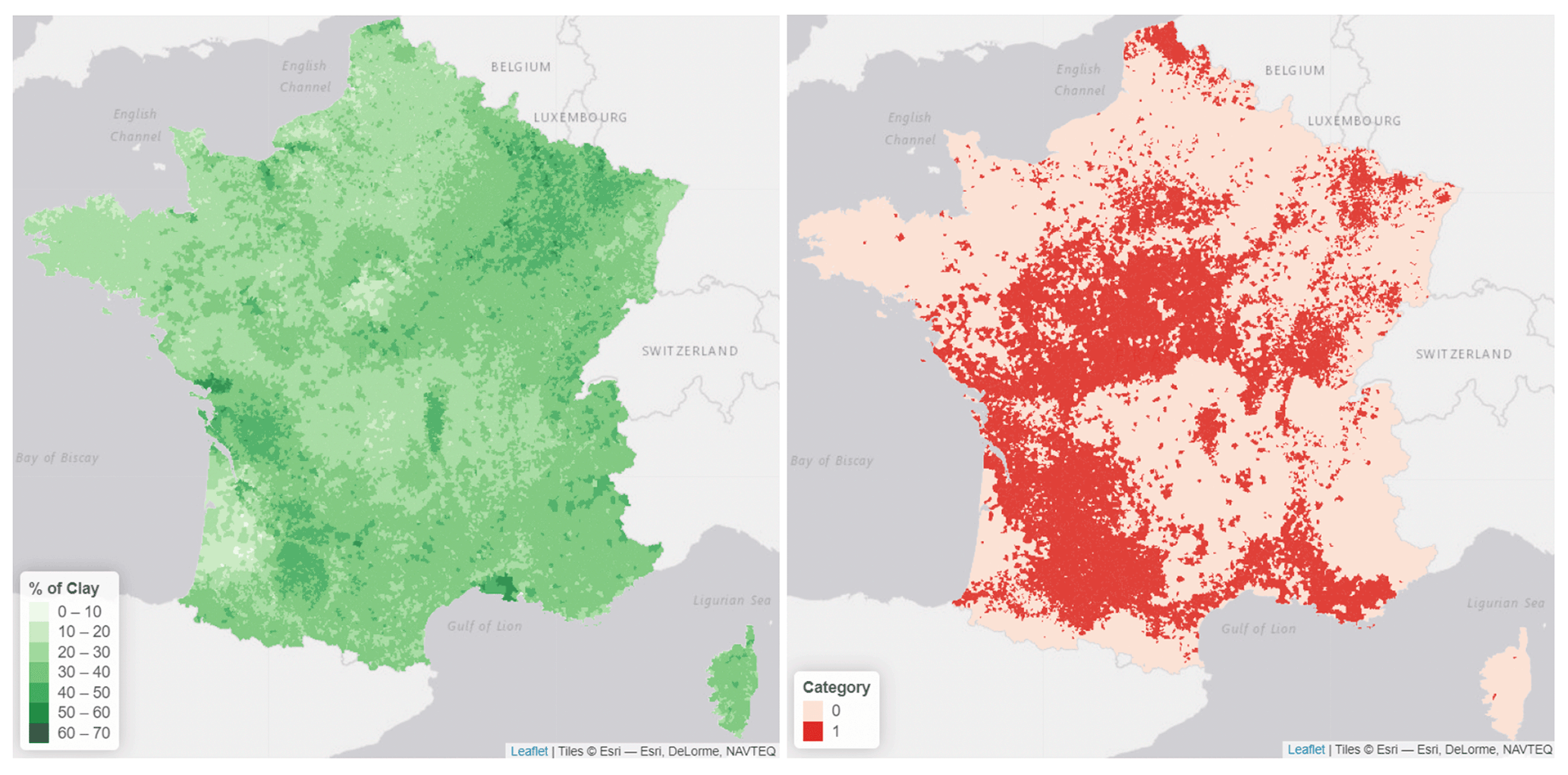
Figure 2Topsoil clay concentration (left) and historical natural catastrophes accepted requests (right). Those two variables will be used for our predictive model.
These variables were then aggregated to the exposure dataset. Thus, the calibration dataset was composed for each claim year of the INSEE code of the town (from the official classification, which can be seen as the equivalent of the ZIP code used in the USA), the year of the claim, the number of claims, the cost of claims (in EUR), the number of policies, the total sums insured (in EUR), the clay concentration in the soil, the ESPI, the ESSTI, the ESSWI and Cat (the binary categorical variable giving the occurrence of a historical natural catastrophe declaration request, prior to the year of study). All the models calibrated are based on those five variables mentioned above.
At a regional scale, Corti et al. (2009, 2011) pointed out that it is possible to use simulations to obtain a good representation of the regions affected by drought-induced soil subsidence, but substantial differences between simulated and observed damage in some regions remain. In this section, we will describe a simple spatio-temporal model for resilience to model either the frequency or the intensity of such events (on a yearly basis). Regression-type models will be considered as in Blauhut et al. (2016). The main difference is that the interest was to model occurrence, and a logistic regression was sufficient. Here, since we focus on frequency and intensity, some Poisson-type regression models will we considered first and then some gamma models for the severity, to predict the economic cost of subsidence. In Sect. 3.3 we will present regression-based models that we will extend in Sect. 3.4 to ensemble models, namely with bagging of regression trees, as suggested in Breiman (1996), to take into account some possible non-linearity as well as cross effects. And in Sect. 3.5, we will study more carefully the errors. But before this, we need to introduce some criteria to select an appropriate model.
3.1 Model selection criteria
Various validation performance measures are used to compare the different models. They are chosen to optimise the model selection based on the qualities that are desired from the model; i.e. they have a good capacity to predict the correct number of claims in the right areas and the ability to not predict claims where there are none historically, all the while keeping the simplest possible model. The following performance measures are thus used:
-
The Akaike information criterion (AIC) and Bayesian information criterion (BIC) were applied, which use maximum-likelihood and penalise models with too many variables and too many variables with respect to the number of observations respectively. These criteria are only used for the parametric regression models.
-
Root mean square error (RMSE) – or simply the sum of the squares of errors, which penalises greatly extreme errors, i.e. extreme deviations in predictions – is used. This will be used for costs and not counts.
3.2 Cross-validation method
In order to assess the predictive power of the calibrated models, cross-validation was used. The main goal of the models is to predict accurately the number of claims per town on a yearly basis; thus a yearly cross-validation that is derived from the basic cross-validation principle will be used.
The idea of cross-validation is related to in-sample against out-of-sample testing. In a nutshell, the model is fitted on a subset of the data, and validation is computed on observations that were left out. This approach is interesting to assess how the results of some statistical analysis will generalise to form an “independent” dataset. Note that it is possible to remove one single observation and to validate the model on that one observation – this is the “leave-one-out” approach – or to split the original dataset into k subgroups, to remove one subgroup to fit a model and make predictions based on that specific subgroup, and rotate – this is the “k-fold cross-validation” approach. In the case of spatio-temporal data, two approaches can be used:
-
Use some regions as subgroups, and then use a spatial k-fold approach (as in Pohjankukka et al., 2017) where the model is fitted on k−1 regions, and validation is based using a metric on the error in the region that was left out – it can be the sum of the squares of the difference or any metric discussed in the previous section.
-
Use cross-validation in time, but because of particular properties of the time dimension, cross-validation is performed by removing the future from the analysis (as in Bergmeir et al., 2018). At time t, we use observations up to time t to fit a model and then obtain a prediction for time t+1. In some sense, it is a classical leave-one-out procedure, except that we cannot use observations after time t+1 to obtain a prediction at time t+1. This approach is used in this study.
3.3 Regression-based models
A first attempt at modelling the yearly number of claims was made using generalised linear models (GLMs) with Poisson, binomial and negative-binomial distributions, which are the most adapted to the calibration data (based on counts). These models offer a simple and interpretable approach to modelling data by assuming that the response variable is generated by a given distribution and that its mean is linked to the q explanatory variables (where classically 𝒳=ℝq), through a link function. In this model, we have n spatial locations (the number of towns), T dates (the number of years), and q possible explanatory variables.
If we want to model the number of houses claiming a loss in a given location, the Poisson GLM is defined as , for a location z and a year t, where Ez,t is the exposure (the number of contracts in the town) and λz,t is the yearly intensity, per house:
where 's are features used for modelling, such as the ESSWI or the ESSTI. The prediction, performed at year based on a calibration set of years , is
and is based on estimator obtained on the training dataset with observations of years , using maximum-likelihood techniques, and
where geophysics covariates are known. In Table 1 several sets of parameter estimates are given (with t varying from 2008 until 2018).
Table 1Evolution of the parameters in the regression (Poisson regression). Numbers in brackets are the standard deviations of the parameters. Note that two ESPI parameters are not significant here (95% level).
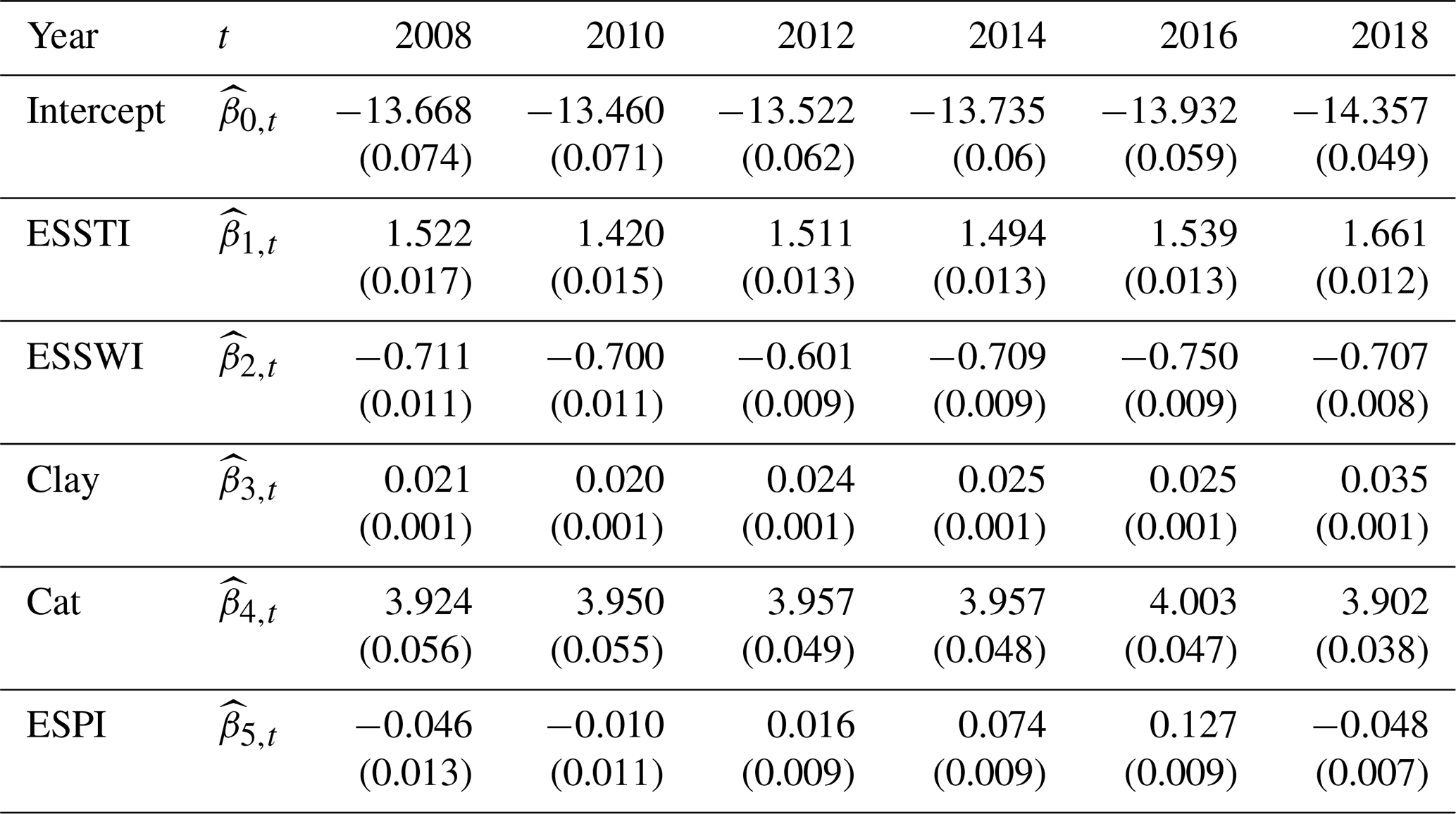
From Table 1, we can see that the model is rather stable over time, which is an interesting feature from a modeller's perspective: if we predict more claims due to subsidence in time, this is mainly due to the underlying factors than to the change in the impact of each variable. It can be mentioned that (associate with clay) is significantly increasing (with a p value of 2 %).
This Poisson model is rather classical for model counts, and it is said to be an equi-dispersed model, in the sense that the variance of Y is equal to the average value. This model can be extended in two directions.
-
First we have the binomial model, where , where Ez,t is the exposure and pz,t is the probability that, for a given year t and location z, a claim is made for a single house, and the prediction for is
In that case, we have an under-dispersed model in the sense that by construction we must have .
-
Second we have the negative-binomial (NB) model, where , in which Ez,t is the exposure and pz,t is the probability, with standard notations for the negative-binomial probability function. In that case, we have an over-dispersed model in the sense that .
Calibrating the GLMs and averaging the indicators over the years spanning from 2001 to 2018 and using the yearly cross-validation method, the results on the left of Table 2 were obtained. This table shows that the negative-binomial model has the lowest AIC and BIC.
In order to better consider the characteristics of the claim data, zero-inflated models were tested using Poisson and negative-binomial distributions. In these models the joint use of logistic and count regression allows the integration of the over-representation of non-events in the data. More formally, in zero-inflated models, given a location and a time (z,t), we assume that there is a probability of having zero claims. In our context, this could mean that the town has not been recognised as hit by a drought event. The occurrence of a drought is modelled with a logistic model with probability pz,t here. Then, if there is a drought event, the number of claims is driven by some specific distribution (Poisson, binomial or negative binomial), as introduced by Lambert (1992). If we consider a Poisson regression, this means that
(the second part comes from the fact there could be a drought, but the number of counts of claims is null) and
where and λz,t and pz,t are related to covariates through expressions as in Eqs. (4) and (7) respectively. Note that such models can easily be estimated with standard statistical packages. The results of the zero-inflated models are visible on the right of Table 2. It shows that the zero-inflated negative-binomial model is better than the zero-inflated Poisson model.

Figure 3 shows the yearly predictions for the zero-inflated models, alongside the previously tested GLMs.3
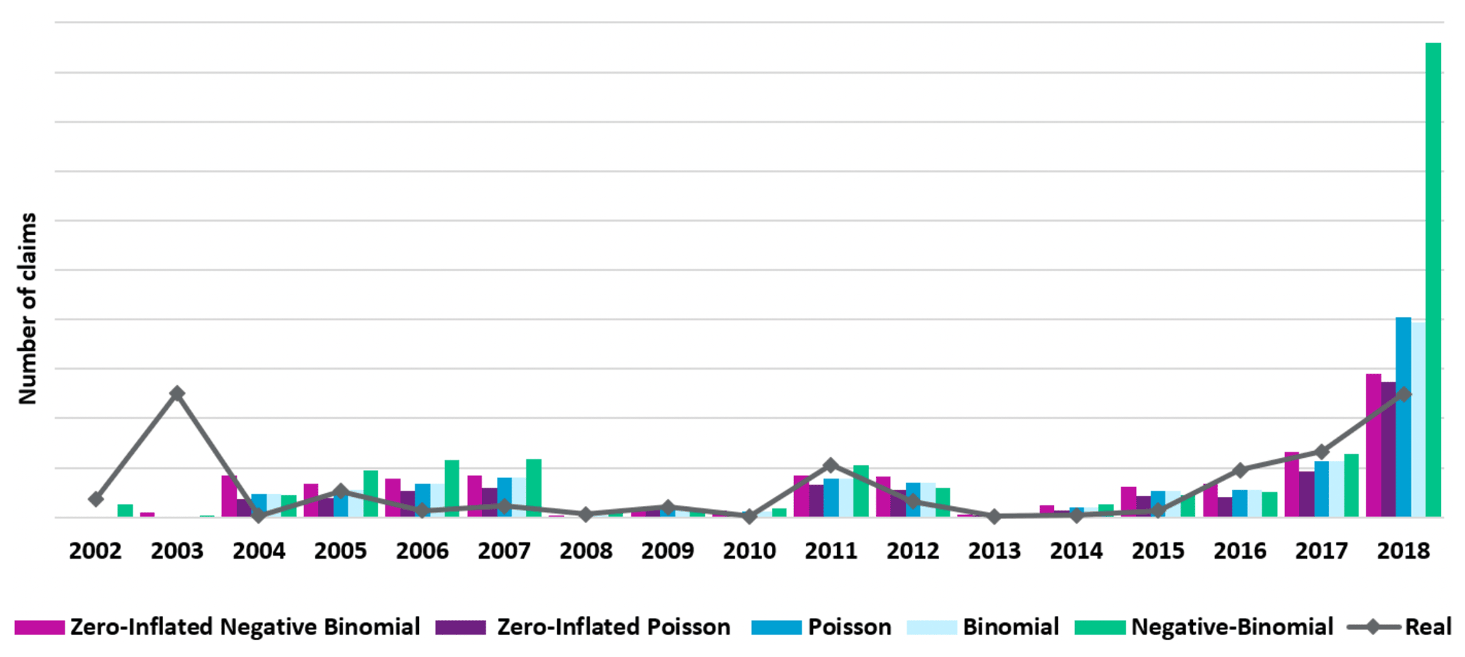
When looking at the yearly total predictions compared to reality, as observed in Fig. 3, all the GLM predictions are very similar apart from the negative-binomial model, which overpredicts (massively) in 2018; however they all overestimate claims in 2018 and underestimate the number of claims in 2003, 2011, 2016 and 2017. This graph shows that the predictions closest to the reality line are for the negative-binomial zero-inflated model. That model also has the best metrics when comparing them to those of the GLMs. Thus, zero-inflated models appear to provide a better fit than the GLMs.
This section showed that the zero-inflated models, in particular the negative-binomial zero-inflated model, outperformed the GLMs in terms of the number of claims and model selection criteria. In the next section, we will see the alternatives to regression-type models that can be considered since the “linear model” assumption might be rather strong here.
3.4 Tree-based models
Tree-based models are popular models for data analysis and prediction and offer an alternative to the previous parametric models. Popularised by Breiman et al. (1983), regression trees produce simple and easily interpretable split rules.
-
A regression tree is such that
where is a partition of 𝒳 and ℒj's are called leaves. In a tree with two leaves, {ℒ1,ℒ2}, there is a variable j such that ℒ1 is the half-space of 𝒳 characterised by while ℒ2 is characterised by for a threshold s. For the “classical” regression tree, the split is based on the squared loss function, in the sense that we select s to maximise the between variance or, equivalently, minimise the within variance. It is possible to extend this approach by using, instead of the squares of residuals (corresponding to the squared loss function), the opposite of the log likelihood of the data. This can be performed using the
rpartR package (see Breiman et al., 1983, for further details on regression trees).
If trees are simple to interpret, they are usually rather unstable: when fitting a tree on a subset of observations, it is common to obtain different splitting variables and therefore different trees. The idea of bagging (as defined in Breiman, 1996) is to use a bootstrap procedure to create samples (resampling the observations with replacement) and then aggregate predictions. In the case where the number of covariates is not too large, this is also called random forests, from Breiman (2001).
Two tree-based models are tested here in order to attempt to improve the previous predictions:
-
A classical random forest (RF),
is tested, where each tree – corresponding here to different i's – is computed using a squared loss function, on different bootstrap samples (obtained by resampling n observations, with replacement, out of the initial n ones). This can be performed using the
randomForestR package. -
A Poisson random forest (RFP) which considers count data, with the aim of better capturing the distribution of the data, is used. Poisson random forests are a modified version of Breiman's random forest, allowing the use of count data with different observation exposures. This is done by modifying the splitting criterion so that it maximises the decrease in the Poisson deviance. An offset has also been introduced to accommodate for different exposures. This random forest was calibrated using the
rfPoissonfunction available in therfCountDatapackage in R.
These random forests were all tuned in order to obtain the optimal number of trees, number of variables tested at each split and maximum number of nodes. However, the tuning was limited given the length of the tuning process, which may reduce the quality of the models.

Figure 4Comparison of yearly predictions for the tree-based models, with zero-inflated negative binomial (ZINB), classical RF and RFP.
Figure 4 shows the total yearly predictions for each tree-based model alongside the zero-inflated negative-binomial model and the real claims. It shows that the closest predictions to the real observations (the solid line) seem to be those of the zero-inflated model and the Poisson random forest, although all models but the zero-inflated model underestimate 2011 and 2016. With our cross-validation approach, we have poor results for early years (only data from 2002 were used to derive a model for 2003). The standard random forest overpredicts 2018. Thus, the zero-inflated model and the Poisson random forest appear to have the best predictions.
In this section, two different random forests were presented; however, the one with the best results is the Poisson random forest, which rendered similar results to the negative-binomial zero-inflated model. The complex calibration process and the unclear influence and importance of the variables on the output of the Poisson random forest make it a less attractive choice of model compared to the zero-inflated regression, which has a clear variable influence and a simple prediction formula. One can thus wonder whether such a loss in interpretability is worth such a small gain in terms of predictions.
3.5 Mapping the predictions
In order to improve the predictions and only predict the actually impacted areas, a methodology was developed to optimise the removal of all the very low claim predictions. This methodology was applied to both the zero-inflated model and the Poisson random forest. The total predictions changed little, and the geographical distribution of both models' predictions are observable for 2018 in Fig. 5.
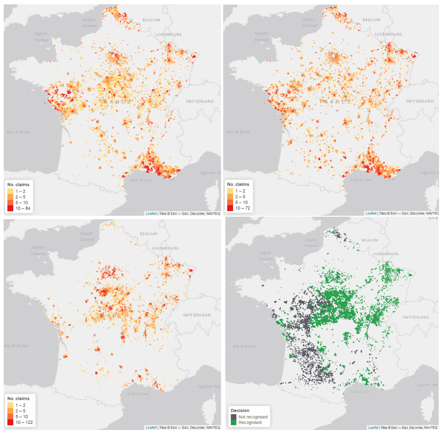
Figure 5Observed and predicted number of claims for 2018, with, from left to right, Poisson random forest and zero-inflated claims (on top) and observed claims and recognised ones (below).
In 2018, both models have more or less the same claim distribution, with large numbers of claims along the Mediterranean, in the north and in Pays de la Loire. However, the distribution is slightly different when looking at the centre of France. Indeed, the random forest seems to predict more claims in that area than the zero-inflated negative-binomial model. Comparing these results with the real claims for 2018, it can be seen that the historical claims are nearly exclusively concentrated in the centre of France with a few claims along the Atlantic and Mediterranean coast and in the north-east of France. Thus, both models seem to overpredict the claims around the coasts of France and – slightly for the Poisson random forest and vastly for the zero-inflated negative-binomial model – underpredict them in the centre of France. However, it can be noted that the overpredicted areas do mostly fall within areas that have non-recognised natural catastrophe declarations, which could mean that the area was hit but not compensated and thus that the models have difficulty assessing the difference between areas that will be recognised as natural catastrophes or not. The same conclusion can be made when looking at the predictions for 2017, visible in Fig. 6.
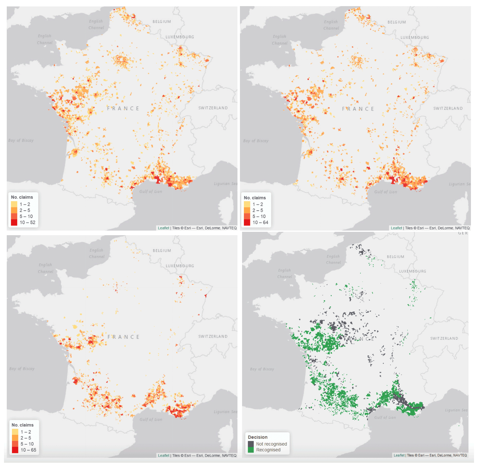
Figure 6Observed and predicted number of claims for 2017, with, from left to right, Poisson random forest and zero-inflated claims (on top) and observed claims and recognised ones (below).
In these maps, the predicted claims do appear to be in the correct areas in the south and south-west of France for both models; however, there are overpredictions in the east, centre and north of France, which also appear to be areas with non-accepted natural catastrophe declarations. Both models seem to predict not only the correct areas but also additional zones that often are areas that have had natural catastrophe declarations refused, which means that those areas were impacted by subsidence but not sufficiently to enter the scope of the natural catastrophe regime. Indeed, as the acceptance criteria changed frequently between 2001 and 2018, the models cannot capture the natural catastrophe aspect of a claim seeing as one that may have been acceptable in 2017 may no longer be today. Both models predict more or less the same geographical distribution of claims, posing the question of the usefulness and practicality of using a complex model such as the Poisson random forest compared to the zero-inflated negative-binomial model.
Another option that would permit the classification of the predicted claims into accepted and refused natural catastrophe categories would be to use the map of shrinkage and swelling of clay risk (Georisques, 2020), published by the French Geological Survey (BRGM). This map categorises the exposure of a given point of France using four categories: not at risk, low risk, average risk and high risk. The acceptance of a natural catastrophe declaration in France is feasible if more than 3 % of the surface of a town is in a zone with average or high risk. Thus, if the predicted claims map and the risk map, aggregated by town, were overlapped, the classification of the predicted claims would be possible between potentially accepted and most likely refused natural catastrophe declaration.
In the previous section, we saw different models used to predict frequency (the number of claims per town). Here we consider a gamma model for the average cost per claim, leading us towards a compound model for the total cost per town, as introduced in Adelson (1966) and used for example in hydrology in Revfeim (1984) or Svensson et al. (2017) or for droughts in Khaliq et al. (2011).
4.1 Modelling average and total economic costs
For a given location z and year t, the total cost (from the insurer's perspective) is a compound sum, in the sense that
with a random sum of random costs. Here Nz,t is the frequency, modelled in the previous section, and 's are individual economic losses per house. It is possible to consider here a Tweedie GLM, as introduced in Jørgensen (1997), corresponding to a compound Poisson model, with gamma average cost. Nevertheless this is only a subclass of the general compound models. Note that Tweedie models are related to a power parameter since they are characterised by the relationship 𝔼[Y]=Var[Y]γ. If γ=1, Y is proportional to a Poisson distribution (average costs are non-random), while γ=2 means that Y is proportional to a gamma distribution (frequency is non-random). For inference, we used γ=1.5, which corresponds to the lowest AIC. For the corresponding Tweedie model, the SSTI and SSWI, as well as clay and Cat covariates, were used.
Although the model is interesting, it is less flexible than having two separate models – one for the frequency and one for the average cost at location z, for year t, written
where (as before) Nz,t is the frequency, as modelled in the previous section, and the average cost (per house) is modelled using our data, aggregated at the town level, . The prediction is then
The results of these methods are rather similar. Figure 7 shows the total yearly predictions for the Tweedie model and the average-cost-of-claims method using the GLM and both the zero-inflated and the Poisson random forest models, previously calibrated.
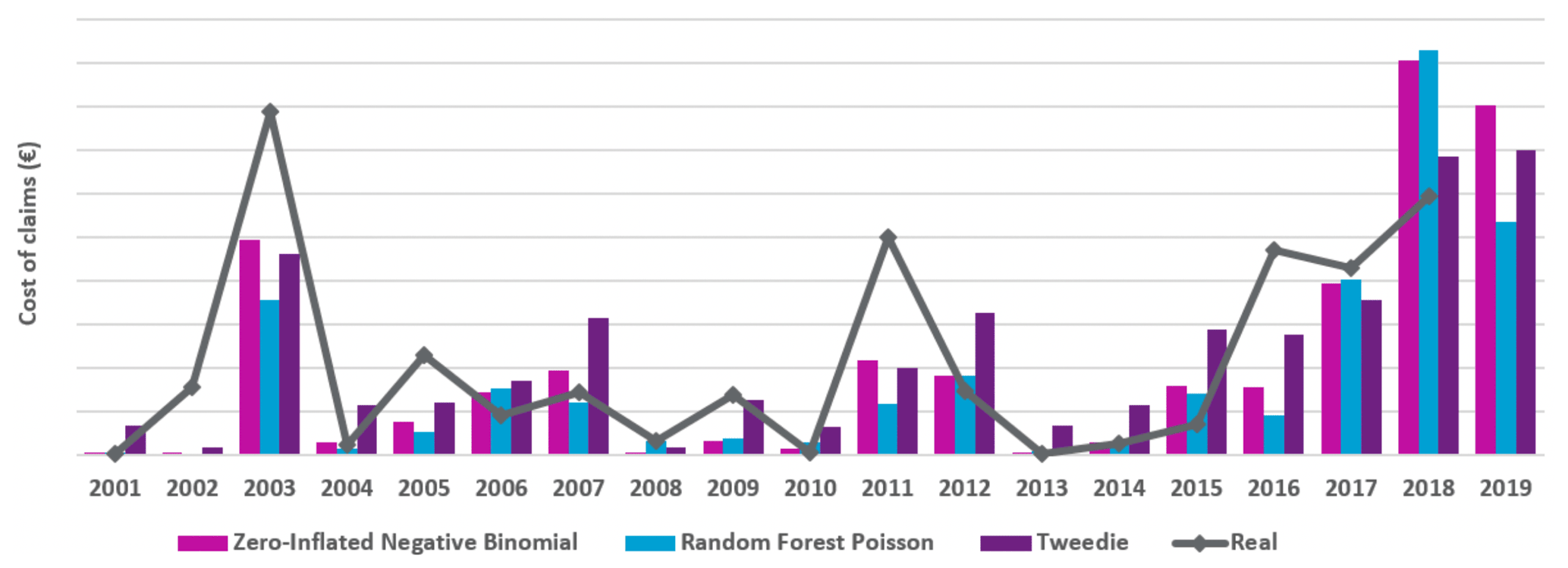
Figure 7Total yearly cost predictions in France, with a ZINB model + gamma costs, RFP model + gamma costs and a Tweedie model (Poisson + gamma costs).
Figure 7 shows that the Tweedie model makes predictions that are similar to the previous cost of claims predictions; however this model overestimates less in the year 2018 and (clearly) overestimates more in the years 2007 and 2012. On the other hand, the years 2003, 2011 and 2016 are still severely underestimated by the three predictions, although less so by the Tweedie model.
4.2 Mapping the predictions
As in Sect. 3.5, it is possible to visualise the prediction and to map and , as seen in Fig. 8. As expected, if we are not able to predict correctly the frequency, the cost is overestimated. Overall (as we can see in Fig. 7), in 2017, we obtained a good prediction in France, but we can observe some spatial differences. Most of the comments made in Sect. 3.5 remain valid, and clearly, predicting the economics losses in a specific area is not a simple task.
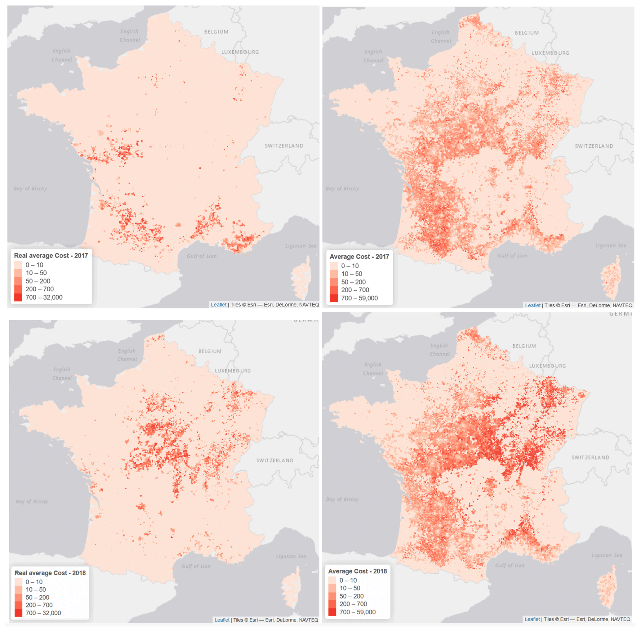
Figure 8Observed and predicted average cost of claims in 2017 (top). Observed and predicted average cost of claims in 2018 (bottom).
In this study, we considered forecasting claims for past data based on time t+1 up to time t and climatic variables for time t+1. Therefore, it is not possible to forecast claims in the future since we would have to obtain forecasts of future climate datasets for all three climatic indicators (ESSTI, ESSWI and ESPI) using the soil wetness, soil temperature and precipitation data in different RCP (Representative Concentration Pathway) scenarios and use these new future climate indicators to estimate the impact of climate change on future claims in each scenario. Furthermore, one must keep in mind that the results would be based on today's legal environment and would not take into account any evolution in the way subsidence claims are covered. This methodology would also be flawed by the generally larger granularity of future climate data, which renders the estimation less precise (e.g. CMIP5 future climate data (https://cds.climate.copernicus.eu/cdsapp#!/dataset/projections-cmip5-monthly-single-levels?tab=overview, last access: July 2020), which have lower resolution compared to ERA5-Land data used in this study).
The increase in the number and severity of subsidence claims in the past years has created a need for insurers to improve their grasp of the knowledge of this risk. However, the implementation of subsidence models is time-consuming and requires detailed data. This study proposed a method for approaching the costs and frequency of claims due to subsidence based on historical data. This was applied through two main components: the development of new drought indicators using open data and the use of parametric and tree-based models to model this risk. Modelling subsidence requires the integration of meteorological and geological indicators to ascertain the factors predisposing a policy to subsidence. Without this information, the inherent risk to which a dwelling is exposed cannot be perceived. For this reason, geological and meteorological data were obtained from open datasets. These data were paired with insurance exposure and claim data to obtain a complete dataset used to calibrate the models. However, the data available were only at a communal-mesh scale, making the results less precise. Indeed, subsidence is a very localised risk whose modelling would benefit from policy-level data.
Overall, the methods enable the predictions of an estimate of the number of claims, the cost of claims and their geographical distributions. Although they sometimes lack precision, the models give a good indication of the severity of a given year. The uncertainty in the predictions may be explained by the non-homogeneous data on which the models were calibrated. Indeed, the natural catastrophe declaration criteria evolved many times over the calibration period, rendering the historical data biased. The predictions would also have benefited from data at a finer mesh scale to take into account the individual particularities of each policy such as the presence of trees close to the construction, the slope of the terrain or the orientation of the slope. Finally, more precise temporal definition of the events could have been used if the claims were available at a monthly scale rather than yearly. In that case, seasonal indicators could have been created, rather than yearly ones, to capture more precisely the timescale of an event.
This study has allowed for the creation and implementation of new drought indicators for a subsidence claim model which performs well, considering the limitations induced by the lack of information and precision of the calibration dataset. The created model provides a better understanding of the phenomenon and allows other subsidence exposure evaluations to be challenged, which will improve an insurance company's management of this risk, given the lack of available subsidence models on the market. This methodology could be improved in the future by using policy-level data with a more accurate temporal definition of the claims in order to better apply the created indicators. The framework of this study is also in itself interesting and could be repurposed for other applications. Indeed, the studied models could be extended to other claim prediction problematics, for other types of peril for example, which are often confronted with similar issues of over-representation of non-recognised events.
Code is available at https://github.com/freakonometrics/subsidence/ (Charpentier, 2022a). The data used for the calibration in this study are based on datasets that are the property of private insurers in France and therefore cannot be shared; however a sample of the data will be provided in the Zenodo project folder (https://doi.org/10.5281/zenodo.6863730, Charpentier, 2022b).
HA provided insurance data and provided technical support. MJ developed the model code and performed the simulations. AC prepared the manuscript with contributions from the other co-authors.
The contact author has declared that none of the authors has any competing interests.
Publisher’s note: Copernicus Publications remains neutral with regard to jurisdictional claims in published maps and institutional affiliations.
This article is part of the special issue “Drought vulnerability, risk, and impact assessments: bridging the science-policy gap”. It is not associated with a conference.
The authors wish to thank Hélène Gibello, Sonia Guelou, Florence Picard and Franck Vermet for comments on a previous version of the work. Arthur Charpentier received financial support from the Natural Sciences and Engineering Research Council of Canada (NSERC-2019-07077) and the AXA Research Fund.
This research has been supported by the Natural Sciences and Engineering Research Council of Canada (grant no. NSERC-2019-07077) and the AXA Research Fund (JRI Unusual Data for Insurance).
This paper was edited by Joaquim G. Pinto and reviewed by Sien Kok and one anonymous referee.
Adelson, R. M.: Compound poisson distributions, J. Oper. Res. Soc., 17, 73–75, 1966. a
Antoni, V., Janvier, F., and Albizzati, C.: Retrait-gonflement des argiles: plus de 4 millions de maisons potentiellement très exposées, Commissariat général au développement durable, 122, https://notre-environnement.gouv.fr/rapport-sur-l-etat-de-l-environnement/themes-ree/risques-nuisances-pollutions/risques-naturels/autres-risques-naturels/article/le-retrait-gonflement-des-argiles (last access: July 2022), 2017. a
Association Française de l'Assurance (AFA): Risques climatiques: quel impact sur l'assurance contre les aléas naturels à l'horizon 2040?, https://www.franceassureurs.fr/wp-content/uploads/VF_France-Assureurs_Impact-du-changement-climatique-2050.pdf (last access: July 2022), 2015. a
Bergmeir, C., Hyndman, R. J., and Koo, B.: A note on the validity of cross-validation for evaluating autoregressive time series prediction, Comput. Stat. Data An., 120, 70–83, 2018. a
Bevere, L. and Weigel, A.: Exploring the secondary perils universe, Order no. 270_0121_EN, Swiss Re Sigma, https://www.swissre.com/dam/jcr:ebd39a3b-dc55-4b34-9246-6dd8e5715c8b/sigma-1-2021-en.pdf (last access: July 2020), 2021. a, b
Bidan, P. and Cohignac, T.: Le régime francais des catastrophes naturelles: historique du régime, Variances, 11, https://variances.eu/?p=2705 (last access: July 2020), 2017. a
Blauhut, V., Stahl, K., Stagge, J. H., Tallaksen, L. M., De Stefano, L., and Vogt, J.: Estimating drought risk across Europe from reported drought impacts, drought indices, and vulnerability factors, Hydrol. Earth Syst. Sci., 20, 2779–2800, https://doi.org/10.5194/hess-20-2779-2016, 2016. a
Bradford, R.: Drought events in europe, in: Drought and drought mitigation in Europe, edited by: Vogt, J. V. and Somma, F., 7–20, Springer, Dordrecht, https://doi.org/10.1007/978-94-015-9472-1_2, 2000. a
Breiman, L.: Bagging predictors, Mach. Learn., 24, 123–140, 1996. a, b
Breiman, L.: Random forests, Mach. Learn., 45, 5–32, 2001. a
Breiman, L., Friedman, J. H., Olshen, R. A., and Stone, C. J.: Classification and regression trees, 1st Edn., Routledge. https://doi.org/10.1201/9781315139470, 1983. a, b
Brignall, A. P., Gawith, M. J., Orr, J. L., and Harrison, P. A.: Assessing the potential effects of climate change on clay shrinkage-induced land subsidence, in: Climate, Change and Risk, 84–102, Routledge, ISBN 9780203026175, 2002. a
Bucheli, J., Dalhaus, T., and Finger, R.: The optimal drought index for designing weather index insurance, Eur. Rev. Agric. Econ., 48, 573–597, 2021. a
Caisse Centrale de Réassurance: Les Catastrophe Naturelles en France: Bilan 1982–2020, https://side.developpement-durable.gouv.fr/ACCIDR/doc/SYRACUSE/795441 (last access: July 2022), 2019. a
Caisse Centrale de Réassurance: Arrêtés de catastrophes naturelles, http://catastrophes-naturelles.ccr.fr/les-arretes (last access: June 2022), 2020. a
Charpentier, A.: Insurability of climate risks, The Geneva Papers on Risk and Insurance-Issues and Practice, 33, 91–109, 2008. a
Charpentier, A.: Code to “Predicting drought and subsidence risks in France”, GitHub [code], https://github.com/freakonometrics/subsidence/, last access: 19 July 2022a. a
Charpentier, A.: freakonometrics/subsidence: subsidence (v1.0.1), Zenodo [data set, code], https://doi.org/10.5281/zenodo.6863730, 2022b. a
Charpentier, A., Barry, L., and James, M.: Insurance against natural catastrophes: balancing actuarial fairness and social solidarity, Geneva Pap. R. I.-Iss. P., 47, 50–78, https://doi.org/10.1057/s41288-021-00233-7, 2022. a, b
Climate Change Service Climate Data Store (CDS): Copernicus climate change service (c3s) (2017): Era5: Fifth generation of ecmwf atmospheric reanalyses of the global climate, https://cds.climate.copernicus.eu/cdsapp#!/home (last access: July 2022), 2020. a
Corti, T., Muccione, V., Köllner-Heck, P., Bresch, D., and Seneviratne, S. I.: Simulating past droughts and associated building damages in France, Hydrol. Earth Syst. Sci., 13, 1739–1747, https://doi.org/10.5194/hess-13-1739-2009, 2009. a, b
Corti, T., Wüest, M., Bresch, D., and Seneviratne, S. I.: Drought-induced building damages from simulations at regional scale, Nat. Hazards Earth Syst. Sci., 11, 3335–3342, https://doi.org/10.5194/nhess-11-3335-2011, 2011. a
Doornkamp, J. C.: Clay shrinkage induced subsidence, Geogr. J., 159, 196–202, 1993. a
Entidad Estatal de Seguros Agrarios (ENESA): La sequía, un riesgo incluido en los seguros agrarios, Noticias Del Seguro, 82, 3–5, 2012. a
European Soil Data Centre (ESDAC): Topsoil physical properties for europe (based on lucas topsoil data), https://esdac.jrc.ec.europa.eu (last access: July 2022), 2015. a
Farahmand, A. and AghaKouchak, A.: A generalized framework for deriving nonparametric standardized drought indicators, Adv. Water Resour., 76, 140–145, 2015. a
Frécon, J. and Keller, F.: Sécheresse de 2003: un passé qui ne passe pas, rapport d'information fait au nom du groupe de travail sur la situation des sinistrés de la sécheresse de 2003 et le régime d'indemnisation des catastrophes naturelles constitué par la commission des finances, French Senate Technical Report, 39, https://www.senat.fr/notice-rapport/2009/r09-039-notice.html (last access: July 2022), 2009. a
Georisques: Gestion assistée des procédures administratives relatives aux risques, https://www.georisques.gouv.fr/donnees/bases-de-donnees/base-gaspar (last access: July 2022), 2020. a
Gourdier, S. and Plat, E.: Impact of climate change on claims due to the shrinkage and swelling of clay soils, Journées Nationales de Géotechnique et de Géologie de l'Ingénieur, 1–8, https://hal-brgm.archives-ouvertes.fr/hal-01768395 (last access: July 2022), 2018. a
Guttman, N. B.: Comparing the palmer drought index and the standardized precipitation index, J. Am. Water Resour. As., 34, 113–121, 1998. a
Hagenlocher, M., Meza, I., Anderson, C. C., Min, A., Renaud, F. G., Walz, Y., Siebert, S., and Sebesvari, Z.: Drought vulnerability and risk assessments: state of the art, persistent gaps, and research agenda, Environ. Res. Lett., 14, 083002, https://doi.org/10.1088/1748-9326/ab225d, 2019. a, b
Hao, Z. and AghaKouchak, A.: A nonparametric multivariate multi-index drought monitoring framework, J. Hydrometeorol., 15, 89–101, 2014. a
Herrera-García, G., Ezquerro, P., Tomás, R., Béjar-Pizarro, M., López-Vinielles, J., Rossi, M., Mateos, R. M., Carreón-Freyre, D., Lambert, J., Teatini, P., Cabral-Cano, E., Erkens, G., Galloway, D., Hung, W.-C., Kakar, N., Sneed, M., Tosi, L., Wang, H., and Ye, S.: Mapping the global threat of land subsidence, Science, 371, 34–36, 2021. a
Iglesias, A., Assimacopoulos, D., and van Lanen, H. (Eds.): Drought: Science And Policy, Wiley-Blackwell, ISBN 978-1-119-01707-3, 2019. a, b
Ionita, M. and Nagavciuc, V.: Changes in drought features at the European level over the last 120 years, Nat. Hazards Earth Syst. Sci., 21, 1685–1701, https://doi.org/10.5194/nhess-21-1685-2021, 2021. a
Jørgensen, B.: The Theory of Dispersion Models, Chapman & Hall, ISBN 978-0412997112, 1997. a
Kchouk, S., Melsen, L. A., Walker, D. W., and van Oel, P. R.: A geography of drought indices: mismatch between indicators of drought and its impacts on water and food securities, Nat. Hazards Earth Syst. Sci., 22, 323–344, https://doi.org/10.5194/nhess-22-323-2022, 2022. a
Khaliq, M. N., Ouarda, T. B. M. J., Gachon, P., and Sushama, L.: Stochastic modeling of hot weather spells and their characteristics, Clim. Res., 47, 187–199, 2011. a
Kok, S. and Costa, A.: Framework for economic cost assessment of land subsidence, Nat. Hazards, 106, 1931–1949, 2021. a
Lambert, D.: Zero-inflated poisson regression, with an application to defects in manufacturing, Technometrics, 34, 1–14, 1992. a
Lloyd-Hughes, B. and Saunders, M. A.: A drought climatology for europe, Int. J. Climatol., 22, 1571–1592, 2002. a
Magnan, S.: Catastrophe insurance system in france, Geneva Papers on Risk and Insurance, Issues and Practice, 474–480, https://doi.org/10.1057/gpp.1995.42, 1995. a
McCullough, K. A.: Managing subsidence, Journal of Insurance Issues, 27, 1–21, 2004. a, b
McKee, T. B., Doesken, N. J., and Kleist, J.: The relationship of drought frequency and duration to time scales, Eighth Conference on Applied Climatology, https://www.droughtmanagement.info/literature/AMS_Relationship_Drought_Frequency_Duration_Time_Scales_1993.pdf (last access: July 2022), 1993. a
Mills, E.: Synergisms between climate change mitigation and adaptation: an insurance perspective, Mitig. Adapt. Strat. Gl., 12, 809–842, 2007. a
Ministère de la transition écologique et solidaire (MTES): Le retrait-gonflement des argiles: Comment prévenir les désordres dans l'habitat individuel, https://www.ecologie.gouv.fr/sites/default/files/dppr_secheresse_v5tbd.pdf (last access: July 2022), 2016. a, b, c
Ministère de l'intérieur (MI): Procédure de reconnaissance de l'état de catastrophe naturelle – révision des critères permettant de caractériser l'intensité des épisodes de sécheresses-réhydrations des sols a l'origine des mouvement de terrains différentiels, Technical report, NOR: INTE1911312C, https://www.legifrance.gouv.fr/download/pdf/circ?id=44648 (last access: July 2022), 2019. a, b
Mission des Risques Naturels (MRN): Lettre d'information de la mission des risques naturels, 07, Lettre, no. 30, July 2019, https://www.mrn.asso.fr/wp-content/uploads/2019/10/lettre-n30_vf.pdf (last access: July 2022), 2019. a
Mission des Risques Naturels (MRN): Bilan des principaux évènements cat-clim, Lettre d'information, 35, https://www.mrn.asso.fr/wp-content/uploads/2021/02/lettre-n35_vf.pdf (last access: July 2022), 2021. a
Naumann, G., Spinoni, J., Vogt, J. V., and Barbosa, P.: Assessment of drought damages and their uncertainties in europe, Environ. Res. Lett., 10, 124013, https://doi.org/10.1038/s41558-021-01044-3, 2015. a
Naumann, G., Cammalleri, C., Mentaschi, L., and Feyen, L.: Increased economic drought impacts in europe with anthropogenic warming, Nat. Clim. Change, 11, 485–491, 2021. a
Pérez-Blanco, C. D., Delacámara, G., Gómez, C. M., and Eslamian, S.: Crop insurance in drought conditions, in: Handbook of Drought and Water Scarcity, Vol. 1, 423–444, CRC Press, ISBN 9781315226781, 2017. a
Pohjankukka, J., Pahikkala, T., Nevalainen, P., and Heikkonen, J.: Estimating the prediction performance of spatial models via spatial k-fold cross validation, Int. J. Geogr. Inf. Sci., 31, 2001–2019, 2017. a
Revfeim, K.: An initial model of the relationship between rainfall events and daily rainfalls, J. Hydrol., 75, 357–364, 1984. a
Schwarze, R., Schwindt, M., Weck-Hannemann, H., Raschky, P., Zahn, F., and Wagner, G. G.: Natural hazard insurance in europe: tailored responses to climate change are needed, Environ. Policy Gov., 21, 14–30, 2011. a
Soubeyroux, J.-M., Vidal, J.-P., Najac, J., Kitova, N., Blanchard, M., Dandin, P., Martin, E., Pagé, C., and Habets, F.: Projet climsec: Impact du changement climatique en france sur la sécheresse et l'eau du sol, Hal-archive, 00778604, 9–16, https://hal.inrae.fr/view/index/identifiant/hal-00778604 (last access: July 2022), 2011. a
Soubeyroux, J.-M., Kitova, N., Blanchard, M., Vidal, J.-P., Martin, E., and Dandin, P.: Caractérisation des sècheresses des sols en France et changement climatique: Résultats et applications du projet ClimSec, La Météorologie, 78, 21–30, 2012. a, b
Soyka, T.: A crack in the wall of your home: it could be subsidence, an almost invisible natural hazard, Swiss Re., https://www.swissre.com/risk-knowledge/mitigating-climate-risk/crack-in-the-wall-of-your-home.html (last access: July 2022), 2021. a
Spinoni, J., Naumann, G., Carrao, H., Barbosa, P., and Vogt, J.: World drought frequency, duration, and severity for 1951–2010, Int. J. Climatol., 34, 2792–2804, 2014. a
Spinoni, J., Naumann, G., Vogt, J., and Barbosa, P.: European drought climatologies and trends based on a multi-indicator approach, Global Planet. Change, 127, 50–57, 2015. a
Spinoni, J., Naumann, G., and Vogt, J. V.: Pan-european seasonal trends and recent changes of drought frequency and severity, Global Planet. Change, 148, 113–130, 2017. a
Svensson, C., Hannaford, J., and Prosdocimi, I.: Statistical distributions for monthly aggregations of precipitation and streamflow in drought indicator applications, Water Resour. Res., 53, 999–1018, 2017. a
Svoboda, M. and Fuchs, B.: World Meteorological Organization (WMO) and Global Water Partnership (GWP), 2016: Handbook of Drought Indicators and Indices, Integrated Drought Management Programme (IDMP), Integrated Drought Management Tools and Guidelines Series 2, Geneva, ISBN 978-92-63-11173-9, 2016. a, b
Torelló-Sentelles, H. and Franzke, C. L. E.: Drought impact links to meteorological drought indicators and predictability in Spain, Hydrol. Earth Syst. Sci., 26, 1821–1844, https://doi.org/10.5194/hess-26-1821-2022, 2022. a
Tsegai, D. and Kaushik, I.: Drought risk insurance and sustainable land management: what are the options for integration?, in: Current Directions in Water Scarcity Research, Vol. 2, 195–210, Elsevier, 2019. a
Vroege, W., Dalhaus, T., and Finger, R.: Index insurances for grasslands – a review for europe and north-america, Agr. Syst., 168, 101–111, 2019. a
Wües, M., Bresch, D., and Corti, T.: The hidden risks of climate change: An increase in property damage from soil subsidence in europe, Swiss Re., https://www.preventionweb.net/files/20623_soilsubsidencepublicationfinalen1.pdf (last access: July 2022), 2011. a, b
Here, we use here the word “town” to designate a “commune” (in French) or “municipality”. There are 37 613 towns in metropolitan France (as characterised by their INSEE commune code).
Here, we use either the minimum or the maximum, depending on whether drought events are related to either low or high values of seasonal indexes.
For purposes of confidentiality, the total number of claims per year is withheld, but the proportions on the y axis are valid.