the Creative Commons Attribution 4.0 License.
the Creative Commons Attribution 4.0 License.
 | 18 Jul 2022
Storm surge hazard over Bengal delta: a probabilistic–deterministic modelling approach
Md Jamal Uddin Khan
Fabien Durand
Kerry Emanuel
Yann Krien
Laurent Testut
A. K. M. Saiful Islam
Storm-surge-induced coastal inundation constitutes a substantial threat to lives and properties along the vast coastline of the Bengal delta. Some of the deadliest cyclones in history made landfall in the Bengal delta region claiming more than half a million lives over the last five decades. Complex hydrodynamics and observational constraints have hindered the understanding of the risk of storm surge flooding of this low-lying (less than 5 m above mean sea level), densely populated (> 150 million) mega-delta. Here, we generated and analysed a storm surge database derived from a large ensemble of 3600 statistically and physically consistent synthetic storm events and a high-resolution storm surge modelling system. The storm surge modelling system is developed based on a custom high-accuracy regional bathymetry enabling us to estimate the surges with high confidence. From the storm surge dataset, we performed a robust probabilistic estimate of the storm surge extremes. Our ensemble estimate shows that there is a diverse range of water level extremes along the coast and the estuaries of the Bengal delta, with well-defined regional patterns. We confirm that the risk of inland storm surge flooding at a given return period is firmly controlled by the presence of coastal embankments and their height. We also conclude that about 10 % of the coastal population is living under the exposure of a 50-year return period inundation under current climate scenarios. In the face of ongoing climate change, which is likely to worsen the future storm surge hazard, we expect our flood maps to provide relevant information for coastal infrastructure engineering, risk zoning, resource allocation, and future research planning.
- Article
(3425 KB) - Full-text XML
-
Supplement
(3059 KB) - BibTeX
- EndNote


Among global coastlines exposed to storm surges, the countries along the Indian Ocean have some of the places most severely impacted by deadly cyclones (Needham et al., 2015). Particularly the northern Bay of Bengal is one of the deadliest regions in terms of cyclone-related mortality (Ali, 1999). Although a tiny percentage (∼ 6 %) of cyclones form and make landfall around this region, the total death toll is more than 50 % of the global total (Alam and Dominey-Howes, 2014). The Bay of Bengal experiences, on average, five surge events per decade, exceeding a surge level (excess water level above the tidal prediction) of 5 m (Needham et al., 2015). The Bengal delta coastline, located in the northern Bay of Bengal spanning Bangladesh and India, experiences a large portion of the aforementioned cyclonic storms and associated storm surges. More than 100 million people live below 10 m elevation in this densely populated mega-delta region (Becker et al., 2019). Unsurprisingly, in the Bengal delta region, higher surge levels have a statistically significant correlation with the number of casualties in the past cyclones (Seo and Bakkensen, 2017).
Figure 1 illustrates a representative subset of the deadly cyclones that occurred in the last five decades. Table 1 lists the illustrated subset of cyclones and associated maximum water levels. This list is not exhaustive and is only shown here to illustrate the storm surge hazard. For a comprehensive historical catalogue of cyclones over the Bengal delta region, see Alam and Dominey-Howes (2014).
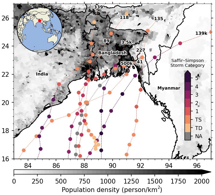
Figure 1Population density in the Bengal delta covering Bangladesh and India. A subset of cyclone tracks that made landfall in past decades is displayed as dashed lines. Inset shows the location of the study area. The colour-coded lines show the cyclone strength along its track on the Saffir–Simpson scale. TD and TS correspond to tropical depression and tropical storm, respectively. For the 1970 Bhola cyclone, the wind speed is not available (NA) and is shown in grey. The associated number at the head of the cyclone tracks refers to the number of casualties.
This small sample of cyclones and their associated surge indicate that cyclones can induce strong storm surges along this macro-tidal region of the world, depending on the tidal condition on their landfall. The regional characteristics of the tide are predominantly semi-diurnal in this region (Sindhu and Unnikrishnan, 2013). The tidal range is high, reaching about 5 m along the north-east coast (Krien et al., 2016; Khan et al., 2020). Additionally, a sizable continental river flow discharges through the distributaries of Ganges–Brahmaputra–Meghna (Mohammed et al., 2018). The shallow coastal submarine delta with an average width of 50 km provides favourable conditions for the development of large surges and strong interactions with tides (Krien et al., 2017b). The combination of all the aforementioned properties can give rise to high storm-driven water levels that have the potential to inundate the low-lying delta region and to cause thousands of casualties (Murty et al., 1986). Considering the tidal range and strong tide–surge interaction, the term “water level” is hereafter used to refer to the water level derived from the dynamic interaction of tide, surges, and waves.
Although we have opened our problem statement highlighting the deadliness of the cyclones making landfall in the Bengal delta region, the number of casualties from the storm surge has been reduced drastically over the last decades (Paul, 2009). This improvement is partly due to the governmental effort to build cyclone shelters and pre-storm preparedness. The local government and communities put substantial efforts to implement timely evacuations during storms. Continued development in the communications system (e.g. mobile phone network) and improvement in the numerical storm and surge forecasting further facilitated the evacuation effort. Engineering structures like embankments, which were built to promote agriculture through controlling tidal flooding (Nowreen et al., 2013), also provided a significant level of protection during storm surge events (Adnan et al., 2019). For a recent storm, supercyclone Amphan, Khan et al. (2021a) show that the major mode of flooding was due to failure of the dikes, indicating either inadequate design, poor maintenance, or both. Confident engineering design and continued maintenance of these structures, however, depends on the understanding of the variability in sea level, particularly the extreme water levels (Chowdhury et al., 1998).
Unfortunately, the variability in water level along the intricate coastline of the Bengal delta is poorly observed (Woodworth et al., 2016). The available limited set of water level observations reveals regionally varying water level dynamics at long, as well as short, timescales (Tazkia et al., 2017; Becker et al., 2020; Antony et al., 2016). For instance, Antony et al. (2016) found a robust amplification of extreme high water levels from south to north along the east coast of India. In their analysis, the tide appears as the largest contributor to extreme high-water events. At seasonal timescale, Tazkia et al. (2017) showed a summer–winter variability in mean sea level along the Bengal delta coastlines reaching up to 70 cm in range. At decadal scale, Becker et al. (2020) showed a consistent increase in relative sea level over the delta from an extensive database of daily water level records.
Nevertheless, due to the limited availability of water level records, consistent estimation of water level hazard for storm surge from in situ observations is not yet realized in this region (Lee, 2013; Chiu and Small, 2016). The main challenge is to secure hourly (or higher temporal resolution) tide gauge records that are long enough for reliable statistical analysis (Unnikrishnan and Sundar, 2004). The separation of short timescale (driven by meteorological effects, among which surges) from longer timescale (driven by tidal effects) on water level variability poses another challenge. The failure of tide gauges during a cyclonic event is also commonplace, causing bias in the record of extreme water levels (Antony et al., 2016; Krien et al., 2017b; Chiu and Small, 2016).
Hydrodynamic modelling of the storm surges has been used, with varying degrees of complexity, to curb the aforementioned data unavailability problems – along both the east coast of India (Chittibabu et al., 2004; Jain et al., 2010; Sindhu and Unnikrishnan, 2011) and the coast of Bangladesh (Chowdhury et al., 1998; Jakobsen et al., 2006).
Along the east coast of India, the approaches taken by Chittibabu et al. (2004) and that of Jain et al. (2010) are similar. Their estimation of the 50-year return period water level involved determining a 50-year return level of the atmospheric pressure drop (ΔP) from the observed cyclone records. Afterwards, they used the pressure drop estimate in conjunction with artificial cyclone tracks to spatially cover the area of interest. In their approach, the tide is added linearly to the cyclone surge. For example, Chittibabu et al. (2004) estimated the 50-year return period tidal water level and added it with the 50-year surge water level. On the other hand, Jain et al. (2010) added the total tidal amplitude for M2, S2, and K1 from the FES2004 global tidal atlas (Lyard et al., 2006) to the estimated surge water level. Both studies considered an additional constant water level of 50 cm to account for the wave set-up. This approach by Chittibabu et al. (2004) and Jain et al. (2010) assumes that tide and surge do not have any interdependence and that the 50-year return level tide and 50-year return level surge add up to a 50-year return level tide–surge. Moreover, the wave set-up is assumed to be the same for all return periods in the sense that the linear addition of the wave set-up does not change the return period of an estimated water level. For the Orissa coast in India (19∘ N–21∘ N), they both obtained a similar pattern of combined total water level (combining surge, tide, and wave set-up) at a 50-year return period with an increase from 4.3 m in the south to 8.5 m in the north. The numbers reported in Jain et al. (2010) (see their Fig. 10) seem to be the same as those of Chittibabu et al. (2004) (see their Fig. 8b). Along the coastline of West Bengal (21∘ N–20∘ N), the estimated 50-year return level ranges from 5 to 10 m.
Sindhu and Unnikrishnan (2011) addressed the non-linear dependence of tide and surge with a coupled tide–surge model. In their analysis, Sindhu and Unnikrishnan (2011) simulated 136 events spanning 1974 to 2000 to estimate maximum water levels during those storms. They applied an extreme value analysis on the estimated water levels using an r largest annual maximum approach to determine the return period of extreme water levels. Similar to Chittibabu et al. (2004) and Jain et al. (2010), Sindhu and Unnikrishnan (2011) also found an increasing amplitude of the 50-year return level of total sea level from south to north along the east coast of India. The highest 50-year return period water level was estimated in the northern edge – Sagar Island (21.72∘ N, 88.11∘ E) (8.7 m) and Chandipur (21.43∘ N, 87.01∘ E) (6.9 m). Compared to the 50-year return water level estimates of Chittibabu et al. (2004) and Jain et al. (2010), the estimates by Sindhu and Unnikrishnan (2011) are inferior in water level by about 50 % throughout the coast of Orissa. One notable issue with the approach of Sindhu and Unnikrishnan (2011) is, however, the limited number of available storm events. They derived the extreme water level along the 1200 km shoreline from 136 storm events, i.e. three events per 30 km (typical footprint of storm surges). This spatial sampling is potentially not adequate to capture the storm surge water level at various phases of the tide. Additionally, the storm parameters – notably maximum wind speed, radius of maximum wind, and central pressure – are collected over a long period, and the homogeneity of the storm records is not well defined (Singh et al., 2020). Finally, these studies focusing on the east coast of India do not cover the Bangladesh part of the delta, where a larger tide and a stronger tide–surge interaction are observed (Antony and Unnikrishnan, 2013).
In the Bangladesh part of the delta, Chowdhury et al. (1998) estimated the water levels inside the estuaries with a one-dimensional model at a 10- to 50-year return period to plan the construction of cyclone shelters. In their approach, they used an empirical formulation to estimate the surge level for a given wind speed. To estimate the surge level at a given return period, they assumed that the surge height corresponds to the wind speed of the approaching cyclone to that location at half the return period. This relatively simple approximate solution holds on this macro-tidal regime. Statistically, the tidal water level is relatively high for about half of the cyclones – those making landfall during the high-tide part of the tidal cycle. Their estimated 50-year return period surge level ranges from 3 to 4 m along the central part of the delta from west to east. However, in the final estimate for the design water level for the cyclone shelters in their study, they added the spring tide level linearly. They did not, however, provide an estimate of the total water level at the 50-year return period.
Jakobsen et al. (2006) took an approach similar to Sindhu and Unnikrishnan (2011) to estimate the extreme water level. For the Bengal delta coastline (of about 300 km length) they selected 17 historic cyclones that produced significant surges during 1960–2000. The simulated 17 water level records at each model grid point were then fitted to an exponential distribution to estimate the associated distribution parameters. According to their estimate, the 100-year return period water level goes as high as 10 m at the north-eastern corner of the estuary. They also noted a rapid evolution of water level with return periods along the shoreline of the lower part of the Meghna estuary.
From the literature review, it is clear that the unavailability of data also hindered the previous attempts to map the storm surge hazard using numerical models. This lack of data includes both the storm track records and associated storm parameters – e.g. pressure drop (ΔP), maximum wind speed (Vmax), and radius of maximum wind (Rm). The recorded storm parameters also have inherent inhomogeneity due to gradual changes in observational techniques (Singh et al., 2020). Finally, the spatial and temporal coverage of the recorded storms is sparse relative to the size of the shoreline and sampling of tidal phases. Indeed, the past studies reported sensitivity of the surge level estimates to storm parameters around the Bengal delta region, both for the maximum water level (∼ O(m)) and the inundation extent (∼ O(km)) (Lewis et al., 2014; Hussain et al., 2017).
Along with the data problem, the past modelling systems suffered systematic error due to modelling simplification. Notably, the past studies often did not consider the tide–surge interactions or wave set-up dynamically, e.g. Chittibabu et al. (2004) and Jain et al. (2010). Over the last decade, hydrodynamic modelling in this region saw significant progress. Thanks to the improvement of bathymetry and topography, tidal circulation is now comparatively well reproduced (Krien et al., 2016; Khan et al., 2019). On top of it, the implementations of the coupled hydrodynamic–wave model for cyclones have improved the realism of the extreme water level dynamics during storms (Krien et al., 2017b; Murty et al., 2016). These improvements in modelling naturally call for revisiting the prospect of understanding the risk of flooding from cyclone-induced storm surges. The last important piece in this risk assessment is the climatology of the storms.
Our understanding of the dynamics of the cyclones has also progressed over the last decade. Recent advancement in this field enabled translating climatic properties to large ensembles of statistically consistent storm events. Examples of such methods include distribution sampling (Rumpf et al., 2007), the joint probability method with optimal sampling (JPM-OS) (Toro et al., 2010), and the statistical–deterministic approach (Emanuel et al., 2006). Among these approaches, the statistical–deterministic approach is perhaps the most advanced. This modelling approach combines the statistical generation of the storms with a deterministic evolution and intensity estimation. The result is an ensemble of physically consistent cyclones representing the cyclonic activity of a basin's climate. The statistical–deterministic approach has been successfully used to estimate the storm surge hazard at local scale (Lin et al., 2010; Krien et al., 2015, 2017a), as well as at continental scale (Haigh et al., 2013).
It is noteworthy here that in a recent work by Leijnse et al. (2022), a combination of statistical storm modelling and hydrodynamic simulation is employed to study the coastal hazard over the Bay of Bengal. They modelled 1000 years of storm activity with TCWiSE (Tropical Cyclone Wind Statistical Estimation) and simulated them with a coarse-resolution unstructured grid hydrodynamic model (highest resolution at 3 km). Their results indicate a substantial reduction in the uncertainty in the hazard estimate from the synthetic cyclones compared to the observed storm dataset. However, the major limitation of their model is the use of the globally available bathymetry in the nearshore zone, which is found to have substantial bias and consequently a significant impact on the tidal hydrodynamics (Krien et al., 2016). The authors also acknowledge that the kilometric resolution used in their model is not enough for the region, as well as the exclusion of tide and river discharge in their analysis. Particularly, the tide plays a major contributing role in modulating the storm surge through tide–surge interaction (Krien et al., 2017b).
Given the discussed context, the objective of this paper is to estimate the risk of storm surge and associated flooding across the Bengal delta using a high-resolution, efficient, and well-validated regional coupled storm surge model developed based on a higher-accuracy regional bathymetry (Khan et al., 2021a). To this extent, we integrated the wave-coupled hydrodynamic model of Khan et al. (2021a) for a large ensemble (∼ 3600 cyclones, ∼ 5000 years of storm activity) of synthetic cyclones generated through the statistical–deterministic method, covering the whole range of natural variability in storm frequency, size, intensity, and track location, with a dense spatial distribution. The interactions among the tide, surge, and waves are modelled explicitly at high spatial resolution. We then used the ensemble modelling results to study the storm-surge-induced water level at various return periods up to 500 years. In Sect. 2, we describe our modelling framework, boundary conditions, and forcing generation strategy, along with validation for recent cyclones. In Sect. 3, the discussion continues with the probabilistic–deterministic cyclone ensemble. We show the results of the modelled storm-surge-induced inundation mapping in Sect. 4. A discussion is presented in Sect. 5, followed by a conclusion in Sect. 6.
2.1 Model description
We developed our modelling framework based on SCHISM (Semi-implicit Cross-scale Hydroscience Integrated System Model). SCHISM is a derivative model by Zhang et al. (2016) built from the original SELFE (Zhang and Baptista, 2008). SCHISM solves the standard Navier–Stokes equations with hydrostatic and Boussinesq approximations in an unstructured grid, which can be discretized using a triangular or hybrid triangular–quad element. SCHISM also includes a wetting and drying algorithm in the shallow areas. The use of semi-implicit schemes, in combination with the Eulerian–Lagrangian method for momentum advection, allows for using large time steps (typically several minutes for an hectometric resolution grid) in SCHISM without compromising the accuracy of the solution.
One of the consequential inputs in hydrodynamic models is accurate topography and bathymetry data. Over the Bengal delta, the publicly available datasets do not provide enough accurate data for reliable coastal modelling. We built our bathymetry dataset on top of the work done by Krien et al. (2016). Their dataset is composed of a digitized nearshore bathymetry over the coastal region of Bangladesh and India, a dedicated river bathymetry from the Bangladesh Water Development Board (BWDB), and a high-resolution topography dataset over the Bangladesh part of the delta. We updated the bathymetry dataset of Krien et al. (2016) with an additional set of 34 new hydrographic charts collected from the Bangladesh Navy, amounting to 77 000 sounding points, as well as a new embankment dataset from BWDB (Khan et al., 2019). See further details in the Supplement.
We built our model mesh based on this bathymetry and topography dataset. The model domain covers the Bay of Bengal from 11∘ N to 24∘ N, comprising the whole delta and its surroundings (Fig. 2a). The model mesh is defined in latitude–longitude (spherical grid). We have used variable model resolution based on the topography and wave propagation criterion, enhancing the resolution in shallow and sloppy areas. The final mesh resolution ranges from 15 km over the deep parts of the ocean to 250 m over the delta, amounting to about 0.6 million mesh nodes and 1.1 million triangular elements. In order to take into account the embankments information, we have aligned the mesh nodes along the contour of the embankments and set the height values of these nodes to the dike levels provided by BWDB. The flow above the top of the embankments is controlled by the wetting–drying algorithm of SCHISM just like everywhere else over the modelling domain. The model transforms the coordinates, and most of the calculation is done on a local frame. For all simulations described in this article, we have used a two-dimensional barotropic configuration, which is shown to reproduce well the tide and storm surges (Bertin et al., 2014; Krien et al., 2017b; Khan et al., 2021a). A time step of 300 s was found to be suitable for the resolution of our model (Khan et al., 2021a).
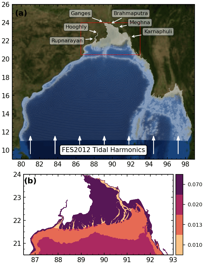
Figure 2(a) Model domain with arrows indicating the open boundaries. (b) Distribution of Manning coefficient. The background used in (a) is taken from Blue Marble: Next Generation, credited to NASA Earth Observatory.
Hydrodynamically, our model is bounded on the ocean and the riverfronts, with the no-slip condition for momentum along the closed boundaries. Along the ocean boundary, we have implemented a tidal water level derived from the 26 dominant tidal constituents of the global FES2012 tidal atlas (Carrère et al., 2013). Sensitivity tests between FES2012 and FES2014 (Lyard et al., 2021) did not yield any significant difference for our model domain. The applied constituents are M2, M3, M4, M6, M8, Mf, Mm, MN4, MS4, Msf, Mu2, N2, Nu2, O1, P1, Q1, R2, S1, S2, S4, Ssa, T2, K2, K1, J1, and 2N2. In total, we implemented six open riverine boundaries. For the rivers Ganges, Brahmaputra, Meghna, Hooghly, and Karnaphuli, we have prescribed a discharge boundary condition. We have implemented a radiating boundary condition for the Rupnarayan river. To mimic the observed seasonal pattern of sea level reported by Tazkia et al. (2017), we have implemented a harmonically varying sea level along the southern boundary with a period of 1 year and an amplitude of 35 cm, peaking in August. Over the whole domain of the model, the astronomical tidal potential is also forced for 12 constituents (2N2, K1, K2, M2, Mu2, N2, Nu2, O1, P1, Q1, S2, T2).
The bottom friction is parameterized using Manning’s n. We adopted an approach for the spatial distribution of the Manning coefficient similar to Krien et al. (2016) and the one used in Khan et al. (2021a) (Fig. 2b). For the deeper part of the ocean (depth > 20 m), we used a Manning coefficient value of 0.02. In the nearshore zone, the Manning coefficient was set to 0.013. In the rivers, a Manning coefficient value of 0.01 was set. Unlike in Krien et al. (2016), for the inland area, we adopted a Manning coefficient value of 0.07, which is more reasonable for a vegetated land like the Bengal delta (Bunya et al., 2010).
2.2 Coupling with wave model
Our modelling framework is coupled online with the spectral Wind Wave Model III (WWMIII) at the source code level (Roland et al., 2012). WWMIII solves the wave action equation over the same unstructured grid as the hydrodynamic core. It considers source terms for the energy input from wind (Ardhuin et al., 2010), non-linear interaction in deep and shallow water and energy dissipation due to white-capping, wave breaking, and bottom friction. We modelled the wave breaking using the formulation of Battjes and Janssen (1978). A low value of the coefficient of breaking, α=0.1 (instead of α=1), is adopted to avoid over-dissipation over a very mild slope region like the Bengal delta (Pezerat et al., 2020, 2021; Khan et al., 2021a). We have discretized our modelled spectra into 12 directional and 12 frequency bins. For the current resolution of the model (e.g. 250 m at the nearshore), we found that the sensitivity of the resulting wave set-up is negligible compared to higher-resolution discretization of the spectra (36 directional and 24 frequency bins). The coupled model is solved with implicit schemes, which allows large coupling time steps. In our model configuration, SCHISM and WWMIII were set up to exchange water level and current every 30 min.
2.3 Wind and pressure fields
During a cyclone, the momentum transfer from the wind to the water column and the inverse barometer effect of the pressure drop are the primary driver of the storm surge. Thus, an accurate enough representation of the wind and pressure fields in a numerical modelling framework is of prime importance. In some well-monitored basins, there are extensive networks of observational data which can provide relatively accurate wind and pressure fields during a storm. However, the observations of these variables over the Bay of Bengal are virtually non-existent. As such, the wind and pressure fields during a cyclonic storm have to be estimated from either numerical weather models or satellite observations. Due to the high error associated with the commonly available numerical weather models, it is a fairly common practice in storm surge modelling to infer the wind and pressure fields from parametric cyclone models (Lin and Chavas, 2012). As the computation of parametric wind and pressure fields is comparatively light, this approach is also useful for sensitivity studies based on various configurations of a single storm (e.g. Hussain et al., 2017) or from a large ensemble of synthetic cyclones (e.g. Krien et al., 2017a).
The associated error with these parametric cyclone models varies with distance from the centre of the storms (Krien et al., 2018). The most considerable uncertainties in estimating wind and storm are from the surface wind reduction factor (SWRF) and the choice of gradient wind profile (Lin and Chavas, 2012). From a comprehensive comparison of parametric cyclonic wind fields with scatterometer observations for 16 storms, Krien et al. (2018) showed that the relative error in the wind field is minimized with a combination of parametric wind fields. Following their findings, we have used a combination of Emanuel and Rotunno (2011) and Holland (1980) formulations to derive the parametric wind profile. We have applied a SWRF of 0.9 (Lin and Chavas, 2012; Krien et al., 2017b). The effect of storm translational speed is accounted for through a surface background wind reduction factor of 0.56 and a counter-clockwise rotation angle of 19.2∘ as suggested by Lin and Chavas (2012). In all cases, we used the Holland (1980) model to derive the pressure field. See the Supplement for further details.
2.4 Validation
The performance of our model in simulating the tide was documented in previous studies (Khan et al., 2019, 2020). We found that our model has a 2 to 4 times better reproduction of tidal water level compared to global tidal models and comparable performance with the previous state-of-the-art models in this region (Krien et al., 2016). The total complex error calculated over four major tidal constituents – M2, S2, K1, and O1 – ranges from 5 to 20 cm, which is comparable to other well-documented shorelines around the world. Notably, the current model shows better performance around the mouth of Meghna estuary – a critical region with complex hydro-morphodynamics (see the Supplement).
The observational network of tide gauges is sparsely distributed and typically non-functional during an intense cyclone (Krien et al., 2017b). It is thus relatively difficult to achieve a thorough assessment of the model realism for most of the historic cyclones. The quality of the tide gives a preliminary assessment of the potential skills of our model in simulating storm surges. Given that the wind and pressure fields are adequately prescribed and that necessary physics – particularly the wave coupling – are incorporated, the model is expected to simulate a storm surge appropriately.
In Khan et al. (2021a), the performance of the model used in this study in simulating storm surges is demonstrated through a hindcast of the surge generated by a recent cyclone – Amphan – that made landfall in this region. From a set of in situ observations, it was found that the model performs well (5–10 cm peak water level error) in reproducing the maximum water level observed at multiple tide-gauge locations distributed throughout the Bengal shoreline.
To supplement the results shown in Khan et al. (2021a), we also performed a hindcast of the water level generated by cyclone Sidr – another comparatively well-documented historic cyclone (Krien et al., 2017b). Figure 3 shows the water level evolution at four tide gauge stations around the landfall location. The modelled water level is shown as black lines, and the observed water level records are shown as dots. As noted by Krien et al. (2017b), the tide gauge stopped working at Khepupara at the time of very high water. The error of the peak modelled water level typically amounts to 10–20 cm. It should be noted that, in their hindcast, Krien et al. (2017b) shifted the time of landfall by half an hour to get a better match of the timing of the peak water level. Here we retained the original Joint Typhoon Warning Center (JTWC) track, hence the slight shift in phase of the water level. Moreover, both Krien et al. (2017b) and Khan et al. (2021a) combined their analytical wind and pressure fields (around the storm centre) with a background field (far from the storm centre) taken from global atmospheric models. Here we used only the analytical wind fields to be consistent with the forcing strategy used for the storm surge computation from the cyclone ensemble (Sect. 3). The results from this experiment illustrated in Fig. 3 show that the peak water levels around the landfall are captured well. This peak water level is the main variable we will deal with in our storm surge hazard assessment.
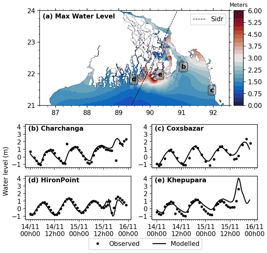
Figure 3(a) Maximum simulated water level during cyclone Sidr. Comparison of simulated and observed water level during cyclone Sidr at (b) Charchanga, (c) Cox's Bazar, (d) Hiron Point, and (e) Khepupara. The station locations are shown in (a).
In summary, the results of these experiments – cyclone Amphan (Khan et al., 2021a) and cyclone Sidr (this section) – show that our model can successfully reproduce water level evolution, as well as maximum water level, during cyclones along the shoreline of the northern Bay of Bengal.
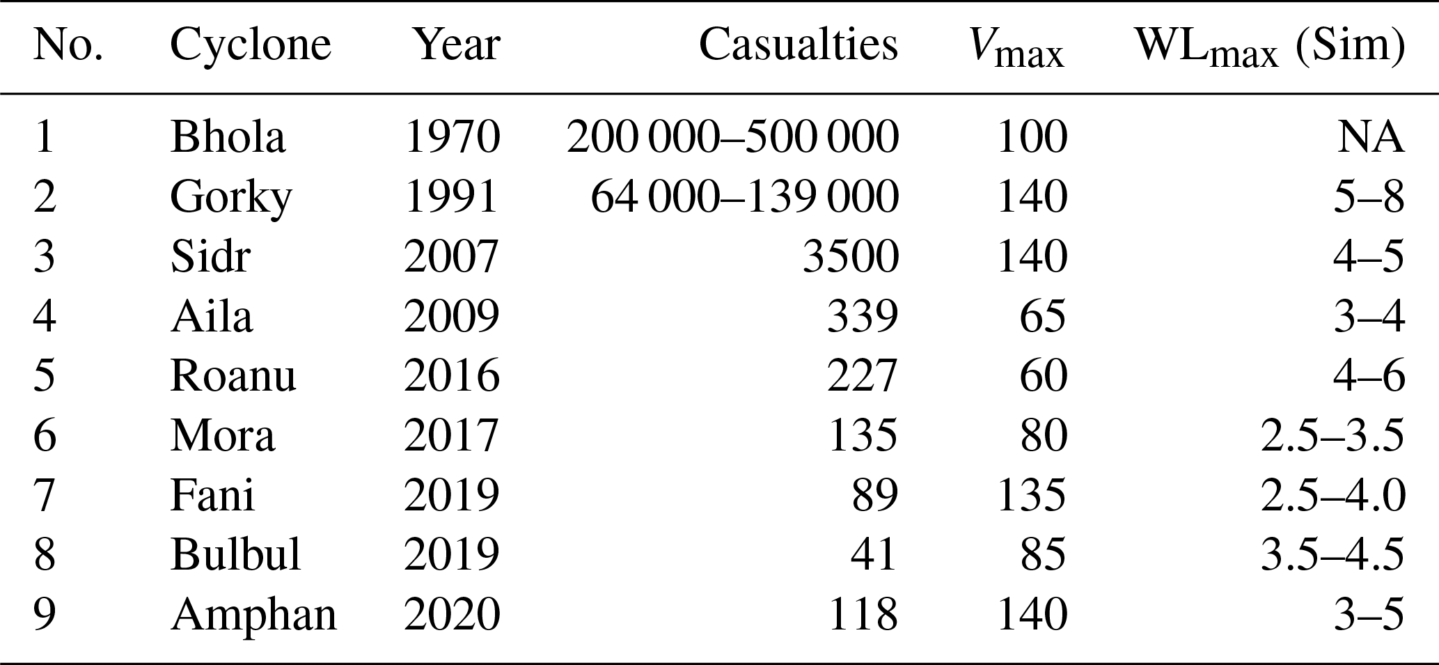
In addition to the validation experiment described above, we performed a hindcast for the cyclones shown in Fig. 1. The corresponding maximum water level estimates from our model are listed in Table 1. We adopted the JTWC best track dataset for the cyclones' track and intensity information. For the 1970 Bhola cyclone, the intensity of the cyclone was not available in the JTWC dataset. The motivation for doing so is not validation. As illustrated by Krien et al. (2017b) validating for past cyclones is often difficult due to the limited availability of water level data, which is further aggravated by the failure of the tide gauge during cyclonic storms. The objective is rather to illustrate the typical variation in maximum water level that can occur during a cyclone along the Bengal delta shoreline.
Table 1Simulated maximum water level for the cyclones shown in Fig. 1. Vmax is the maximum wind speed in knots, and WLmax (Sim) is the simulated maximum water level range over the delta shoreline in metres. NA signifies not available.
3.1 Synthetic storm dataset
Here we use a large ensemble of 3600 synthetic storms passing by the lower part of the Bengal delta. These synthetic storms were generated through the statistical–deterministic approach of Emanuel et al. (2006) based on the climatic conditions of the 1981–2015 period. The forcing background climate is derived from the National Center for Environmental Prediction/National Center for Atmospheric Research (NCEP/NCAR) reanalysis (Kalnay et al., 1996). In this method, synthetic storms are generated in three steps. First, a synthetic environmental wind field is derived from a long-term dataset which conforms to the mean climatology. For our ensemble of storms, the environmental wind field is derived from the NCEP/NCAR reanalysis dataset for the zonal and meridional wind components at 250 and 850 hPa. During this step, the observed monthly means and variances are respected, as well as most of the covariances. Monthly means of sea surface temperature and atmospheric temperature and humidity are also used. In the second step, a set of tracks is generated from a random field of genesis points and a weighted mean of 250 and 850 hPa wind plus a correction for beta drift (Emanuel et al., 2006). The weight factor is tuned to best match observations of track displacements, and the rate of seeding is calibrated to match overall observed storm frequencies. Finally, the storm intensity is estimated along the tracks using a coupled ocean–atmosphere one-dimensional axisymmetric model with parameterized effects of vertical wind shear (Emanuel et al., 2004). The wind shear is given by the synthetic time series of winds determined previously. The output of this axisymmetric model is essentially the parameters of the radial structure of the pressure and wind field, expressed as along-track series of central pressure, maximum wind speed, and the radial distance from the centre of the storm where this maximum wind speed prevails. Previous applications of this model include the assessment of storm surge hazard in Guadeloupe (Krien et al., 2015) and Martinique (Krien et al., 2017a), storm surge return period in New York City (Lin et al., 2010), and the estimation of wind return period in Boston and Miami (Emanuel et al., 2006).
Given that our geographic interest is focused on the Bengal delta, the cyclone ensemble comprises only the cyclones that pass through a 300 km radius centred on the centre of the delta (defined at 21.71∘ N, 89.57∘ E). The cyclone generation model was adjusted using a calibration factor based on the observed cyclone genesis and displacement characteristics in the JTWC dataset. The calibration factor was set to 1.2, which indicates the rate of seeding for cyclone genesis in the probabilistic cyclone generation model. With an average annual frequency of 0.7 cyclones, the ensemble of 3600 cyclones considered here represents more than 5000 years of cyclonic activity over the northern Bay of Bengal under present climate conditions. The frequency of cyclones making landfall along the shoreline (for each 20 km × 20 km pixel) is shown in Fig. 4a. The inset of Fig. 4a shows a subset of the cyclone tracks in the ensemble.
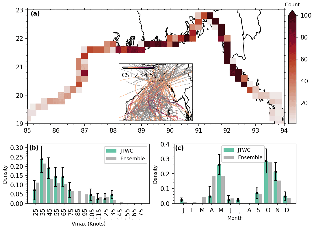
Figure 4(a) Spatial distribution of the paths of the cyclones that make landfall along the coast of Bengal delta. Each square bin is 20 km wide. A small subset of cyclone trajectories is shown in the inset. (b) Distribution of maximum wind speed of the synthetic cyclones compared to the JTWC dataset. (c) Annual distribution of the occurrence of the synthetic cyclones compared to JTWC dataset. In (b) and (c), the error bar indicates the standard error associated with the small sample size in JTWC dataset.
This synthetic ensemble of storms is fundamentally different from the hypothetical storms employed in past studies, e.g. Hussain et al. (2017). Hypothetical storms are typically generated from a known storm by modifying its track or strength or both, which could render some storms unrealistic. On the other hand, the storms in our ensemble are physically meaningful and statistically consistent. The consistency of the cyclone ensemble is illustrated through a comparison with the observed JTWC statistics for maximum wind speed (Vmax) (Fig. 4b) and seasonal distribution (Fig. 4c). Error bars in both cases indicate the standard error of the observation (i.e. short length of dataset) given the probability distribution in the ensemble computed assuming a Poisson process. A similar standard error estimate is obtained using a bootstrap method (see the Supplement).
The distribution of the simulated maximum wind speed (Vmax) shows a good agreement with the observations from JTWC (Fig. 4b). The standard errors for the JTWC dataset indicate that the ensemble distribution of (Vmax) is within the range of observational uncertainty.
Similarly, the seasonal distribution of the cyclone ensemble and that observed from JTWC both show a well-matching pattern with a bimodal seasonality (Fig. 4c) (Alam and Dominey-Howes, 2014). In the Bay of Bengal, low-pressure systems typically cannot intensify into a storm due to strong vertical wind shear present during monsoon (June–August). During the pre-monsoon (March–May) and post-monsoon (September–November), low vertical wind shear and high sea surface temperature provide a suitable condition for low-pressure systems to intensify. For all months, except April, the ensemble cyclone density is typically within the range of observational uncertainty indicated by the error bar (Fig. 4c). However, for our storm surge hazard analysis, no measurable impact is expected from such intra-seasonal differences in cyclone distribution. The overall simulated bimodal temporal evolution of the synthetic cyclone indicates that the temporal statistics captured by our statistical–deterministic method correspond well with the seasonal climatic characteristics.
3.2 Storm-surge-induced water level estimate from the ensemble
Estimation of the extreme water levels associated with the storms in the ensemble is done in two steps. First, for each synthetic storm, the wind and pressure fields are derived, as explained in Sect. 2.3. For the wind fields, we again employed a combination of parametric models based on the findings of Krien et al. (2018) to minimize the bias in individual parametric models. Here, for the inner core of the cyclones (r<r50), the wind field is estimated using the model of Emanuel and Rotunno (2011). On the outer core (r>=r50), we used the Holland (1980) model. The pressure field is estimated from the formulation of Holland (1980) for all radial distances. The wind and pressure fields are updated every 15 min with a linear interpolation of the associated variables.
Second, with wind and pressure fields, we calculate the ensemble of water level estimates using the same ocean–wave coupled model set-up used for the hindcasts described in the previous section. We achieved this ensemble of water level estimates through individual simulations of each of the 3600 storms – which amounts to 14 years worth of model simulations. Along the open boundaries of the rivers Ganges, Brahmaputra, and Meghna, we have prescribed a time series of observed discharge sampled at the timestamps of the cyclones, which ranges from 1980 to 2015. We have applied a discharge climatology as the boundary condition for Hooghly (Mukhopadhyay et al., 2006) and Karnaphuli (Chowdhury and Al Rahim, 2012). Applied tidal forcing and the tidal water level boundary are also consistent with the timestamps of the synthetic cyclones. Similar to the model set-up used for the hindcast experiments, we have also taken into account the seasonal mean sea level variation in the Bay of Bengal by applying an annual harmonic on the water level along the oceanic open boundary with a period of 1 year peaking in August with an amplitude of 35 cm, as in Tazkia et al. (2017). The coupling between SCHISM and WWMIII allows for accounting for the wave set-up induced by the radiation stress gradient of the waves (Longuet-Higgins and Stewart, 1964). Similar to the model set-up for cyclone Amphan hindcast in Khan et al. (2021a) and for the Sidr hindcast in this paper, the breaking coefficient (α) is set to 0.1 (instead of the default parameter α=1) to avoid over-dissipation of the waves over the submarine part of the delta with mild slopes (Pezerat et al., 2021; Khan et al., 2021a). We also invoked the wetting and drying algorithm in SCHISM with a threshold of 10 cm depth of water for an element to be registered as wet.
3.3 Statistical analysis methodology
We have applied ranking-based statistical analysis to infer the quantities at a given return period. To do so, at each node the quantity of interest (e.g. maximum water level, maximum surge level) is first sorted sequentially among the 3600 members, from the smallest value to the largest one. As we mentioned, since our dataset consists of 3600 cyclones with a yearly frequency of 0.7 cyclones, it corresponds to 5120 years of cyclonic activity. Once sorted in ascending order at each point of the model grid, each water level present in the sorted ensemble corresponds to a return period ranging from 5120 3600 viz. 1.42 years (for the smallest return period) to 5120 years (for the largest return period). We have used a bootstrap technique to compute the confidence interval for the return level estimates (Hesterberg, 2011). Unless otherwise stated, we have pooled 10 000 bootstrap samples of the same size as our ensemble (3600 cyclones) with replacements and applied the above-mentioned ranking method without considering ties.
Estimated quantities at return periods between 5 years and 500 years (at 5-year steps) are considered trustworthy in our subsequent analysis to make sure that our ensemble contains a large enough sample for each return level. Over the whole Bengal delta at the 500-year level, the number of individual unique cyclones that contribute amounts to about 50 (viz. an average of three cyclones per 20 km of shoreline). Above 500 years, the sample size for cyclones that contribute to the return period is smaller, which is potentially too small to capture the extreme value statistics. The robustness of our results for the selected return periods will be discussed further in Sect. 4. We linearly interpolated the water level at individual integer return periods (in years) from the ranked dataset.
The outcome of the statistical analysis consists of water level maps at various return periods, spatially distributed on our model grid. Figure 5a shows the water level at the 50-year return period over the northern Bay of Bengal. The meaning of the colour bar is twofold. At all grid points located below mean sea level, including the estuaries, the colour indicates the water level above the mean sea level. At the grid points located above mean sea level (e.g. inland), the colour indicates the inundation depth above topography. This water level at the 50-year return period is computed from the full ensemble of cyclone simulations using the empirical statistical method described in Sect. 3.3, pixel-by-pixel. As such, the total water level at the 50-year return period has contributions from hundreds of different cyclones of our ensemble. In our estimate, about 600 individual cyclones contribute to the 50-year return period water level over the illustrated region. To supplement subsequent discussions, in Fig. 6 we also present the water level estimates and corresponding 95 % confidence intervals at a few station locations for a range of return periods (up to 500 years). These station locations are shown as black stars in Fig. 5.

Figure 5(a) Inundation extent and corresponding water level at a 50-year return period. Black stars indicate the station locations for the results shown in Fig. 6. (b) Mean high water (MHW) derived from a year-long tidal simulation. (c) Water level for the 50–500-year return periods expressed as a multiple of the MHW level along the nearshore dash-dotted line shown in (a) and (b).

Figure 6Extreme water level evolution with return period at (a) Sagar Roads, (b) Hiron Point, (c) Charchanga, (d) Chittagong, (e) Diamond Harbour, and (f) Chandpur. These station locations are shown in Fig. 5. The shaded grey area indicates the 95 % confidence interval.
The 50-year return period water level shows a similar spatial pattern as the mean high water, as shown in Fig. 5b, as well as the tidal range (Khan et al., 2020). We see that a dipolar pattern arises, with a very high water level in the north-eastern (around 88∘ E) and the north-western (around 91.5∘ E) corners of the bay. In contrast, in the central region (between 88.5 and 91∘ E), there is a local minimum of about 2.25–2.5 m in the estimated 50-year return period water level. However, among these two maxima, the 50-year water level in the north-eastern part reaches about 6m, twice as much as the 50-year water level in the north-western part of the delta (barely 3 m). At a 50-year return level, these estimates of water levels are objectively robust along the open coastlines, as well as inside the estuaries, with a couple of centimetres range in the computed 95 % confidence interval (Fig. 6).
Inland, at a 50-year return period, a contrasting flooding pattern is observed. Two specific regions are found to be flooded by a storm surge at a 50-year return period – one around 21.5–22.5∘ N, 89–90∘ E and another around 22.5–23.5∘ N, 90–91∘ E. The first inundated region is the Sundarbans mangrove forest, which spans across the border between Bangladesh and India. The region is a sanctuary and legally protected region and thus devoid of any engineering intervention, like embankments. The second inundated region along the Ganges–Brahmaputra–Meghna (GBM) estuary, in contrast, is densely populated. According to the polder embankment dataset used in our modelling, this region is not protected by the coastal polder network and is thus exposed to the risk of flooding. Other than these two regions, the sea-facing inland areas are primarily found to be not flooded at a 50-year return level. These regions are protected by polder embankments (typically earthen) (Khan et al., 2021a), hence creating this contrast in the pattern of the flooded area.
Along the delta coastline facing the open ocean, the 50-year return period water level appears to be in contrast, as we saw. To further illustrate this, we extracted the water level at the various return periods along the black line shown in Fig. 5a–b, and we display it in terms of multiples of the mean high water level (MHW) along the line (Fig. 5c). The MHW level, shown in Fig. 5b, is calculated from a 1-year-long tidal simulation and taking the mean of daily (25 h) tidal high-water estimates. Our motivation for such a display stems from the similarly contrasting range of MHW along the shoreline – with two macrotidal poles in the north-western and north-eastern corners reaching around 2 m (at 88∘ E) to 3 m (at 91.6∘ E) and a dip of 1 to 1.25 m around 90∘ E to 91∘ E. From Fig. 5c, it can be seen that throughout the cross-section, the 50-year return period water level is around twice as much as MHW or higher. The increase in water level with the return periods along this nearshore cross-section shows regional sensitivity. From the mouth of Hooghly estuary to the region of the Sundarbans mangrove forest (88∘ E–89.5∘ E) the water level evolves moderately, with the return period showing only a 50 % increase from the 50-year return period to 500-year return period. On the other hand, when approaching the mouths of the Meghna estuary, between 90.5∘ E and 91∘ E, the pluri-centennial water level increases sharply with the return period to reach more than twice the 50-year return period water level for the 500-year return period. The maps of water level over the delta obtained for return periods ranging from 5 to 500 years are shown in Fig. 7. The regional pattern of water level at various return periods consistently shows the same bi-polar pattern throughout the return periods investigated here, from the 5- to 500-year return periods (Fig. 7). Throughout these return periods, the confidence interval of the estimated water levels along the open coastline remains reasonably tight (Fig. 6a–d). At lower return levels (5 to 200 year), the confidence interval range remains typically below 5 % of the water level estimate. At higher return levels (200 to 500 year), the confidence interval range is comparatively tighter for the central part of the delta, reaching about 10 % of the water level (Fig. 6b). On the eastern (Fig. 6c–d) and western poles (Fig. 6a), the confidence interval range varies between 15 % and 20 % of the water level estimate.
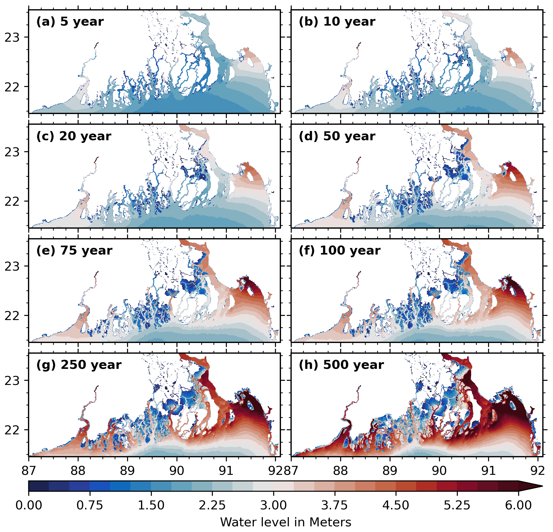
Figure 7Inundation extent and corresponding water level at (a) 5-year, (b) 10-year, (c) 20-year, (d) 50-year, (e) 75-year, (f) 100-year, (g) 250-year, and (h) 500-year return periods.
The inundations in the mangrove region around 89.5∘ E seem to have a large saturation effect on the evolution of the return period of the water level. There the water level remains practically the same for the various return periods, slightly rising from 2.5 m at a 50-year return period to 3 m at a 500-year return period with a tight confidence interval (Fig. 6b). We also see this evolution in Fig. 7.
The flooding extent in the estuaries and adjoining areas changes significantly from the short return periods to the longest ones (Fig. 7). We selected the three main estuaries to take a closer look at the evolution of water level with the return periods. These are GBM on the eastern side (Fig. 8a–b), Pussur estuary in the central mangrove region (Fig. 8c–d), and Hooghly estuary on the western side (Fig. 8e–f). The water level at the various return periods is extracted along the lines shown in Fig. 8a, c, and e and shown as a multiple of the 50-year return period water level in Fig. 8b, d, and f.
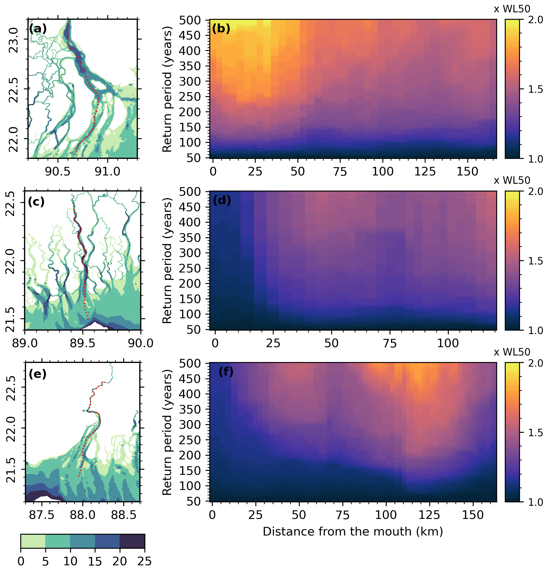
Figure 8Water level as a function of the return period, expressed in multiples of the 50-year return period water level along the dashed lines shown in red for (a–b) Ganges–Brahmaputra–Meghna estuary, (c–d) Pussur estuary, and (e–f) Hooghly estuary. The x axis is the distance from the mouth of the estuary in kilometres. The background shading in panels (a), (c), and (e) shows the bathymetry in metres.
In the GBM estuary, the water level increases sharply with increasing return period along the whole cross-section considered here, as shown in Fig. 8a–b. Over the downstream-most 50 km, the 500-year return level reaches more than twice the 50-year return level. Further upstream, up to the estuarine bottleneck of Chandpur (23.24∘ N), the sensitivity of the water level to the return period is more moderate, with around 50 % higher water level at a 500-year return period compared to the 50-year return level. At 95 % confidence interval these patterns remain robust from the mouth (Charchanga, Fig. 6c) to Chandpur (Fig. 6f).
In the Hooghly and Pussur estuaries, a contrasting pattern is observed compared to GBM – the water level for the longer return periods rises much more sharply in the upstream part than in the downstream part. Along the Hooghly estuary, the sensitivity of the water level to the return period is moderate for the first 100 km but amplifies considerably further upstream. This amplification appears to be linked to the changes in the tide along the estuary (see the Supplement). The 95 % confidence interval of the water level estimate inside the Hooghly estuary (Diamond Harbour, Fig. 6) is also considerably wider after the 250-year return period.
Along the Pussur estuary, weak variation in the water level across the various return periods is seen over the first 25km and then shows a moderate evolution towards upstream. These upstream patterns remain robust at 95 % confidence interval, as shown for Hiron Point (Fig. 6b) which is located 30 km from the mouth.
5.1 Synthetic cyclone ensembles statistics
The synthetic cyclone dataset used in this study makes our estimation inherently different from most of the previous attempts to map the storm surge hazard along the shoreline of the Bengal delta. The underlying statistical–deterministic approach of our storm database provides three significant improvements over the previous approaches used over the Bengal delta. First, the random genesis of the storms induces a probabilistic nature of the population of the storms. Second, the deterministic evolution of the storms makes sure that the resulting population of tracks are physically valid, which is consistent with the ocean–atmosphere coupling to a reasonable extent. The resulting statistical distribution of maximum wind speed of the storms shown in Fig. 4b gives confidence in the capability of the statistical–deterministic approach to capture the actual behaviour of the ocean–atmosphere system over the Bay of Bengal. Third, a large enough population of storms allows both an appropriate spatial coverage of the coastline and appropriate temporal coverage of the pluri-annual to pluri-centennial return periods of interest here (Fig. 4a, c).
The distribution of the cyclones along the shoreline shown in Fig. 4a illustrates a dense population of cyclones making landfall along the convex delta front (88∘ E–91∘ E). A large number of storms is also observed along the eastern coast of Bangladesh. This landfall pattern corresponds to previous observations that the cyclones making landfall on the Bangladesh coastline tend to move north-eastward (Ali, 1996; Akter and Tsuboki, 2021; Mondal et al., 2021).
5.2 Inundation extent and consistency
The storm surge inundation hazard has significant spatial variability across the Bengal delta region (Fig. 5). Our underlying statistical analysis is an empirical rank-based return period estimation, which requires the ensemble size to be large enough to achieve a smooth spatial and temporal resolution. Visibly, the water level estimation at the 50-year return period shown in Fig. 5a follows a smooth pattern over the Bengal delta region. In our estimate, about 600 and 400 unique cyclones contribute to the 50- and 100-year return period water levels, respectively. In other words, for a given return period the associated water level is pulled in from a large number of individual cyclones, which in turn includes cyclones with a range of intensities making landfall at various phases of the tide. Indeed, this spatial smoothness of water level is observed for all the return periods we analysed from 5 to 500 years (Fig. 7), indicating a robust estimate of the storm surge water level. The confidence interval for the water level estimate for the 5- to 500-year range of return periods presented in Fig. 6 corroborates the robustness of our estimate.
It appears that the water level has a similar regional distribution as tidal amplitude with two maxima in the north-eastern and north-western corners and a relative minimum in between (Fig. 5a–b). At the mouth of Hooghly, in the north-western corner of the delta, the 50-year return period water level is about 3.5 m. The 50-year water level reduces to about 2 m when moving eastward at the mouth of the Pussur river. Further eastward the water level increases again to reach about 6 m along the shoreline of Sandwip Island (22.5∘ N, 91.6∘ E) and Chittagong (22.5∘ N, 91.7∘ E). This estimated water level is on average twice as much as the mean high water level (Fig. 5c). We found the highest 50-year return period water level at the eastern side of the mouth of Meghna estuary (90∘ E–91∘ E). There the 50-year return period water level reaches thrice as much as the mean high water.
5.3 Comparison with previous estimates
As mentioned previously, a reliable estimate of the return period of storm surge water level over the Bengal delta has not emerged due to the gap in data, as well as modelling limitations. A comparison is presented here with the previous estimates by Lee (2013) and Jakobsen et al. (2006). Lee (2013) did an extreme value analysis of the observed time series over 1977–2009 (33 years) at Hiron Point tide gauge located on the central Bengal shoreline (21.8∘ N, 89.5∘ E). For this purpose, he decomposed the time series using the ensemble empirical mode decomposition approach. He reconstructed the water level by only keeping the very high-frequency (∼ 3 h) and very low-frequency modes. This process essentially removed the tide from the water level and retained the de-tided residual (i.e. surge). Using a yearly maximum method, in his extreme value analysis, he obtained a 1.66 m [1.50–1.95] surge level at a 50-year return period and 1.75 m [1.57–2.14] at a 100-year return period. The range in the parentheses is the 90 % confidence interval.
In the previous section, our analysis was focused on the water level rather than surge level. To compare with the estimate of Lee (2013), we reprocessed the whole ensemble of storm event simulation results. We have first extracted the tidal water level from the 3600 cyclones that we simulated. Then, for each cyclone, we extracted the maximum surge level. Finally, on this maximum surge estimate, we applied the same ranking-based return period estimate. At Hiron Point, our estimation of surge amounts to 1.77 m [1.68–1.85] at 50-year and 2.31 m [2.12–2.47] at 100-year return periods. The range in the parentheses is the 90 % confidence interval. At a 50-year return period, with a difference of only 14 cm (inferior in Lee, 2013), our estimated value is comparable to the estimated value by Lee (2013) from the observation time series. The confidence interval was twice narrower compared to Lee (2013). It should be noted that the estimated 50-year return period water level from our ensemble is about 3 m at Hiron point. At a 100-year return period, the estimate of Lee (2013) was underestimated compared to ours by 56 cm.
The evolution pattern of 50-year return period water level is consistent with the previous estimates but with varying degree of agreement on the amplitude (Jakobsen et al., 2006; Sindhu and Unnikrishnan, 2011). From an ensemble of 17 historic cyclones, Jakobsen et al. (2006) estimate that the 100-year return period water level reaches about 5 m at the mouth of Meghna and about 8–10 m around Sandwip (see their Fig. 5). A similar pattern has emerged in our analysis but with a much different water level estimate. We estimate that the 100-year return period water level is about 4 m at the mouth of Meghna, reaching about 6 m around Sandwip. In general, the water level estimates of Jakobsen et al. (2006) are consistently larger than the ones presented here. It is noteworthy that the modelling framework of Jakobsen et al. (2006) does not take into account the wave set-up. However, the limited and potentially biased sampling of the “strongest” cyclones (17 in total, over 40 years) leads to an overestimation of the storm surge level.
Along the eastern part of the West Bengal shoreline (87∘ E–88∘ E), Sindhu and Unnikrishnan (2011) found an increase in water level when moving northward. Similar to Jakobsen et al. (2006), the pattern of water level they estimated is similar to ours, but their values are significantly larger than ours. At Sagar Island, their estimated 5- and 50-year return period water levels are 6.92 and 8.74 m, respectively. In our estimation, the 5- and 50-year return period water levels are 2.75 and 3.5 m above mean sea level, respectively. It is not clear if the estimate of water level provided by Sindhu and Unnikrishnan (2011) is relative to mean sea level. It should be noted that the mean estimated high water at Sagar Island is about 1.75 m above mean sea level, which is only one-fourth of the estimated 5-year return period water level (6.92 m) by Sindhu and Unnikrishnan (2011).
Leijnse et al. (2022) used a somewhat similar approach to ours. They used an extreme value analysis on the surge estimate of 1000 year simulated cyclonic activity using peak-over-threshold (POT) method and an exponential fit. In their estimate, the surge level (from tide-free simulations) at Charchanga and Chittagong at a 100-year return period is about 2.8 m [2.5–3.1] and 3.3 m [3.1–3.6], respectively. The range in the parentheses is the 95 % confidence interval. To compare with the estimate of Leijnse et al. (2022) we have re-simulated the ensemble of our 5000-year cyclonic activity (3600 cyclones) again but without incorporating the tide. In our estimate, the 100-year return period surge level is 3.6 m [3.4–4.0] and 4.1 m [3.8–4.3] for Charchanga and Chittagong, respectively. In other words, in these two locations, the estimate of Leijnse et al. (2022) is more than 60 cm lower than ours, while the confidence interval range between their study and ours is essentially the same.
Several factors might underlie this difference between the estimate by Leijnse et al. (2022) and ours. As discussed before, the modelling framework of Leijnse et al. (2022) is an extraction of a global model relying on global bathymetric data which suffers from large bias in the northern Bay of Bengal region (Krien et al., 2016). The model resolution used in Leijnse et al. (2022) is also kilometric (3 km or higher for the unstructured-grid hydrodynamic model, 2 km for the structured-grid wave model), which is not enough to model the complex shoreline and shallow coastal domain of the northern Bay of Bengal, particularly the wave breaking and associated set-up. The parameterization of the wave breaking model might also not be well tuned for the very mild slope of this region (inferior to ). As shown by Pezerat et al. (2021), the default parameterization in wave breaking models can induce over-dissipation over such mild slope regions and underestimate the wave set-up by as much as 100 %. Additionally, no discharge is imposed along the Ganges–Brahmaputra where the surge can interact with the river discharge and propagate far inland (Khan et al., 2021a). Finally, Leijnse et al. (2022) used extreme value analysis based on the POT method and exponential distribution fitting to infer the return period surge level, which could induce further error linked with the choice and fitting of the distribution, as well as the threshold for the POT method.
5.4 Return period of previous cyclones
From the hindcasts of previous cyclones – cyclone Sidr and cyclone Amphan – a wide regional variation in the return period of the maximum water level during storm surge is found.
The maximum water level estimates from our hindcast of the Sidr cyclone (see Fig. 3) shows a strong surge near the landfall location where it reaches 6 m along the shoreline of Kuakata and remains strong in the connected tributaries. This water level amounts to a return period of about 500 years. At the same time, the maximum water level hindcast along the coast of Chittagong and Sandwip is about 4.5 m, which corresponds to a roughly 50-year return period water level at that location (Fig. 7).
Compared to Sidr, the regional variation in maximum water level is much less pronounced for cyclone Amphan (Khan et al., 2021a, see their Fig. 5). The maximum modelled water level reached about 5 m around 88.4∘ E, which corresponds to a 250-year return period (Fig. 7). At the landfall location of Sidr (around Kuakata), about 100 km eastward, the maximum water level is estimated to be 2.5 m, corresponding to a 50-year return level. Similar to Sidr, the water level along the Sandwip coast during Amphan reached about 4.5 m, i.e. a 50-year return level.
5.5 Role of embankments
From the various maps of n-year return period inundation extent and water level shown in Fig. 7, it is clear that the embankments play a vital role in the storm surge flooding. Although these embankments were established for controlling tidal intrusion to promote agricultural activity, the initial designed heights appear to be relevant, providing considerable protection during extreme events. Our estimate shows that, under current climate cyclonic activity, for the embankment heights implemented in our model, the embankments start overflowing at the 75- to 100-year return period water levels (Fig. 7).
The level of embankment protection estimated here must be taken with caution as we are limited by the availability of the embankment information and up-to-date status report. These earthen embankments are poorly maintained (Islam et al., 2011), whereas our modelling approach essentially assumes that their geometry is constant in time (implying that they can not be altered by any devastating cyclone typically). This is not the case as shown by Khan et al. (2021a) in their newspaper survey, in which they found the breaching of the embankment to be the prevalent cause of flooding inside a polder during cyclone Amphan. The information of embankments’ height used in the model of this study is more than a decade old. The actual current height of these embankments is unknown. Additionally, in our embankment height dataset, only one value of height is provided across each of the embankments. In reality, we expect a spatial variation in embankment height. Considering all these factors, the estimated level of return period when the embankments start overflowing might be overestimated. In other words, the embankments are estimated to be overflowed at a higher return period water level event, when in reality it is overflowing at a lower return period.
5.6 Population exposure
Storm surge is a significant hazard for the large population that lives in the Bengal delta. Figure 9 shows the population density in Bangladesh part of the delta area with a grey colour bar based on the Global Human Settlement (GHS) population dataset of 2015 (Schiavina et al., 2019). This dataset is based on the GPWv4 dataset (CIESIN, 2016) illustrated in Fig. 1 but disaggregated from the original administrative- and/or census-level data to a grid-cell-based distribution of the built-up areas (Freire et al., 2016). The contours of the flooding extent at return periods ranging from 5 to 500 years are shown in colour.
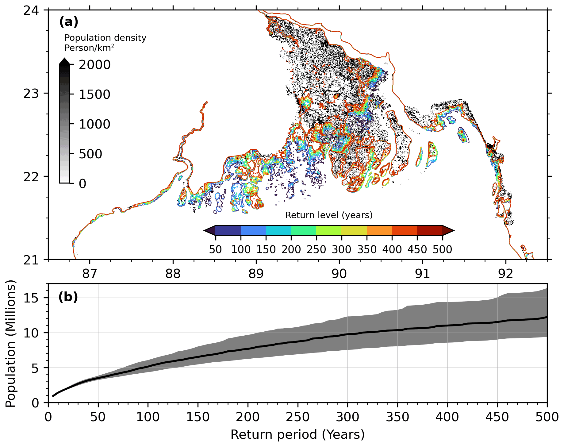
Figure 9(a) Spatial coverage of flooding at various n-year return periods estimated from the model. The grey colour bar shows the population density per square kilometre. (b) Number of people affected at various n-year water level return periods. The shaded area shows the 95 % confidence interval.
As the population data are provided on a regular latitude–longitude grid and the model grid is unstructured, it is first necessary to map the inundation over the population dataset. We took the following steps for mapping.
-
We interpolated the modelled return period water levels to the same regular latitude–longitude grid as the population dataset (250 m resolution). As the model grid is triangular, we used a linear triangulation interpolation method. We also interpolated the bathymetry onto the population grid in a similar fashion. After the water level interpolation, we considered a pixel inundated if the inundation level is 10 cm above the topography. A version of the interpolated return period water level dataset (Khan et al., 2021b) is made publicly available to accompany this article (see “Code and data availability”).
-
We set the pixels in the population dataset associated with topography below mean sea level in the model to null. The pixels outside the model boundary are also set to a null value.
-
For each return period, we counted the exposed population if the pixel is registered as inundated in step 1.
The estimated population living in our model domain over the Bengal delta extent shown in Fig. 9a amounts to 32 million. This count amounts to the fraction of the Bangladesh population living at an elevation of 5 m or less. The estimated size of the exposed population at various return periods of inundation is shown in Fig. 9b. The shaded region in Fig. 9b is the 95 % confidence interval of the exposed population estimate. These estimates correspond to the population exposed to the 95 % confidence interval of the water level estimates. Our estimate shows that about 1 million people currently live within the 5-year return period flood level area. Even if the embankments were to work without failure during a cyclone, about 2.5 million more people (95 % confidence interval: 2.3, 2.9) would get exposed to the flooding of a 50-year return period. This additional count of the population represents about 8 % of the total population living inside the study area. At a 100-year return level, the fraction of exposed people increases to about 16 % of the total population inside the modelled domain.
In this assessment, we did not consider the probable (although not publicly documented) existence of city protection embankments at local scale, which may distort the patterns of Fig. 7a locally. We did not consider either the potential degradation of the earthen dikes and possible dike breaching during an intense cyclonic event. Knowledge of these factors will surely impact the anticipated exposure of the population to flooding suggested by our analysis. Instead, our focus was mainly on the physical mechanism of the flooding from storm surges. Despite these limitations, our exposed population map provides useful and spatially continuous information at relevant spatial scales to document the exposure to storm surge flooding and to better understand the environmental risks to the vast, densely populated Bengal delta continuum.
In this study, we present a robust estimate of the return period of water level over the whole Bengal delta shoreline under current climate conditions. We based our estimates on a large ensemble of statistically and physically consistent cyclones and high-resolution coupled hydrodynamic modelling. For the first time, we estimated the extreme water levels associated with storm surge for a broad range of return periods from 5 to 500 years at sub-kilometric spatial resolution over the Bengal delta. We reported a complex pattern of water level extreme values both along the shorelines and within the estuaries. Compared to previous studies, and despite our comprehensive modelling framework explicitly accounting for the various components of the storm surges (including the waves), we concluded with a water level at a given return period lower than most of the past studies – e.g. Jakobsen et al. (2006). On the other hand, we concluded with a higher surge level compared to the past studies – e.g. Leijnse et al. (2022). We show that embankments play a significant role in determining the flooding pattern. Our estimate suggests that at least 10 % of the coastal population is currently exposed to storm surge inundation at a 50-year return period. The return period water level derived here could provide valuable information for robust engineering, social and economic assessments, and future policy decisions. The maps of water level extremes we worked out should also be a valuable basis for zoning the risky areas and should favour an efficient resource allocation for pre-cyclone preparedness. The diverse range of extreme water level should also nourish future research directions to better understand the dynamics of extreme water level over the continuum of the Bengal delta. Evidently, continued future research is necessary under the threat of climate change with unavoidable sea level rise (Oppenheimer et al., 2019; IPCC, 2022), land subsidence and morphological changes (Paszkowski et al., 2021), and potential increase in the frequency of devastating cyclones under future climate (Emanuel, 2021). We acknowledge the potential compounding effect of rainfall during the storm on inland flooding which is not considered in our analysis. While our modelling framework is capable of incorporating rainfall, the mechanisms of pluvial flooding during cyclonic storms are not yet established in this region, and they are expected to depend strongly on the topography, embankments, dense network of road, and hydraulic structures in place. We also remain humble about the potential drawback in our model set-up resulting from our inaccurate knowledge of the actual height of the embankments and potential existence of city protection embankments (Khan et al., 2021a), so the upstream flooding extent seen in Fig. 7 may be considered with caution. One may revisit these questions once a more reliable and consolidated database of bathymetry and topography (especially dike heights) becomes available across the delta region.
The instructions to download and install the model used in this study can be accessed freely at https://github.com/schism-dev/schism (SCHISM development team, 2020). The estimated storm surge water level at a return period ranging from 25 to 500 years on a 30′′ regular latitude–longitude grid can be found at https://doi.org/10.5281/zenodo.5614101 (Khan et al., 2021b).
The supplement related to this article is available online at: https://doi.org/10.5194/nhess-22-2359-2022-supplement.
MJUK, FD, and YK designed the study. KE provided the storm ensemble. AKMSI provided the topography/bathymetry dataset. MJUK did the modelling, analysis, and illustrations and wrote the first draft. FD and LT revised the second draft. All co-authors contributed to editing of the final draft.
The contact author has declared that neither they nor their co-authors have any competing interests.
Publisher’s note: Copernicus Publications remains neutral with regard to jurisdictional claims in published maps and institutional affiliations.
We acknowledge the Joint Typhoon Warning Center (JTWC) for providing the observed JTWC dataset. This work was granted access to the HPC resources of IDRIS under the allocation made by GENCI, project 7298.
This research has been supported by the Centre National d'Etudes Spatiales (TOSCA/BANDINO grant), the Embassy of France in Bangladesh, and the Agence Nationale de la Recherche (grant no. ANR-17-CE03-0001).
This paper was edited by Animesh Gain and reviewed by Jeremy Rohmer and two anonymous referees.
Adnan, M. S. G., Haque, A., and Hall, J. W.: Have coastal embankments reduced flooding in Bangladesh?, Sci. Total Environ., 682, 405–416, https://doi.org/10.1016/j.scitotenv.2019.05.048, 2019. a
Akter, N. and Tsuboki, K.: Recurvature and movement processes of tropical cyclones over the Bay of Bengal, Q. J. Roy. Meteor. Soc., 147, 3681–3702, https://doi.org/10.1002/qj.4148, 2021. a
Alam, E. and Dominey-Howes, D.: A new catalogue of tropical cyclones of the northern Bay of Bengal and the distribution and effects of selected landfalling events in Bangladesh, Int. J. Climatol., 35, 801–835, https://doi.org/10.1002/joc.4035, 2014. a, b, c
Ali, A.: Vulnerability of Bangladesh to Climate Change and Sea Level Rise through Tropical Cyclones and Storm Surges, in: Climate Change Vulnerability and Adaptation in Asia and the Pacific, Springer Netherlands, 171–179, https://doi.org/10.1007/978-94-017-1053-4_16, 1996. a
Ali, A.: Climate change impacts and adaptation assessment in Bangladesh, Clim. Res., 12, 109–116, https://doi.org/10.3354/cr012109, 1999. a
Antony, C. and Unnikrishnan, A.: Observed characteristics of tide-surge interaction along the east coast of India and the head of Bay of Bengal, Estuar. Coast. Shelf S., 131, 6–11, https://doi.org/10.1016/j.ecss.2013.08.004, 2013. a
Antony, C., Unnikrishnan, A., and Woodworth, P. L.: Evolution of extreme high waters along the east coast of India and at the head of the Bay of Bengal, Global Planet. Change, 140, 59–67, https://doi.org/10.1016/j.gloplacha.2016.03.008, 2016. a, b, c
Ardhuin, F., Rogers, E., Babanin, A. V., Filipot, J.-F., Magne, R., Roland, A., van der Westhuysen, A., Queffeulou, P., Lefevre, J.-M., Aouf, L., and Collard, F.: Semiempirical Dissipation Source Functions for Ocean Waves. Part I: Definition, Calibration, and Validation, J. Phys. Oceanogr., 40, 1917–1941, https://doi.org/10.1175/2010jpo4324.1, 2010. a
Battjes, J. A. and Janssen, J. P. F. M.: Energy Loss and Set-Up Due to Breaking of Random Waves, Coastal Engineering 1978, 569–587, https://doi.org/10.1061/9780872621909.034, 1978. a
Becker, M., Karpytchev, M., and Papa, F.: Hotspots of Relative Sea Level Rise in the Tropics, Tropical Extremes, 2019, 203–262, https://doi.org/10.1016/b978-0-12-809248-4.00007-8, 2019. a
Becker, M., Papa, F., Karpytchev, M., Delebecque, C., Krien, Y., Khan, J. U., Ballu, V., Durand, F., Cozannet, G. L., Islam, A. K. M. S., Calmant, S., and Shum, C. K.: Water level changes, subsidence, and sea level rise in the Ganges–Brahmaputra–Meghna delta, P. Ntl. A. Sci., 117, 1867–1876, https://doi.org/10.1073/pnas.1912921117, 2020. a, b
Bertin, X., Li, K., Roland, A., Zhang, Y. J., Breilh, J. F., and Chaumillon, E.: A modeling-based analysis of the flooding associated with Xynthia, central Bay of Biscay, Coast. Eng., 94, 80–89, https://doi.org/10.1016/j.coastaleng.2014.08.013, 2014. a
Bunya, S., Dietrich, J. C., Westerink, J. J., Ebersole, B. A., Smith, J. M., Atkinson, J. H., Jensen, R., Resio, D. T., Luettich, R. A., Dawson, C., Cardone, V. J., Cox, A. T., Powell, M. D., Westerink, H. J., and Roberts, H. J.: A High-Resolution Coupled Riverine Flow, Tide, Wind, Wind Wave, and Storm Surge Model for Southern Louisiana and Mississippi. Part I: Model Development and Validation, Mon. Weather Rev., 138, 345–377, https://doi.org/10.1175/2009mwr2906.1, 2010. a
Carrère, L., Lyard, F., Cancet, M., Guillot, A., and Roblou, L.: FES 2012: a new global tidal model taking advantage of nearly 20 years of altimetry, in: 20 Years of Progress in Radar Altimatry, edited by: Ouwehand, L., 20 Years of Progress in Radar Altimatry, ESA Special Publication, Vol. 710, p. 13, 2013. a
Center For International Earth Science Information Network (CIESIN) Columbia University: Documentation for Gridded Population of the World, Version 4 (GPWv4), Palisades NY: NASA Socioeconomic Data and Applications Center (SEDAC), 24 pp., https://doi.org/10.7927/H4D50JX4, 2016. a
Chittibabu, P., Dube, S. K., Macnabb, J. B., Murty, T. S., Rao, A. D., Mohanty, U. C., and Sinha, P. C.: Mitigation of Flooding and Cyclone Hazard in Orissa, India, Nat. Hazard, 31, 455–485, https://doi.org/10.1023/b:nhaz.0000023362.26409.22, 2004. a, b, c, d, e, f, g, h
Chiu, S. and Small, C.: Observations of Cyclone-Induced Storm Surge in Coastal Bangladesh, J. Coastal Res., 321, 1149–1161, https://doi.org/10.2112/jcoastres-d-15-00030.1, 2016. a, b
Chowdhury, J. U., Watkins, D. W., Rahman, M. R., and Karim, M. F.: Models for Cyclone Shelter Planning in Bangladesh, Water Int., 23, 155–163, https://doi.org/10.1080/02508069808686762, 1998. a, b, c
Chowdhury, M. A. M. and Al Rahim, M.: A proposal on new scheduling of turbine discharge at Kaptai hydro-electric power plant to avoid the wastage of water due to overflow in the dam, in: 2012 7th International Conference on Electrical and Computer Engineering, IEEE, 20–22 December 2012, Dhaka, Bangladesh, IEEE, 758–762, https://doi.org/10.1109/ICECE.2012.6471661, 2012. a
Emanuel, K.: Tropical cyclone risk in Bangladesh, MAUSAM, 72, 27–34, https://doi.org/10.54302/mausam.v72i1.122, 2021. a
Emanuel, K. and Rotunno, R.: Self-Stratification of Tropical Cyclone Outflow. Part I: Implications for Storm Structure, J. Atmos. Sci., 68, 2236–2249, https://doi.org/10.1175/jas-d-10-05024.1, 2011. a, b
Emanuel, K., DesAutels, C., Holloway, C., and Korty, R.: Environmental Control of Tropical Cyclone Intensity, J. Atmos. Sci., 61, 843–858, https://doi.org/10.1175/1520-0469(2004)061<0843:ecotci>2.0.co;2, 2004. a
Emanuel, K., Ravela, S., Vivant, E., and Risi, C.: A Statistical Deterministic Approach to Hurricane Risk Assessment, B. Am. Meteorol. Soc., 87, 299–314, https://doi.org/10.1175/bams-87-3-299, 2006. a, b, c, d
Freire, S., MacManus, K., Pesaresi, M., Doxsey-Whitfield, E., and Mills, J.: Development of new open and free multi-temporal global population grids at 250 m resolution, Tech. rep., Association of Geographic Information Laboratories in Europe, AGILE, ISBN 978-90-816960-6-7, https://publications.jrc.ec.europa.eu/repository/handle/JRC100523 (last access: 1 July 2022). 2016 . a
Haigh, I. D., MacPherson, L. R., Mason, M. S., Wijeratne, E. M. S., Pattiaratchi, C. B., Crompton, R. P., and George, S.: Estimating present day extreme water level exceedance probabilities around the coastline of Australia: tropical cyclone-induced storm surges, Clim. Dynam., 42, 139–157, https://doi.org/10.1007/s00382-012-1653-0, 2013. a
Hesterberg, T.: Bootstrap, Wiley Interdisciplinary Reviews: Computational Statistics, 3, 497–526, https://doi.org/10.1002/wics.182, 2011. a
Holland, G. J.: An Analytic Model of the Wind and Pressure Profiles in Hurricanes, Mon. Weather Rev., 108, 1212–1218, https://doi.org/10.1175/1520-0493(1980)108<1212:aamotw>2.0.co;2, 1980. a, b, c, d
Hussain, M., Tajima, Y., Hossain, M., and Das, P.: Impact of Cyclone Track Features and Tidal Phase Shift upon Surge Characteristics in the Bay of Bengal along the Bangladesh Coast, Journal of Marine Science and Engineering, 5, 52, https://doi.org/10.3390/jmse5040052, 2017. a, b, c
IPCC: Summary for Policymakers, in: Climate Change 2021: The Physical Science Basis. Contribution of Working Group I to the Sixth Assessment Report of the Intergovernmental Panel on Climate Change, edited by: Masson-Delmotte, V., Zhai, P., Pirani, A., Connors, S., Péan, C., Berger, S., Caud, N., Chen, Y., Goldfarb, L., Gomis, M., Huang, M., Leitzell, K., Lonnoy, E., Matthews, J., Maycock, T., Waterfield, T., Yelekçi, O., Yu, R., and Zhou, B., Cambridge University Press, in press, https://doi.org/10.1017/9781009157896, 2022. a
Islam, A. S., Bala, S. K., Hussain, M. A., Hossain, M. A., and Rahman, M. M.: Performance of Coastal Structures during Cyclone Sidr, Nat. Hazards Rev., 12, 111–116, https://doi.org/10.1061/(asce)nh.1527-6996.0000031, 2011. a
Jain, I., Rao, A. D., Jitendra, V., and Dube, S. K.: Computation of Expected Total Water Levels along the East Coast of India, J. Coastal Res., 264, 681–687, https://doi.org/10.2112/08-1170.1, 2010. a, b, c, d, e, f, g, h
Jakobsen, F., Azam, M. H., Ahmed, M. M. Z., and ul Kabir, M. M.: Cyclone Storm Surge Levels Along the Bangladeshi Coastline in 1876 and 1960–2000, Coast. Eng. Journal, 48, 295–307, https://doi.org/10.1142/s057856340600143x, 2006. a, b, c, d, e, f, g, h, i
Kalnay, E., Kanamitsu, M., Kistler, R., Collins, W., Deaven, D., Gandin, L., Iredell, M., Saha, S., White, G., Woollen, J., Zhu, Y., Leetmaa, A., Reynolds, R., Chelliah, M., Ebisuzaki, W., Higgins, W., Janowiak, J., Mo, K. C., Ropelewski, C., Wang, J., Jenne, R., and Joseph, D.: The NCEP/NCAR 40-Year Reanalysis Project, B. Am. Meteorol. Soc., 77, 437–471, https://doi.org/10.1175/1520-0477(1996)077<0437:tnyrp>2.0.co;2, 1996. a
Khan, M. J. U., Ansary, M. N., Durand, F., Testut, L., Ishaque, M., Calmant, S., Krien, Y., Islam, A. S., and Papa, F.: High-Resolution Intertidal Topography from Sentinel-2 Multi-Spectral Imagery: Synergy between Remote Sensing and Numerical Modeling, Remote Sens., 11, 2888, https://doi.org/10.3390/rs11242888, 2019. a, b, c
Khan, M. J. U., Durand, F., Testut, L., Krien, Y., and Islam, A. S.: Sea level rise inducing tidal modulation along the coasts of Bengal delta, Cont. Shelf Res., 211, 104289, https://doi.org/10.1016/j.csr.2020.104289, 2020. a, b, c
Khan, Md. J. U., Durand, F., Bertin, X., Testut, L., Krien, Y., Islam, A. K. M. S., Pezerat, M., and Hossain, S.: Towards an efficient storm surge and inundation forecasting system over the Bengal delta: chasing the Supercyclone Amphan, Nat. Hazards Earth Syst. Sci., 21, 2523–2541, https://doi.org/10.5194/nhess-21-2523-2021, 2021a. a, b, c, d, e, f, g, h, i, j, k, l, m, n, o, p, q, r
Khan, M. J. U., Durand, F., Emanuel, K., Krien, Y., Testut, L., and Islam, A. S.: Probabilistic-deterministic storm surge return level dataset for the Bengal delta, Zenodo [dataset], https://doi.org/10.5281/zenodo.5614101, 2021b. a, b
Krien, Y., Dudon, B., Roger, J., and Zahibo, N.: Probabilistic hurricane-induced storm surge hazard assessment in Guadeloupe, Lesser Antilles, Nat. Hazards Earth Syst. Sci., 15, 1711–1720, https://doi.org/10.5194/nhess-15-1711-2015, 2015. a, b
Krien, Y., Mayet, C., Testut, L., Durand, F., Tazkia, A. R., Islam, A. K. M. S., Gopalakrishna, V. V., Becker, M., Calmant, S., Shum, C. K., Khan, Z. H., Papa, F., and Ballu, V.: Improved Bathymetric Dataset and Tidal Model for the Northern Bay of Bengal, Mar. Geod., 39, 422–438, https://doi.org/10.1080/01490419.2016.1227405, 2016. a, b, c, d, e, f, g, h, i
Krien, Y., Dudon, B., Roger, J., Arnaud, G., and Zahibo, N.: Assessing storm surge hazard and impact of sea level rise in the Lesser Antilles case study of Martinique, Nat. Hazards Earth Syst. Sci., 17, 1559–1571, https://doi.org/10.5194/nhess-17-1559-2017, 2017a. a, b, c
Krien, Y., Testut, L., Islam, A., Bertin, X., Durand, F., Mayet, C., Tazkia, A., Becker, M., Calmant, S., Papa, F., Ballu, V., Shum, C., and Khan, Z.: Towards improved storm surge models in the northern Bay of Bengal, Cont. Shelf Res., 135, 58–73, https://doi.org/10.1016/j.csr.2017.01.014, 2017b. a, b, c, d, e, f, g, h, i, j, k, l
Krien, Y., Arnaud, G., Cécé, R., Ruf, C., Belmadani, A., Khan, J., Bernard, D., Islam, A., Durand, F., Testut, L., Palany, P., and Zahibo, N.: Can We Improve Parametric Cyclonic Wind Fields Using Recent Satellite Remote Sensing Data?, Remote Sens., 10, 1963, https://doi.org/10.3390/rs10121963, 2018. a, b, c
Lee, H. S.: Estimation of extreme sea levels along the Bangladesh coast due to storm surge and sea level rise using EEMD and EVA, J. Geophys. Res.-Oceans, 118, 4273–4285, https://doi.org/10.1002/jgrc.20310, 2013. a, b, c, d, e, f, g, h
Leijnse, T. W. B., Giardino, A., Nederhoff, K., and Caires, S.: Generating reliable estimates of tropical-cyclone-induced coastal hazards along the Bay of Bengal for current and future climates using synthetic tracks, Nat. Hazards Earth Syst. Sci., 22, 1863–1891, https://doi.org/10.5194/nhess-22-1863-2022, 2022. a, b, c, d, e, f, g, h, i
Lewis, M., Horsburgh, K., and Bates, P.: Bay of Bengal cyclone extreme water level estimate uncertainty, Nat. Hazards, 72, 983–996, https://doi.org/10.1007/s11069-014-1046-2, 2014. a
Lin, N. and Chavas, D.: On hurricane parametric wind and applications in storm surge modeling, J. Geophys. Res.-Atmos., 117, D9, https://doi.org/10.1029/2011jd017126, 2012. a, b, c, d
Lin, N., Emanuel, K. A., Smith, J. A., and Vanmarcke, E.: Risk assessment of hurricane storm surge for New York City, J. Geophys. Res., 115, D18, https://doi.org/10.1029/2009jd013630, 2010. a, b
Longuet-Higgins, M. and Stewart, R.: Radiation stresses in water waves: a physical discussion with applications, Deep Sea Research and Oceanographic Abstracts, 11, 529–562, https://doi.org/10.1016/0011-7471(64)90001-4, 1964. a
Lyard, F., Lefevre, F., Letellier, T., and Francis, O.: Modelling the global ocean tides: modern insights from FES2004, Ocean Dynam., 56, 394–415, https://doi.org/10.1007/s10236-006-0086-x, 2006. a
Lyard, F. H., Allain, D. J., Cancet, M., Carrère, L., and Picot, N.: FES2014 global ocean tide atlas: design and performance, Ocean Sci., 17, 615–649, https://doi.org/10.5194/os-17-615-2021, 2021. a
Mohammed, K., Islam, A. K. M. S., Islam, G. M. T., Alfieri, L., Khan, M. J. U., Bala, S. K., and Das, M. K.: Future Floods in Bangladesh under 1.5 ∘C, 2 ∘C, and 4 ∘C Global Warming Scenarios, J. Hydrol. Eng., 23, 04018050, https://doi.org/10.1061/(asce)he.1943-5584.0001705, 2018. a
Mondal, M., Biswas, A., Haldar, S., Mandal, S., Bhattacharya, S., and Paul, S.: Spatio-temporal Behaviours of Tropical Cyclones over the Bay of Bengal Basin in last Five Decades, Tropical Cyclone Research and Review, 11, 1–15, https://doi.org/10.1016/j.tcrr.2021.11.004, 2021. a
Mukhopadhyay, S., Biswas, H., De, T., and Jana, T.: Fluxes of nutrients from the tropical River Hooghly at the land-ocean boundary of Sundarbans, NE Coast of Bay of Bengal, India, J. Marine Syst., 62, 9–21, https://doi.org/10.1016/j.jmarsys.2006.03.004, 2006. a
Murty, P., Bhaskaran, P. K., Gayathri, R., Sahoo, B., Kumar, T. S., and SubbaReddy, B.: Numerical study of coastal hydrodynamics using a coupled model for Hudhud cyclone in the Bay of Bengal, Estuar. Coast. Shelf S., 183, 13–27, https://doi.org/10.1016/j.ecss.2016.10.013, 2016. a
Murty, T., Flather, R., and Henry, R.: The storm surge problem in the bay of Bengal, Prog. Oceanogr., 16, 195–233, https://doi.org/10.1016/0079-6611(86)90039-x, 1986. a
Needham, H. F., Keim, B. D., and Sathiaraj, D.: A review of tropical cyclone-generated storm surges: Global data sources, observations, and impacts, Rev. Geophys., 53, 545–591, https://doi.org/10.1002/2014rg000477, 2015. a, b
Nowreen, S., Jalal, M. R., and Khan, M. S. A.: Historical analysis of rationalizing South West coastal polders of Bangladesh, Water Policy, 16, 264–279, https://doi.org/10.2166/wp.2013.172, 2013. a
Oppenheimer, M., Glavovic, B., Hinkel, J., van de Wal, R., Magnan, A. K., Abd-Elgawad, A., Cai, R., Cifuentes-Jara, M., DeConto, R. M., Ghosh, T., Hay, J., Isla, F., Marzeion, B., Meyssignac, B., and Sebesvari, Z.: Sea Level Rise and Implications for Low Lying Islands, Coasts and Communities, in: IPCC Special Report on the Ocean and Cryosphere in a Changing Climate, edited by: Pörtner, H.-O., Roberts, D. C., Masson-Delmotte, V., Zhai, P., Tignor, M., Poloczanska, E., Mintenbeck, K., Alegría, A., Nicolai, M., Okem, A., Petzold, J., Rama, B., and Weyer, N. M., Cambridge University Press, Cambridge, UK and New York, NY, USA, 321–445, https://doi.org/10.1017/9781009157964.006, 2019. a
Paszkowski, A., Goodbred, S., Borgomeo, E., Khan, M. S. A., and Hall, J. W.: Geomorphic change in the Ganges-Brahmaputra-Meghna delta, Nat. Rev. Earth Environ., 2, 763–780, https://doi.org/10.1038/s43017-021-00213-4, 2021. a
Paul, B. K.: Why relatively fewer people died? The case of Bangladesh's Cyclone Sidr, Nat. Hazards, 50, 289–304, https://doi.org/10.1007/s11069-008-9340-5, 2009. a
Pezerat, M., Martins, K., and Bertin, X.: Modelling Storm Waves in the Nearshore Area Using Spectral Models, J. Coastal Res., 95, 1240, https://doi.org/10.2112/SI95-240.1, 2020. a
Pezerat, M., Bertin, X., Martins, K., Mengual, B., and Hamm, L.: Simulating storm waves in the nearshore area using spectral model: Current issues and a pragmatic solution, Ocean Model., 158, 101737, https://doi.org/10.1016/j.ocemod.2020.101737, 2021. a, b, c
Roland, A., Zhang, Y. J., Wang, H. V., Meng, Y., Teng, Y.-C., Maderich, V., Brovchenko, I., Dutour-Sikiric, M., and Zanke, U.: A fully coupled 3D wave-current interaction model on unstructured grids, J. Geophys. Res.-Oceans, 117, C00J33, https://doi.org/10.1029/2012jc007952, 2012. a
Rumpf, J., Weindl, H., Höppe, P., Rauch, E., and Schmidt, V.: Stochastic modelling of tropical cyclone tracks, Math. Method. Oper. Res., 66, 475–490, https://doi.org/10.1007/s00186-007-0168-7, 2007. a
Schiavina, M., Freire, S., and MacManus, K.: GHS-POP R2019A – GHS population grid multitemporal (1975-1990-2000-2015), European Commission, Joint Research Centre (JRC) [dataset], https://doi.org/10.2905/0C6B9751-A71F-4062-830B-43C9F432370F, 2019. a
SCHISM development team: SCHISM v5.8, GitHub [code], https://github.com/schism-dev/schism, last access: 15 May 2020. a
Seo, S. N. and Bakkensen, L. A.: Is Tropical Cyclone Surge, Not Intensity, What Kills So Many People in South Asia?, Weather Clim. Soc., 9, 171–181, https://doi.org/10.1175/wcas-d-16-0059.1, 2017. a
Sindhu, B. and Unnikrishnan, A. S.: Return period estimates of extreme sea level along the east coast of India from numerical simulations, Nat. Hazards, 61, 1007–1028, https://doi.org/10.1007/s11069-011-9948-8, 2011. a, b, c, d, e, f, g, h, i, j, k
Sindhu, B. and Unnikrishnan, A. S.: Characteristics of Tides in the Bay of Bengal, Mar. Geod., 36, 377–407, https://doi.org/10.1080/01490419.2013.781088, 2013. a
Singh, K., Panda, J., and Mohapatra, M.: Robustness of best track data and associated cyclone activity over the North Indian Ocean region during and prior to satellite era, J. Earth Syst. Sci., 129, 84, https://doi.org/10.1007/s12040-020-1344-x, 2020. a, b
Tazkia, A., Krien, Y., Durand, F., Testut, L., Islam, A. S., Papa, F., and Bertin, X.: Seasonal modulation of M2 tide in the Northern Bay of Bengal, Cont. Shelf Res., 137, 154–162, https://doi.org/10.1016/j.csr.2016.12.008, 2017. a, b, c, d
Toro, G. R., Resio, D. T., Divoky, D., Niedoroda, A. W., and Reed, C.: Efficient joint-probability methods for hurricane surge frequency analysis, Ocean Eng., 37, 125–134, https://doi.org/10.1016/j.oceaneng.2009.09.004, 2010. a
Unnikrishnan, A. S. and Sundar, D.: Analysis of extreme sea level along the east coast of India, J. Geophys. Res., 109, C6, https://doi.org/10.1029/2003jc002217, 2004. a
Woodworth, P. L., Hunter, J. R., Marcos, M., Caldwell, P., Menéndez, M., and Haigh, I.: Towards a global higher-frequency sea level dataset, Geosci. Data J., 3, 50–59, https://doi.org/10.1002/gdj3.42, 2016. a
Zhang, Y. J. and Baptista, A. M.: SELFE: A semi-implicit Eulerian-Lagrangian finite-element model for cross-scale ocean circulation, Ocean Model., 21, 71–96, https://doi.org/10.1016/j.ocemod.2007.11.005, 2008. a
Zhang, Y. J., Ye, F., Stanev, E. V., and Grashorn, S.: Seamless cross-scale modeling with SCHISM, Ocean Model., 102, 64–81, https://doi.org/10.1016/j.ocemod.2016.05.002, 2016. a