Evaluation of Mei-yu heavy-rainfall quantitative precipitation forecasts in Taiwan by a cloud-resolving model for three seasons of 2012–2014

In this study, the performance of quantitative precipitation forecasts (QPFs) by the Cloud-Resolving Storm Simulator (CReSS) in Taiwan, at a horizontal grid spacing of 2.5 km and a domain size of 1500×1200 km², in the range of 1–3 d during three Mei-yu seasons (May–June) of 2012–2014 is evaluated using categorical statistics, with an emphasis on heavy-rainfall events (≥100 mm per 24 h). The categorical statistics are chosen because the main hazards are landslides and floods in Taiwan, so predicting heavy rainfall at the correct location is important. The overall threat scores (TSs) of QPFs for all events on day 1 (0–24 h) are 0.18, 0.15, and 0.09 at thresholds of 100, 250, and 500 mm, respectively, and indicate considerable improvements at increased resolution compared to past results and 5 km models (TS < 0.1 at 100 mm and TS ≤ 0.02 at 250 mm).

Moreover, the TSs are shown to be higher and the model more skillful in predicting larger events, in agreement with earlier findings for typhoons. After classification based on observed rainfall, the TSs of day − 1 QPFs for the largest 4 % of events by CReSS at 100, 250, and 500 mm (per 24 h) are 0.34, 0.24, and 0.16, respectively, and can reach 0.15 at 250 mm on day 2 (24–48 h) and 130 mm on day 3 (48–72 h). The larger events also exhibit higher probability of detection and lower false alarm ratio than smaller ones almost without exception across all thresholds. With the convection and terrain better resolved, the strength of the model is found to lie mainly in the topographic rainfall in Taiwan rather than migratory events that are more difficult to predict. Our results highlight the crucial importance of cloud-resolving capability and the size of fine mesh for heavy-rainfall QPFs in Taiwan.

1 Introduction

Quantitative precipitation forecasts (QPFs) are one of the most challenging areas in modern numerical weather prediction (e.g., Golding, 2000; Fritsch and Carbone, 2004; Cuo et al., 2011), especially for extreme events that have high potential for hazards. With its steep and complex topography, Taiwan over the western North Pacific (Fig. 1) experiences extreme rainfall rather frequently, mainly during two periods: the typhoon (July–October) and Mei-yu (May–June) seasons (e.g., Kuo and Chen, 1990; Wu and Kuo, 1999; Jou et al., 2011; Chang et al., 2013). The landslides and flash floods in and near the mountains and flooding over low-lying plains and urban areas are the main hazards (e.g., Wang et al., 2012b, 2013b, 2016b). In order to better prepare for these hazards and reduce their impacts, QPFs and their verifications, especially over heavy-rainfall thresholds from large events, are thus very important for Taiwan. Of course, identifying where the model can make significant improvements in QPFs and what approaches are effective to achieve them is also crucial (e.g., Clark et al., 2011).

Figure 1 (a) The geography and topography (m; shading) surrounding Taiwan and the domain of 2.5 km CReSS (thick dashed box) and (b) the detailed terrain of Taiwan (m; color) and the locations of rain gauges (blue dots) and land-based radars (scarlet triangles) used to produce the reflectivity composites by the Central Weather Bureau (CWB). The two major mountain ranges in Taiwan, the Central Mountain Range (CMR) and Snow Mountain Range (SMR), are marked in (b).

For the Mei-yu season in Taiwan, earlier studies mainly employed the widely used standard categorical measures (see Sect. 2.4) to evaluate the performance of models such as the Mesoscale Model version 5 (MM5) at thresholds up to 50 mm per 12 h (e.g., Chien et al., 2002, 2006; Yang et al., 2004). Their results show that the models at the time had some ability to predict rainfall occurrence at thresholds ≤ 2.5 mm but little skill at 50 mm and above. In recent years, several studies (e.g., Hsu et al., 2014; Li and Hong, 2014; Su et al., 2016; Huang et al., 2016) have also examined the QPFs by the Weather Research and Forecasting (WRF) model (Skamarock et al., 2005) running at the Central Weather Bureau (CWB) at 5 km grid spacing (Δx), including its ensembles. These studies indicate improvements over earlier models at thresholds up to 50–100 mm (per 12 h) over the previous decade. However, the accuracy at 150–200 mm and beyond is still limited, even with probability matching (PM; e.g., Ebert, 2001) within the forecast range of 24 h (see, e.g., Figs. 9 and 10 of Huang et al., 2016).

Figure 2 shows the threat scores (TSs) of day − 1 (0–24 h) and day − 2 (24–48 h) QPFs for May and June of 2013 and 2014 by the CWB models as an example. The TS is defined as the fraction of hits among all verification points that are either observed or predicted, or both, at the specified rainfall threshold, and thus 0 ≤ TS ≤ 1 (further details in Sect. 2.4). The CWB models include deterministic WRF and several products from their 20-member WRF ensemble prediction system (WEPS; e.g., Hong et al., 2015), all with Δx=5 km. These plots have been produced for each month at the CWB for routine verification (within a range of 48 h) since 2013 and are similar to those in Huang et al. (2015, 2016). In addition to deterministic forecasts, the scores also include those using PM and new PM (NPM) techniques (e.g., Ebert, 2001; Fang and Kuo, 2013), which may provide some benefit over the ensemble mean (WEPS) for thresholds between 50–200 mm (e.g., Su et al., 2016; Huang et al., 2016). In Fig. 2, one can see that the TSs are no higher than 0.07 at 100 mm (per 24 h) and 0.03 at 200 mm (and TS = 0 at and above 300 mm) for either day 1 or day 2 in the two Mei-yu seasons, in line with the review above. The scores in June also tend to be lower compared to May, likely due to more events of thermally driven, localized rainfall with low predictability (e.g., Chen and Chen, 2003; Chen et al., 1999; Paul et al., 2018). Nevertheless, effective strategies and methods to improve the skill level at thresholds near 100–150 mm and beyond are needed.

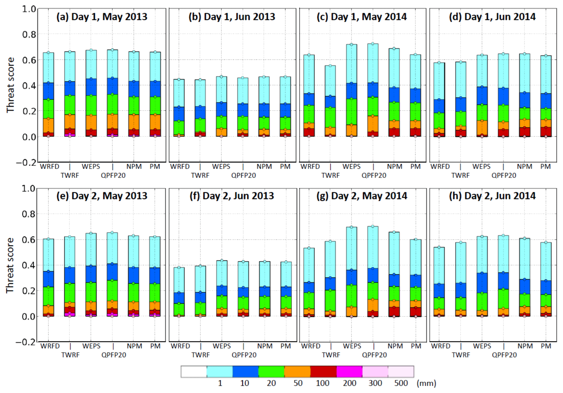
Figure 2 TSs of 0–24 h QPFs (day 1) for (a) May and (b) June of 2013 and (c) May and (d) June of 2014, respectively, at selected thresholds over 1–500 mm (per 24 h; scale at bottom) by two deterministic forecasts from WRF (WRFD) and the Typhoon WRF (TWRF) and four ensemble forecasts from the 20-member WRF Ensemble Prediction System: ensemble mean (WEPS), top 20 % (QPFP20), and WEPS employing the probability matching (PM) and new PM (NPM) techniques. (e–h) As in (a)–(d), but showing the TS of 24–48 h QPFs (day 2), respectively.

Wang (2015; hereafter referred to as W15) evaluated the QPFs within 3 d by a cloud-resolving model (CRM), the Cloud-Resolving Storm Simulator (CReSS; Tsuboki and Sakakibara, 2002, 2007), for all 15 typhoons that hit Taiwan in 2010–2012. With Δx=2.5 km, a grid size more comparable to research studies (e.g., Wang et al., 2005, 2011; 2013a, also Bryan et al., 2003; Done et al., 2004; Clark et al., 2007; Roberts and Lean, 2007), these deterministic forecasts showed superior performance in QPFs, with TSs of 0.38, 0.32, and 0.16 at thresholds of 100, 250, and 500 mm, respectively, for all typhoons on day 1 (0–24 h; cf. Fig. 13 of W15). Even on day 3 (48–72 h), the corresponding TSs are 0.21, 0.12, and 0.01. Thus, the accuracy of QPFs by this CRM over the thresholds of 100–500 mm is remarkably higher for typhoon rainfall in Taiwan.

Moreover, as summarized in Wang (2016), W15 found a strong positive dependency of categorical scores on overall rainfall amount (which represents event magnitude). That is, the larger the rain, the higher the scores and the better the model performs. For example, the TSs at the same thresholds (100, 250, and 500 mm) for the top five events (roughly top 5 %) in W15 on day 1 are 0.68, 0.49, and 0.24, respectively (Fig. 1 of Wang, 2016), all at least 1.5 times higher than their counterparts for all typhoons. An important implication of this finding is that the model QPFs for extreme events may not be accurately assessed through categorical statistics without proper classification to isolate them from ordinary events, and particularly not by taking the arithmetic mean of TSs of multiple forecasts. The study of W15 also predicts the dependency, as a fundamental property, to exist in other rainfall regimes. Therefore, the main purpose of this study is threefold: (1) to assess the ability of the 2.5 km CReSS in predicting Mei-yu rainfall at a higher resolution than before, especially for heavy to extreme rainfall events; (2) to clarify whether the dependency property in categorical scores also exists in the Mei-yu regime in Taiwan; and (3) to clarify whether the QPFs by CReSS are proven to be improved and why as well as where its strength lies.

In Sect. 2, the model, data, and methodology are described. In Sect. 3, the overall scores of QPFs for groups with different event magnitudes are presented and compared with previous results. Then in Sect. 4, examples are selected to illustrate how the CRM performs in real-time forecasts and where its strength lies. Aspects related to the dependency property are further discussed in Sect. 5, and our conclusions are given in Sect. 6.

2 Data and methodology

2.1 The CReSS model and its forecasts

The CReSS model is a non-hydrostatic, compressible CRM with a single domain without intermediate nesting (Tsuboki and Sakakibara, 2002, 2007), and it has been used for weather forecasts in Taiwan since 2006 (http://cressfcst.es.ntnu.edu.tw/, last access: January 2022; W15; Wang et al., 2013b, 2016a). Starting from July 2010, a grid size of 2.5 km is utilized, with a domain of 1500×1200 km² since May 2012 (Fig. 1a and Table 1). In CReSS, cloud formation, development, and all related processes are explicitly treated using a bulk cold-rain microphysical scheme with six species (Lin et al., 1983; Cotton et al., 1986; Murakami, 1990; Ikawa and Saito, 1991; Murakami et al., 1994): vapor, cloud water, cloud ice, rain, snow, and graupel (Table 1). Thus, no cumulus (or shallow convection) parameterization is used. Other sub-grid-scale processes parameterized in the model include turbulent mixing in the planetary boundary layer with a 1.5-order closure (Deardorff, 1980; Tsuboki and Sakakibara, 2007) as well as surface radiation and momentum and energy fluxes (Kondo, 1976; Louis et al., 1982; Segami et al., 1989). These physical options are identical to W15 and also given in Table 1.

Table 1 The basic configuration, initial/boundary conditions (IC/BCs), and physical packages of the 2.5 km CReSS used for real-time operation in 2012–2014. ^* The vertical grid spacing of CReSS is stretched (smallest at bottom), and the averaged spacing is given in the parentheses.

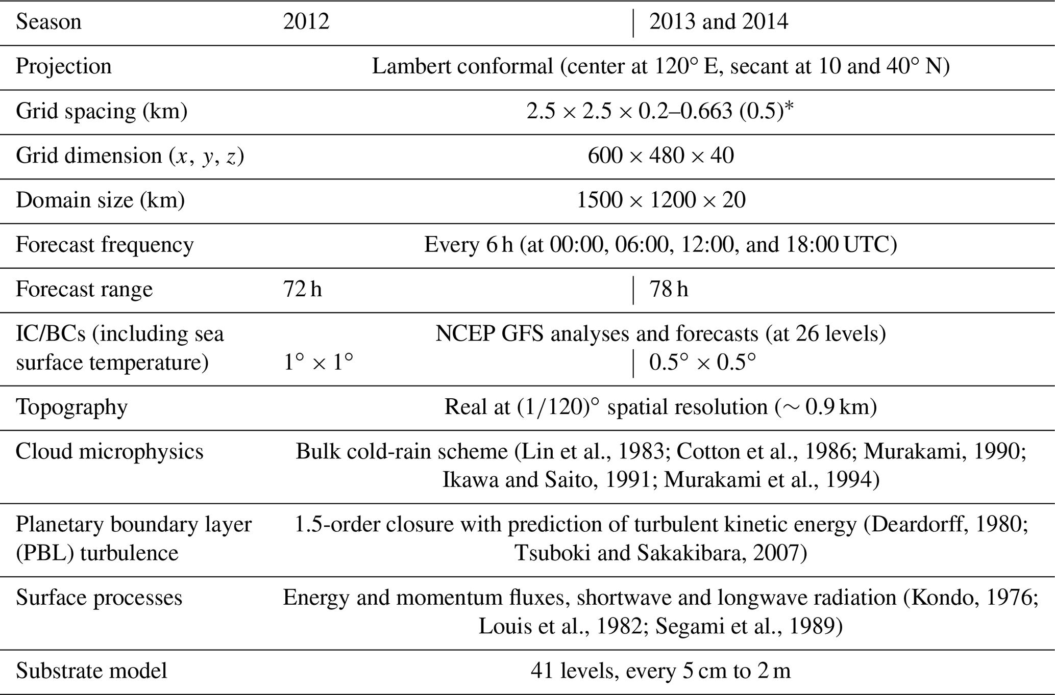
The operational analyses and forecasts by the Global Forecasting System (GFS; Kanamitsu, 1989; Kalnay et al., 1990; Moorthi et al., 2001; Kleist et al., 2009) of the National Centers for Environmental Prediction (NCEP), produced every 6 h (at 26 levels), were used as initial and boundary conditions (IC/BCs) for CReSS (Table 1). The CReSS model is also run four times a day, each out to 72 h (now 78 h). At the lower boundary, terrain data at 30^′′ resolution (roughly 900 m) and the NCEP analyzed sea surface temperature are also provided. With its limited domain size, the atmospheric evolution in CReSS is forced by the NCEP forecasts, especially at longer ranges. Note that since 2013, the IC/BCs from the GFS have increased the resolution from $\mathrm{1}{}^{\circ }\times \mathrm{1}{}^{\circ }$ to $\mathrm{0.5}{}^{\circ }\times \mathrm{0.5}{}^{\circ }$, but all other settings are kept the same during our study period (Table 1).

2.2 Data

The observational data used include synoptic weather maps from the CWB, the vertical maximum indicator reflectivity composites every 30 min from land-based radars, and hourly rainfall data from about 440 gauges in Taiwan for QPF verification (Fig. 1b). Along with NCEP gridded final analyses (on a $\mathrm{1}{}^{\circ }\times \mathrm{1}{}^{\circ }$ grid), the weather maps are used to identify and synthesize the occurrence of favorable factors to heavy rainfall among events with different magnitude (to be described in Sect. 2.3). For selected heavy-rainfall cases, the radar composites are compared with the CReSS forecasts to assess the quality of the QPFs in Sect. 4.

2.3 Verification period classification

In this study, objective categorical statistics (e.g., Schaefer, 1990; Wilks, 2011) are used to verify QPFs mainly because (1) the ability of models to predict the heavy rainfall at the correct location is imperative in Taiwan since its primary hazards are landslides and floods, and (2) our results can be easily compared with earlier studies. Here, 24 h QPFs are chosen because (1) the bulk rainfall accumulation from Mei-yu events, as for typhoons, is our main concern rather than the rain over shorter periods, especially at longer ranges (days 2–3), and (2) the issue of double penalty on high-resolution QPFs (e.g., Ebert and McBride, 2000) is less serious using a longer accumulation period. Although the CReSS forecasts are made four times a day, only those from 00:00 and 12:00 UTC are evaluated in this study.

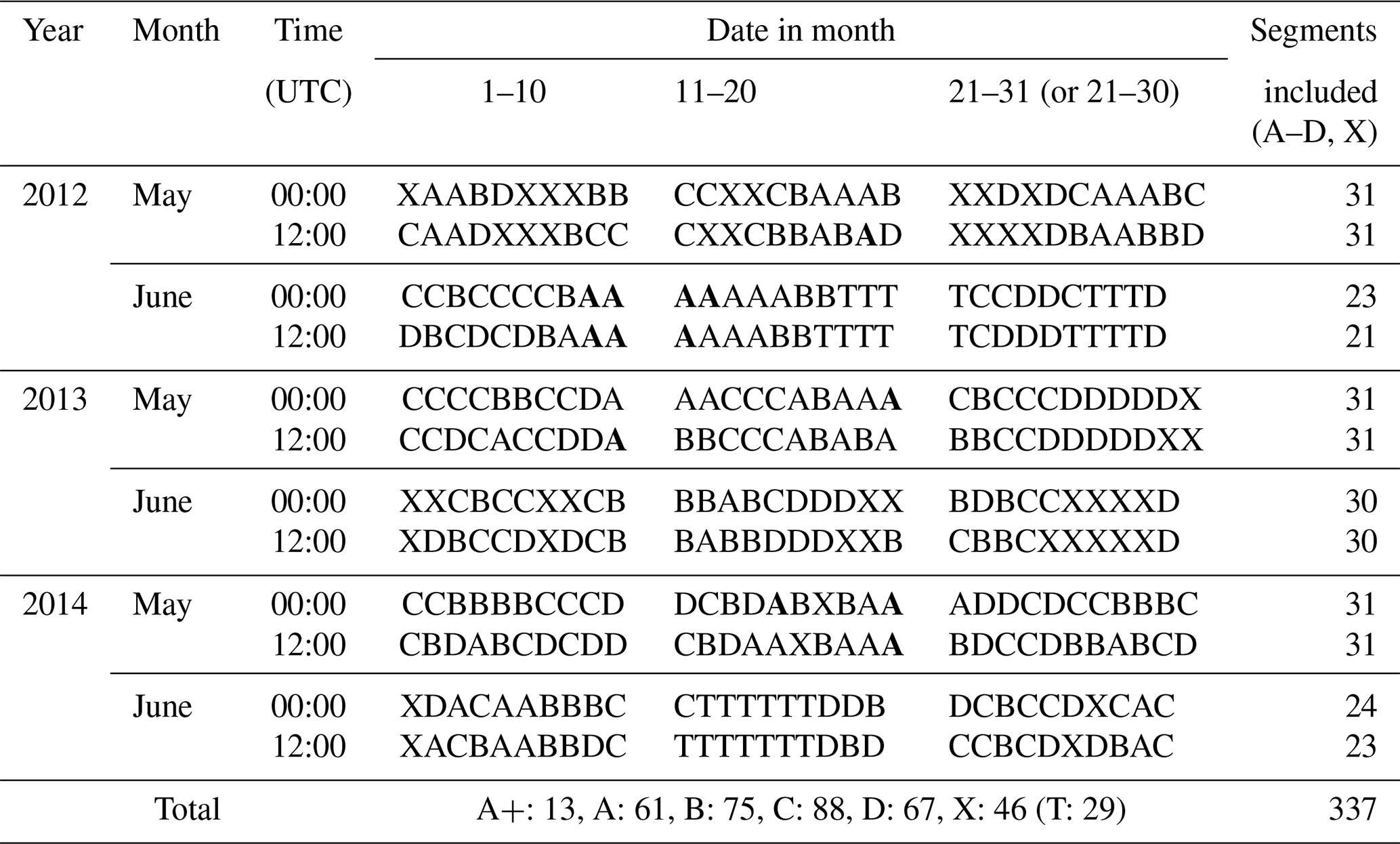
A total of 366 target segments (00:00–24:00 and 12:00–12:00 UTC) in May–June 2012–2014 are classified into several groups based on the observed rainfall using the following criteria, as summarized in Table 2. Groups A, B, C, and D are those periods with at least 10 % of rain gauges reaching 50, 25–50, 10–25, and 1–10 mm, respectively, while group X is the remaining periods with little or no rain. The full classification results (Table 3) give a total of 337 segments, excluding those under typhoon influence. Groups A–D individually account for about 18 %–26 % and are comparable in sample size, while the driest group, group X, is about 14 % (Tables 2 and 3). These five groups are exclusive to each other, and the results without classification are referred to as the “all” group. From group A, a subset of A+ that has ≥10 % of sites reaching 130 mm is identified and represents the rainiest 4 % of events in our sample with the highest hazard potential. The spatial distribution of mean Mei-yu rainfall per season in 2012–2014, with a peak amount of about 1700 mm, is shown in Fig. 3 and resembles the climatology (e.g., Yeh and Chen, 1998; Chien and Jou, 2004; Chi, 2006; Wang et al., 2017).

Table 2 The classification criteria using (at least) 10 % of rain gauges with highest 24 h accumulated rainfall (00:00–24:00 or 12:00–12:00 UTC) over Taiwan and the results in the number of 24 h segments (and percentage) and total points (sites) of $H+M+\mathrm{FA}$ at selected rainfall thresholds (mm) for the different groups. During the Mei-yu seasons of 2012–2014, the total N is 148 776, and on average there are 442 rain gauges per segment. The points of $H+M+\mathrm{FA}$ are based on the statistics of day − 1 (0–24 h) QPFs, and N is also given (with no threshold).

Table 3 The full classification result for all the 24 h verification periods during the three Mei-yu seasons of 2012–2014. For each month, the first (second) row gives the results of 00:00–24:00 (12:00–12:00) UTC. While the groups of A–D and X are denoted by their corresponding letter, a bold A indicates group A+ (a subset of A), and T marks the periods influenced by tropical cyclones and thus excluded from study.

2.4 Categorical measures of model QPFs

As mentioned, the 24 h QPFs by CReSS are verified against the rain gauge data, at three different ranges of 0–24, 24–48, and 48–72 h (days 1–3). For this purpose, objective scores computed from the standard 2×2 contingency table (or the categorical matrix) at a wide range of 14 thresholds from 0.05 to 750 mm are adopted. These measures include the TS (also called critical success index), bias score (BS), probability of detection (POD), and false alarm ratio (FAR), respectively defined as

$$\begin{array}{}\text{(1)}& {\displaystyle }& {\displaystyle }\mathrm{TS}=H/(H+M+\mathrm{FA}),\text{(2)}& {\displaystyle }& {\displaystyle }\mathrm{BS}=(H+\mathrm{FA})/(H+M)=F/O,\text{(3)}& {\displaystyle }& {\displaystyle }\mathrm{POD}=H/(H+M)=H/O,\mathrm{and}\text{(4)}& {\displaystyle }& {\displaystyle }\mathrm{FAR}=\mathrm{FA}/(H+\mathrm{FA})=\mathrm{FA}/F,\end{array}$$

where H, M, and FA are the counts of hits (both observed and predicted), misses (observed but not predicted), and false alarms (predicted but not observed), respectively, among a total number of N verification points (e.g., Schaefer, 1990; Wilks, 2011; Ebert et al., 2003; Barnes et al., 2009). Here, $N=H+M+\mathrm{FA}+\mathrm{CN}$, where CN is the correct negatives (neither observed nor predicted), and the total counts in observation (O) and forecast (F) are simply $O=H+M$ and $F=H+\mathrm{FA}$. The values of TS, POD, and FAR are all bounded by 0 and 1, and the higher (lower) the better for TS and POD (FAR). For BS, its value can vary from 0 to ∞ (or N−1 in practice), but unity is the most ideal and implies no bias. Also, BS $>(<)$ 1 implies overestimation (underestimation) of the events. By interpolating the model QPFs onto the gauge sites that serve as verification points (i.e., N≈440 per segment) using the bi-linear method, the counts of H, M, FA, and CN at any given threshold can be easily obtained for each segment. Although the density of rain gauges varies to some extent (roughly every 5–10 km in the plains and ≥10–20 km in the mountains; cf. Fig. 1b), their weights are assumed equal (e.g., Wang, 2014). For any group (e.g., A+) at a given threshold, the scores are obtained from a single 2×2 table that combines the entries from all segments so that the sample sizes are maximized (cf. Table 2; e.g., W15). This practice also remedies the issue of sampling inhomogeneity and increases the stability of results, especially toward the high thresholds, as long as the points involved in the matrix are not too few in number (cf. Table 2). Since neither the observation nor the forecast ever reached 750 mm (per 24 h) during the study period, results for 13 thresholds from 0.05 up to 500 mm (the next highest threshold) are presented in later sections. Also, only 24 h QPFs are evaluated in the current study. Except for the categorical matrix, subjective visual verification is also used in the selected examples (Sect. 4).

Figure 3 Spatial distribution of mean total rainfall (mm) per Mei-yu season (1 May through 30 June) in 2012–2014. The cities of Taipei and Kaohsiung are marked.

3 Mei-yu QPFs in 2012–2014

3.1 Overall performance by the 2.5 km CReSS

Following the method described above, the categorical matrices across the thresholds are obtained, and the overall ability of CReSS in Mei-yu QPFs during 2012–2014 is shown in Fig. 4 using the performance diagram. Proposed by Roebber (2009), the diagram uses the success ratio ($\mathrm{SR}=\mathrm{1}-\mathrm{FAR}=H/F$) and POD as its two axes and can also depict the TS (gray curved isopleths, higher toward upper right) and BS (dotted brown lines) simultaneously. In Fig. 4, the scores from forecasts at both 00:00 and 12:00 UTC for segments (of 24 h) in groups A+, A to D, and all periods (A–D plus X; cf. Table 2) at 13 thresholds are shown for ranges of day 1, 2, and 3, respectively. The “all” group (black) shows the overall accuracy for all Mei-yu rainfall without classification, and its TS for day − 1 QPFs decreases slowly from 0.6 at 0.05 mm to 0.18 at 100 mm, 0.15 at 250 mm, and 0.09 at 500 mm (Fig. 4a). Over heavy-rainfall thresholds ≥ 160 mm, the TSs of 0.09–0.16 are considerably higher than those reviewed in Sect. 1. Even on day 2, the TSs remain at 0.11 to 0.06 over 160–500 mm and above 0.03 up to 350 mm on day 3 (Fig. 4c and e).

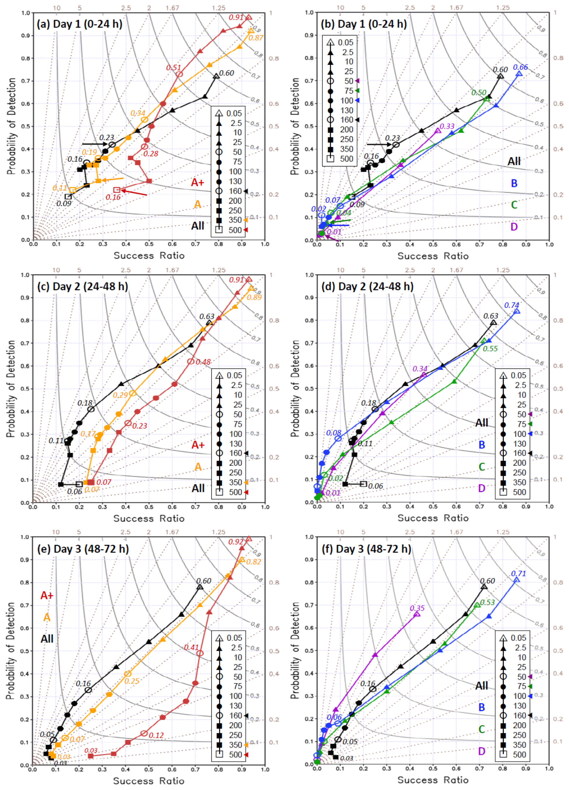
Figure 4 Performance diagrams of 24 h QPFs for (a, b) day 1 (0–24 h), (c, d) day 2 (24–48 h), and (e, f) day 3 (48–72 h) by the 2.5 km CReSS at 13 rainfall thresholds (inserts) from 0.05 to 500 mm during three Mei-yu seasons (May–June) in 2012–2014 in Taiwan. Results for groups A+, A, and “all” (“all”, B, C, and D) are plotted in the left (right) column with different colors. TS values are labeled at fixed thresholds of 0.05, 50, 160, and 500 mm (open symbols) or selected endpoints (smaller fonts), and data points with TS = 0 at high thresholds are omitted. For each group, the threshold where the observed rain area size ($O/N$) falls below 1 % is labeled in the insert and also marked by an arrow in (a, b).

When all segments are stratified by the observed event magnitude, the TSs are higher and the skill better for larger events than smaller ones, following the order of A+ then A to D for all thresholds at all three ranges without any exception (Fig. 4), while each individual curve mostly decreases with threshold when rain areas reduce in size (as shown in Fig. 5). Thus, the positive dependency of categorical measures on rainfall amount is also strong and evident in Mei-yu QPFs in Taiwan, as predicted by W15. Linked to this dependency, the TSs for large events are also higher than those for the “all” group from the entire sample. For the most hazardous group, group A+, the TS on day 1 is 0.34 at 100 mm, 0.24 at 250 mm, and 0.16 at 500 mm (per 24 h; Fig. 4a). On days 2 and 3, the corresponding TSs are 0.32, 0.15, and 0.07 (Fig. 4c) and 0.25, 0.05, and 0.00 (Fig. 4e), respectively, all higher than their counterparts for the “all” group (except day 3 at 500 mm). Similar to some earlier studies (e.g., Chien et al., 2002, 2006; Chien and Jou, 2004; Yang et al., 2004) and based on experience, if the value of TS ≥ 0.15, perhaps somewhat arbitrary, is used to indicate some level of accuracy, then the QPFs by the 2.5 km CReSS can reach it all the way up to 500 mm (per 24 h) on day 1, 250 mm on day 2, and 130 mm on day 3. Also, for the  A+, A, and “all” groups, the TSs of day − 2 QPFs stay quite close to the values on day 1, and some are even identical, from low thresholds up to 200–250 mm. For day − 3 QPFs compared to day 2, the same is true up to about 130 mm (Fig. 4, left column). Such results that some skill of heavy-rainfall QPFs still exists on days 2–3 are very encouraging. On the other hand, at thresholds ≥ 50 mm, the model's ability for B–D events (Fig. 4, right column) is limited (TS ≤ 0.08) when the rain areas are relatively small (with $O/N\le \mathrm{6}$ %; Fig. 5), but as discussed in W15, this is not important due to low hazard potential.

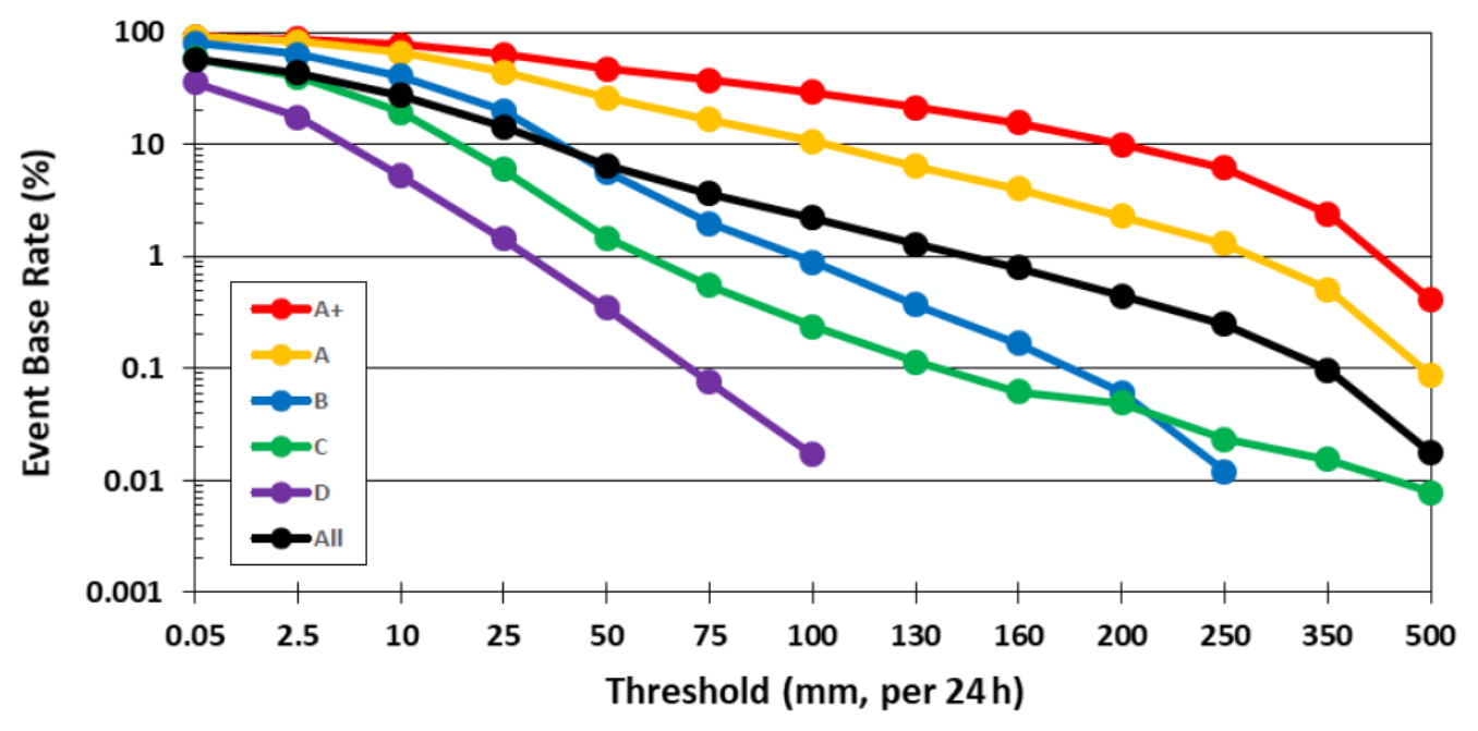
Figure 5 Observed rain area size or base rate ($O/N$, %) of 24 h rainfall (same for days 1–3) in logarithmic scale used to compute the scores in Fig. 4.

Another fairly subtle but important feature in Fig. 4 is that the TSs of the “all”, A, and A+ groups decrease only marginally for some heavy-rainfall thresholds, particularly on days 1–2, despite the reduction in rain area size (left column). Some examples include the TSs for group A+ over 100–350 mm on day 1 (drops from 0.34 to 0.21) and those for group A over the same thresholds on day 1 (from 0.23 to 0.15) and over 100–250 mm on day 2 (from 0.20 to 0.14). Even on day 3, the decrease in A and “all” curves from 160 to 350 mm is rather slow, although the TSs there are only 0.03–0.07 (Fig. 4e). Such a slow decline in TSs with thresholds indicates that in a relative sense, the model is more capable of producing hits toward the rainfall maxima, which occur more frequently in the mountains (cf. Figs. 1b and 3).

By definition, both POD and SR cannot be lower than the TS (cf. Eqs. 1, 3, and 4), and the ratio of POD $/$ SR equals the BS (thus, POD < SR if BS < 1 and vice versa). In Fig. 4, the PODs start at 0.05 mm from nearly perfect values of 0.98–0.99 for days 1–3 for group A+, at least 0.9 for A, and ≥0.72 for all segments (left column). For these three groups, the PODs at 250 mm remain at least 0.32 on day 1, 0.21 on day 2, and 0.05 on day 3. Like the TS, the POD for Mei-yu rainfall indeed decreases quite significantly with forecast range (lead time), particularly toward high thresholds, mainly due to error growth and the reduction in predictability. However, even on day 3, POD and TS can still reach 0.16 and 0.07 at 130 mm (for all segments), respectively. The SR values (and thus FAR) are again the best for group A+ and ≥0.36 across all thresholds on day 1, including 500 mm (Fig. 4a). On day 2, the SRs for A+ over 130–500 mm decrease but not by too much, and the values over 10–250 mm even increase on day 3 (Fig. 4c and e). Often, the SR for A+ is considerably higher than those for A and “all” events regardless of forecast range, particularly over heavy-rainfall thresholds. Overall, the model also produces higher POD and SR (i.e., lower FAR) for larger events compared to smaller ones at all thresholds and all three forecast ranges in Fig. 4, with only a few exceptions after close inspection. This indicates that the high-resolution CReSS not only produces larger rainfall for large rainfall events, which leads to a higher TSs, but also produces larger rainfall for small events, which leads to lower SR values. In summary, as for typhoon rainfall (W15), the 2.5 km CReSS is the most skillful in predicting the largest events in the Mei-yu season in Taiwan.

Next, the BS values are examined for over- and underprediction (i.e., above or below the diagonal line) in Fig. 4, where the threshold with $O/N$ falling below 1 % is marked to indicate values that might be potentially unstable and less meaningful. For day − 1 QPFs, the BSs for all segments suggest slight underprediction for low thresholds ≤ 10 mm (per 24 h) but some overprediction (BS ≈ 1.25–1.5) across 50–350 mm (Fig. 4a). In contrast, the model shows slight overprediction over 0.05–75 mm for the largest events of group A+ (with BSs up to 1.15) but underprediction toward higher thresholds, with the lowest BS of 0.52 at 350 mm. Mostly between the two curves mentioned above, the curve for group A stays closer to unity and is more ideal across nearly all thresholds (Fig. 4a). For B–D groups (Fig. 4b), their characteristics are similar to the “all” group, with BSs of 0.8–1.0 at low thresholds but generally some overprediction across higher thresholds. However, their BS values rarely exceed 2.5 unless the $O/N$ values drop to below 1 %. The situation for BSs between different groups remains similar on days 2 and 3 (Fig. 4c–f), and the over-forecasting across the middle thresholds in group A (at all ranges) can be confirmed to come mainly from groups B–D as groups A+ and A exhibit little or a much less tendency for overprediction there (Fig. 4).

Toward the longer ranges of days 2 and 3, the BS values in general become smaller, particularly for the larger groups (Fig. 4, left column). Thus, the overprediction in group A is reduced, and the underprediction in A+, which is the most important group, becomes more evident, especially toward the high thresholds (Fig. 4c and e). For example, the BS of day − 2 QPFs for A+ is ideal and ≥0.8 up to 200 mm but declines to about 0.35 at 500 mm, but it is already below 0.4 at 130 mm on day 3. This indicates that for larger events, the error growth with lead time in the model tends to become less rainy, as reflected in the decrease in BS. Thus, the probability of under-forecasting peak rainfall rises with lead time. For smaller events that do not produce much rainfall (i.e., B–D and X), a similar tendency does not exist or is weaker, and BS tends to be greater than unity. So, to say the least, one needs to practice caution in the interpretation of BS, which can also become unstable when $O/N$ approaches zero (which inevitably happens at certain thresholds).

3.2 Improvement in heavy-rainfall QPFs

To assess the improvement in heavy-rainfall QPFs in the Mei-yu season, our results in Fig. 4 are compared to Fig. 2 and those reviewed in Sect. 1. However, the differences in model resolution should be noted. Overall, the “all” curves in Fig. 4 indicate that the 2.5 km CReSS exhibits better skill than those reviewed in Sect. 1 (with Δx as fine as 5 km at most), especially at thresholds above 100 mm (e.g., TS = 0.15 at 250 mm and 0.09 at 500 mm for day 1). With even higher TSs for larger and more hazardous events (groups A and A+), the improvement of heavy-rainfall QPFs in the present study from earlier results is therefore quite clear and dramatic. The physical explanation is further elaborated and discussed later in Sect. 4.

4 Examples of model QPFs

Given the success of the CRM in its overall performance, some examples of CReSS forecasts are selected and presented in this section. The main goal here is twofold: (1) to illustrate how the model behaves and captures the rainfall in individual forecasts and thus (2) to identify where such a CRM has a better capability in QPFs and where it has limitations in Taiwan. Since our focus is on heavy rainfall, the event during 9–12 June 2012, the largest during our study period, is chosen for illustration.

The event of 9–12 June 2012 spanned 4 d and contributes more than half the segments in group A+ (7 in 13; cf. Table 3). In Fig. 6a, the observed 24 h rainfall distributions over Taiwan are shown every 12 h, from 12:00–12:00 UTC 8 June to 00:00–24:00 UTC 12 June 2012. Except for the first forecast period, all seven segments are qualified as A+, and five have a 24 h peak rainfall over 500 mm (those since 12:00 UTC 9 June). Three rainfall maxima from this lengthy event exist: over southern CMR, near the intersection of CMR and SMR in central Taiwan, and over northern Taiwan (Fig. 6a). The rain at the two mountain centers (cf. Fig. 1b) is much more persistent than that in northern Taiwan, which concentrated mainly over a 10 h period beginning 14:00 UTC 11 June (Wang et al., 2016b). The southwestern plains also received considerable rainfall, especially around 9 June (Fig. 6a).

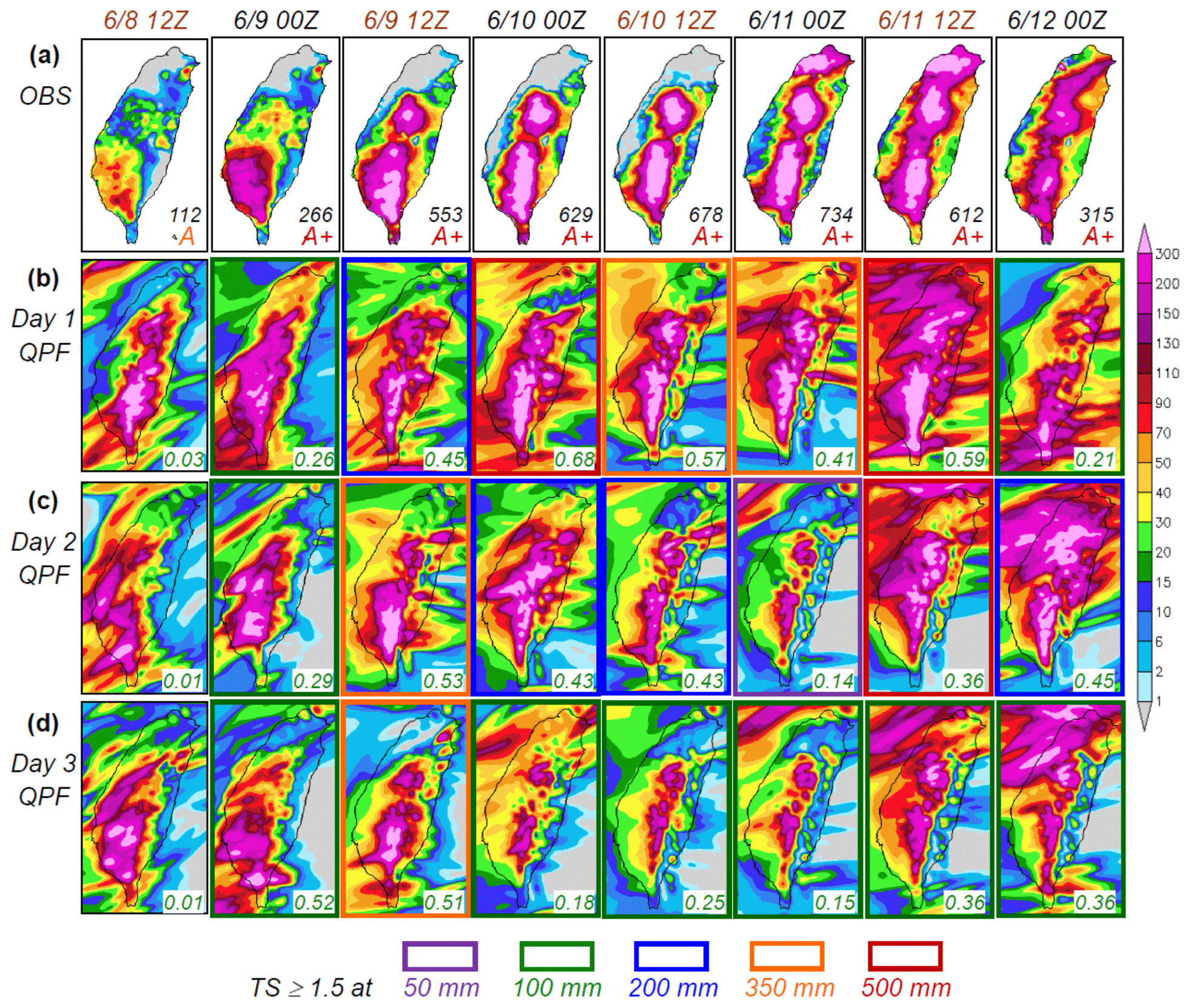
Figure 6 (a) The observed 24 h accumulated rainfall (mm; scale on the right) over Taiwan from 12:00 UTC 8 June to 00:00 UTC 13 June 2012, given every 12 h (from left to right), with the beginning time of accumulation (UTC) labeled on top (black for 00:00–24:00 UTC and brown for 12:00–12:00 UTC). (b) Day − 1 (0–24 h), (c) day − 2 (24–48 h), and (d) day − 3 (48–72 h) QPFs valid for the same 24 h periods as shown in (a) by the 2.5 km CReSS (starting at 00:00 or 12:00 UTC under black or brown headings, respectively). In (a), peak 24 h rainfall (mm) and classification group are labeled. In (b)–(d), thick boxes in purple, green, blue, orange, and scarlet denote forecasts having a TS ≥ 0.15 at the threshold of 50, 100, 200, 350, and 500 mm (per 24 h), respectively, and the TS at 100 mm is also given (lower right corner).

The 24 h QPFs produced by the 2.5 km CReSS (at 00:00 or 12:00 UTC) in real time targeting the same periods as in Fig. 6a in the range of days 1–3 are presented in Fig. 6b–d, with the general quality expressed by the TS at 100 mm (lower right corner inside panels) and thickened outline for TS ≥ 0.15 at the threshold of 50, 100, 200, 350, or 500 mm. The day − 1 QPFs (Fig. 6b) are made from the forecasts starting (with initial time t₀) at the time of the heading, while day − 2 (Fig. 6c) and day − 3 QPFs (Fig. 6d) are those made 24 and 48 h earlier (for the same target period), respectively. In Fig. 6, this extreme and long-lasting event was generally well captured by the model, especially on day 1, where the overall rainfall pattern and TS both tend to be better, as expected. The best day − 1 QPF is for 00:00–24:00 UTC 10 June (TS = 0.68 at 100 mm and 0.40 at 500 mm), followed by the one for 12:00 UTC 11–12 June (TS = 0.59 at 100 mm and 0.29 at 500 mm; columns 4 and 7, Fig. 6b). At longer ranges on days 2 and 3, the rainfall magnitudes produced over the mountains and southwestern plains are also comparable to observations, but the event starts somewhat earlier and becomes less rainy during 10–11 June, showing under-forecasting (Fig. 6c and d). As a result, the TSs for the segments starting at 12:00 UTC 8 June and during 10–11 June (columns 1 and 4–7) mostly increase from longer to shorter ranges, i.e., with better QPFs at later times. This relationship with range does not hold true for the other segments, among which the day − 3 and day − 2 QPFs for the period of 12:00 UTC 9–10 June (TS ≥ 0.51–0.53 at 100 mm and 0.20–0.31 at 350 mm) and the day − 2 QPF for 12:00 UTC 11–12 June (TS = 0.40 at 500 mm) are particularly impressive (columns 3 and 7). Compared to the rain over the terrain, the maximum across Taipei in northern Taiwan during 11–12 June was largely over lower and flatter regions (cf. Figs. 1b and 2) and more challenging for the model to predict at the right location (Fig. 6), an aspect that is further elaborated on later. Note, nevertheless, that since the mountain regions are the only places where rainfall amounts reach 300 mm in both the observations and the model (Fig. 6), any hits at and above this threshold occur in the mountains.

Figure 7 shows the TS and BS of day − 1 to day − 3 QPFs from the runs made at a series of initial times, including 12:00 UTC of 7–9 June and the next four from 00:00 UTC 10 June to 12:00 UTC 11 June (top to bottom), and our focus is mainly over the thresholds ≥ 100 mm. Inside the panels, the observed event base rate ($O/N$, i.e., rain area size, identical at the same threshold for the same target period) and the hit probability ($H/N$; note that $H/N\le O/N$) are given at selected points. Figure 7a–f provides some examples on how the model did in predicting the beginning of the event (cf. Fig. 6, columns 1–3). As mentioned, the day − 3 QPF made from 12:00 UTC 7 June (Fig. 7a and b, blue curves) and day − 2 QPF made 1 d later (Fig. 7c and d, red curves), both targeting 12:00 UTC 9–10 June, are of fairly high quality. With rain areas ($O/N$) occupying 31 %, 14 %, and just 2 % of Taiwan at 100, 200, and 350 mm, the day − 2 QPF in Fig. 7c, with BS ≈ 0.6–1.1 (Fig. 7d), yields TSs of 0.53–0.31 at these thresholds. For the day − 3 QPF with t₀ at 12:00 UTC 7 June, with less predicted rain and BS ≈ 0.3–0.6 (cf. Fig. 6d, column 3), the TSs are 0.51–0.2 (Fig. 7a and b). With a TS of at least 0.2 at 350 mm (an amount predicted only in the southern CMR), both QPFs (for 12:00 UTC 9–10 June) are quite good. Valid for periods with varying magnitude (B, A, and A+), the forecasts in Fig. 7a and b are also good examples to illustrate the dependency property (Fig. 4 and W15), where the rainfall amount apparently exhibits a larger influence on the scores than the forecast range. In Fig. 7e and f, the TS curves at the three ranges (all for A+ events) are closer.

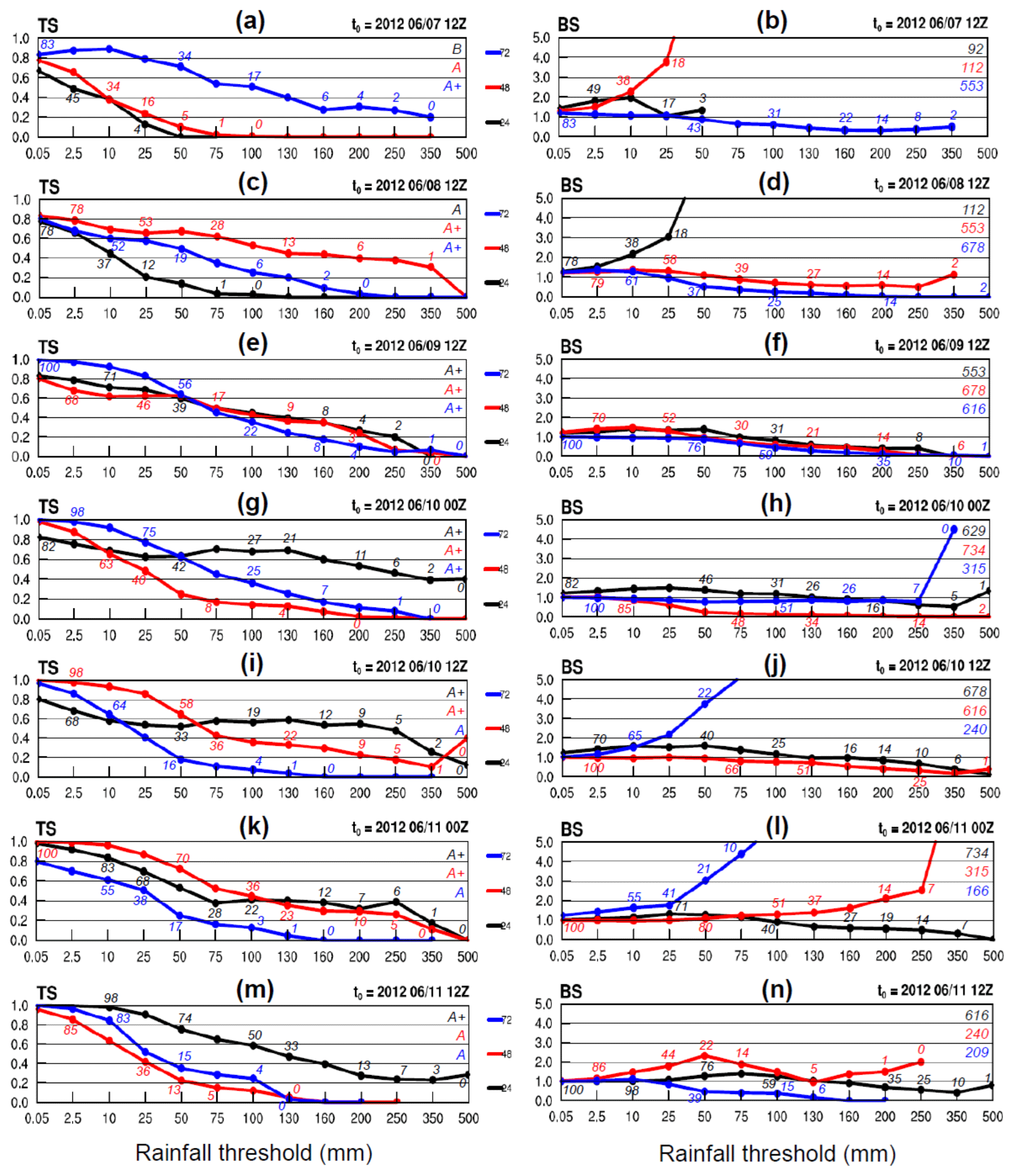
Figure 7 (a) TS and (b) BS of day − 1 (black), day − 2 (red), and day − 3 (blue) QPFs made at 12:00 UTC 7 June 2012 as a function of rainfall threshold (mm; per 24 h). The hit rate ($H/N$; %; rounded to integer) at selected points and the classification group for each day are labeled in the left panel (for TS). The observed base rate ($O/N$; %) and peak 24 h rainfall (mm) are labeled in the right panel (for BS). (c, d) to (m, n) As in (a, b), except for the QPFs made at (c, d) 12:00 UTC 8 June, (e, f) 12:00 UTC 9 June, (g, h) 00:00 UTC and (i, j) 12:00 UTC 10 June, and (k, l) 00:00 UTC and (m, n) 12:00 UTC 11 June 2012, respectively.

In Fig. 8, the actual forecast near Taiwan between 42 and 69 h, from the run made at 12:00 UTC 7 June, is compared with radar observations every 6 h to examine general rainfall locations. While a wind-shift line existed off eastern Taiwan, the surface Mei-yu front was well to the north, with prefrontal low-level southwesterly flow impinging on the island during this period (also Wang et al., 2016b). Active convection constantly developed over the mountains in central and southern Taiwan and moved from the upstream ocean into the southwestern plains, and this scenario was well captured by the 2.5 km CReSS (Fig. 8), yielding a high-quality QPF on day 3 despite some under-forecasting at thresholds ≥ 75 mm (cf. Fig. 7a and b).

Figure 8 (a, c, e, g, i, k) Radar reflectivity composite (dBZ; scale at bottom left) in the Taiwan area (width roughly 600 km) every 6 h from (a) 06:00 UTC 9 June to (k) 12:00 UTC 10 June 2012 (original plots provided by the CWB). (b, d, f, h, j, l) The CReSS forecast, starting from 12:00 UTC 7 June 2012, of sea-level pressure (hPa; every 1 hPa, over ocean only), surface wind (kn; barbs, at 10 m), terrain height at 1 and 2 km (gray contours), and hourly rainfall (mm; color, scale at bottom right) valid at the time or within 3 h of the radar composite as labeled – in UTC (forecast time in h) in lower (upper) right corner – over the same area. The thick dashed lines mark the position of surface frontal or wind-shift line, based on NCEP gridded analyses for the observation (outline of Taiwan also highlighted).

In the four following forecasts made on 10–11 June (Fig. 7g–n), the dependency on event magnitude exists, but the QPFs made for A+ periods tend to have higher TSs above 75–100 mm at the shorter ranges (Fig. 7g, i, and k). The TSs of these day − 1 QPFs can be as high as 0.48 at 250 mm and 0.40 at 500 mm. At 350–500 mm, such high TS occurs with $O/N$ below <10 % (or even only 1 %) and thus indicates remarkable model accuracy in predicting the peak rainfall at the correct location in the mountains in this event. Over thresholds ≥ 200 mm, BS values in Fig. 7 indicate that underprediction for this extreme event occurs much more often than overprediction, while they also tend to be closer to unity (with less under-forecasting) for QPFs achieving higher TSs. Consistent with Fig. 4, an overprediction is more likely to happen for smaller events (A or below), across low thresholds below 50 mm, and/or when the rain area becomes small. In Fig. 7, for example, BS ≥ 2 at high thresholds for the A+ group occurs only when $O/N$ approaches zero (Fig. 7h and n), with the only exception in Fig. 7l on day 2. Overall, the model does not have a tendency to overpredict such a large event (cf. Fig. 6).

The forecasts on days 1–2 produced by the run starting at 12:00 UTC 10 June are compared with radar observations in Fig. 9. Together with Fig. 8, the radar panels cover the wettest 72 h (06:00 UTC 9–12 June) of the entire event. During day 1 (Fig. 9a–h), the scenario remains similar to Fig. 8, and the model again was able to capture the mountain rainfall. The convection moving in from the Taiwan Strait, however, was too active, and the rain along the western coast on day 1 was overpredicted with BSs ≈ 1.2–1.6 from 0.05 up to 100 mm (cf. Fig. 7j). Note that in Fig. 7, some overprediction across low thresholds can also exist for group A+ and lowers the TS, which otherwise can often exceed 0.8 at and below 25 mm. In any case, the model's performance over the low thresholds is of secondary importance.

Figure 9 As in Fig. 8, but showing (a, c, e, g, i, k, m, o) radar reflectivity composite (dBZ) at (a) 14:00 UTC 10 June and every 6 h from (c) 18:00 UTC 10 June to (o) 06:00 UTC 12 June 2012 and (b, d, f, h, j, l, n, p) the CReSS forecast, starting from 12:00 UTC 10 June 2012, of sea-level pressure (hPa), surface wind (kn), and hourly rainfall (mm) valid at the time or within up to 8 h (towards the end) of the radar composite (as labeled).

Since 12:00 UTC 11 June, the Mei-yu front gradually approached northern Taiwan, and its western section moved rapidly across the island after about 00:00 UTC 12 June (Fig. 9i–p). Studied by Wang et al. (2016b), the heavy rainfall in northern Taiwan (during 14:00-24:00 UTC) was caused by quasi-linear convection that developed south of the front (Fig. 9i, k, and m), along a convergence zone between the low-level flow blocked and deflected by Taiwan's topography and unblocked flow further to the northwest (but still prefrontal) in the environment (e.g., Li and Chen, 1998; Yeh and Chen, 2002; Chen et al., 2005; Wang et al., 2005). In the model forecast, with apparent errors in the position and moving speed of the front (Fig. 9i–p), it is highly challenging to produce a similar system at the correct location and time even when the overall scenario surrounding northern Taiwan is reasonably predicted. In the simulation of Wang et al. (2016b), the rainbands cannot be fully captured even with a finer grid of Δx=1.5 km and the NCEP final analyses as IC/BCs. Likely mainly linked to the IC/BCs, the position error in the front in this case is still a major error source for the rainfall associated with the front. Thus, although the model did indicate a real possibility of heavy rainfall in northern Taiwan in Fig. 9, the high TS of 0.4 at 500 mm on day 2 (Fig. 7i) came from the mountains, where the rainfall prediction is clearly more accurate (cf. Fig. 6a and c, column 7), consistent with Walser and Schär (2004). Of course, the day − 1 QPF with $t_{\mathrm{0}}=\mathrm{12}:\mathrm{00}$ UTC 11 June performed better in northern Taiwan than our example, but the goal here is to illustrate the relatively high accuracy to predict heavy rainfall phase-locked to the topography versus the low accuracy for rainfall produced by transient systems over low-lying plains.

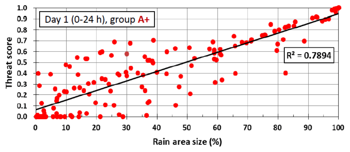
Figure 10 Scatterplot of TS versus observed rain area size (%) from day − 1 QPFs for group A+ from 0 % to 100 % (from high to low rainfall threshold). The squared correlation coefficient (R²) is given.

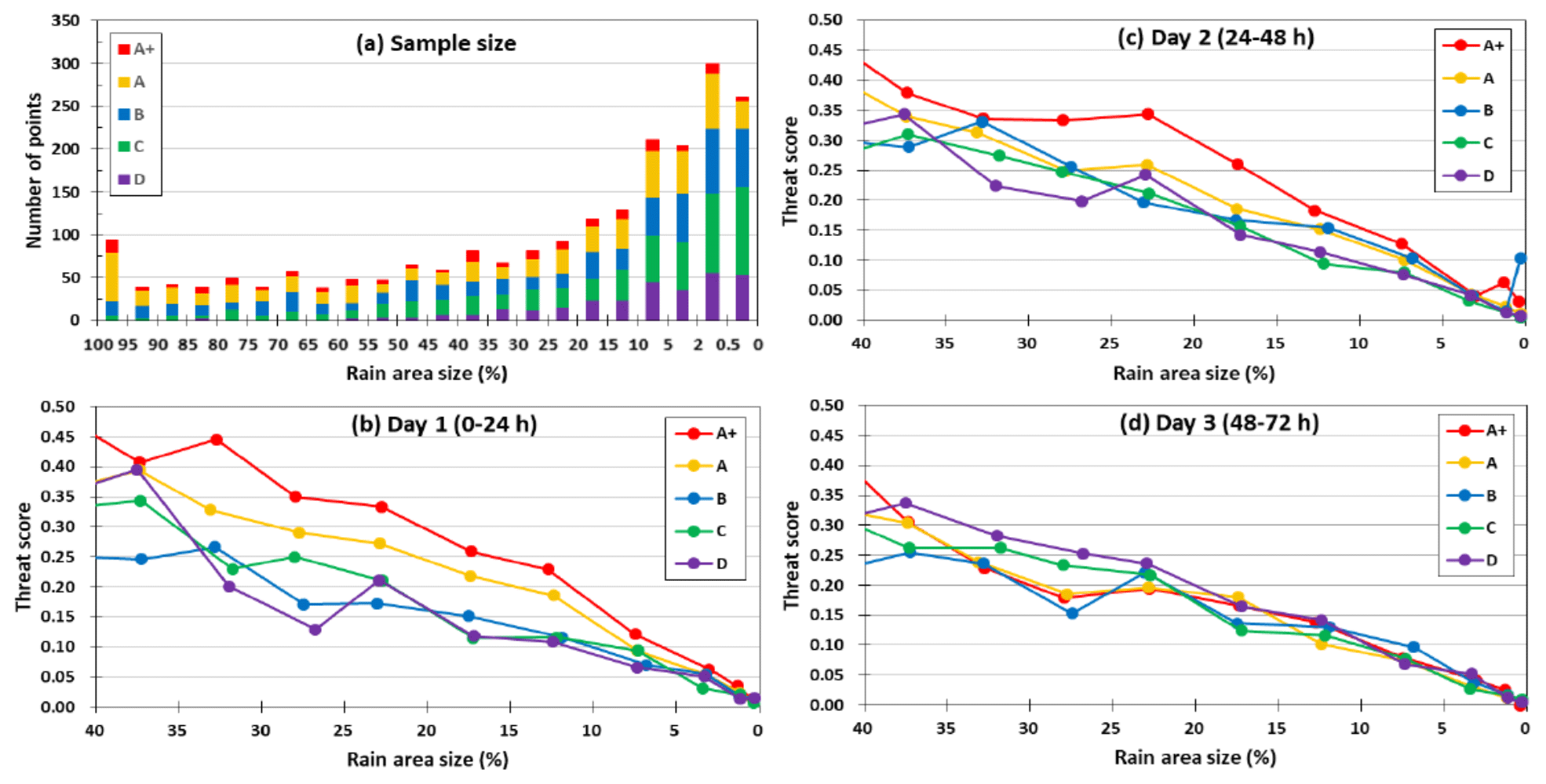
Figure 11 (a) The distribution of data points in the bins of observed rain area size (%; every 5 % from 100 % to 5 %, then 2 %–5 %, 0.5 %–2 %, and <0.5 %; same for days 1–3) among groups A+ and A to D. (b–d) The TS of 24 h QPFs for (b) day 1 to (d) day 3, respectively, as a function of observed rain area size between 40 % and 0 %.

The above example, together with other cases including those on 20 May 2013 and 20–21 May 2014, (cf. Table 3, not shown), suggests a lower accuracy and a more challenging task for model QPFs to capture the heavy rainfall produced by transient systems often in close association with the Mei-yu front compared to topographic rainfall in Taiwan. Even though the overall scenario is reasonably and realistically predicted (cf. Figs. 8 and 9), some position errors on the Mei-yu front are almost inevitable, and the intrinsic predictability can limit the accuracy of the QPF (e.g., Hochman et al., 2021). Also, for such rainfall caused by transient systems, categorical statistics are known to be less effective in verifying model QPFs (e.g., Davis et al., 2006; Wernli et al., 2008; Gilleland et al., 2010). However, for the quasi-stationary, phase-locked rainfall over the topography in the majority of large events (in both Mei-yu and typhoon seasons; e.g., Chang et al., 1993; Cheung et al., 2008) in Taiwan, they are still valid and useful, as shown herein. As model resolution increases, both the topography and deep convection can be better resolved, leading to improved QPFs over the terrain.

5 Dependency of categorical scores on event size

In Sect. 3, a positive dependency in categorical measures by CReSS, including TS, POD, and FAR, on rainfall amount is shown for the Mei-yu regime in Taiwan, as predicted. Also discussed in W15, this property arises mainly due to the positive correlation between the scores and rain area sizes, as illustrated in Fig. 10, with a correlation coefficient r=0.89 for the Mei-yu regime. However, to explore whether the model is indeed more skillful in predicting larger rainfall events, further analysis with the factor of rain area size removed is needed. Different from W15, our approach here is described below.

For each segment, the statistics (H, M, FA, and CN) at 13 fixed thresholds of 0.05–500 mm, each occurring at a certain $O/N$ (if the threshold is equal to or less than the observed peak amount), are known. The observed base rate (0 %–100 %) is divided into bins every 5 % except at 0 %–5 %, where it is subdivided into 0 %–0.5 %, 0.5 %–2 %, and 2 %–5 % to give more comparable sample size. For each group (A+ or A–D), the statistics are then summed for each bin regardless of their rainfall threshold. Thus, those in the same bin come from rain areas with similar sizes. In Fig. 11a, the distribution of total counts of thresholds across $O/N$ is plotted, and the larger events toward A+ are more capable of producing rain areas larger in size (say, ≥60 % of Taiwan). Also, the counts remain mostly around 50 for $O/N\ge \mathrm{40}$ %, then rise to 200–300 with $O/N\le \mathrm{10}$ %.

Due to fewer samples at larger $O/N$ values, the TSs for different groups (from a single 2×2 table for each bin) are presented only for $O/N\le \mathrm{40}$ % in Fig. 11b–d. While the scores for B–D are roughly the same, the TSs for A are clearly higher compared to those on day 1, and those for A+ are again higher compared to A on days 1 and 2 over most parts of this range, sometimes by 0.05–0.1, when the factor of rain area size is removed (Fig. 11b and c). On day 3 (Fig. 11d), however, the TSs for larger events (A+ and A) show no particular advantage. Therefore, similar to typhoons in W15, the 2.5 km CReSS is more skillful in predicting the larger Mei-yu events in Taiwan within 2 d over the heavy-rainfall area (again, mainly over the mountains).

The higher TSs and better skill for large events at $O/N$ within 40 % (Fig. 11) are most likely linked to the more favorable conditions at synoptic to meso-α scale, which the model is capable of capturing with higher accuracy (e.g., Walser and Schär, 2004). To briefly elaborate on this aspect, seven items on the checklist used by CWB forecasters in the Mei-yu season as a guidance to issue heavy-rainfall warning (e.g., Wang et al., 2012a) are selected, and their occurrence frequency, judged using surface weather maps and NCEP gridded analyses at the starting time of each 24 h period, is compiled for different groups. These items include (1) presence of surface Mei-yu front inside 20–28^∘ N, 118–124^∘ E; (2) Taipei (cf. Fig. 3) within 200 km south and 100 km north of the front; (3) Kaohsiung (cf. Fig. 3) within 200 km south of the front; (4) presence of a low-level jet (LLJ) inside 18–26^∘ N, 115–125^∘ E at 850 or 700 hPa; (5) presence of mesolow near Taiwan; (6) Taiwan inside a low-pressure zone; and (7) the mean sea-level pressure in Taiwan below 1005 hPa. The results (Fig. 12) indicate that among the seven items, an average of 4.15 items are met in group A+, and this figure gradually declines toward smaller groups, from 3.67 in A, 2.84 in B, and finally to only 0.87 in X. Thus, as expected, the synoptic- and meso-α-scale conditions tend to be more favorable in larger events, which in general also correspond to higher TS values (Figs. 3 and 11) in combination with the orographic forcing in Taiwan.

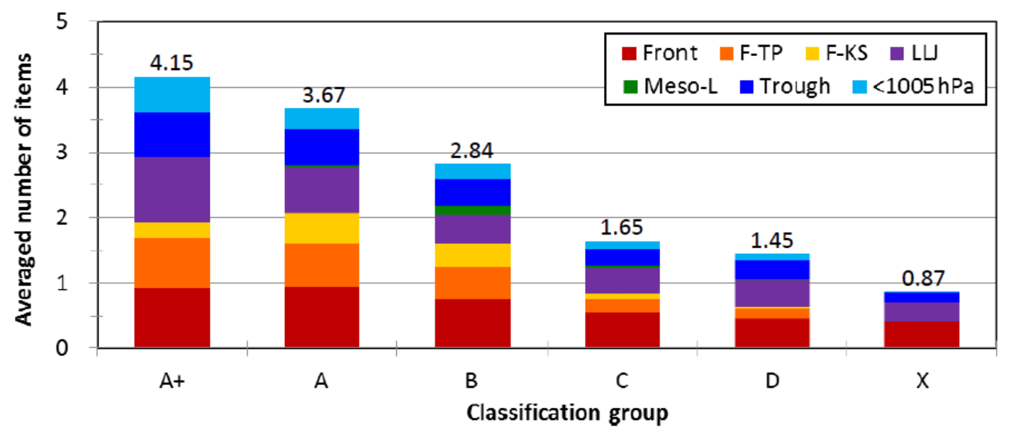
Figure 12 The average number of items met, among the seven items on the checklist, at the starting time of 24 h segments for different classification groups (from A+, A to D, and X), with the value labeled on top. Following the order (bottom to top), the seven items are presence of surface Mei-yu front (front), front near Taipei (F-TP), front near Kaohsiung (F-KS), presence of LLJ, mesolow (meso-L), Taiwan inside a low-pressure zone (trough), and the mean sea-level pressure lower than 1005 hPa (<1005 hPa), respectively. The items are plotted in different colors (see insert) to show their proportion.

6 Summary and concluding remarks

In this study, the QPFs at the ranges of 1–3 d by the 2.5 km CReSS during three Mei-yu seasons (May–June) in Taiwan of 2012–2014 are evaluated using categorical statistics, with an emphasis on heavy to extreme rainfall events (100–500 mm per 24 h). Overall, the TSs of day − 1 QPFs for all events (no classification) at thresholds of 100, 250, and 500 mm are 0.18, 0.15, and 0.09, respectively. Compared to previous and contemporary results from models at lower resolutions for the Mei-yu season in Taiwan, where the TSs are no higher than 0.1 at 100 mm and 0.02 at 250 mm and beyond (Sect. 1; e.g., Hsu et al., 2014; Li and Hong, 2014; Su et al., 2016; Huang et al., 2016), the results herein show considerable improvements by the 2.5 km CReSS, especially over the heavy-rainfall thresholds.

Moreover, the ability to represent the extreme and top events (group A+) in terms of the TS is much greater when a proper classification based on observed rain area size (i.e., event magnitude) is used. For the top 4 % and most hazardous Mei-yu events, the day − 1 QPFs have TSs of 0.34, 0.24, and 0.16, respectively. The QPFs for larger events also exhibit higher POD, lower FAR, and higher TS than smaller ones across nearly all thresholds at all ranges of days 1–3. Thus, the positive dependency of categorical scores on the overall rainfall amount also exists in the Mei-yu regime in Taiwan, as predicted by W15 (and Wang, 2016).

For a selected case study, the improvement by the 2.5 km CReSS in Taiwan is shown to lie in an improved ability to capture the phase-locked topographic rainfall at its correct location in larger events at heavy-rainfall thresholds. For rainfall in the mountains, the QPFs tend to be more accurate as the CRM can better resolve both the terrain and convection (e.g., Walser and Schär, 2004; Roberts and Lean, 2007). In contrast, the accuracy of QPFs for concentrated rainfall caused by transient systems (such as frontal squall lines) could not be demonstrated, probably due to the difficulty of predicting at the correct time and location owing to nonlinearity, even though a realistic scenario is produced. Overall, the high-resolution models showed a higher QPF accuracy in categorical statistics for extreme events than coarser-resolution models over the geographic region of Taiwan, as demonstrated here (and in W15). Such QPFs can be helpful for hazard preparation and mitigation.