the Creative Commons Attribution 4.0 License.
the Creative Commons Attribution 4.0 License.
 | 14 Jun 2022
Data-driven automated predictions of the avalanche danger level for dry-snow conditions in Switzerland
Cristina Pérez-Guillén
Frank Techel
Martin Hendrick
Michele Volpi
Alec van Herwijnen
Tasko Olevski
Guillaume Obozinski
Fernando Pérez-Cruz
Jürg Schweizer
Even today, the assessment of avalanche danger is by and large a subjective yet data-based decision-making process. Human experts analyse heterogeneous data volumes, diverse in scale, and conclude on the avalanche scenario based on their experience. Nowadays, modern machine learning methods and the rise in computing power in combination with physical snow cover modelling open up new possibilities for developing decision support tools for operational avalanche forecasting. Therefore, we developed a fully data-driven approach to assess the regional avalanche danger level, the key component in public avalanche forecasts, for dry-snow conditions in the Swiss Alps. Using a large data set of more than 20 years of meteorological data measured by a network of automated weather stations, which are located at the elevation of potential avalanche starting zones, and snow cover simulations driven with these input weather data, we trained two random forest (RF) classifiers. The first classifier (RF 1) was trained relying on the forecast danger levels published in the official Swiss avalanche bulletin. To reduce the uncertainty resulting from using the forecast danger level as target variable, we trained a second classifier (RF 2) that relies on a quality-controlled subset of danger level labels. We optimized the RF classifiers by selecting the best set of input features combining meteorological variables and features extracted from the simulated profiles. The accuracy of the models, i.e. the percentage of correct danger level predictions, ranged between 74 % and 76 % for RF 1 and between 72 % and 78 % for RF 2. We assessed the accuracy of forecasts with nowcast assessments of avalanche danger by well-trained observers. The performance of both models was similar to the agreement rate between forecast and nowcast assessments of the current experience-based Swiss avalanche forecasts (which is estimated to be 76 %). The models performed consistently well throughout the Swiss Alps, thus in different climatic regions, albeit with some regional differences. Our results suggest that the models may well have potential to become a valuable supplementary decision support tool for avalanche forecasters when assessing avalanche hazard.
- Article
(7948 KB) - Full-text XML
- Companion paper
-
Supplement
(52259 KB) - BibTeX
- EndNote


Avalanche forecasting, i.e. anticipating the probability of avalanche occurrence and the expected avalanche size in a given region (and time period) (Schweizer et al., 2020; Techel et al., 2020a), is crucial to ensure safety and mobility in avalanche-prone areas. Therefore, in many countries with snow-covered mountain regions, avalanche warning services regularly issue forecasts to inform the public and local authorities about the avalanche hazard. Even today, these forecasts are prepared by human experts. Avalanche forecasters analyse and interpret heterogeneous data volumes diverse in scale, such as meteorological observations and model output in combination with snow cover and snow instability data, covering a wide range of data qualities. Eventually, forecasters decide, by expert judgement, on the likely avalanche scenario according to guidelines such as the European Avalanche Danger Scale (EAWS, 2021a) or description of the typical avalanche problems (Statham et al., 2018; EAWS, 2021c). Hence, operational forecasting by and large still follows the approach described by LaChapelle (1980), despite the increasing relevance of modelling approaches (Morin et al., 2020).
A key component of public avalanche forecasts is the avalanche danger level, usually communicated according to a five-level, ordinal danger scale (EAWS, 2021a). The danger level summarizes avalanche conditions in a given region with regard to the snowpack stability, its frequency distribution, and the avalanche size (Techel et al., 2020a). Accurate danger level forecasts support recreationists and professionals in their decision-making process when mitigating avalanche risk. However, avalanche danger cannot be measured and hence is also not easily verified – and avalanche forecasting has even been described as an art based on experience and intuition (LaChapelle, 1980; Schweizer et al., 2003). To improve the quality and consistency of avalanche forecasts, various statistical models (see Dkengne Sielenou et al., 2021, for a recent review) and conceptual approaches have been developed. The latter, for instance, include a proposition for a structured workflow (Statham et al., 2018) and look-up tables (e.g. EAWS, 2017; Techel et al., 2020a), both aiding forecasters in the decision-making process of danger assessment.
A major challenge when developing or verifying statistical models, as well as avalanche forecasts in general, is the lack of a measurable target variable. Since avalanche occurrence seems a logical target variable, most of the previous approaches have focused on the estimation of avalanche activity using typical machine learning methods such as classification trees (Davis et al., 1999; Hendrikx et al., 2014; Baggi and Schweizer, 2009), nearest neighbours (Purves et al., 2003), support vector machines (Pozdnoukhov et al., 2008, 2011), and random forests (Mitterer and Schweizer, 2013; Möhle et al., 2014; Dreier et al., 2016; Dkengne Sielenou et al., 2021). To build and validate these models, a substantial number of avalanche data are required. However, avalanche catalogues are particularly uncertain and incomplete (Schweizer et al., 2020) since they rely on visual observations that are not always possible or are delayed; a practical solution is to use avalanche detection systems, but such data are still scarce and/or only locally available (e.g. Hendrikx et al., 2018; van Herwijnen et al., 2016; Heck et al., 2019; Mayer et al., 2020).
Apart from estimating avalanche activity, a few models have focused on automatically forecasting danger levels. Schweizer et al. (1992) prepared a data set for model development that included the verified danger level for the region of Davos. Based on these data, Schweizer et al. (1994) developed a hybrid expert system to assess the danger level, integrating symbolic learning with neuronal networks and using weather and snow cover data as input parameters for the model, which correctly classified about 70 % of the cases. A similar performance was achieved by Schweizer and Föhn (1996) using an expert system approach. Brabec and Meister (2001) trained and tested a nearest-neighbour algorithm to forecast danger levels for the entire Swiss Alps using manually observed snow and weather data from 60 stations. They reported a low overall accuracy of 52 %, probably due to the lack of input variables related to the snow cover stability. Combining different feature sets of simulated snow cover data and meteorological variables, Schirmer et al. (2009) compared the performance of several machine learning methods (e.g. classification trees, artificial neural networks, nearest-neighbour methods, support vector machines, and hidden Markov models) to predict the danger level in the region of Davos (Switzerland). Their best classifier was a nearest-neighbour model, including the avalanche danger level of the previous day as an additional input variable, that achieved a cross-validated accuracy of 73 %.
Despite many efforts, few of the previously developed models have been operationally applied due to lack of automated and real-time data, transferability to other regions, or snowpack stability input – all deficiencies that limited their utility for operational forecasting. Moreover, most models have used daily snow and weather data, manually observed at low elevations, that do not reflect avalanche conditions in the high Alpine environment. Today, ample data from automated weather stations and snow cover model outputs are available (Lehning et al., 1999). The quality and breadth of these data make them suitable for applying modern machine learning methods.
Therefore, our aim is to develop an effective data-driven approach to assess the regional avalanche danger level. An inherent characteristic of avalanche forecasts is that they are, at times, erroneous. In general, forecast accuracy is difficult to assess as avalanche danger cannot be measured and remains a matter of expert assessment even in hindsight (Föhn and Schweizer, 1995; Schweizer et al., 2003). Even though this target variable is hard to verify and susceptible to human biases and errors, the danger level is the key component of avalanche bulletins for communicating avalanche hazard to the public. We will focus on dry-snow conditions as dry-snow slab avalanches are the most prominent danger and develop a model that can be applied to all snow climate regions in the Swiss Alps and should have an accuracy comparable to the operational experienced-based forecast. We address avalanche prediction (in nowcast mode) as a supervised classification task that involves assigning a class label corresponding to the avalanche danger level to each set of meteorological and simulated snow cover data from an automatic weather station network located in Switzerland.
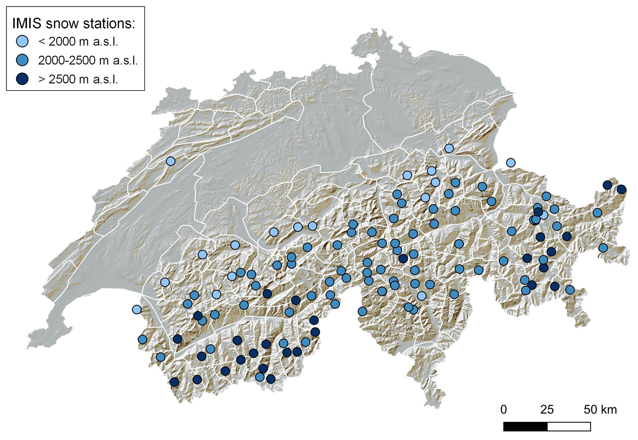
Figure 1Snow stations of the IMIS network (points) located throughout the Swiss Alps (one station in northeastern Jura region) and the warning regions (white contours) used to communicate avalanche danger in the public avalanche forecast. Stations are coloured according to their elevation: below 2000 m a.s.l., between 2000 and 2500 m a.s.l., and above 2500 m a.s.l.
We rely on more than 20 years of data, collected in the context of operational avalanche forecasting in the Swiss Alps, covering measured meteorological data and snow cover simulations (Sect. 2.1), as well as the regional danger level published in the avalanche forecasts (Sect. 2.2) and local assessments of avalanche danger provided by experienced observers (Sect. 2.3). The data cover the winters from 1997/98 to 2019/20.
2.1 Meteorological measurements and snow cover simulations
In Switzerland, a dense network of automatic weather stations (AWSs), located at the elevation of potential avalanche starting zones, provides real-time weather and snow data for avalanche hazard assessment. These data are used both by the Swiss national avalanche warning service for issuing the public avalanche forecast and by local authorities responsible for the safety of exposed settlements and infrastructure. This network, the Intercantonal Measurement and Information System (IMIS), was set up in 1996 with an initial set of 50 operational stations in the winter of 1997/98 (Lehning et al., 1999). It currently consists of 182 stations (2020), of which 124 are snow stations located in level terrain at locations sheltered from the wind (Fig. 1). About 15 % of the stations are situated at elevations between 1500 and 2000 m a.s.l., 61 % between 2000 and 2500 m a.s.l., and 24 % between 2500 and 3000 m a.s.l. The IMIS stations operate autonomously, and the data are transmitted every hour to a data server located at WSL Institute for Snow and Avalanche Research SLF (SLF) in Davos.
Based on the measurements provided by the AWSs, snow cover simulations with the 1D physically based, multi-layer model SNOWPACK (Lehning et al., 1999, 2002) are performed automatically throughout the winter, providing output for local and regional avalanche forecasting. The meteorological data are pre-processed (MeteoIO library; Bavay and Egger, 2014), filtering erroneous data and imputing missing data relying on temporal interpolation or on gap filling by spatially interpolating from neighbouring stations. The SNOWPACK model provides two types of output: (1) the pre-processed meteorological data and (2) the simulated snow stratigraphy data. For an overview of the SNOWPACK model, refer to Wever et al. (2014) and Morin et al. (2020). In this study, we extracted the flat-field snow cover simulations from the database used operationally for avalanche forecasting.
2.2 Avalanche forecast
The avalanche forecast is published by the national avalanche warning service at SLF. During the time period analysed, the forecast was published daily in winter – generally between early December and late April – at 17:00 LT (local time), valid until 17:00 LT the following day, for the whole area of the Swiss Alps (Fig. 2). In addition, since 2013, the forecast has been updated daily at 08:00 LT – between about mid-December and early April to mid-April. Furthermore, an avalanche forecast has also been published for the Jura Mountains since 2017 (Fig. 2).
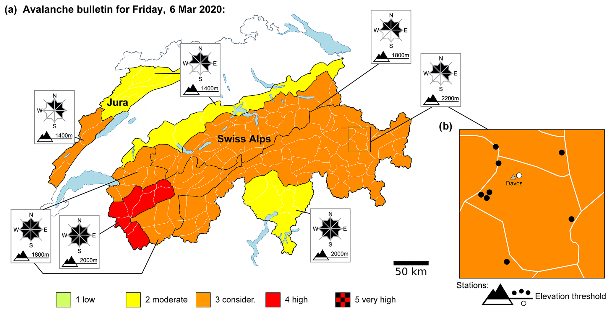
Figure 2(a) Map of the avalanche danger issued on Friday 6 March 2020 at 08:00 LT (local time). For each danger region (black contour lines), a danger level from 1-Low to 5-Very High and the critical elevations and slope aspects are graphically displayed. The white polygons show the 130 warning regions. (b) Close-up map of the warning region Davos, with the location of the IMIS stations (points). To develop the model, we filtered days and stations as a function of the critical forecast elevation (Sect. 3.3), with stations coloured black being above this elevation on this day (here 2200 m a.s.l.) and hence considered and the white station, located below this elevation, not considered.
The forecast domain of the Swiss Alps (about 26 000 km2) is split into 130 warning regions (status in 2020), with an average size of about 200 km2 (white polygon boundaries shown in Figs. 1 and 2). In the forecast, these warning regions are grouped according to the expected avalanche conditions into danger regions (black polygon boundaries shown in Fig. 2). For each of these danger regions, avalanche danger is summarized by a danger level; the aspects and elevations where the danger level is valid, together with one or several avalanche problems (since 2013); and a textual description of the danger situation. The danger level is assigned according to the five-level European Avalanche Danger Scale: 1-Low, 2-Moderate, 3-Considerable, 4-High, and 5-Very High (EAWS, 2021a).
2.3 Local nowcast of avalanche danger level
Specifically trained observers assess the avalanche danger in the field and transmit their estimate to the national avalanche warning service. Observers rate the current conditions for the area of their observations, for instance after a day of backcountry touring in the mountains. To do so, they are advised to consider their own observations as well as any other relevant information (Techel and Schweizer, 2017). For these local assessments of the avalanche danger level, the same definitions (EAWS, 2021a) and guidelines (e.g. EAWS, 2017, 2021b) are applied as for the regional forecast. These assessments, called local nowcasts, are used operationally during the production of the forecast, for instance, to detect deviations between the forecast of the previous day and the actually observed conditions.
We used the local nowcasts (1) to filter potentially erroneous forecasts when compiling a subset of danger levels as described in detail in Appendix A and (2) to discuss the model performance in light of the noise inherent in regional forecasts. These assessments are human judgements and thus rely on a similar approach to that followed by a forecaster when assigning a danger level. Techel (2020) compared danger level assessments in the same area and estimated the reliability as 0.9, which is a factor related to the agreement rate of pairs of local nowcast estimates between several observers within the same warning region.
We first defined and prepared the target variable, the danger level (Sect. 3.1). In the next step, we extracted relevant features describing meteorological and snow cover conditions (Sect. 3.2), before linking them to the regional danger levels (Sect. 3.3). Finally, we split the merged data sets for evaluating the performance of a machine learning algorithm (Sect. 3.4).
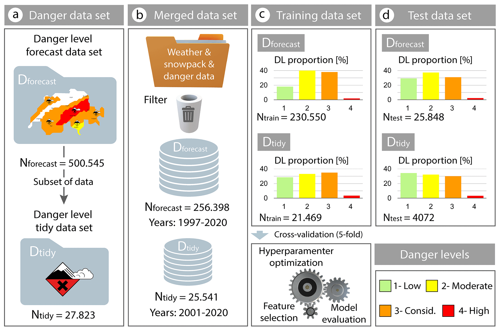
Figure 3Flowchart of the data set distributions and steps, including the raw data volume, the merged and filtered data set size, and the danger level distributions of the training and test sets. Two machine learning classifiers are trained using as labels (i) the forecast danger levels (Dforecast) in the public bulletin and (ii) a subset of tidy danger levels (Dtidy). An iterative process of hyperparameter tuning and feature selection using 5-fold cross-validation was conducted to select the best model.
3.1 Preparation of target variable
We considered two approaches to define the target variable: first, by simply relying on the forecast danger level (Sect. 3.1.1) and, second, by compiling a much smaller subset of “tidy” danger levels (Sect. 3.1.2). The first approach makes use of the entire database. However, this comes at the cost of potentially including a larger share of wrong labels. In contrast, the second approach uses higher-quality labelling, but the data volume is greatly reduced.
3.1.1 Target variable – forecast danger level (Dforecast) relating to dry-snow conditions
To train the machine learning algorithms, we rely on forecasts related to dry-snow conditions in the forecast domain of the Swiss Alps (Fig. 2). Whenever a morning forecast update was available, we considered this update. In this update, on average the forecast danger level is changed in less than 3 % of the cases (Techel and Schweizer, 2017). The focus on dry-snow conditions is motivated by the fact that both the meteorological factors and the mechanisms that lead to an avalanche release differ greatly between dry-snow and wet-snow avalanches. Furthermore, while danger level forecasts for dry-snow avalanche conditions are issued on a daily basis, forecasts for wet-snow avalanche conditions are only issued on days when the wet-snow avalanche danger is expected to exceed the dry-snow avalanche danger (SLF, 2020).
In total, this procedure resulted in a data set that included forecasts issued on 3820 d during the 23 winters between 11 November 1997 and 5 May 2020, with a total of 500 545 cases (Fig. 3a). We refer to this data set as Dforecast, which is used as ground truth data labelling. The distribution of danger levels is clearly imbalanced (top of Fig. 3c). The most frequent danger levels forecast in the Alps are danger levels 2-Moderate (41 %) and 3-Considerable (36 %), which jointly account for 77 % of the cases. Since danger level 5-Very High is rarely forecast (<0.1 %), we merged it with danger level 4-High (2.0 %).
3.1.2 Compilation of subset of tidy danger level (Dtidy)
Incorrect labels in the Dforecast data set are unavoidable as avalanche forecasts are sometimes erroneous due to inaccurate weather forecasts, variations in local weather and snowpack conditions, and human biases (McClung and Schaerer, 2006). In general, as avalanche forecasts are expert assessments, there is inherently noise (Kahneman et al., 2021). In terms of the target variable, these errors may manifest themselves in errors in the danger level, the elevation information indicated in the forecast, or the spatial extent of regions with a specific danger level. Furthermore, all of these elements are gradual in nature and not step-like as the danger level, the elevation band, and the delineation of the warning regions suggest. In the case of forecast danger levels in Switzerland, recent studies have estimated the accuracy of the forecast danger level. The agreement rate between local nowcast estimates of the avalanche danger with the forecast danger level was between about 75 % and 90 %, with a decreasing agreement rate with an increasing danger level (Techel and Schweizer, 2017; Techel, 2020). A particularly low accuracy (<70 %) was noted for forecasts issuing danger level 4-High (Techel, 2020). Furthermore, a strong tendency towards over-forecasting (by one level) has been noted, with forecasts rarely being lower compared to nowcast assessments of avalanche danger (e.g. Techel et al., 2020b).
To reduce some of the inherent noise, we compiled a subset of re-analysed danger levels, for which we were more certain that the issued danger level was correct. This should not be considered a verified danger level but simply a subset of danger levels, which presumably have a greater correspondence with actual avalanche conditions compared to simply using the forecast danger level. To compile this subset, we checked the forecast danger level Dforecast by considering additional pieces of evidence. For this, we relied on
-
observational data – for instance, danger level assessments (local assessments) provided by experienced observers after a day in the field (Sect. 2.3; Techel and Schweizer, 2017) or avalanche observations – and
-
the outcome from several verification studies (Schweizer et al., 2003; Schweizer, 2007; Bründl et al., 2019; Zweifel et al., 2019).
Thus, this data set is essentially a subset of Dforecast, containing cases of Dforecast which were either confirmed or validated following multiple pieces of evidence. Comparably few of these cases (5 %) were actually cases when the forecast danger level was corrected for the purpose of this study. These changes affected primarily days and regions when the forecast was either 4-High or 5-Very High or when the verified danger level was one of these two levels. We refer to this subset as tidy danger levels (Dtidy), which is also used as ground truth data labelling. A detailed description regarding the compilation of this data set is found in Appendix A.
Dtidy (N=25 541 cases in Fig. 3b) comprises about 10 % of the Dforecast data set (N=256 398 cases after filtering in Fig. 3b). In this subset, the distribution of the lower three danger levels is approximately balanced (about 30 % each, Fig. 3). Still, this subset contains comparably few cases of higher danger levels (4-High, 4.1 %; 5-Very High, 0.3 %). These two danger levels (4-High and 5-Very High) were again merged and labelled 4-High.
3.2 Feature engineering
The SNOWPACK simulations provide two different output files for each station: (i) time series of meteorological variables and (ii) simulated snow cover profiles. The first includes a combination of measurements (i.e. air temperature, relative humidity, snow height, or snow temperature) and derived parameters (i.e. height of new snow, outgoing and incoming long-wave radiation, and snow drift by wind). The snow profiles contain the simulated snow stratigraphy describing layers and their properties. Figure 4 shows an example of these data. A list of the 67 available weather and profile features is shown in Tables C1 and C2 (Appendix C).
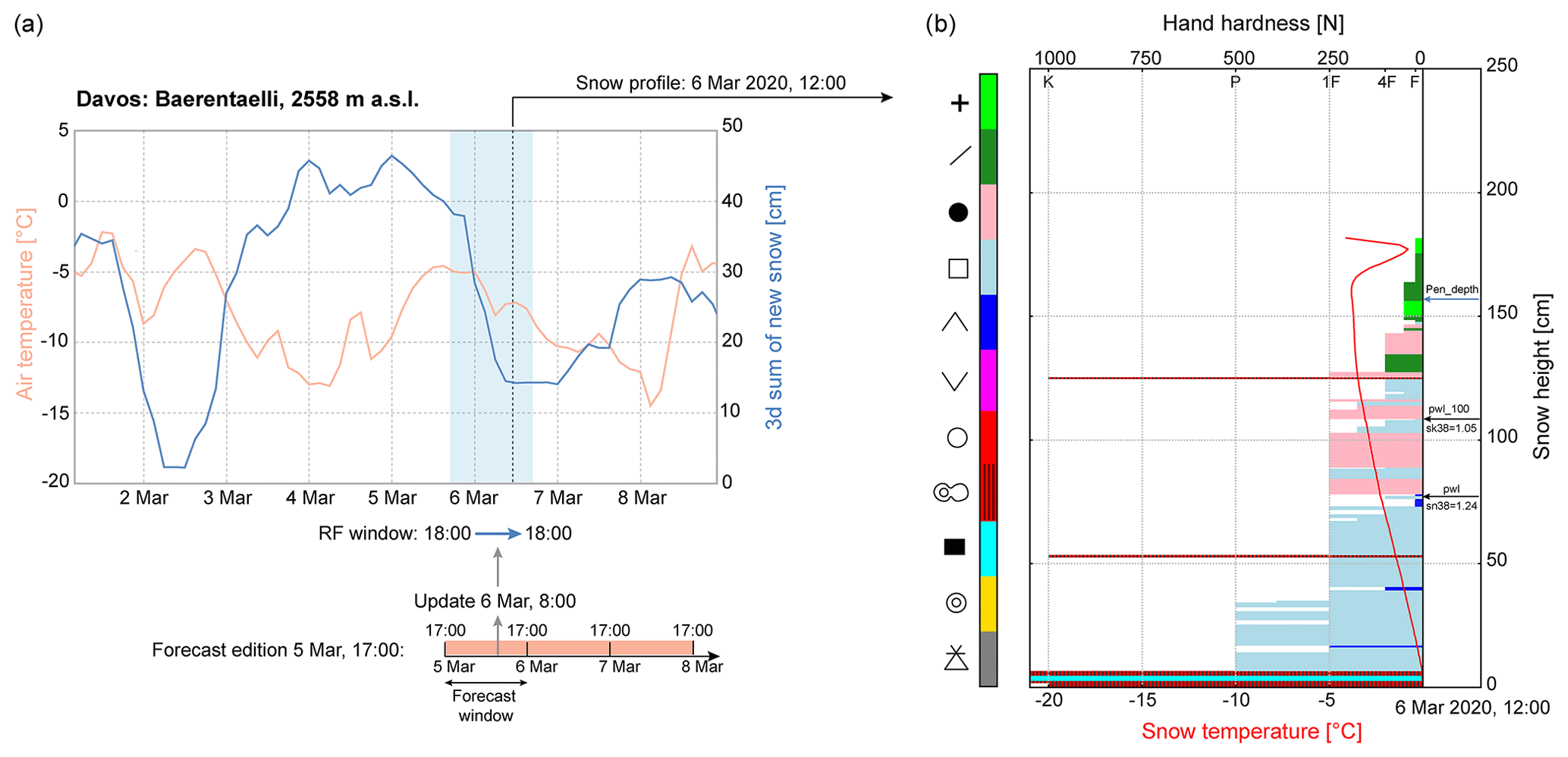
Figure 4(a) A 7 d time series (March 2020) of two meteorological features: air temperature (measured) and 3 d sum of new snow height (simulated by SNOWPACK) at the IMIS snow station Baerentaelli, which is located near Davos at 2558 m a.s.l. The blue area delimits an example of a 24 h time window (random forest, RF, window) from 5 March 2020 at 18:00 LT to 6 March 2020 at 18:00 LT, which is used to extract the averaged values used as inputs for the random forest algorithm. The avalanche forecast updated on 6 March 2020 at 08:00 LT is used for labelling the danger rating over the entire RF window. (b) Simulated snow stratigraphy from SNOWPACK at the same station on 6 March 2020 at 12:00 LT showing hand hardness, snow temperature, and grain type (colours). Hand hardness index F corresponds to fist, 4F to four fingers, 1F to one finger, P to pencil, and K to knife. Labels of grain types and colours are coded following the international snow classification (Fierz et al., 2009). The black arrows indicate the two critical weak layers located in the first 100 cm of the snow surface (PWL_100) and in a deeper layer (PWL), which were detected with the threshold sum approach. The blue arrow indicates the skier penetration depth (Pen_depth).
3.2.1 Meteorological input features
The meteorological time series with a 3 h resolution are resampled to non-overlapping 24 h averages, for a time window from 18:00 LT of a given day to the following day at 18:00 LT (24 h window in Fig. 4a), which is the nearest to the publication time of the forecast (17:00 LT).
Besides the 24 h mean, we also trained models considering as input values the standard deviation, maximum, minimum, range, and differences between subsequent 24 h windows during the exploratory phase. However, we noted that using these additional features did not improve the overall accuracy. In addition to the data describing the day of interest, we also extracted values for the last 3 and 7 d (Table C1). If there were missing values in the pre-processed time series, we removed these samples.
3.2.2 Profile input features
The simulated snow profiles provide highly detailed information on snow stratigraphy as each layer is described by many parameters and each profile may consist of dozens of layers. To reduce the complexity of the snow profile output and to obtain potentially relevant features, we extracted parameters defined and used in previous studies from the profiles at 12:00 LT, which we consider the time representative of the forecast window (Fig. 4b, Table C2). These parameters included the skier penetration depth (Pen_depth; Jamieson and Johnston, 1998) and snow instability variables such as the critical cut length (ccl; Gaume et al., 2017; Richter et al., 2019), the natural stability index (Sn38; Föhn, 1987; Jamieson and Johnston, 1998; Monti et al., 2016), the skier stability index (Sk38; Föhn, 1987; Jamieson and Johnston, 1998; Monti et al., 2016), and the structural stability index (SSI; Schweizer et al., 2006). We extracted the minimum of the critical cut length considering all layers below the penetration depth (min_ccl_pen). We retrieved the instability metrics for two depths where potentially relevant persistent weak layers existed following the threshold sum approach adapted for SNOWPACK (Schweizer and Jamieson, 2007; Monti et al., 2014). We located the persistent weak layer closest to the snow surface but within the uppermost 100 cm of the snowpack (PWL_100 in Fig. 4b) and then searched for the next one below (PWL in Fig. 4b). For these two layers, we extracted the parameters related to instability (ccl, Sn38, Sk38, SSI). If no persistent weak layers were found following this approach and to avoid missing values in the data, we assigned the respective maximum value of ccl, Sn38, Sk38, and the SSI observed within the entire data set, indicating the absence of a weak layer.
3.3 Assigning labels to extracted features
We assigned a class label (danger level) to the extracted features by linking the data of the respective station with the forecast for this warning region and RF window (Figs. 2b and 3b). Thus, each set of features extracted for an individual IMIS station (Fig. 1) was labelled with the forecast danger level for the day of interest.
Since avalanche danger depends on slope aspect and elevation, the public forecast describes the slope aspects and elevations where the danger level applies (Fig. 2). Outside the indicated elevation band and aspects, the danger is lower, typically by one danger level (SLF, 2020). Therefore, we discarded the data from stations on days when the elevation indicated in the forecast was above the elevation of the station. If no elevation was indicated, which is normally the case at 1-Low, we included all stations. We did not filter the data for the forecast slope aspects since the modelled features were obtained with flat-field SNOWPACK simulations.
To further enhance the data quality, we removed data of unlikely avalanche situations. Those included data when the danger level was for 4-High but the 3 d sum of new snow (HN72_24, Table C1) was less than 30 cm or when the snow depth was less than 30 cm.
3.4 Splitting the data set
We split our data set into training and test sets corresponding to different winter seasons to ensure that training and test data were temporally uncorrelated. We defined the test set as the two most recent winter seasons of 2018/19 and 2019/20 (Fig. 3d). The training set corresponded to the remaining data, including the seasons from 1997/98 to 2017/18 (21 winters). The size of the test set is 10 % of the total number of data and will be used for a final, unbiased evaluation of the model's generalization.
We optimized the model's hyperparameters and selected the best subset of features using 5-fold cross-validation on the training set, which is an effective method to reduce overfitting. Each subset contains data of three to five consecutive winter seasons with an approximate size of 20 % of the training data set (N=230 550 in Fig. 3c): 1997/98 to 2002/03 (Fold 1, 19 % of samples), 2003/04 to 2006/07 (Fold 2, 18 % of samples), 2007/08 to 2009/10 (Fold 3, 19 % of samples), 2010/11 to 2013/14 (Fold 4, 22 % of samples), and 2014/15 to 2017/18 (Fold 5, 22 % of samples). This partitioning again ensures that feature selection was not affected by temporally correlated data. Models were trained and tested five times, using as a validation test set each of the defined folds and as a training set the remaining data. The final score was averaged over the five trials.
We approach the nowcast assessment of the avalanche danger level as a supervised classification task that involves assigning a class label corresponding to the avalanche danger level to each set of meteorological and simulated snow cover data from an automatic weather station network located in Switzerland.
We tested a variety of widely used supervised learning algorithms, and the best scores were obtained with random forests (Breiman, 2001), which are among the most state-of-the-art techniques for classification. Random forests are powerful nonlinear classifiers combining an ensemble of weaker classifiers, in the form of decision trees. Each tree is grown on a different bootstrap sample containing randomly drawn instances with replacement from the training data. Besides bagging, random forests also employ random feature selection at each node of the decision tree. Each tree predicts a class membership, which can be transformed into a probability-like score by computing the frequency at which a given test data point is classified across all the trees. The final prediction is obtained by taking a majority vote of the predictions from all the trees in the forest or, equivalently, by taking the class maximizing the probability.
Our classification problem is extremely imbalanced; danger level 4-High (Fig. 3) accounts for only a small fraction of the whole data set. Imbalanced classification poses a challenge for predictive modelling as most existing classification algorithms such as random forests were designed assuming a uniform class distribution of the training set, giving rise to lower accuracy for minority classes (Chen et al., 2004). Since danger level 5-Very High is very rarely forecast (<0.1 %), we merged it with 4-High. This step reduced the multi-class classification problem to four classes. We also explored diverse data sampling techniques (results not shown), such as down-sampling the majority classes or over-sampling the minority classes, to balance the training data when fitting the random forest. However, since none of these methods showed an improvement in the performance and given the imbalanced nature of the data, we discarded these strategies. Hence, we opted for learning from our extremely imbalanced data set applying cost-sensitive learning. With this approach, we employed a weighted impurity score to split the nodes of the trees, where the weight corresponds to the inverse of the class frequency. This ensures that prevalent classes do not dominate each split and rare classes also count towards the impurity score. We used the standard random forest implementation from the scikit-learn library (Pedregosa et al., 2011).
We trained two random forest models: RF 1 was trained using the labels from the complete data set of forecast danger levels (Dforecast, Fig. 3b), while RF 2 was trained with the much smaller data set of tidy danger levels (Dtidy, Fig. 3b). We compared their performance on a common test set. Both models were trained by pooling the data from all IMIS stations.
4.1 Model selection
We selected the best random forest model by a three-step cross-validation strategy. For this, we used cross-validation maximizing the macro-F1 score, which corresponds to the unweighted mean of F1 scores computed for each class (danger level), independently. The F1 score is a popular metric for classification, as it balances precision and recall into their harmonic mean, ranging from 0 (worst) to 1 (best). The macro-F1 score showed the best performance for both minority and majority classes. All the metrics used to evaluate the performance of the models are defined in Appendix B.
In the first step, we selected a set of hyperparameters from a randomized search, which maximizes the macro-F1 score. After choosing the first optimum set of hyperparameters, we selected the 30 best input features by ranking them according to the feature importance score given by the random forest algorithm, which is the average impurity decrease computed from all decision trees in the forest. In the third step, we refined the hyperparameters by a dense grid search centred around the best parameters from the first step but using the optimum feature set. This strategy shows optimal accuracy for all the classes while keeping the model as small as possible in terms of features. For the previous steps, a 5-fold cross-validation approach was applied. For each set of hyperparameters, in the random grid search and the grid search, each model was trained and tested five times such that each time, one of the defined folds (Sect. 3.4) was used as a test set and the other four folds were part of the training set. The macro-F1 estimate was averaged over these five trials for each hyperparameter vector. The final hyperparameters selected are shown in Table B1.
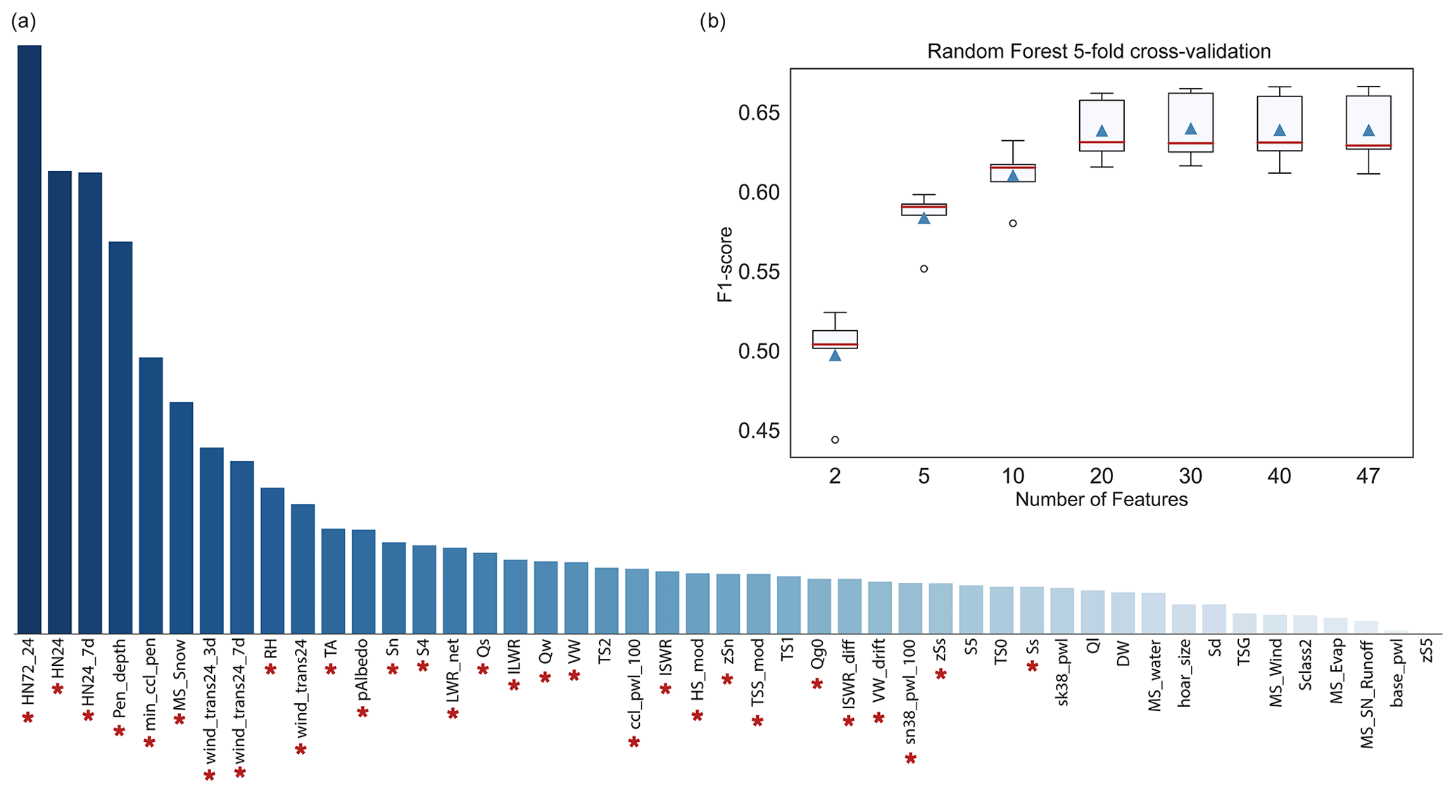
Figure 5(a) Feature importance ranking scored by random forest classifier (y axis normalized). A description of each feature is provided in Tables C1 and C2 of Appendix C. The red asterisks denote the final set of features selected to train the models. (b) Box plot of the distribution of the macro-F1 score (5-fold cross-validation) for the random forest classifier with a varying number of features from 2 to 47.
4.2 Feature selection
We used different approaches to remove unnecessary features and select a subset that provides high model accuracy while reducing the complexity of the model. First, variables that are strongly correlated were dropped (). For a given pair of highly correlated weather features, we removed the one showing a lower random forest feature importance score (obtained from the first step described above), which is shown in Fig. 5a. Feature importance is the average impurity decrease computed from all decision trees in the forest. In the case of correlation between profile features, we kept the variables extracted from the uppermost weak layer that is usually more prone to triggering. A total of 20 highly correlated variables were removed from the initial data set, leaving 47 features (Tables C1 and C2). The overall performance of the model remained the same after removing these features. In addition, we manually discarded the snow temperatures (TS0, TS1, and TS2) measured at 25, 50, and 100 cm above ground (Fig. 5a and Table C1) as their incorporation into the model requires a larger minimum snow depth (>100 cm) for meaningful measurements.
Figure 5a shows that the features with the highest importance were various sums of new snow and drifted snow, the snowfall rate, the skier penetration depth, the minimum critical cut length in a layer below the penetration depth, the relative humidity, the air temperature, and two stability indices. Hence, the highest-ranked features selected by the random forest classifier were in line with key contributing factors used for avalanche danger assessment (Perla, 1970; Schweizer et al., 2003).
To select the best subset of features, we applied the approach of recursive feature elimination (RFE) (Guyon et al., 2002), which is an efficient method to select features by recursively considering smaller sets of them. An important hyperparameter for the RFE algorithm is the number of features to select. To explore this number, we wrapped a random forest classifier, which was trained with a variable number of features. Features were added in descending order from the most to the least important in the score ranking estimated by the random forest (Fig. 5a). Figure 5b shows the variation in the mean of the macro-F1 score with the number of selected features. The performance improves as the number of features increases until the curve levels off for 20 or more features. We selected a subset of 30 features (highest macro-F1 score). The final set of features selected applying RFE are highlighted with red asterisks in Fig. 5a and are were used to train the two final models RF 1 and RF 2 (complete and tidy data sets). Note that the application of RFE, although it might seem redundant with the internal feature ranking made by the random forest algorithm, ensures that the growing subset of features provides consistent improvements and the feature selection is not biased by the way the impurity score is computed (Strobl et al., 2007).
In the following, we first present key characteristics describing the overall performance of the RF classifiers (Sect. 5.1). To explore the temporal variation in their performance, we analyse the average prediction accuracy on a daily basis considering the uncertainty related to the forecast danger level (Sect. 5.2). In Sect. 5.3 and 5.4, we investigate the spatial performance of the models in different climate regions and for different elevations. Finally, we assess the performance for cases when the danger level changes or stays the same (Sect. 5.5) and for the case when the danger level of the previous day is added as an additional input feature (Sect. 5.6).
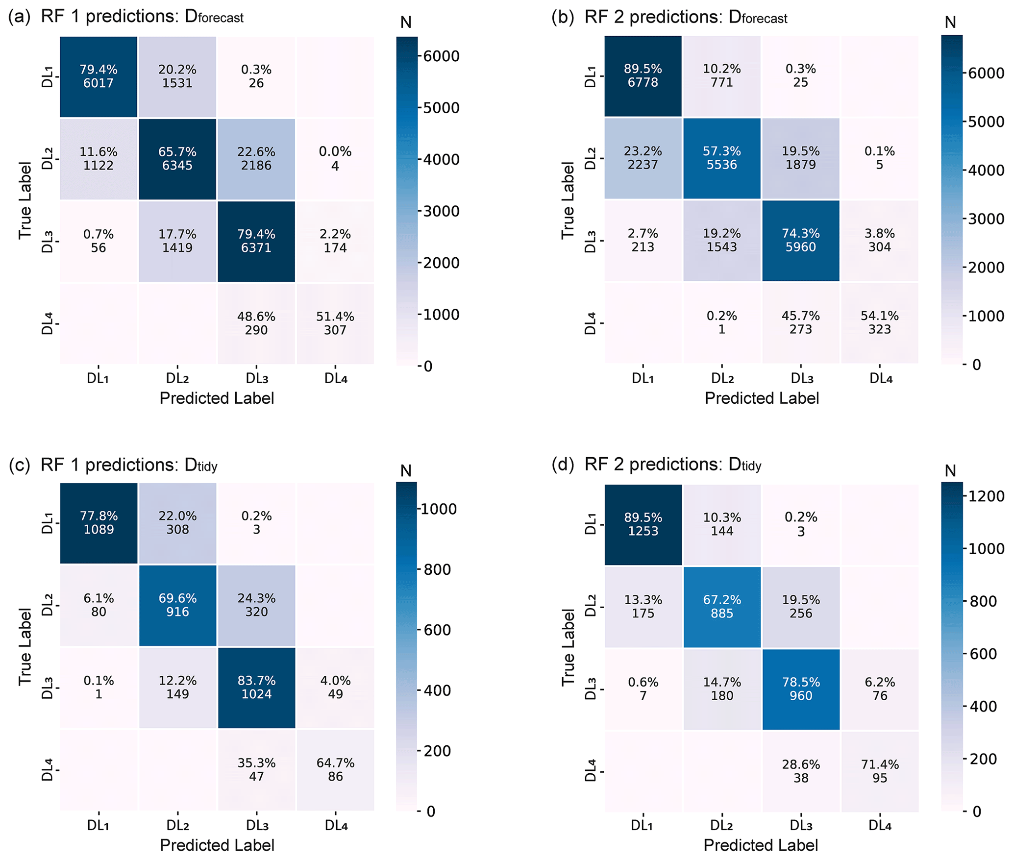
Figure 6Confusion matrices of the two random forest models, RF 1 (trained with Dforecast) and RF 2 (trained with Dtidy), applied to the test set data of (a) the forecasted danger levels and (b) the tidy danger levels of the winter seasons of 2018/19 and 2019/20.
5.1 Performance of random forest classifiers
We trained two models, RF 1 and RF 2, and tested them against two different data sets, which contain the winter seasons of 2018/19 and 2019/20 (Fig. 3d). When evaluating the performance of the models against the test set Dforecast, RF 1 achieved an overall accuracy (number of correctly classified samples over the total number of samples) of 0.74 and a macro-F1 score of 0.7 (Table 1a). Even though RF 2 was trained with only 9 % of the data (Fig. 3c), it reached an almost similar overall accuracy of 0.72 and a macro-F1 score of 0.68 (Table 1b). F1 scores for each class were also fairly equal for both models (Table 1a and b). However, for the minority classes of danger levels 1-Low and 4-High, the precision of RF 1 was higher, whereas a higher proportion of samples were correctly classified by RF 2 (higher recall). This result highlights the impact of using better-balanced training data in RF 2 and less noisy labels.
Table 1Test set model performance scores of the two final random forest models (RF 1 and RF 2): precision (Prec.), recall (Rec.) and F1 for each danger level (DL; 2-Moderate and 3-Considerable are denoted as 2-Mod. and 3-Cons., respectively), overall accuracy (Acc.) and macro-F1 score. (a) Predictions RF 1 vs. Dforecast (ground truth). (b) Predictions RF 2 vs. Dforecast (ground truth). (c) Predictions RF 1 vs. Dtidy (ground truth). (d) Predictions RF 2 vs. Dtidy (ground truth).
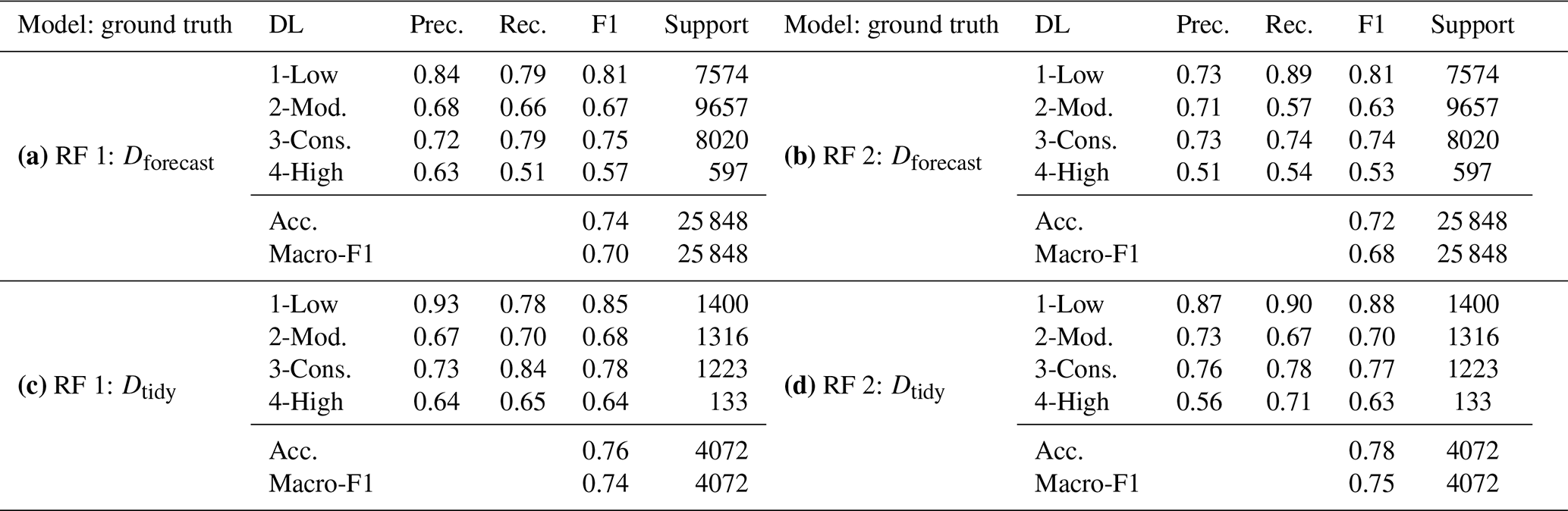
The performance of the models tested on Dtidy showed that RF 2 achieved the highest macro-F1 score of 0.75 and overall accuracy of 0.78 (Table 1d), with very similar values for RF 1 (accuracy 0.76, macro-F1 score 0.74). The class breakdown for the two models showed better scores when tested against Dtidy compared to Dforecast. The performance increased most notably for danger level 4-High, with the F1 score reaching 0.64.
The confusion matrices shown in Fig. 6 provide more insight into the performance of both models. The values on the diagonal clearly dominate. This indicates that the majority of cases was correctly predicted by the classifiers, as is also shown in Table 1 (the percentages shown in the diagonal correspond to the recall in Table 1). Furthermore, if predictions deviated from the ground truth label, the difference was in most cases one danger level and only rarely two danger levels (<3 %).
To analyse the model bias in more detail, we defined a model bias difference ΔDL as
where DLRF is the danger level predicted by the random forest model and DLTrue is the ground truth danger level. Table 2 summarizes the percentages of test samples for each model bias difference.
Table 2Model (M) used for training and ground truth (GT) labels of the test set, bias (ΔDL), and the proportion of samples (P) for each bias value. Both models are evaluated on the Dforecast test set (upper part) and Dtidy test set (lower part).
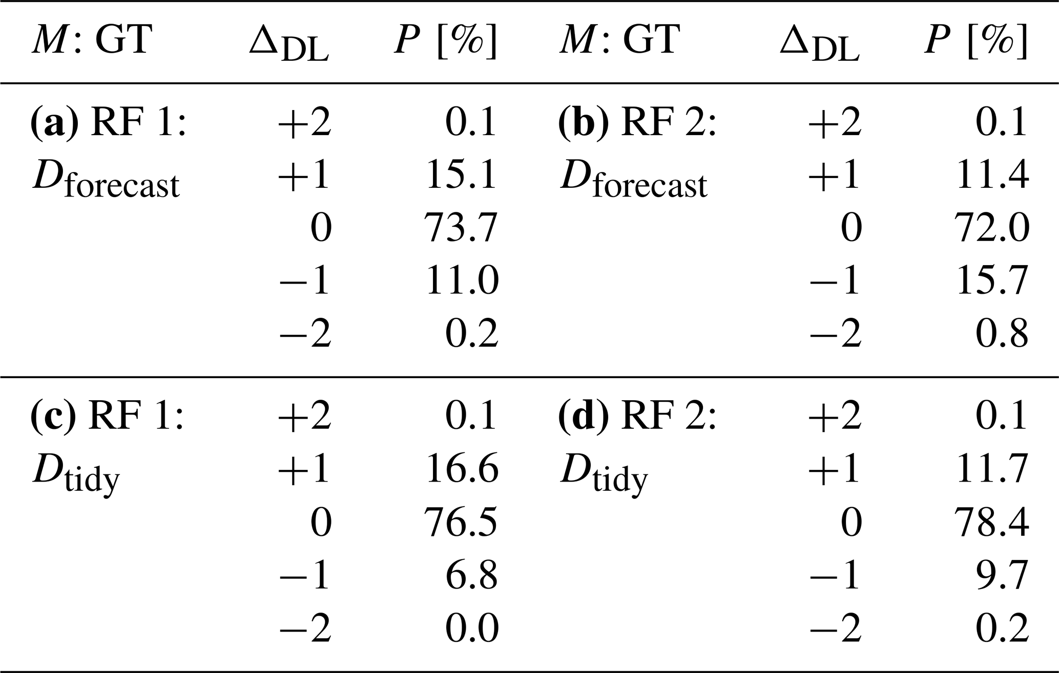
Compared to Dforecast, RF 1 exhibited a bias towards higher danger levels (∼15 %) rather than lower ones (∼11 %; Table 2a), while RF 2 showed an inverse trend of deviations (Table 2b). Compared with Dtidy, RF 1 showed an even larger bias towards higher danger levels (Table 2b), compared to RF 2, which had an almost equal proportion of predictions which were higher (12 %) or lower (10 %). Regardless of which of the two models was evaluated, predictions tended to be higher for 2-Moderate (ΔDL=1; between 20 % and 24 % in Fig. 6) and lower for 3-Considerable (; between 12 % and 19 % in Fig. 6). As 1-Low and 4-High are at the lower and upper end of the scale, respectively, wrong predictions can only be too high at 1-Low and too low at 4-High.
In summary and as can be expected, each model performed better when compared to its respective test set. RF 1 achieved better performance compared to RF 2 when evaluating them on the Dforecast test set, while RF 2 achieved slightly higher performance on the Dtidy test set. The performance of RF 1 improved when tested against the best possible test data (Dtidy), particularly for the danger level 4-High.
5.2 Daily variations in model performance and the impact of the ground truth quality on performance values
In the next step, we compare the predictive performance of the two random forest models during the two test seasons by analysing the performance on a daily basis. To this end, we only consider the predictions using the forecast danger level (Dforecast) as the number of predictions per day is much larger than in the tidy data set. Nevertheless, when discussing the performance of the models, we must also consider the uncertainty related to this target variable as errors in the ground truth can significantly impact the performance of the models. This is particularly important in our case as we rely on the forecast danger level (Dforecast) as the ground truth label. To conduct this evaluation, we compare the daily accuracy of the models with the “accuracy” of the forecast, which we estimate by comparing the regional forecast to the local nowcast provided by experienced observers. The comparison of the forecast with the local nowcasts provides the most meaningful reference point for the evaluation of the models.
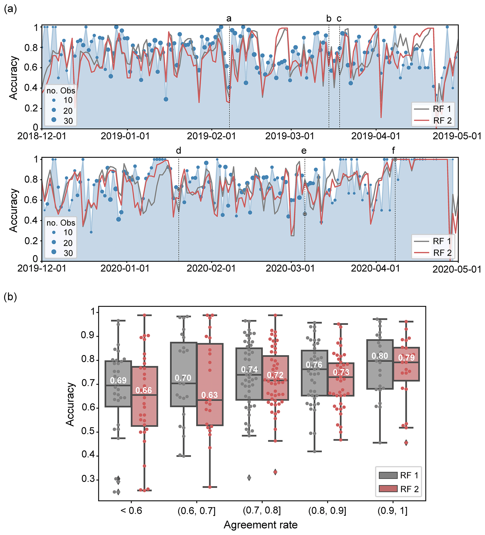
Figure 7(a) Comparison of the time series of the daily accuracy of the two random forest models, RF 1 (trained with Dforecast) and RF 2 (trained with Dtidy), tested on the winter seasons of 2018/19 (top) and 2019/20 (bottom) for predicting the danger level forecasts. The blue-shaded area represents the agreement rate, and the points show the number of observers that provided an assessment. The dashed lines show the six dates (labelled from a to f) selected as exemplary cases (see Appendix D). The date is indicated in the format year-month-day. (b) Box plots of the distribution of the accuracy of the models, grouped together by the agreement rate. Dots are the individual data points.
To estimate the accuracy of the forecast, we rely on the local nowcast reported by observers (Sect. 2.3). Thus, we consider the agreement rate between the forecast danger level (DLF) and nowcast danger level (DLN) as a proxy for the accuracy of the forecast (e.g. Jamieson et al., 2008; Techel and Schweizer, 2017). The agreement rate (Pagree) for a given day is then the normalized ratio of the number of cases where nowcast and forecast agree () to the number of all forecast–nowcast pairs (N):
On average, regional forecasts and local nowcasts agreed 75 % of the time (N=5099). However, considerable variations in the daily agreement rate can be noted in Fig. 7a, where the agreement rate is represented by the blue-shaded area and where the points show the number of observers that provided an assessment. Considering the 171 dates with more than 15 assessments, the agreement rate ranged between 27 % and 100 % (median 77 %, interquartile range 65 %–85 %), suggesting that the accuracy of the forecast is lower than the overall model accuracy on about half of the days.
The daily accuracy of the predictions of the two models, the overall match between the model outputs and Dforecast as ground truth, is shown in Fig. 7a. Variations in the daily accuracy of the two models were highly correlated (Pearson correlation coefficient 0.88). The average difference in the daily accuracy between the two RF models is 0.07; on 75 % of the days it was less than 0.1. Overall, the performance of RF 1 was slightly better than RF 2 as is reflected in the overall scores (Table 1a and b) and as can be expected when comparing with Dforecast because RF 1 was trained with this data set. The match between predictions and Dforecast is comparably high on about half of the days (RF 1 accuracy > 0.74, RF 2 accuracy > 0.70) and less than 0.5 on 11 % (RF 1) and 15 % (RF 2) of the days.
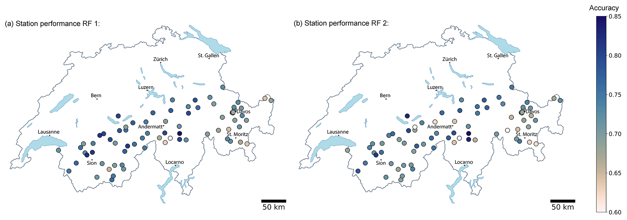
Figure 8Maps showing the average accuracy of (a) RF 1 and (b) RF 2 model predictions for the 73 IMIS stations for which predictions were available on at least 50 % of the test set (Dforecast) days.
Figure 7b summarizes the correlation between the daily prediction accuracy of the two RF models, evaluated against Dforecast, and the agreement rate between forecast and nowcast assessments. Again, we consider only days when at least 15 observers provided a nowcast assessment. Overall, the performance of both models decreased with a decreasing agreement rate. When the agreement was high (Pagree>0.9, Fig. 7b) and hence the forecast in many places likely correct, the performance of RF 1 was particularly good (median accuracy of 0.8), whereas the accuracy of RF 2 was slightly lower (median accuracy of 0.79). When the agreement rate was low (Pagree<0.6, Fig. 7b) and hence the forecast at least in some regions likely wrong, the predictive performance of model RF 2, trained with the tidy danger level labels, is considerably lower, resulting in a median accuracy of 0.66. In contrast, RF 1, which was trained with the over-forecast bias present in the Dforecast data, was less impacted (median ∼ 0.7).
To further illustrate the daily performance of the models, we created two videos (Supplement) with the maps showing the predictions of each model at each IMIS station together with the local nowcast assessments and the forecast danger level. In addition, we also describe the predictions on six selected dates that differed in terms of forecast agreement rate and model performance (see Appendix D).
5.3 Station-specific model performance
Our objective was to develop a generally applicable classifier for predicting the danger level at all IMIS stations in the Swiss Alps. In other words, the classifier should show a similar performance independent of the location of the station. To explore this, we analysed the station-specific averaged accuracy for the entire test set (Dforecast) of both models for the 73 stations for which predictions were available on at least 50 % of the days.
The maps displayed in Fig. 8 show that the station-specific accuracies ranged between 0.6 and 0.85 (mean accuracy of 0.73) for RF 1 and between 0.5 and 0.87 (mean accuracy of 0.72) for RF 2. Some spatial patterns in the performance of both models are visible (Fig. 8), indicating that differences between stations are not random: both models performed consistently well in the northern and western parts of the Swiss Alps with the accuracy being above the mean for many stations, compared to lower accuracy in the eastern part of the Alps (accuracy < 0.7). RF 1 performed somewhat better in the southern and central parts of Switzerland and RF 2 in the northern parts. At stations with lower performance (accuracy < 0.7), we observed that the danger levels 1-Low or 3-Considerable were less frequently forecast in these regions (proportion of days ∼3 % lower) than in the rest of Switzerland. As the prediction performance was higher at these danger levels (Table 1a and b), this may partly explain the geographical differences in performance.
5.4 Model performance with elevation
Here we address the impact of filtering for elevation, which we applied for data preparation when defining the training and test data. We trained the classifiers exclusively with data from stations which were above the elevation indicated in the bulletin (Sect. 3.3; see also Fig. 2). To explore whether this decision was appropriate, we now compare the prediction accuracy of RF 1 as a function of the difference in elevation between the stations and the elevation indicated in the bulletin: .
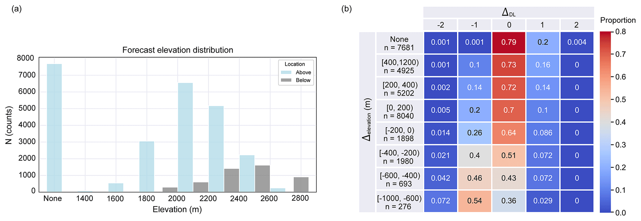
Figure 9(a) Frequency of the elevation indicated in the public forecasts with the number of stations that are located above and below this elevation. The class of none contains the samples for the days when no information was indicated in the bulletin. (b) Heat map of the proportions of samples (row-wise normalized) for each of the eight elevation classes () versus the range of prediction bias (ΔDL) of the model RF 1. The total number of samples in each elevation class is denoted with n.
In the public bulletin, the elevation information is given in incremental intervals of 200 m in the range between 1400 and 2800 m a.s.l. for dry-snow conditions. To obtain more insight into the performance of the model in relation to the elevation, we separated the predictions into those for stations located above (N=25 848) and below (N=4847) the elevation indicated in the bulletin (Fig. 9a). Generally, on any given day, the elevation indicated in the forecast is lower than the elevation of most stations.
Table 3Accuracy of RF predictions (proportion of samples – row-wise sum for “Overall” and column-wise sum for the rest) of a RF classifier tested against Dforecast as a function of changes in the forecast danger level compared to the day before, for cases when the danger level increased (↗), stayed the same (→), or decreased (↘) for (a) RF 1 and (b) RF 1*, a model which additionally considers the forecast danger level of the previous day as an input feature.

To analyse the model performance in more detail, we defined eight classes of Δelevation. Figure 9b shows the eight classes and their definitions, each containing the proportion of samples (row-wise sum) as a function of the model bias difference defined in Eq. (1). The class “none” contains the samples for the days when no elevation information was provided in the bulletin. This class essentially corresponds to forecasts with danger level 1-Low (99 %). This is the most accurate class, reaching an accuracy at ΔDL=0 of 79 %, which is the same as the recall for 1-Low shown in Table 1a. Overall, the prediction accuracy was highest for stations with an elevation far above the elevation indicated in the forecast (accuracy 0.73 for Δelevation≥400 m) and lowest for stations located far below this elevation (accuracy 0.36 for m, Fig. 9b). At the same time, the bias in the predictions, compared to Dforecast, changed from being slightly positive (ratio of the proportion of predictions higher to those lower than forecast is 1.6 for Δelevation≥400 m) to negative (Δelevation≤200 m) and to primarily being negative for stations far below this elevation (ratio of predictions lower to those higher than forecast is 18 for m, Fig. 9b).
5.5 Model performance with respect to increasing or decreasing hazard
When evaluating the agreement rate of the avalanche forecast with the local nowcasts, Techel and Schweizer (2017) distinguished between days when the avalanche danger increased and days when it decreased. When the danger increases, changing weather primarily drives the decrease in snow stability. In contrast, decreasing avalanche danger is often linked to comparably minor and/or slow changes in snowpack stability (e.g. Techel et al., 2020b). While these changes are gradual in nature, these can only be expressed in a step-like fashion using the five-level danger scale. For the purpose of this analysis, we followed the approach by Techel and Schweizer (2017) and split the data set into days when the danger level increased, stayed the same, or decreased, in relation to the previous day.
As shown in Table 3a, the accuracy was highest on days when the forecast danger level stayed the same (0.77), compared to days when the forecast danger increased (accuracy 0.67; support 10 %) or decreased (accuracy 0.59; support 14 %). Considering that Techel and Schweizer (2017) reported the lowest agreement between forecast and nowcast for days when the forecast increased suggests that we evaluate these cases with danger level labels which were proportionally more often wrong.
5.6 Model performance considering the forecast danger level from the previous day
The avalanche warning service reviews daily the past forecast in the process of preparing the future forecast (Techel and Schweizer, 2017). Hence, the past forecast can be seen as the starting point for the future forecast. Therefore, we also tested whether the prediction performance changed when including the forecast danger level from the previous day's forecast as an additional feature in the random forest model (RF 1*). As shown in Table 3b, not only did the overall accuracy increase notably from 0.74 (RF 1) to 0.82 (RF 1*) but also accuracy increased for all the danger levels individually. However, when additionally considering the change to the previous day's forecast, this comes at the cost of a large decrease in the performance in situations when the danger level changed (DL increased for 10 % and decreased for 14 % of the total samples). For these situations, there is a drop in accuracy, overall from 0.67 (RF 1) to 0.43 (RF 1*) when the danger level increased and from 0.59 (RF 1) to 0.29 (RF 1*) when the danger level decreased.
We first discuss the following key characteristics of the training data (Sect. 6.1), which may impact both the construction of the RF classifiers and their performance evaluation:
-
the size of the data set in relation to the complexity of the addressed classification problem;
-
the class distribution, with particular attention to minority classes; and
-
the quality of the labels, i.e. the accuracy of the regional forecasts by human experts.
We also address scale issues – a danger level describing regional avalanche conditions for a whole day compared to measurements and SNOWPACK simulation output describing a specific point in time and space (Sect. 6.2). In Sect. 6.3, we discuss the performance of the RF classifiers considering one of our key objectives, namely to develop a model applicable to the entire forecast domain of the Swiss Alps, before we compare the developed RF classifiers with previously developed models predicting a regional avalanche danger level (Sect. 6.4). Finally, we provide an outlook on the operational pre-testing of the models (Sect. 6.5) and their future application for avalanche forecasting (Sect. 6.6).
6.1 Impact of training data and forecast errors on model performance
6.1.1 Training data volume and class distribution
In general, a large training data set increases the performance of a machine learning model as it provides more coverage of the data domain. However, Rodriguez-Galiano et al. (2012) showed that random forest classifiers have relatively low sensitivity to the reduction in the size of the training data set. In fact, the large reduction in the number of training data of RF 2, containing only 10 % of data of RF 1, did not have a substantial impact on model performance. RF 2 had similar overall scores when evaluated on the Dforecast test set (Table 1a and b) and even slightly higher scores on the Dtidy test set (Table 1c and d) as it was trained with Dtidy. The dominant classes of danger levels, 2-Moderate and 3-Considerable, were the most affected ones, showing a decrease in accuracy of between 5 % and 8 % (Fig. 6a and b).
Furthermore, RF 2 is trained using a better-balanced training data set (Fig. 3c). The confusion matrices exhibit an improvement of the per class accuracy (Fig. 6), i.e. the recall percentages of the diagonal matrix, of the minority classes of danger levels 1-Low and 4-High when using RF 2, reflecting the positive impact of balancing the training ratio for these danger levels.
6.1.2 Quality of avalanche forecasts
Even though previous applications of random forests have demonstrated that they comprise one of the most robust classification methods tolerating some degree of label noise (e.g. Pelletier et al., 2017; Frénay and Verleysen, 2013), their performance decreases with a large number of label errors (Maas et al., 2016). Labelling errors, however, may influence the model building, which can be particularly relevant for minority classes such as danger level 4-High. Furthermore, such errors in the ground truth may also lead to seemingly lower prediction performance (e.g. Bowler, 2006; Techel, 2020). Aiming to reduce the impact of wrong class labels, we compiled the best possible, presumably more accurate, ground truth data set (Dtidy), which was used to train RF 2.
To assess the accuracy of the forecast and thus potential errors in the forecast danger levels (Dforecast), we relied on nowcast assessments (DLN) by well-trained observers. Although the local nowcasts are also subjective assessments, they are considered the most reliable data source of danger levels (Schweizer et al., 2021; Techel and Schweizer, 2017). Previous studies estimated the accuracy of the Swiss avalanche forecasts to be in the range between 75 % and 81 % (this study – see Sect. 5.2; Techel and Schweizer, 2017; Techel et al., 2020b). Our classifiers reached these values: the overall prediction accuracies of RF 1 and RF 2 were 74 % and 72 % (compared to Dforecast) and 76 % and 78 % (compared to Dtidy), respectively (Table 1). Particularly, the accuracy of the minority class 4-High improved for RF 2 (Fig. 6), emphasizing the importance of training and testing against the best possible data set Dtidy. To compile this data set, quality checking was particularly important for danger level 4-High (Sect. 3.1.2 and Appendix A) since the forecast is known to be comparably often erroneous when this danger level is forecast (e.g. Techel and Schweizer, 2017; Techel, 2020). In the future, a new compilation of Dtidy resulting in a larger data volume may improve the predictive performance.
Considering the predictions on particular days (Fig. D1), some stations predicted the danger level, which was forecast in the adjacent warning region. This suggests that occasionally the boundary between areas of different forecast danger levels could be questionable. Such errors in the spatial delineation of the extent of regions with the same danger level have also been noted by Techel and Schweizer (2017). They showed that the agreement rate between the local nowcast assessments and the regional forecast danger level was comparably low in warning regions which were neighbours to warning regions with a different forecast danger level. Hence, incorrect boundaries may have further contributed to label noise.
Similarly, errors in the elevation indicated in the bulletin may have an impact as we used this forecast elevation to filter data (Sect. 3.3). The effect of the forecast elevation on the classifier performance was clearly visible with the accuracy decreasing for stations below the elevation indicated in the bulletin, often showing a bias of −1 danger level (Fig. 9). This result agrees with the assumption that the danger is lower below the elevation indicated, typically by one danger level (Winkler et al., 2021). However, the proportion of correct predictions at stations close to but below the elevation indicated was fairly high (0.64), which may reflect a more gradual decrease in the danger level with elevation (Schweizer et al., 2003). This finding suggests that the model is able to capture elevational gradients of avalanche danger.
6.2 Spatio-temporal scale issues
The temporal and spatial scale of the avalanche forecast and data used to train the model should be considered when verifying a forecasting model (McClung, 2000). To match the temporal scale, we extracted the meteorological and snowpack features for the time window closest to the avalanche forecast. Nevertheless, for avalanche forecasting, “forecast” data from weather predictions strongly drive the decision-making process. The RF models, however, were trained using “nowcast” data (recorded measurements and simulated data based on these measurements). This may introduce an additional bias between the danger level predictions of the model and the public forecast. The use of the morning forecast, whenever it was available as ground truth, reduced this bias. Nevertheless, a model trained with forecast input data may improve the performance.
A scale mismatch exists between our target variable and the model predictions. Whereas the same danger level is usually issued for a cluster of warning regions, characterized by a mean size of 7000 km2 (Techel and Schweizer, 2017), the predictions of the model reflect the local conditions measured and modelled at an individual IMIS station. Hence, the spatial scale difference can be of more than 2 orders of magnitude. Stations located in the same or nearby warning regions forecast with the same danger level sometimes predict different danger levels (Fig. D1) as avalanche conditions may vary even at the scale of a warning region (Schweizer et al., 2003). These local variations are inherent to the characteristics of the station such as elevation, wind exposure, and more. To overcome the spatial scale issues in future applications, predictions could be clustered through ensemble forecasting methods.
6.3 Spatio-temporal variations of the model performance
Snow stability and hence avalanche danger evolve in time – driven primarily by changing weather conditions – and vary in space – depending on the terrain and how meteorological conditions affect the snowpack at specific locations.
Overall, the two models captured this evolution with an overall accuracy of more than 72 % (Table 1) or 67 % (RF 1) when considering only times when the avalanche hazard increased (Table 3a). However, the accuracy of the models varied during the winter season (Fig. 7a), with about 10 %–15 % of the days exhibiting an accuracy < 0.5 (Sect. 5.1). Here, we distinguished two cases (Sect. 5.2): first, some days with such seemingly poor performance could be linked to the forecast danger level, the target variable used for validation, which was likely wrong in many areas. These cases were characterized by a low agreement rate, Pagree, between forecast and nowcast assessments, for instance on 7 February 2019 (Fig. D1a). However, not all the days with a poor model performance correlated with low values of Pagree (Fig. 7b). This suggests that variations in model performance may also be due to different avalanche situations and, hence, the ability of the classifiers to accurately predict them. Even though we have only qualitatively explored this, we observed that the predictive performance of both models sometimes decreased on days when the avalanche problem of “persistent weak layers” (EAWS, 2021a) was the primary problem.
Second, the performance of the models was lower at stations located in the eastern part of the Swiss Alps, for instance, in the regions surrounding Davos or St. Moritz (these are marked in Fig. 8). Since model accuracy varied in situations when the danger changed (Table 3), we verified whether the proportion of cases with a change in the danger level differed in these regions compared to other areas. However, changing danger levels were forecast about as often in these regions as in the rest of Switzerland, with, for instance, an increase in avalanche danger being forecast on 9 % to 10 % of the days in Davos and St. Moritz, compared to an overall mean of 10 % for the remainder of the Swiss Alps (decreasing danger level of 11 % to 12 % in St. Moritz and Davos, respectively, overall mean 14 %). The model performance was highest when danger level 1-Low was forecast (Table 1), which was somewhat less frequently the case in St. Moritz (24 %) and Davos (26 %) compared to the entire Swiss Alps (29 %, top of Fig. 3d). Furthermore, we also explored if the agreement rate between forecast and local assessments, an indicator for the quality of the danger level labels, was lower there. While Pagree was about 71 % for Davos, which was lower than the overall mean of 75 %, the agreement rate was 82 % for St. Moritz. Consequently, none of these effects may conclusively explain the variations observed. Again a possible explanation may be related to the snowpack structure in this part of the Swiss Alps, which is often dominated by the presence of persistent weak layers (e.g. Techel et al., 2015). However, this aspect of model performance must be analysed in more detail and goes beyond the scope of this work.
6.4 Comparison of data-driven approaches for danger level predictions
Some of the first attempts to automatically predict danger levels for dry-snow conditions were reported by Schweizer et al. (1994), who designed a hybrid expert system based on a training set of about 700 cases using a verified danger level, correctly classifying 73 % of the cases. Schweizer and Föhn (1996) also predicted the avalanche danger level for the region of Davos trained with the same data. The cross-validated accuracy was 63 %, showing an improvement to 73 % when adding further snowpack stability data and knowledge in the form of expert rules to the system.
Schirmer et al. (2009) compared several classical machine learning methods to predict the avalanche danger. They used as input measured meteorological and SNOWPACK variables from the AWS at Weissfluhjoch (WFJ2) station located above Davos. They reported an accuracy of typically around 55 % to 60 %, which improved to 73 % when the avalanche danger level of the previous day was an additional input. Although the test set used in this study is not directly comparable with the previous ones, the overall accuracies obtained with our classifiers are higher (Table 1). Still, the mean accuracy of the predictions at the stations located in the region of Davos was lower (Fig. 8), showing values of 72 % (RF 1 model) and 69 % (RF 2 model) for the station WFJ2. We also observed an important improvement in the overall performance of the model when adding the danger level of the previous day (Table 3b). However, the predictions were mainly driven by the danger level feature and RF 1* failed to predict the situations of increasing or decreasing avalanche hazard. This model would have limited usefulness in operational avalanche forecasting since it too strongly favours persistency in avalanche danger.
6.5 Operational testing of the models
During the winter season 2020/21, both RF models were tested in an operational setting providing a nowcast and a “24 h forecast” prediction in real time. The model chain consisted of the following steps, of which the first two steps are equivalent to the operational SNOWPACK model setup in the Swiss avalanche warning service (Sect. 2.1; Lehning et al., 1999; Morin et al., 2020): (1) measurements are transferred from the AWS to a server at SLF once an hour; (2) based on these data, snow cover simulations are performed with the SNOWPACK model for the location of the IMIS station and for four virtual slope aspects (“north”, “east”, “south”, and “west”) every 3 h; (3) the input features required for the RF models are extracted from the snow cover simulations; and (4) the danger level predictions are calculated. In addition, both models were tested in a forecast setting, covering the following 24 h. The forecast snow cover simulations are driven with the numerical weather prediction model COSMO-1 (developed by the Consortium for Small-scale Modeling; https://www.cosmo-model.org/, last access: 31 May 2022) operated by the Swiss Federal Office of Meteorology and Climatology (MeteoSwiss), downscaled to the locations of the AWS. In addition, we also tested individual predictions for each of the four virtual slope aspects. Preliminary results showed that the overall predictive performance in forecast and nowcast mode and per aspect was similar. A detailed analysis of these results in an operational setup will be presented in a future publication.
6.6 Future operational application of the models
Both models have the potential to be used as decision support tools for avalanche forecasters. The models can provide a “second opinion” when assessing the avalanche danger.
Comparing the performance between both models, the RF 2 model predicted situations with danger level 4-High accurately more often (Fig. 6), which is particularly relevant as many large natural avalanches are expected at this danger level (Schweizer et al., 2021). Hence, accurate forecasts of danger level 4-High are crucial for local authorities to ensure safety in avalanche-prone areas, for instance, by the preventive closure of roads. On the other hand, the RF 2 model less accurately predicted the most common avalanche danger levels: 2-Moderate and 3-Considerable. Overall, RF 2 tended to rather under-forecast the danger compared with RF 1 (Fig. 6). This may have negative implications for backcountry recreationists, as their avalanche risk increases with increasing danger level (Winkler et al., 2021). On the other hand, the comparison of regional forecasts with local nowcasts (Techel and Schweizer, 2017) showed that experienced observers usually rated the danger lower than forecast when they disagreed with the forecast. It is therefore quite possible that the regional forecast by human experts occasionally tends to err on the safe side, an effect the models would not show.
Furthermore, the avalanche danger levels are a strong simplification of avalanche danger, which is a continuous variable. However, the random forest classifiers predict not only the most likely danger level, which we exclusively explored in this study, but also the class probabilities for each of the danger levels. Even though an in-depth analysis of these probabilities is beyond the scope of this study, we noted that for most of the misclassifications between two consecutive danger levels (Fig. D1), the model predictions were usually uncertain, predicting relatively high probabilities for both danger levels. In the future, using these probability values may be beneficial for refining the avalanche forecasts (Techel et al., 2022). Future work will also focus on predicting the danger levels for the different slope aspects and above all on using output of numerical weather prediction models as input data.
We developed two random forest classifiers to predict the avalanche danger level based on data provided by a network of automated weather stations in the Swiss Alps (Fig. 1). The classifiers were trained using measured meteorological data and the output of snow cover simulations driven with these input weather data and danger ratings from public forecasts as ground truth. The first classifier RF 1 relied on the actual danger levels as forecast in the public bulletin, Dforecast, which is intrinsically noisy, while the second classifier RF 2 was labelled with a subset of quality-controlled danger levels, Dtidy. Whereas, for the classifier RF 1, the maximum average accuracy ranged between 74 % (evaluating on the Dforecast test set) and 76 % (Dtidy test set), RF 2 showed an accuracy of between 72 % (Dforecast test set) and 78 % (Dtidy test set). These accuracies were higher (up to 10 %) than those obtained in earlier attempts of predicting the danger level. Also, our classifiers had similar accuracy to the Swiss avalanche forecasts which were estimated by Techel and Schweizer (2017) in the range of 70 %–85 % with an average value of 76 %. Hence, we developed a fully data-driven approach to automatically assess avalanche danger with a performance comparable to the experience-based avalanche forecasts in Switzerland. Overall, the performance of the RF models decreased with increasing uncertainty related to these forecasts, i.e. a decreasing agreement rate (Pagree). In addition, the predictions at stations located at elevations higher than the elevation indicated in the bulletin were more accurate than the predictions at lower stations, suggesting, as expected, lower danger at elevations below the critical elevations. Finally, a single model was applicable to the different snow climate regions that characterize the Swiss Alps. Nevertheless, the predictive performance of the models spatially varied, and in some eastern parts of the Swiss Alps where the avalanche situation is often characterized by the presence of persistent weak layers, the overall accuracy was lower (∼70 %). Therefore, future models should better address this particular avalanche problem by incorporating improved snow instability information.
Both models have the potential to be used as a supplementary decision support tool for avalanche forecasters in Switzerland. Operational pre-testing of the models during the winter season 2020/21 showed promising results for the real application in operational forecasting. Future work will focus on exploiting the output probabilities of the random forest classifiers and predicting the danger levels for the different slope aspects in addition to using output of numerical weather prediction models as input data. These future developments would bring the models even closer to the procedures of operational avalanche forecasting.
In the following, the data and process to obtain the subset of tidy danger levels, introduced in Sect. 3.1.2, are described.
Several data sources were used:
-
the forecast danger level (Dforecast) relating to dry-snow conditions, as described in Sect. 3.1.1;
-
nowcast estimates of the danger level (Dnowcast) relating to dry-snow conditions and reported by experienced observers after a day in the field (refer to Techel and Schweizer, 2017, for details regarding nowcast assessments of avalanche danger in Switzerland);
-
avalanche occurrence data, consisting of recordings of individual avalanches and avalanche summaries, reported by the observer network in Switzerland for the purpose of avalanche forecasting;
-
“verified” danger levels, as shown in studies exploring snowpack stability in the region of Davos (eastern Swiss Alps; see also Fig. 2; Schweizer et al., 2003; Schweizer, 2007) or documenting avalanche activity following two major storms in 2018 and 2019 using satellite-detected avalanches (Bühler et al., 2019; Bründl et al., 2019; Zweifel et al., 2019).
We proceeded in two steps to derive Dtidy.
(1) We combined information provided in the forecast (Dforecast) with assessments of avalanche danger by observers (Dnowcast). By combining several pieces of information indicating the same D value, we expect that it is more likely that D represents the avalanche conditions well. This resulted primarily in a subset of danger levels: 1-Low, 2-Moderate, and 3-Considerable. We included the following cases in the tidy subset:
-
for cases when a single nowcast estimate was available and when ;
-
for cases when several nowcast estimates were available and when these indicated the same Dnowcast, regardless of .
Furthermore, we included cases when a verified danger level was available (Schweizer et al., 2003; Schweizer, 2007). When neither a verified danger level nor a nowcast estimate was available but when Dforecast was 1-Low on the day of interest and also on the day before and after, we included these cases as sufficiently reliable to represent 1-Low. However, to reduce auto-correlation in this subset of days with 1-Low, only every fifth day was selected. Furthermore, as our focus was on dry-snow conditions, we removed all cases of 1-Low in April, when often a decrease in snow stability during the day due to melting leads to a wet-snow avalanche problem.
Beside compiling Dtidy, we also derived a corresponding critical elevation and corresponding aspects for which Dtidy was valid.
We defined a tidy critical elevation as the mean of the indicated elevations in the forecast or nowcast estimates. As generally no elevation is provided for 1-Low in the forecast or in nowcast assessments, we used a fixed elevation of 1500 m for the months December to February and 2000 m in March. The latter adjustment was made to ascertain that the danger referred to dry-snow avalanche conditions rather than wet-snow or gliding avalanche conditions.
(2) We relied on avalanche occurrence data to obtain a subset of cases which reflect the two higher danger levels of 4-High and 5-Very High.
To find days with avalanche activity typical of danger level 4-High, an avalanche activity index (AAI) was calculated for each day and warning region by summing the number of reported avalanches weighted according to their size (Schweizer et al., 1998). The respective weights for avalanche size classes 1 to 4 were 0.01, 0.1, 1, and 10. Because a mix of individual avalanche recordings and avalanche summary information was used, the following filters and weights were applied to calculate the AAI:
-
Individual avalanche recordings. Only dry-snow natural avalanches were considered (weight of 1).
-
Avalanche summaries. Only avalanches classified as either dry (weight of 1) or a mix of dry and wet (weight of 0.5), which either had released naturally (weight of 1) or were reported as a mix of natural and other release types (weight of 0.5), were used.
A day and warning region was considered 4-High when the following three criteria were fulfilled:
-
At least 1 avalanche was of size 3 or larger.
-
AAI ≥ 5. This threshold corresponds to, for example, 5 natural avalanches of size 3, or 40 size-2 avalanches and 1 size-3 avalanche.
-
At least 5 avalanches of size 2 or larger were reported.
Cases which fulfilled these criteria were included, and Dtidy was set to 4-High if Dforecast was ≥ 3-Considerable. Cases for which the avalanche activity criteria were fulfilled but which had a comparably low danger level forecast (Dforecast=1-Low or Dforecast=2-Moderate) were removed from the subset.
Two situations were verified as 5-Very High for parts of the Swiss Alps – on 22 January 2018 (Bründl et al., 2019) and 14 January 2019 (Zweifel et al., 2019). These cases were included in the data set. If one of the previous criteria already applied, Dtidy was changed to 5-Very High.
For cases with D≥4-High which did not contain information on elevation, we used a rounded mean based on the cases where this information was available. This resulted in a critical elevation of 1900 m.
In the following, the performance metrics used in this study are defined (e.g. Sokolova and Lapalme, 2009). The accuracy is the fraction of predictions by the model that are correct:
Precision (or positive predictive value) describes the fraction of positive results that are true positives:
Recall describes the true positive rate (or sensitivity), i.e. the percentage of actual positives which are correctly identified:
The F1 score is the harmonic mean of precision and recall:
The macro-F1 score is the unweighted mean of F1 scores calculated for each class.
The final hyperparameters selected in the optimization process are shown in Table B1.
Table B1Final hyperparameters selected for the optimized models: RF 1 and RF 2. “log 2” indicates maximum features are log 2 (no. features), and “auto” indicates maximum features are .
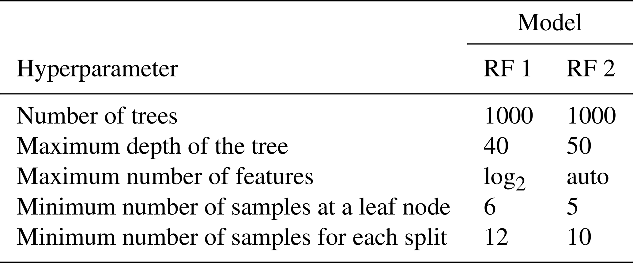
Table C1Meteorological variables used for training the random forest algorithm. The three types of feature are the measured meteorological variable, modelled meteorological variable by SNOWPACK, and extracted variable. Features can be discarded by recursive feature elimination (RFE), manually, or because they are highly correlated with another one.
Table C2Variables extracted from the simulated profiles used for training the random forest algorithm. Features can be discarded by recursive feature elimination (RFE) or because they are highly correlated with another one.
Here we provide a detailed description of the daily performance of the models on six selected dates that differed in terms of forecast agreement rate and model performance (Fig. D1). For simplicity, we only display the predictions of the model RF 1 (circles), for which we additionally provide a video in the Supplement. The maps of the predictions of the model RF 2 for these dates are also available in the Supplement. Also shown in Fig. D1 are the local nowcast assessments for each of these six dates (triangles).
Figure D1Maps of Switzerland showing the danger level of the public forecast for each region; the danger level predictions by the RF 1 model at each IMIS station (coloured circles); and the local nowcast assessments (coloured triangles) reported by observers on six selected dates – (a) 7 February 2019, (b) 15 March 2019, (c) 19 March 2019, (d) 20 January 2020, (e) 6 March 2020, and (f) 8 April 2020. The colours represent the danger levels.
On 7 February 2019 (Fig. D1a; denoted by “a” in Fig. 7a), danger level 3-Considerable was forecast for most regions. For this large area, the model predicted 2-Moderate for the majority of the stations, reaching a poor average daily accuracy of 0.3 (0.26 for RF 2). On this day, 27 observers provided a local assessment of the avalanche danger (Fig. D1a). A total of 8 assessments confirmed the forecast danger level 3-Considerable and 15 assessed the situation as 2-Moderate, suggesting that the forecast was likely too high in many regions (Pagree=0.41) and that the model actually performed well. In the remaining regions where the forecast danger level was 2-Moderate, the observers mostly confirmed the forecast (1 out of 4 reported 3-Considerable; Fig. D1a). The following day, the forecast danger level was lowered to 2-Moderate in almost all regions of the Swiss Alps.
On 15 March 2019 (Fig. D1b; denoted by “b” in Fig. 7a), danger levels 3-Considerable and 4-High were mainly forecast. The predictive accuracy on this day was 0.64 (0.62 for RF 2), considering the local nowcast assessments showed that the danger level forecast was perceived correctly by 17 out of 23 observers (Pagree=0.74). A total of 5 observers confirmed 4-High and 5 rated the danger with 3-Considerable in the area where the forecast danger level was 4-High. In the regions with forecast danger level 3-Considerable, 12 observers confirmed the forecast danger level and 1 reported 2-Moderate (Fig. D1b).
On 19 March 2019 (Fig. D1c; denoted by “c” in Fig. 7a), danger levels 2-Moderate and 3-Considerable were forecast. For a rather large proportion of the stations in the area with 2-Moderate, the model predicted one danger level higher, resulting in an average model accuracy of 0.53. For RF 2, overall accuracy was considerable higher, namely 0.65. Figure D1c shows that 79 % of the 24 local assessments on this day confirmed the forecast danger level: for 2-Moderate in 17 cases and for 3-Considerable in 2 out of 7 cases. This day seems to represent a typical example when RF 1, trained exclusively with forecast data, tended to predict higher danger levels than RF 2.
On 20 January 2020 (Fig. D1d; denoted by “d” in Fig. 7a), there were three areas with danger levels of 1-Low, 2-Moderate, and 3-Considerable, respectively. The average accuracy of the RF 1 model was 0.49, with many stations predicting a danger level of 2-Moderate in the area where 1-Low was forecast. Two local assessments on this day confirmed 1-Low, eight 2-Moderate, and two 3-Considerable, while four observers in the area where 3-Considerable was forecast rated the danger as 2-Moderate and one observer rated the area where 2-Moderate was forecast as 1-Low (Fig. D1d). In summary, this suggests that the forecast danger level was approximately correct (Pagree=0.7) but the model predictions tended to be too high, particularly in the area where 1-Low was forecast. The following day, the model predicted for most of the stations a decrease from 3-Considerable to 2-Moderate, now again in accordance with the forecast. The performance of RF 2 was better (overall accuracy of 0.61), showing more accurate predictions in the large area where danger level 1-Low was forecast (see video in the Supplement).
On 6 March 2020 (Fig. D1e; denoted by “e” in Fig. 7a), when primarily the danger level 3-Considerable was forecast, an accuracy of 0.81 was achieved by RF 1 (0.77 for RF 2). However, the feedback from the observers (Fig. D1e), with 15 out of the 27 local assessments being lower than the forecast danger level, suggests that the forecast danger level was at least in some regions too high (Pagree=0.46). Similarly, the avalanche observations indicated only for one warning region that level 4-High was appropriate.
Finally, on 8 April 2020 (Fig. D1f; denoted by “f” in Fig. 7a), the lowest danger level 1-Low was forecast for the entire area of the Swiss Alps. Both models also predicted 1-Low for all stations, an accuracy of 1. On this day, only four observers provided local nowcast estimates, all of which were in accordance with the forecast danger level (Fig. D1f).
The code to develop the final models used in this study is available at https://renkulab.io/gitlab/deapsnow/predictions_avalanche_danger-level_switzerland (Pérez-Guillén, 2022).
The data set of the meteorological and the profile variables extracted from the simulated profiles for each of the weather stations of the IMIS network in Switzerland and the danger ratings for dry-snow conditions assigned to the location of the station are accessible at https://doi.org/10.16904/envidat.330 (Pérez-Guillén et al., 2022).
For illustration, the evolution of the RF danger level predictions (circles), the local nowcast assessments (triangles), and the forecast danger level (Dforecast, Fig. 3d) is shown for the two test winters in two supplementary videos. Each video shows animations of the daily maps. Only the predictions for stations above the elevation indicated in the bulletin are displayed. The warning regions are coloured with the forecast danger level. The colour of the stations shows the danger level predictions of each random forest classifier. The number of stations varies with time because predictions at some stations are lacking due to (i) the station being located below the elevation indicated in the bulletin on a given day, (ii) a missing value for one of the input features, or (iii) the snow height being less than the minimum threshold of 30 cm. The danger level of some warning regions can also be missing for some days because only a forecast for wet-snow avalanche conditions was issued in this area. The supplement related to this article is available online at: https://doi.org/10.5194/nhess-22-2031-2022-supplement.
CP, FT, and MH processed the collection of the different data sources, developed the models, analysed the results, and prepared the manuscript with the contributions of all co-authors. MV, TO, GO, and FP provided the expertise for model choice and implementation, as well as assisting with handling large data volumes and the computational framework. JS, AV, and FT developed the research idea and aim of the study and reviewed the development of the models and manuscript.
The contact author has declared that neither they nor their co-authors have any competing interests.
Publisher's note: Copernicus Publications remains neutral with regard to jurisdictional claims in published maps and institutional affiliations.
Marc Ruesch and Mathias Bavay provided access to avalanche forecast and weather station data and to the SNOWPACK simulations. We would like to thank the editor, Pascal Haegeli, and the two referees, Pascal Hagenmuller and Karsten Müller, for their careful review and constructive comments that have contributed to improving our manuscript.
This project was funded by the Swiss Data Science Center under grant C18-05 “DEAPSnow”.
This paper was edited by Pascal Haegeli and reviewed by Karsten Müller and Pascal Hagenmuller.
Baggi, S. and Schweizer, J.: Characteristics of wet-snow avalanche activity: 20 years of observations from a high alpine valley (Dischma, Switzerland), Nat. Hazards, 50, 97–108, https://doi.org/10.1007/s11069-008-9322-7, 2009. a
Bavay, M. and Egger, T.: MeteoIO 2.4.2: a preprocessing library for meteorological data, Geosci. Model Dev., 7, 3135–3151, https://doi.org/10.5194/gmd-7-3135-2014, 2014. a
Bowler, N. E.: Explicitly accounting for observation error in categorical verification of forecasts, Mon. Weather Rev., 134, 1600–1606, https://doi.org/10.1175/MWR3138.1, 2006. a
Brabec, B. and Meister, R.: A nearest-neighbor model for regional avalanche forecasting, Ann. Glaciol., 32, 130–134, https://doi.org/10.3189/172756401781819247, 2001. a
Breiman, L.: Random forests, Mach. Learn., 45, 5–32, 2001. a
Bründl, M., Hafner, E., Bebi, P., Bühler, Y., Margreth, S., Marty, C., Schaer, M., Stoffel, L., Techel, F., Winkler, K., Zweifel, B., and Schweizer, J.: Ereignisanalyse Lawinensituation im Januar 2018, WSL Ber 76, WSL Institute for Snow and Avalanche Research – SLF, 162 pp., 2019. a, b, c
Bühler, Y., Hafner, E. D., Zweifel, B., Zesiger, M., and Heisig, H.: Where are the avalanches? Rapid SPOT6 satellite data acquisition to map an extreme avalanche period over the Swiss Alps, The Cryosphere, 13, 3225–3238, https://doi.org/10.5194/tc-13-3225-2019, 2019. a
Chen, C., Liaw, A., and Breiman, L.: Using random forest to learn imbalanced data, University of California, Berkeley, 110, 24, 2004. a
Davis, R. E., Elder, K., Howlett, D., and Bouzaglou, E.: Relating storm and weather factors to dry slab avalanche activity at Alta, Utah, and Mammoth Mountain, California, using classification and regression trees, Cold Reg. Sci. Technol., 30, 79–89, https://doi.org/10.1016/S0165-232X(99)00032-4, 1999. a
Dkengne Sielenou, P., Viallon-Galinier, L., Hagenmuller, P., Naveau, P., Morin, S., Dumont, M., Verfaillie, D., and Eckert, N.: Combining random forests and class-balancing to discriminate between three classes of avalanche activity in the French Alps, Cold Reg. Sci. Technol., 187, 103276, https://doi.org/10.1016/j.coldregions.2021.103276, 2021. a, b
Dreier, L., Harvey, S., van Herwijnen, A., and Mitterer, C.: Relating meteorological parameters to glide-snow avalanche activity, Cold Reg. Sci. Technol., 128, 57–68, https://doi.org/10.1016/j.coldregions.2016.05.003, 2016. a
EAWS: EAWS Matrix, Tech. rep., https://www.avalanches.org/standards/eaws-matrix/ (last access: 31 January 2020), 2017. a, b
EAWS: European Avalanche Danger Scale (2018/19), https://www.avalanches.org/standards/avalanche-danger-scale/ (last access: 18 June-2021), 2021a. a, b, c, d, e
EAWS: Information pyramid, https://www.avalanches.org/standards/information-pyramid/ (last access: 18 June 2021), 2021b. a
EAWS: Avalanche Problems, Edited, EAWS – European Avalanche Warning Services, https://www.avalanches.org/wp-content/uploads/2019/05/Typical_avalanche_problems-EAWS.pdf (last access: 18 June 2021), 2021c. a
Fierz, C., Armstrong, R. L., Durand, Y., Etchevers, P., Greene, E., McClung, D. M., Nishimura, K., Satyawali, P. K., and Sokratov, S. A.: The international classification for seasonal snow on the ground, https://unesdoc.unesco.org/ark:/48223/pf0000186462 (last access: 31 May 2022), 2009. a
Föhn, P. M. B.: The stability index and various triggering mechanisms, IAHS Publ., 162, 195–214, 1987. a, b
Föhn, P. M. B. and Schweizer, J.: Verification of avalanche danger with respect to avalanche forecasting, in: Les apports de la recherche scientifique à la sécurité neige glace et avalanche. Actes de Colloque, Chamonix, 30 mai–3 juin 1995, edited by: Sivardière, F., ANENA, Grenoble, France, 151–156, 1995. a
Frénay, B. and Verleysen, M.: Classification in the presence of label noise: a survey, IEEE T. Neural Netw. Learn. Syst., 25, 845–869, 2013. a
Gaume, J., van Herwijnen, A., Chambon, G., Wever, N., and Schweizer, J.: Snow fracture in relation to slab avalanche release: critical state for the onset of crack propagation, The Cryosphere, 11, 217–228, https://doi.org/10.5194/tc-11-217-2017, 2017. a
Guyon, I., Weston, J., Barnhill, S., and Vapnik, V.: Gene selection for cancer classification using support vector machines, Mach. Learn., 46, 389–422, 2002. a
Heck, M., Van Herwijnen, A., Hammer, C., Hobiger, M., Schweizer, J., and Fäh, D.: Automatic detection of avalanches combining array classification and localization, Earth Surf. Dynam., 7, 491–503, https://doi.org/10.5194/esurf-7-491-2019, 2019. a
Hendrikx, J., Murphy, M., and Onslow, T.: Classification trees as a tool for operational avalanche forecasting on the Seward Highway, Alaska, Cold Reg. Sci. Technol., 97, 113–120, https://doi.org/10.1016/j.coldregions.2013.08.009, 2014. a
Hendrikx, J., Dreier, L., Ulivieri, G., Sanderson, J., Jones, A., and Steinkogler, W.: Evaluation of an infrasound detection system for avalanches in Rogers Pass, Canada, in: Proceedings ISSW 2018, International Snow Science Workshop, 7–12 October 2018, Innsbruck, Austria, 171–175, 2018. a
Jamieson, B., Campbell, C., and Jones, A.: Verification of Canadian avalanche bulletins including spatial and temporal scale effects, Cold Reg. Sci. Technol., 51, 204–213, https://doi.org/10.1016/j.coldregions.2007.03.012, 2008. a
Jamieson, J. and Johnston, C.: Refinements to the stability index for skier-triggered dry-slab avalanches, Ann. Glaciol., 26, 296–302, https://doi.org/10.3189/1998AoG26-1-296-302, 1998. a, b, c
Kahneman, D., Sibony, O., and Sunstein, C. R.: Noise – A flaw in human judgment, Hachette Book Group, New York, USA, 454 pp., ISBN 10 0316451401, 2021. a
LaChapelle, E. R.: The fundamental processes in conventional Alavalanche forecasting, J. Glaciol., 26, 75–84, https://doi.org/10.3189/S0022143000010601, 1980. a, b
Lehning, M., Bartelt, P., Brown, B., Russi, T., Stöckli, U., and Zimmerli, M.: SNOWPACK model calculations for avalanche warning based upon a new network of weather and snow stations, Cold Reg. Sci. Technol., 30, 145–157, https://doi.org/10.1016/S0165-232X(99)00022-1, 1999. a, b, c, d
Lehning, M., Bartelt, P., Brown, B., Fierz, C., and Satyawali, P.: A physical SNOWPACK model for the Swiss avalanche warning: Part II. Snow microstructure, Cold Reg. Sci. Technol., 35, 147–167, https://doi.org/10.1016/S0165-232X(02)00073-3, 2002. a
Maas, A., Rottensteiner, F., and Heipke, C.: Using label noise robust logistic regression for automated updating of topographic geospatial databases., in: XXIII ISPRS Congress, Commission VII 3 (2016), 133–140. https://doi.org/10.5194/isprsannals-III-7-133-2016, 2016. a
Mayer, S., van Herwijnen, A., Ulivieri, G., and Schweizer, J.: Evaluating the performance of an operational infrasound avalanche detection system at three locations in the Swiss Alps during two winter seasons, Cold Reg. Sci. Technol., 173, 102962, https://doi.org/10.1016/j.coldregions.2019.102962, 2020. a
McClung, D. and Schaerer, P. A.: The avalanche handbook, The Mountaineers Books, ISBN 13 978-0898868098, 2006. a
McClung, D. M.: Predictions in avalanche forecasting, Ann. Glaciol., 31, 377–381, https://doi.org/10.3189/172756400781820507, 2000. a
Mitterer, C. and Schweizer, J.: Analysis of the snow-atmosphere energy balance during wet-snow instabilities and implications for avalanche prediction, The Cryosphere, 7, 205–216, https://doi.org/10.5194/tc-7-205-2013, 2013. a
Möhle, S., Bründl, M., and Beierle, C.: Modeling a system for decision support in snow avalanche warning using balanced random forest and weighted random forest, in: Lecture notes in computer science: Vol. 8722, Artificial intelligence: methodology, systems, and applications, Proceedings, edited by: Agre, G., Hitzler, P., Krisnadhi, A. A., and Kuznetsov, S. O., Springer, 80–91, https://doi.org/10.1007/978-3-319-10554-3_8, 2014. a
Monti, F., Schweizer, J., and Fierz, C.: Hardness estimation and weak layer detection in simulated snow stratigraphy, Cold Reg. Sci. Technol., 103, 82–90, https://doi.org/10.1016/j.coldregions.2014.03.009, 2014. a
Monti, F., Gaume, J., van Herwijnen, A., and Schweizer, J.: Snow instability evaluation: calculating the skier-induced stress in a multi-layered snowpack, Nat. Hazards Earth Syst. Sci., 16, 775–788, https://doi.org/10.5194/nhess-16-775-2016, 2016. a, b
Morin, S., Horton, S., Techel, F., Bavay, M., Coléou, C., Fierz, C., Gobiet, A., Hagenmuller, P., Lafaysse, M., Ližar, M., and Mitterer, C.,: Application of physical snowpack models in support of operational avalanche hazard forecasting: A status report on current implementations and prospects for the future, Cold Reg. Sci. Technol., 170, 102910, https://doi.org/10.1016/j.coldregions.2019.102910, 2020. a, b, c
Pedregosa, F., Varoquaux, G., Gramfort, A., Michel, V., Thirion, B., Grisel, O., Blondel, M., Prettenhofer, P., Weiss, R., Dubourg, V., and Vanderplas, J.: Scikit-learn: Machine learning in Python, J. Mach. Learn. Res., 12, 2825–2830, 2011. a
Pelletier, C., Valero, S., Inglada, J., Champion, N., Marais Sicre, C., and Dedieu, G.: Effect of training class label noise on classification performances for land cover mapping with satellite image time series, Remote Sens., 9, 173, https://doi.org/10.3390/rs9020173, 2017. a
Pérez-Guillén, C.: Data-driven automated predictions of the avalanche danger level for dry-snow conditions in Switzerland, Renkulab [code], https://renkulab.io/gitlab/deapsnow/predictions_avalanche_danger-level_switzerland, last access: 9 June 2022. a
Pérez-Guillén, C., Techel, F., Hendrick, M., Volpi, M., van Herwijnen, A., Olevski, T., Obozinski, G., Pérez-Cruz, F., and Schweizer, J.: Weather, snowpack and danger ratings data for automated avalanche danger level predictions, EnviDat [data set], https://doi.org/10.16904/envidat.330, 2022. a
Perla, R. I.: On contributory factors in avalanche hazard evaluation, Can. Geotech. J., 7, 414–419, https://doi.org/10.1139/t70-053, 1970. a
Pozdnoukhov, A., Purves, R. S., and Kanevski, M.: Applying machine learning methods to avalanche forecasting, Ann. Glaciol., 49, 107–113, https://doi.org/10.3189/172756408787814870, 2008. a
Pozdnoukhov, A., Matasci, G., Kanevski, M., and Purves, R. S.: Spatio-temporal avalanche forecasting with Support Vector Machines, Nat. Hazards Earth Syst. Sci., 11, 367–382, https://doi.org/10.5194/nhess-11-367-2011, 2011. a
Purves, R., Morrison, K., Moss, G., and Wright, D.: Nearest neighbours for avalanche forecasting in Scotland – development, verification and optimisation of a model, Cold Reg. Sci. Technol., 37, 343–355, https://doi.org/10.1016/S0165-232X(03)00075-2, 2003. a
Richter, B., Schweizer, J., Rotach, M. W., and van Herwijnen, A.: Validating modeled critical crack length for crack propagation in the snow cover model SNOWPACK, The Cryosphere, 13, 3353–3366, https://doi.org/10.5194/tc-13-3353-2019, 2019. a
Rodriguez-Galiano, V. F., Ghimire, B., Rogan, J., Chica-Olmo, M., and Rigol-Sanchez, J. P.: An assessment of the effectiveness of a random forest classifier for land-cover classification, ISPRS J. Photogram. Remote Sens., 67, 93–104, https://doi.org/10.1016/j.isprsjprs.2011.11.002, 2012. a
Schirmer, M., Lehning, M., and Schweizer, J.: Statistical forecasting of regional avalanche danger using simulated snow-cover data, J. Glaciol., 55, 761–768, https://doi.org/10.3189/002214309790152429, 2009. a, b
Schweizer, J.: Verifikation des Lawinenbulletins, in: Schnee und Lawinen in den Schweizer Alpen, Winter 2004/2005, Wetter, Schneedecke und Lawinengefahr, Winterbericht SLF, edited by: Pielmeier, C., Aebi, M., and Schweizer, J., Eidg. Institut für Schnee- und Lawinenforschung SLF, Davos, Switzerland, 91–99, 2007. a, b, c
Schweizer, J. and Föhn, P. M.: Avalanche forecasting – an expert system approach, J. Glaciol., 42, 318–332, https://doi.org/10.3189/S0022143000004172, 1996. a, b
Schweizer, J. and Jamieson, J. B.: A threshold sum approach to stability evaluation of manual snow profiles, Cold Reg. Sci. Technol., 47, 50–59, https://doi.org/10.1016/j.coldregions.2006.08.011, 2007. a
Schweizer, J., Föhn, P., and Plüss, C.: COGENSYS Judgment Processor (PARADOCS) als Hilfmittel für die Lawinenwarnung, Interner Bericht, Report No. 675, Eidgenössisches Institut für Schnee- und Lawinenforschung, https://www.dora.lib4ri.ch/wsl/islandora/object/wsl:30627 (last access: 9 June 2022), 1992. a
Schweizer, J., Jamieson, J. B., and Skjonsberg, D.: Avalanche forecasting for transportation corridor and backcountry in Glacier National Park (BC, Canada), in: 25 Years of Snow Avalanche Research, Voss, Norway, 12–16 May 1998, NGI Publication, Vol. 203, edited by: Hestnes, E., Norwegian Geotechnical Institute, Oslo, Norway, 238–243, 1998. a
Schweizer, J., Kronholm, K., and Wiesinger, T.: Verification of regional snowpack stability and avalanche danger, Cold Reg. Sci. Technol., 37, 277–288, https://doi.org/10.1016/S0165-232X(03)00070-3, 2003. a, b, c, d, e, f, g, h
Schweizer, J., Bellaire, S., Fierz, C., Lehning, M., and Pielmeier, C.: Evaluating and improving the stability predictions of the snow cover model SNOWPACK, Cold Reg. Sci. Technol., 46, 52–59, https://doi.org/10.1016/j.coldregions.2006.05.007, 2006. a
Schweizer, J., Mitterer, C., Techel, F., Stoffel, A., and Reuter, B.: On the relation between avalanche occurrence and avalanche danger level, The Cryosphere, 14, 737–750, https://doi.org/10.5194/tc-14-737-2020, 2020. a, b
Schweizer, J., Mitterer, C., Reuter, B., and Techel, F.: Avalanche danger level characteristics from field observations of snow instability, The Cryosphere, 15, 3293–3315, https://doi.org/10.5194/tc-15-3293-2021, 2021. a, b
Schweizer, M., Föhn, P. M. B., Schweizer, J., and Ultsch, A.: A hybrid expert system for avalanche forecasting, in: Information and Communications Technologies in Tourism, 12–14 January 1994, Innsbruck, Austria, 148–153, 1994. a, b
SLF: Avalanche bulletin interpretation guide, WSL Institute for Snow and Avalanche Research – SLF, edition December 2020, p. 53, https://www.slf.ch/files/user_upload/SLF/Lawinenbulletin_Schneesituation/Wissen_zum_Lawinenbulletin/Interpretationshilfe/Interpretationshilfe_EN.pdf (last access: 2 June 2022), 2020. a, b
Sokolova, M. and Lapalme, G.: A systematic analysis of performance measures for classification tasks, Inform. Process. Manage., 45, 427–437, 2009. a
Statham, G., Haegeli, P., Greene, E., Birkeland, K., Israelson, C., Tremper, B., Stethem, C., McMahon, B., White, B., and Kelly, J.: A conceptual model of avalanche hazard, Nat. Hazards, 90, 663–691, https://doi.org/10.1007/s11069-017-3070-5, 2018. a, b
Strobl, C., Boulesteix, A.-L., Zeileis, A., and Hothorn, T.: Bias in random forest variable importance measures: Illustrations, sources and a solution, BMC Bioinf., 8, 1–21, https://doi.org/10.1186/1471-2105-8-25, 2007. a
Techel, F.: On consistency and quality in public avalanche forecasting: a data-driven approach to forecast verification and to refining definitions of avalanche danger, PhD thesis, Department of Geography, University of Zurich, Zurich, Switzerland, https://doi.org/10.5167/uzh-199650, 2020. a, b, c, d, e
Techel, F. and Schweizer, J.: On using local avalanche danger level estimates for regional forecast verification, Cold Reg. Sci. Technol., 144, 52–62, https://doi.org/10.1016/j.coldregions.2017.07.012, 2017. a, b, c, d, e, f, g, h, i, j, k, l, m, n, o, p, q
Techel, F., Zweifel, B., and Winkler, K.: Analysis of avalanche risk factors in backcountry terrain based on usage frequency and accident data in Switzerland, Nat. Hazards Earth Syst. Sci., 15, 1985–1997, https://doi.org/10.5194/nhess-15-1985-2015, 2015. a
Techel, F., Müller, K., and Schweizer, J.: On the importance of snowpack stability, the frequency distribution of snowpack stability and avalanche size in assessing the avalanche danger level, The Cryosphere, 14, 3503–3521, https://doi.org/10.5194/tc-2020-42, 2020a. a, b, c
Techel, F., Pielmeier, C., and Winkler, K.: Refined dry-snow avalanche danger ratings in regional avalanche forecasts: Consistent? And better than random?, Cold Reg. Sci. Technol., 180, 103162, https://doi.org/10.1016/j.coldregions.2020.103162, 2020b. a, b, c
Techel, F., Mayer, S., Pérez-Guillén, C., Schmudlach, G., and Winkler, K.: On the correlation between a sub-level qualifier refining the danger level with observations and models relating to the contributing factors of avalanche danger, Nat. Hazards Earth Syst. Sci., 22, 1911–1930, https://doi.org/10.5194/nhess-22-1911-2022, 2022. a
van Herwijnen, A., Heck, M., and Schweizer, J.: Forecasting snow avalanches using avalanche activity data obtained through seismic monitoring, Cold Reg. Sci. Technol., 132, 68–80, https://doi.org/10.1016/j.coldregions.2016.09.014, 2016. a
Wever, N., Fierz, C., Mitterer, C., Hirashima, H., and Lehning, M.: Solving Richards Equation for snow improves snowpack meltwater runoff estimations in detailed multi-layer snowpack model, The Cryosphere, 8, 257–274, https://doi.org/10.5194/tc-8-257-2014, 2014. a
Winkler, K., Schmudlach, G., Degraeuwe, B., and Techel, F.: On the correlation between the forecast avalanche danger and avalanche risk taken by backcountry skiers in Switzerland, Cold Reg. Sci. Technol., 188, 103299, https://doi.org/10.1016/j.coldregions.2021.103299, 2021. a, b
Zweifel, B., Hafner, E., Lucas, C., Marty, C., Techel, F., and Stucki, T.: Schnee und Lawinen in den Schweizer Alpen. Hydrologisches Jahr 2018/19, WSL Ber. 86, WSL-Institut für Schnee- und Lawinenforschung – SLF, Davos, 134 pp., https://www.dora.lib4ri.ch/wsl/islandora/object/wsl:22232 (last access: 2 June 2022), 2019. a, b, c
- Abstract
- Introduction
- Data
- Data preparation
- Model optimization
- Model evaluation
- Discussion
- Conclusions
- Appendix A: Compilation of subset of tidy danger levels (Dtidy)
- Appendix B: Metrics and model's hyperparameters
- Appendix C: Definition of features for developing RF models
- Appendix D: Illustrative case studies
- Code availability
- Data availability
- Author contributions
- Competing interests
- Disclaimer
- Acknowledgements
- Financial support
- Review statement
- References
- Supplement