Hidden-state modeling of a cross-section of geoelectric time series data can provide reliable intermediate-term probabilistic earthquake forecasting in Taiwan

Geoelectric time series (TS) have long been studied for their potential for probabilistic earthquake forecasting, and a recent model (GEMSTIP) directly used the skewness and kurtosis of geoelectric TS to provide times of increased probability (TIPs) for earthquakes for several months in the future. We followed up on this work by applying the hidden Markov model (HMM) to the correlation, variance, skewness, and kurtosis TSs to identify two hidden states (HSs) with different distributions of these statistical indexes. More importantly, we tested whether these HSs could separate time periods into times of higher/lower earthquake probabilities. Using 0.5 Hz geoelectric TS data from 20 stations across Taiwan over 7 years, we first computed the statistical index TSs and then applied the Baum–Welch algorithm with multiple random initializations to obtain a well-converged HMM and its HS TS for each station. We then divided the map of Taiwan into a 16-by-16 grid map and quantified the forecasting skill, i.e., how well the HS TS could separate times of higher/lower earthquake probabilities in each cell in terms of a discrimination power measure that we defined. Next, we compare the discrimination power of empirical HS TSs against those of 400 simulated HS TSs and then organized the statistical significance values from this cellular-level hypothesis testing of the forecasting skill obtained into grid maps of discrimination reliability. Having found such significance values to be high for many grid cells for all stations, we proceeded with a statistical hypothesis test of the forecasting skill at the global level to find high statistical significance across large parts of the hyperparameter spaces of most stations. We therefore concluded that geoelectric TSs indeed contain earthquake-related information and the HMM approach is capable of extracting this information for earthquake forecasting.

1 Introduction

Earthquakes (EQs) are one of the most destructive natural hazards that can befall us, with the potential to take many human lives and cause serious damage to economies and environments. It is imperative for us to work towards better forecasting/prediction capabilities against EQs, to inform pre-EQ evacuation and post-EQ relief, as well as expediting critical reinforcement works for selected buildings and infrastructures. To achieve this goal, the scientific community has done much work discovering precursors and models that are useful for the forecasting/prediction of EQs.

First, let us clarify that in the seismological community, the terms “prediction” and “forecast” are often used interchangeably (Kagan, 1997; Ismail-Zadeh, 2013). When they are distinguished, the term prediction emphasizes the issuing of an alarm with high accuracy and reliability indicating the time, location, and magnitude of the next large EQ (Geller et al., 1997), whereas the term forecast is a statement about the probability of EQs within the specified spatial–temporal window (Ismail-Zadeh, 2013). Till this day, it is extremely difficult to make accurate and specific EQ predictions (Geller et al., 1997). However, the forecasting of EQs is a far more tractable task: a method that performs better than random guesses (the null hypothesis) is recognized as having predictive power or predictive skill (prediction and forecast used as synonyms here) (Kagan, 1997). In this paper, we will also use the two terms interchangeably.

If we categorize EQ forecasting methods according to their timescales, we can organize them into three categories: long-term (decades ahead), intermediate-term (a few years ahead), and short-term (days or a few months ahead) (Peresan et al., 2005; Kanamori, 2003). EQ forecasting at different timescales serves different purposes. For a region of interest, long-term EQ forecasting aims to estimate the probabilities of large EQs in the next decades or more. In most past studies, the primary input data were from the historical EQ catalog, which allowed statistical modeling of the occurrence times of large- and medium-sized EQs (Kagan and Jackson, 1994; Sykes, 1996; Papazachos et al., 1987; Papadimitriou, 1993; Papazachos et al., 1997), assuming that EQs' occurrences in the same spatial area follow a Poisson process of a relatively constant rate. One such example is the probabilistic seismic hazard assessment (PSHA) first established by Cornell in 1968 (Cornell, 1968). This became a popular method for long-term seismic hazard assessment implemented in many countries (Tavakoli and Ghafory-Ashtiany, 1999; Petersen, 1996; Meletti et al., 2008; Vilanova and Fonseca, 2007; Nath and Thingbaijam, 2012; Wang et al., 2016). In this method, we take into account both historical EQ catalog information and ground motion characteristics for the modeling of energy attenuation over spatial distances, thus providing a map of seismic hazard rates that varies across location for the next 50 years. Long-term EQ forecasting such as PSHA can be valuable for location-specific seismic risk evaluation, thereby providing guidelines or criteria for local construction projects. For example, a building that is expected to last 100 years must be able to withstand 10 large EQs of the magnitude that occurs once every 10 years locally. What long-term EQ forecasting cannot do is tell people how to do things differently at any time.

For intermediate-term EQ forecasting, the aim is to detect deviations of EQ rates from their long-term values to assess increased probabilities of EQs within the next 1 to 10 years. For example, if a region usually has a magnitude 6 EQ every 10 years and 15 years have passed without one, the region would be in a state of increased probability. A famous example of intermediate-term EQ forecasting is the M8 algorithm (Kossobokov et al., 2002; Peresan et al., 2005; Keilis-Borok, 1996), developed by Healy et al. (1992). The M8 algorithm used the EQ catalog as input and returned as output the time of increased probability (TIP) for EQs of magnitude 7.5 and above for the next 1 year. Another example is the CN algorithm (Peresan et al., 2005; Keilis-Borok, 1996) developed by Keilis-Borok and Rotwain (1990), which also took the EQ catalog as input to produce as output the TIP for strong EQs (defined specifically for different regions) within the next half year to a few years. In the literature, we also found the self-organizing spinodal (SOS) model (Chen, 2003; Rundle et al., 2000), which used the increased activity of medium-sized EQs as precursors to large EQs that could occur within the next several years or decades. Finally, one of the more successful methods at this timescale is pattern informatics (Nanjo et al., 2006), which was demonstrated to be effective at predicting M≥5 EQs in Japan between 2000 and 2009. Intermediate-term EQ forecasting can, for example, help local authorities prioritize inspections and reinforcements of old buildings over the construction of new ones.

Short-term EQ forecasting uses a variety of methods to forecast the time, place, and magnitude of a specific large EQ. Here we commonly find methods using the EQ catalog as input data and apply machine learning approaches (Asim et al., 2017; Reyes et al., 2013), as well as hidden Markov model (HMM) approaches (Yip et al., 2018; Chambers et al., 2012). For example, in Chambers et al. (2012) an HMM was trained to track the waiting time between EQs with magnitudes above 4 in southern California and western Nevada (Yip et al., 2018), giving EQ forecasts for up to 10 d in the future. Apart from using EQ catalog data, there are an increasing variety of methods using other data inputs, such as the widely used seismic electric signals (SESs) (Uyeda et al., 2000; Varotsos et al., 2002, 2013, 2017; Varotsos and Lazaridou, 1991; Varotsos et al., 1993), to look for EQ precursors in the form of abnormal changes to the geoelectric potential. In addition to looking for specific SES-type precursors, we also found papers using methods such as artificial neural networks (ANNs) (Moustra et al., 2011), Fisher information (Telesca et al., 2005a, 2009;), and multi-fractal analysis (Telesca et al., 2005b) directly on geoelectric time series (TS) data to make short-term EQ forecasting. Other data that can be used include the combination of geoelectric and magnetic data (Kamiyama et al., 2016; Sarlis, 2018), GPS crustal movements (Kamiyama et al., 2016; Wang and Bebbington, 2013), electromagnetics of the atmosphere (Hayakawa and Hobara, 2010), and lithosphere dynamics (Shebalin et al., 2006). Short-term EQ forecasting can guide emergency responses such as evacuations and preemptive relief efforts, although it is usually not reliable enough based on our current level of understanding.

Among all these precursors, our recent research interest has been in the potential use of geoelectric TSs for EQ forecasting (Chen and Chen, 2016; Chen et al., 2020; Jiang et al., 2020; Telesca et al., 2014; Chen et al., 2017). In 2016 and 2017, Chen and his colleagues (Chen and Chen, 2016; Chen et al., 2017) analyzed the data of 20 geoelectric stations in Taiwan (Fig. 1) and studied the association between skewness and kurtosis of the geoelectric data and M_L≥ 5 EQs, where M_L is the Richter magnitude scale. Through statistical analyses, they found significant correlations between geoelectric anomalies and these large EQs. They then developed an EQ forecasting algorithm named GEMSTIP to extract TIPs for future EQs. TIPs were identified through differences in the distributions of skewness and kurtosis from those found during normal periods. Moreover, Jiang et al. (2020) investigated the geoelectric signals before, during, and after EQs by the shifting correlation method and found that the lateral and vertical electrical resistivity variation and subsurface conductors might amplify SESs, which agreed with the findings by Sarlis et al. (1999) and Huang and Lin (2010).

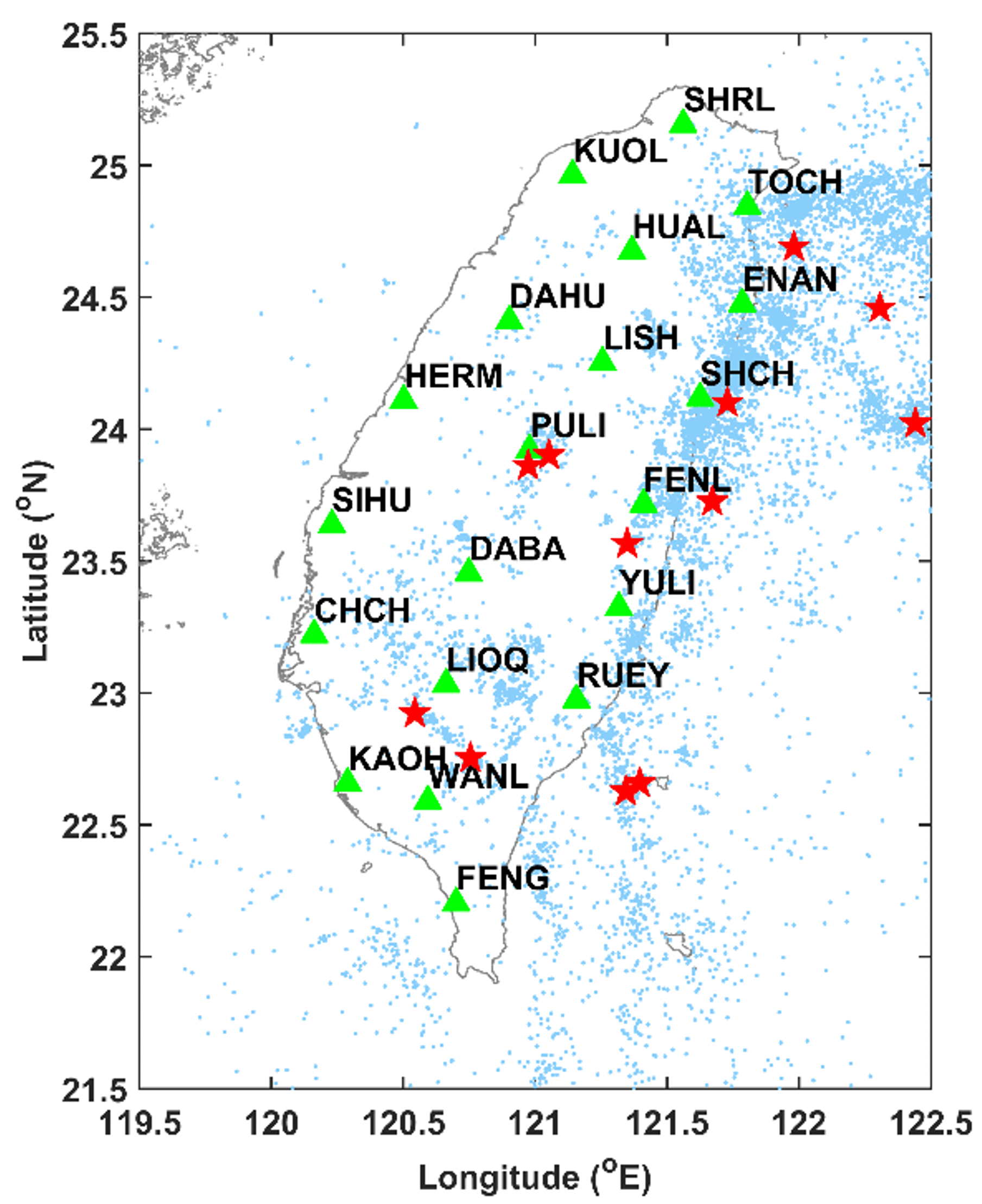
Figure 1 Map of the spatial distributions of seismicity and geoelectric stations (green triangles) in Taiwan. In this figure, past EQs with M_L≥3 are shown as light blue dots and past EQs with M_L≥6 are shown as red stars.

Inspired by these findings, in this paper we wanted to take a closer look at the relationship between the EQ times and statistical indexes of geoelectric TSs, namely correlation (C), variance (V), skewness (S), and kurtosis (K). During initial explorations, we computed the TSs of these indexes (see Sect. 2.2 for computation details) on geoelectric TSs given by the 20 stations over the 7-year period of January 2012–December 2018 (see Sect. 2.1 for data details). We then aggregated the distribution of the indexes' values within different time-to-failure (TTF, i.e., time remaining to the next EQ) intervals. In Fig. 2, we show the normalized frequency distributions of C, V, S, and K computed from the KAOH station at different TTFs (using 0.9 d intervals) for M_L≥4 EQs within 2^∘ longitude and latitude of the KAOH station. In this figure, we see bands of darker-colored pixels across the TTFs. Specifically, for C, V, and S, there are sudden shifts in the average position of the bands, suggesting that there are two regimes (short TTFs and long TTFs) where the geoelectric fields show qualitatively different behaviors. For all statistical indexes, we find the darkest pixels concentrated in the long-TTF regime, whereas in the short-TTF regime, the pixels show a lower variability in their intensities. We suspect that this second phenomenon is the result of fewer samples at longer TTFs.

Figure 2 Heatmaps of normalized probability density functions of C, V, S, and K at different times to failure (TTFs), for the east–west component of the geoelectric TS. The TTFs are computed using M_L≥4 EQs within 2^∘ longitude and latitude of the KAOH station.

To overcome this problem, which is created by superimposing the index TSs of different lengths between EQs, we decided to discover such regimes directly from the geoelectric TSs by using HMMs. The HMM is well known for being data-driven, enabling us to search for and use more general statistical features beyond limited templates that we currently know (Beyreuther and Wassermann, 2008). Additionally, its explicit incorporation of the time dimension into the model is a distinct advantage for providing holistic and time-sensitive representations, especially in the application of EQ forecasting (Beyreuther and Wassermann, 2008). In our HMM, we defined two hidden states (HSs) as the high-level representations of geoelectricity, featuring unique distributions of C, V, S, and K. Here we chose to use only two, instead of more, HSs because two-state HMMs have already been successfully applied to model regimes with different EQ frequencies using EQ catalogs as the only inputs (Yip et al., 2018; Chambers et al., 2012). Thereafter, for each monitoring station, we obtained the TS of posterior HS probability, or HS TS, using the TSs of C, V, S, and K and the Baum–Welch algorithm (BWA). We then partitioned the time periods under study according to the HS TSs and investigated whether these HS TSs that are obtained purely from geoelectric data can separate time periods of high versus low EQ (M_L≥3) probabilities, with high statistical confidence.

The goal of this investigation is to decide whether the hidden Markov modeling of geoelectric TSs could provide features (i.e., HS TSs) of true forecasting skill for intermediate-term EQ forecasting. Therefore, we are more concerned with statistical significance than with evaluating the exact forecasting accuracy or with the forecasting of specific EQs. In this regard, we also note that the same HMM approach described in this paper can be applied to many other geophysical high-frequency time series data, such as geomagnetic or GPS ground movement data, even though we only used geoelectric data as the input of the HMM, to show that the underlying seismic dynamics is indeed clearly separable into distinct regimes of higher versus lower seismic activities (as supported by Yip et al., 2018; Chambers et al., 2012).

For the sake of our readers, we organize our “Data and methods” in Sect. 2, “Results and discussions” in Sect. 3, and Conclusions in Sect. 4. In Sect. 2, we provide information on the EQ catalog; the geoelectric TSs; and how we pre-processed the latter and subsequently computed the index TSs of C, V, S, and K from them. We then explain how an HMM and the Baum–Welch algorithm works, before applying them to our problem. We also explain why we did not estimate individual HMMs from the index TSs of C, V, S, and K but one HMM for each station from an observation TS aggregating C, V, S, and K through k-means clustering. At the end of this section, we present our procedures for quantifying how informative the HSs are against EQ activities, by defining and analyzing EQ grid maps, EQ frequencies, and EQ frequency ratios (R_F). In Sect. 3, we first used the R_F grid map of 1 of the 20 stations to illustrate how we can compare a discrimination power (D) grid map against 400 simulated grid maps of D to obtain the discrimination reliability (R_D) grid map, which comprises cellular-level statistical significances that the HSs are useful for EQ forecasting. We then performed significance tests to verify that the HSs' forecasting power is also significant at the global level, using a metric of the global confidence level (GCL) that we defined. To end Sect. 3, we explored how robust the GCL values are across the hyperparameter space and clarified how we chose the optimal hyperparameters for each station. Finally, we conclude in Sect. 4.

2 Data and methods

2.1 Data description

The 1 Hz geoelectric TSs data used in this paper were provided by the 20 monitoring stations located across Taiwan (see Fig. 1), which are collectively named the Geoelectric Monitoring System (GEMS). The spacing between stations is generally 50 km. The geoelectric data here are the self-potential data, which are the natural electric potential differences in the earth, measured by dipoles placed 1–4 km apart within each station. Each station can output two sets of high-frequency geoelectric TSs, measuring separately the NS direction and the EW direction. Depending on the spatial constraints of some stations, the azimuths of the dipoles might deviate from the exact NS or EW directions by 10–40^∘. For the purpose of this study, we used the geoelectric TSs provided by GEMS with the same time span as the EQ catalog data, which is from January 2012 to December 2018. We downsampled the data to 0.5 Hz and used these in subsequent analyses.

The HMMs that we will show in Sect. 3 partitioned the 20 geoelectric TSs into two HSs, distinguished by the local statistics of their geoelectric fields. We believe these HSs can also exhibit different seismicity within their time durations. To check this, we used EQ catalog data compiled by the Central Weather Bureau (CWB), in charge of monitoring EQs in the region of Taiwan (Shin et al., 2013). The CWB seismic network is highly dense and provides an abundant set of waveform data. Due to the considerable EQs recorded, the seismotectonics of Taiwan is well depicted, showing the complicated subduction between the Philippine Sea and Eurasian plates (Kuo-Chen et al., 2012; Yi-Ben, 1986). Despite the dense seismic network, the EQ catalog was shown to be incomplete at small magnitudes due to the detection threshold of seismic instruments and the coverage of networks (Fischer and Bachura, 2014; Nanjo et al., 2010; Rydelek and Sacks, 1989). In Taiwan, the completeness magnitude (M_c), defined as the lowest magnitude above which all EQs are reliably detected, is approximately between 2 and 3 (Chen et al., 2012; Mignan et al., 2011). Chen et al. (2012) showed the temporal variation in M_c, while Mignan et al. (2011) provided the spatial information of that. In this study, for a conservative estimate, we took the completeness magnitude of 3 and analyzed EQs with M_L≥3, during the period from January 2012 to December 2018 in the area of 119.5–122.5^∘ E and 21.5–25.5^∘ N, as shown in Fig. 1, in which the locations of strong events with M_L≥6 are marked. Some of these events were destructive. For instance, at 03:57 on 6 February 2016 (UTC+8), an M_L 6.6 EQ occurred in the southern part of Taiwan (22.92^∘ N, 120.54^∘ E). This event struck at a depth of around 14.6 km (Chen et al., 2017; Lee et al., 2016; Pan et al., 2019). Such a comparatively shallow depth caused more intensities on the surface and resulted in widespread damage which included 117 deaths and over 500 wounded.

In the latest update of the GEMSTIP model, Chen et al. (2021) found that by applying a specific bandpass filter to the geoelectric TS, the model became better at anticipating EQs using the skewness and kurtosis TSs. The filter they used is the third-order Butterworth bandpass filter with lower and higher cutoff frequencies of $f_{\mathrm{1}}={\mathrm{10}}^{-\mathrm{4.0}}$ and $f_{\mathrm{2}}={\mathrm{10}}^{-\mathrm{1.75}}$ Hz respectively. These lower and upper cutoff frequencies were determined by Chen et al. (2021) to give the optimal signal-to-noise ratio.

Similarly to the GEMSTIP model, our hidden Markov modeling also searched for EQ-related information in skewness and kurtosis TSs computed from the geoelectric TS; we conveniently utilized the insight from Chen et al. (2021) and applied the same Butterworth filter to our geoelectric TS data before computing the index TSs. This filter was applied using the scipy.signal (v1.4.1) package in Python (v3.6.5), with instructions from the SciPy Cookbook (2012), which also demonstrated a clear working example of the Butterworth bandpass filter that readers can refer to.

2.2 Computation of index TSs of C, V, S, and K

For each station, there are two geoelectric TSs (NS and EW) of frequency 0.5 Hz. Each geoelectric TS will produce four statistical index TSs (C, V, S, K). For each station, we therefore obtained up to eight index TSs, four for each direction (NS and EW). Starting from the 0.5 Hz geoelectric TS, we computed one index point for every non-overlapping time window of length L_w geoelectric TS data points. Later in Sect. 3.5, we will discuss in detail how we chose the optimal L_w individually for each station in the parameter space that we tested: {0.02, 0.03, 0.04, 0.05, 0.1, 0.2, 0.25} (d). As can be noticed from Fig. 12, 11 out of 20 stations' optimal choice was L_w=0.02 or L_w=0.03 d, which we suppose can be a good compromise between timely monitoring of state shifts and updating at a comfortable frequency for the human decision makers. Potential decisions that such an update frequency may enable include the forward deployment of relief materials such as backup generators, portable water treatment units, tents, medical supplies, and refresher training of emergency response teams, as well as administrative prioritizing of re-certification works for buildings and structures in regions where more EQs are expected soon.

Next, we present the definitions for each index. Within each time window, let us write the geoelectric field as ${\left\{X_n\right\}}_{n=\mathrm{1},\mathrm{\dots },L_{\mathrm{w}}}$. The correlation C that we used in this paper is the lag-1 Pearson autocorrelation of ${\left\{D_n=X_{n+\mathrm{1}}-X_n\right\}}_{n=\mathrm{1},\mathrm{\dots },L_{\mathrm{w}}-\mathrm{1}}$, which is the difference sequence of ${\left\{X_n\right\}}_{n=\mathrm{1},\mathrm{\dots },L_{\mathrm{w}}}$. Mathematically,

$$\begin{array}{}\text{(1)}& C\left(\left\{X_n\right\}\right)=AC\mathrm{1}\left(\left\{D_n\right\}\right)={\displaystyle \frac{\mathbb{E}\left[\left(D_n-{\mathit{\mu }}_D\right)\left(D_{n+\mathrm{1}}-{\mathit{\mu }}_D\right)\right]}{{\mathit{\sigma }}_{\mathrm{D}}^{\mathrm{2}}}},\end{array}$$

where E is the expectation, μ_D is the mean of ${\left\{D_n\right\}}_{n=\mathrm{1},\mathrm{\dots },L_{\mathrm{w}}-\mathrm{1}}$, and σ_D is the standard deviation of ${\left\{D_n\right\}}_{n=\mathrm{1},\mathrm{\dots },L_{\mathrm{w}}-\mathrm{1}}$. The range of C is [$-\mathrm{1},\mathrm{1}$], and C measures how fast the TS relaxes back to the equilibrium. If C is close to 1, X tends to increase or decrease persistently; if C is around 0, X is equivalent to random walks; and if C is close to −1, every increase in X would tend to be followed by a similar decrease.

The variance V of ${\left\{X_n\right\}}_{n=\mathrm{1},\mathrm{\dots },L_{\mathrm{w}}}$ is the sequence's second standard central moment. It is a positive number that measures how drastically the values in the sequence are different from each other, with higher values indicating higher difference. It is defined as

$$\begin{array}{}\text{(2)}& V\left(\left\{X_n\right\}\right)=\mathbb{E}\left[(X_n-{\mathit{\mu }}_X{)}^{\mathrm{2}}\right],\end{array}$$

where μ_X is the mean of ${\left\{X_n\right\}}_{n=\mathrm{1},\mathrm{\dots },L_{\mathrm{w}}}$. Additionally, we observed astronomically extreme values in the V TSs for most stations, which were caused by unknown technical errors, and we therefore considered them outliers that have to be removed for consistent data quality. We discuss how we removed them in detail in Supplement Sect. S1. From here onwards, the V TSs will always refer to those after the outlier-removal process.

The skewness S of ${\left\{X_n\right\}}_{n=\mathrm{1},\mathrm{\dots },L_{\mathrm{w}}}$, or the sequence's third standard central moment, is defined as

$$\begin{array}{}\text{(3)}& S\left(\left\{X_n\right\}\right)=\mathbb{E}\left[{\left({\displaystyle \frac{X_n-{\mathit{\mu }}_X}{{\mathit{\sigma }}_X}}\right)}^{\mathrm{3}}\right],\end{array}$$

where σ_X is the standard deviation of ${\left\{X_n\right\}}_{n=\mathrm{1},\mathrm{\dots },L_{\mathrm{w}}}$. It is a real number measuring how asymmetric the distribution of ${\left\{X_n\right\}}_{n=\mathrm{1},\mathrm{\dots },L_{\mathrm{w}}}$ is about the mean. For a perfectly symmetric distribution such as the normal distribution, the skewness is 0. A positive skewness means the distribution has a longer tail to the right, and a negative skewness means the distribution has a longer tail to the left.

The kurtosis K of ${\left\{X_n\right\}}_{n=\mathrm{1},\mathrm{\dots },L_{\mathrm{w}}}$, or the sequence's fourth standard central moment, is defined as

$$\begin{array}{}\text{(4)}& K\left(\left\{X_n\right\}\right)=\mathbb{E}\left[{\left({\displaystyle \frac{X_n-{\mathit{\mu }}_X}{{\mathit{\sigma }}_X}}\right)}^{\mathrm{4}}\right].\end{array}$$

It is a real number measuring how frequently extreme values (values very far from the mean) appear in the distribution. The higher the number, the more frequently extreme values can be found. As a reference, the kurtosis of the normal distribution is K=3. If K>3, we say that the distribution is leptokurtic, meaning the distribution has fatter tails and more frequent extreme values compared to the normal distribution. If K<3, the distribution is said to be platykurtic, meaning the distribution has thinner tails and extreme values appear less frequently compared to the normal distribution.

2.3 Estimation of the HMM using the Baum–Welch algorithm

A Markov model is a stochastic model that can be used to describe a system whose future state s_t+1 is drawn from a set of L states ${\left\{S_l\right\}}_{l=\mathrm{1},\mathrm{\dots },L}$ with probabilities $p_{j\leftarrow i}=P\left(s_{t+\mathrm{1}}=S_j\mathrm{|}{s}_t=S_i\right)$ conditioned by its current state s_t. The probabilities p_j←i can be organized into a transition matrix A, where $\mathbf{A}\left(i,j\right)=p_{j\leftarrow i}$. The HMM is an extension of the Markov model, with the additional property that the system state s_t is not explicitly known, hence the word “hidden” in the name. Instead, what can be observed from an HMM at any time t is an observable o_t drawn from a size-Q observable set ${\left\{O_q\right\}}_{q=\mathrm{1},\mathrm{\dots },Q}$. Just as in a Markov model, the future state s_t+1 of an HMM is drawn from the set ${\left\{S_l\right\}}_{l=\mathrm{1},\mathrm{\dots },L}$ with probabilities p_j←i (similarly conditioned by the current state s_t) taken from the transition matrix A. At time t, the observable o_t is emitted with a probability $P(o_t=O_q\mathrm{|}{s}_t=S_l)$ that depends on which HS s_t=S_l the system is in. These probabilities can be organized into an L×Q emission matrix B, where $\mathbf{B}\left(l,k\right)=P(o_t=O_q\mathrm{|}{s}_t=S_l)$. Additionally, we call the HS probability distributions at the initial time ${\mathit{\pi }}_{\mathrm{0}}=\left[P\left(S_{\mathrm{1}}\right),P\left(S_{\mathrm{2}}\right),\mathrm{\dots },P\left(S_L\right)\right]$. With this, we have fully specified the HMM: the sets of HSs ${\left\{S_l\right\}}_{l=\mathrm{1},\mathrm{\dots },L}$ and observations ${\left\{O_q\right\}}_{q=\mathrm{1},\mathrm{\dots },Q}$ as well as the model parameters that are collectively called $\mathit{\lambda }=\left(\mathbf{A},\mathbf{B},{\mathit{\pi }}_{\mathrm{0}}\right)$.

In common real-world applications of the HMM, the question is to estimate the probability distributions of the HS TS given the observation TS and the model parameter, namely $P(s_t=S_l\mathrm{|}{\left\{o_t\right\}}_{t=\mathrm{1},\mathrm{\dots },T}\mathit{\lambda })$. More often than not, the model parameter λ is unknown and has to be simultaneously estimated as well. One of the most common ways to do this is the Baum–Welch algorithm (BWA) (Zhang et al., 2014; Oudelha and Ainon, 2010; Yang et al., 1995; Bilmes, 1998), which belongs to the family of expectation maximization methods (Bilmes, 1998). Starting from randomly initialized model parameters λ, the algorithm runs recursively to maximize the likelihood of the model given the observation TS. When the algorithm converges, we will obtain a set of estimated model parameters $\stackrel{\mathrm{̃}}{\mathit{\lambda }}=\left(\stackrel{\mathrm{̃}}{\mathbf{A}},\stackrel{\mathrm{̃}}{\mathbf{B}},{\stackrel{\mathrm{̃}}{\mathit{\pi }}}_{\mathrm{0}}\right)$, as well as a posterior probability $P(s_t=S_l\mathrm{|}{\left\{o_t\right\}}_{t=\mathrm{1},\mathrm{\dots },T}\stackrel{\mathrm{̃}}{\mathit{\lambda }})$ TS. We include more details on the BWA in Sect. 2.5. Additionally, for readers who want an intuitive demonstration of how the HMM and BWA work, we have included a simulation of a simple HMM and its BWA application in Sect. S2.

HMMs are traditionally applied in fields such as speech recognition (Palaz et al., 2019; Novoa et al., 2018; Chavan and Sable, 2013; Abdel-Hamid and Jiang, 2013), bioinformatics, and anomaly detection (Qiao et al., 2002; Joshi and Phoha, 2005; Cho and Park, 2003). It has also been used for short-term EQ forecasting, using observations from EQ catalogs (Yip et al., 2018; Chambers et al., 2012; Ebel et al., 2007), as well as GPS measurements of ground deformations (Wang and Bebbington, 2013). To the best of our knowledge, there is no past HMM study on geoelectric TSs for EQ forecasting. In this paper, we argue that the HMM is an objective tool because the HSs were estimated only from the geoelectric TSs and thereafter validated against the EQ catalog. We believe this statistical procedure limits the bias that we could introduce into our prediction model when we optimized the model. This will be even clearer by the end of Sect. 2.5 where we summarize the entire procedure.

2.4 Hidden Markov modeling and inputs to the BWA

In the context of this study, we assume for simplicity two seismicity states of the earth crust beneath each station. These are our HSs {S₁, S₂} since they cannot be directly observed. What we can observe directly are the geoelectric TSs for each station. Our goal is to reconstruct the HS TSs so that the distributions of indexes (C, V, S, K) of the geoelectric TSs in S₁ and S₂ are as different as possible. To do this, we computed four index TSs each for NS and EW geoelectric fields using the procedure described in Sect. 2.2 and organized them into a TS of 8-dimensional feature vectors ${\mathit{F}}_t=\left(C_{\mathrm{NS},t},V_{\mathrm{NS},t},S_{\mathrm{NS},t},K_{\mathrm{NS},t},C_{\mathrm{EW},t},V_{\mathrm{EW},t},S_{\mathrm{EW},t},K_{\mathrm{EW},t}\right)$. The values of each of the indexes are continuously distributed, but the standard BWA requires discrete observations ${\left\{O_q\right\}}_{q=\mathrm{1},\mathrm{\dots },Q}$ as input. In this section, we discuss possible ways to convert F_t into discrete observations for the BWA and why we chose one particular method for implementation.

One way to do so would be to model each component of F_t as samples drawn from known distributions, such as a normal distribution or a gamma distribution. Unfortunately, as we can see from Fig. 3 (introduced in the next paragraph), none of the known distributions fit the empirical data well. Alternatively, we can discretize the components of F_t by binning them. In other words, we represent the distribution of each component with a histogram, with a specific choice of the number of bins (50 for example). This will effectively convert the continuous values of each component of F_t into discrete values, such as integer labels from 1 to 50 if we use 50 bins. Let us write the discretized F_t as ${\stackrel{\mathrm{‾}}{\stackrel{\mathrm{‾}}{\mathit{F}}}}_t=\left({\stackrel{\mathrm{‾}}{\stackrel{\mathrm{‾}}{C}}}_{\mathrm{NS},t},{\stackrel{\mathrm{‾}}{\stackrel{\mathrm{‾}}{V}}}_{\mathrm{NS},t},{\stackrel{\mathrm{‾}}{\stackrel{\mathrm{‾}}{S}}}_{\mathrm{NS},t},{\stackrel{\mathrm{‾}}{\stackrel{\mathrm{‾}}{K}}}_{\mathrm{NS},t},{\stackrel{\mathrm{‾}}{\stackrel{\mathrm{‾}}{C}}}_{\mathrm{EW},t},{\stackrel{\mathrm{‾}}{\stackrel{\mathrm{‾}}{V}}}_{\mathrm{EW},t},{\stackrel{\mathrm{‾}}{\stackrel{\mathrm{‾}}{S}}}_{\mathrm{EW},t},{\stackrel{\mathrm{‾}}{\stackrel{\mathrm{‾}}{K}}}_{\mathrm{EW},t}\right)$.

If we do this for the TSs of individual components, such as the TS of ${\stackrel{\mathrm{‾}}{\stackrel{\mathrm{‾}}{C}}}_{\mathrm{NS},t}$, and use them as inputs for the BWA, we will obtain one HS TS for each of the eight components. In Fig. 3, we show (a) the estimated emission matrix $\stackrel{\mathrm{̃}}{B}$ in Fig. 3a, c, e, and g and (b) the posterior probability TSs in Fig. 3b, d, f, and h for four components: ${\stackrel{\mathrm{‾}}{\stackrel{\mathrm{‾}}{C}}}_{\mathrm{NS},t}$, ${\stackrel{\mathrm{‾}}{\stackrel{\mathrm{‾}}{V}}}_{\mathrm{NS},t}$, ${\stackrel{\mathrm{‾}}{\stackrel{\mathrm{‾}}{S}}}_{\mathrm{NS},t}$, and ${\stackrel{\mathrm{‾}}{\stackrel{\mathrm{‾}}{K}}}_{\mathrm{NS},t}$ of the KAOH station. These posterior probability TSs are different, which is not what we desire. Therefore, instead of this, we would like to use all eight components in ${\stackrel{\mathrm{‾}}{\stackrel{\mathrm{‾}}{\mathit{F}}}}_t$ as a single input to the BWA to obtain a single HS TS for each station.

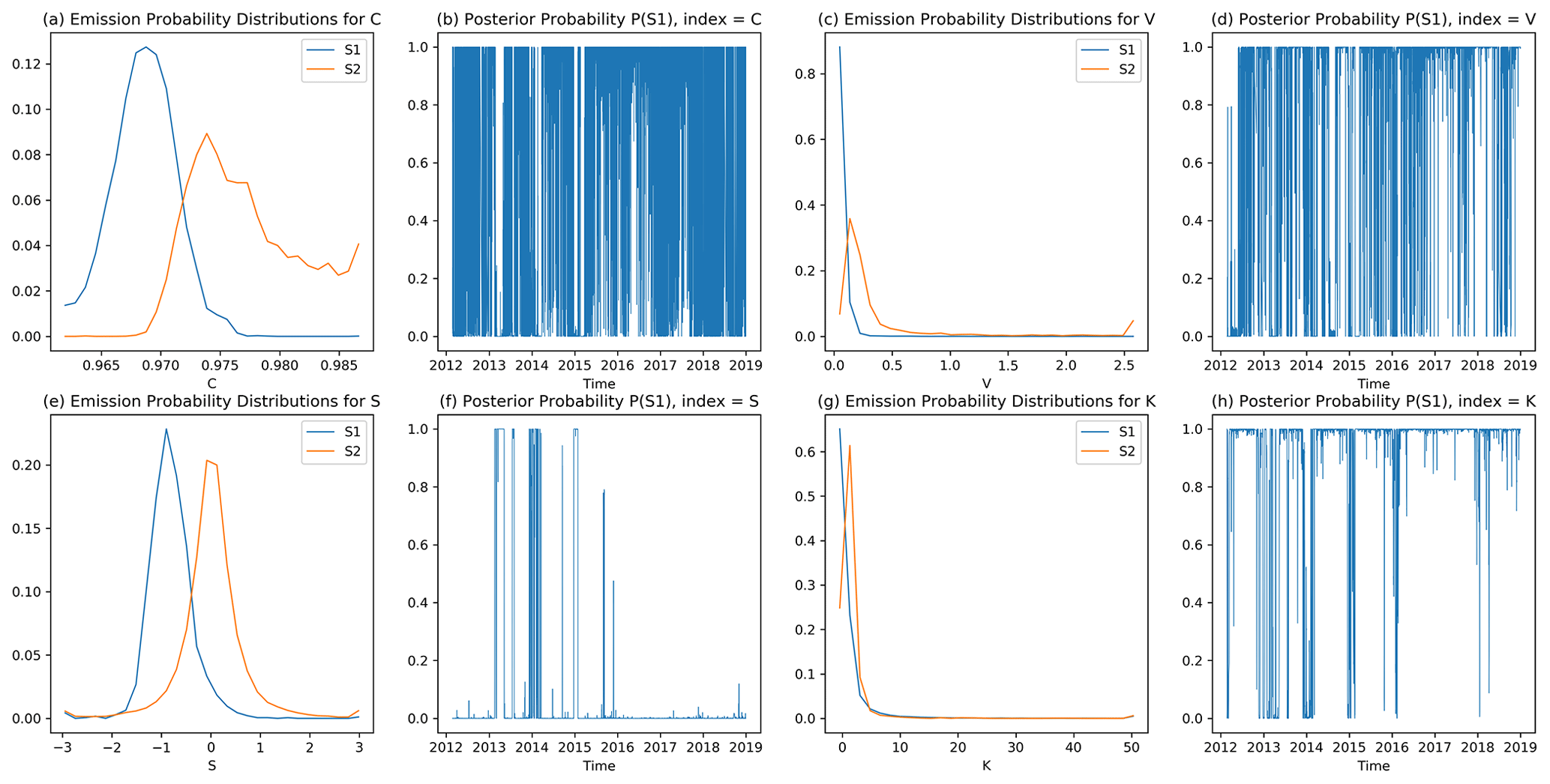
Figure 3 The output of BWA: the emission probability or the probability mass functions, as well as their posterior HS probability TSs, for ${\stackrel{\mathrm{‾}}{\stackrel{\mathrm{‾}}{C}}}_{\mathrm{NS},t}$ (a, b), ${\stackrel{\mathrm{‾}}{\stackrel{\mathrm{‾}}{V}}}_{\mathrm{NS},t}$ (c, d), ${\stackrel{\mathrm{‾}}{\stackrel{\mathrm{‾}}{S}}}_{\mathrm{NS},t}$ (e, f), and ${\stackrel{\mathrm{‾}}{\stackrel{\mathrm{‾}}{K}}}_{\mathrm{NS},t}$ (g, h), using KAOH's geoelectric TS data with 50 bins.

The BWA has no problem dealing with high-dimensional problems, provided the inputs are discrete. However, this method would work well only if the overall number of possible observations is small. If we use 50 bins for each of the eight indexes, there would be $D={\mathrm{50}}^{\mathrm{8}}\approx \mathrm{3.91}\times {\mathrm{10}}^{\mathrm{13}}$ possible observations, meaning the emission matrix would be of dimensions 3.91×10¹³ by 2. Reducing the number of bins to just 10 for each index, we still have D=10⁸ possible observations. This latter space is still too large for the BWA to search through exhaustively in a reasonable amount of time, even though we feel 10 bins for each index may already be too coarse and likely to miss subtle details. Furthermore, with so many possible observations, we expect the emission probabilities to be significantly different from 0 only for a very small subset of the D possible observations.

We do not know a priori what the elements of this very small subset are. They may occur as isolated points in the search space, or they may occur in groups of closely spaced points. In the continuous feature space, each of these groups of observations represents a cluster of similar feature vectors. To determine the number of such clusters and where they occur in the 8-dimensional continuous feature space, we mapped similar feature vectors to the same label using the k-means clustering algorithm (Gupta et al., 2010; Wen et al., 2006; Dash et al., 2011), which is commonly used for discretizing continuous vectors such as F_t. We chose to use the k-means clustering for discretizing F_t because of its low computational cost as well as its reliability in grouping similar feature vectors in the feature space. In so doing, we created a discrete feature space with reasonable size as high-level labels of different geoelectric dynamics. The mathematical details of k-means clustering can be found in Sect. S3.

The indexes C_NS,t, V_NS,t, S_NS,t, and K_NS,t have highly disparate dynamic ranges and should not be directly combined into a feature vector. Therefore, before the clustering, we first standardized our indexes by dividing them by their respective standard deviations. The purpose of this step is to ensure the weights associated with each index during the k-means clustering are equal so as not to bias our search for features with high dynamic range. Mathematically, the feature vector of standardized indexes at time t, ${\mathit{F}}_t^{\prime }$, can be written as

$$\begin{array}{}\text{(5)}& \begin{array}{rl}{\mathit{F}}_t^{\prime }& =\left[{\displaystyle \frac{C_{\mathrm{NS},t}}{\mathit{\sigma }\left(C_{\mathrm{NS},t}\right)}},{\displaystyle \frac{V_{\mathrm{NS},t}}{\mathit{\sigma }\left(V_{\mathrm{NS},t}\right)}},{\displaystyle \frac{S_{\mathrm{NS},t}}{\mathit{\sigma }\left(S_{\mathrm{NS},t}\right)}},{\displaystyle \frac{K_{\mathrm{NS},t}}{\mathit{\sigma }\left(K_{\mathrm{NS},t}\right)}},\right.\\ & \left.{\displaystyle \frac{C_{\mathrm{EW},t}}{\mathit{\sigma }\left(C_{\mathrm{EW},t}\right)}},{\displaystyle \frac{V_{\mathrm{EW},t}}{\mathit{\sigma }\left(V_{\mathrm{EW},t}\right)}},{\displaystyle \frac{S_{\mathrm{EW},t}}{\mathit{\sigma }\left(S_{\mathrm{EW},t}\right)}},{\displaystyle \frac{K_{\mathrm{EW},t}}{\mathit{\sigma }\left(K_{\mathrm{EW},t}\right)}}\right].\end{array}\end{array}$$

We then implemented k-means clustering using the scikit-learn package (v0.23.1) in Python (v3.6.5), on the sequence of feature vectors ${\mathit{F}}_t^{\prime }$ covering the time period from January 2012 to December 2018. The choice of the number of clusters Q was determined as part of the hyperparameter optimization, described in Sect. 3.5. In this way, we matched each ${\mathit{F}}_t^{\prime }$ to a discrete label o_t→O_q (where q is an integer from 1 to Q) to obtain the TS of discrete observations $\left\{o_{\mathrm{1}},o_{\mathrm{2}},\mathrm{\dots },o_t,\mathrm{\dots },o_T\right\}$ for each station as its input to the BWA.

2.5 Implementation of BWA

In this section, we describe how we implemented the BWA to obtain one HS TS for each station. We start by describing how we initialized and iterated the BWA, as well as how we dealt with local optima in the BWA results by using multiple initializations.

The first step of the BWA is to initialize the HMM parameters $\left(\mathbf{A},\mathbf{B},\mathit{\pi }\right)$. Since we had no prior knowledge on the model parameters, we initialized parameters $\left({\mathbf{A}}_{\mathrm{0}},{\mathbf{B}}_{\mathrm{0}},{\mathit{\pi }}_{\mathrm{0}}\right)$ randomly. After this, we iterated BWA's expectation maximization steps 30 times, starting with iteration index i=1. Each iteration comprises the forward procedure, the backward procedure, and the update. In Sect. S4, we present the mathematical details of how the forward procedure, the backward procedure, and the update are performed.

As the iteration goes, the BWA improves the likelihood of observing the input observation TS $o_{\mathrm{1}},o_{\mathrm{2}},\mathrm{\dots },o_T$ given the model parameters $\left({\mathbf{A}}_i,{\mathbf{B}}_i,{\mathit{\pi }}_i\right)$, which converges when the improvements on the posterior probability $P(o_{\mathrm{1}},o_{\mathrm{2}},\mathrm{\dots },o_T\mathrm{|}\left({\mathbf{A}}_i,{\mathbf{B}}_i,{\mathit{\pi }}_i\right))$ become minimal. In practice, we found that 30 iterations were long enough for most models to converge. We therefore obtained the estimated model parameters $\left(\stackrel{\mathrm{̃}}{\mathbf{A}},\stackrel{\mathrm{̃}}{\mathbf{B}},\stackrel{\mathrm{̃}}{\mathit{\pi }}\right)=\left({\mathbf{A}}_{\mathrm{30}},{\mathbf{B}}_{\mathrm{30}},{\mathit{\pi }}_{\mathrm{30}}\right)$, as well as the posterior probability TS of $\mathit{P}(s_t=S_l\mathrm{|}{o}_{\mathrm{1}},o_{\mathrm{2}},\mathrm{\dots },o_T,\stackrel{\mathrm{̃}}{\mathbf{A}},\stackrel{\mathrm{̃}}{\mathbf{B}},\stackrel{\mathrm{̃}}{\mathit{\pi }})$ for both HSs and all t values, which we write in short form as ${\mathit{P}}_{\mathrm{1}}=\left(P\left(s_{\mathrm{1}}=S_{\mathrm{1}}\right),P\left(s_{\mathrm{2}}=S_{\mathrm{1}}\right),\mathrm{\dots },P\left(s_T=S_{\mathrm{1}}\right)\right)$ and ${\mathit{P}}_{\mathrm{2}}=\left(P\left(s_{\mathrm{1}}=S_{\mathrm{2}}\right),P\left(s_{\mathrm{2}}=S_{\mathrm{2}}\right),\mathrm{\dots },P\left(s_T=S_{\mathrm{2}}\right)\right)$. Here, we noted that BWA assigns the indexing of HSs randomly; therefore, the S₁ of one station is not guaranteed to be equivalent to the S₁ of another station.

We cannot simply do the above BWA estimation once to obtain $\left(\stackrel{\mathrm{̃}}{\mathbf{A}},\stackrel{\mathrm{̃}}{\mathbf{B}},\stackrel{\mathrm{̃}}{\mathit{\pi }}\right)$ because the BWA converges to local optima instead of the global optimum in the model parameter space (Bilmes, 1998; Yang et al., 2017; Larue et al., 2011). Also, the initial parameters have a significant influence on the local optimum where the BWA converges. In order to obtain a global optimum result within a reasonable computation time, we ran 15 BWA estimations in parallel for each station, with different random initial parameters. For each station, we then chose the model with the highest model score given by $P\left(o_{\mathrm{1}},o_{\mathrm{2}},\mathrm{\dots },o_T\mathrm{|}\left(\stackrel{\mathrm{̃}}{\mathbf{A}},\stackrel{\mathrm{̃}}{\mathbf{B}},\stackrel{\mathrm{̃}}{\mathit{\pi }}\right)\right)$ for subsequent analysis. Later in Fig. 4a, we also show all 15 HMMs to demonstrate how consistent the converged models are. We can write the posterior probability TS of this model as ${\stackrel{\mathrm{̃}}{\mathit{P}}}_{\mathrm{1}}=(P\left(s_{\mathrm{1}}=S_{\mathrm{1}}\right)$, $P\left(s_{\mathrm{2}}=S_{\mathrm{1}}\right),\mathrm{\dots },P\left(s_T=S_{\mathrm{1}}\right)\mathrm{|}{o}_{\mathrm{1}},o_{\mathrm{2}},\mathrm{\dots },o_T$, $\left(\stackrel{\mathrm{̃}}{\mathbf{A}},\stackrel{\mathrm{̃}}{\mathbf{B}},\stackrel{\mathrm{̃}}{\mathit{\pi }}\right))$.

For each initial condition, the BWA randomly assigns one HS to be S₁ and the other to be S₂. To show all 15 HMMs simultaneously in Fig. 4a, we need to standardize S₁ and S₂ across all HMMs. For this purpose, we set ${\stackrel{\mathrm{̃}}{\mathit{P}}}_{\mathrm{1}}$ as the “standard”. For the remaining 14 posterior probabilities ${\left\{{\mathit{P}}_{\mathrm{1}}^i\right\}}_{i=\mathrm{2},\mathrm{\dots },\mathrm{15}}$, we checked their expected absolute difference, EAD = mean$\left(\mathrm{|}{\stackrel{\mathrm{̃}}{\mathit{P}}}_{\mathrm{1}}-{\mathit{P}}_{\mathrm{1}}^i\mathit{\}}\right)$, from ${\stackrel{\mathrm{̃}}{\mathit{P}}}_{\mathrm{1}}$, whose value ranges from 0 to 1. If EAD > 0.5, ${\mathit{P}}_{\mathrm{1}}^i$ is more similar to ${\stackrel{\mathrm{̃}}{\mathit{P}}}_{\mathrm{2}}$ than to ${\stackrel{\mathrm{̃}}{\mathit{P}}}_{\mathrm{1}}$, and we proceed to swap the HS indexing for the ith HMM by assigning ${\mathit{P}}_{\mathrm{1}}^i\left(\mathrm{new}\right)\equiv {\mathit{P}}_{\mathrm{2}}^i$ and ${\mathit{P}}_{\mathrm{2}}^i\left(\mathrm{new}\right)\equiv {\mathit{P}}_{\mathrm{1}}^i$. Otherwise, ${\mathit{P}}_{\mathrm{1}}^i$ corresponds to the same HS as ${\stackrel{\mathrm{̃}}{\mathit{P}}}_{\mathrm{1}}$, and we leave its HS indexing unchanged. In this way, we standardized all 15 models so that their P₁ can be visualized together in Fig. 4a, with the ${\stackrel{\mathrm{̃}}{\mathit{P}}}_{\mathrm{1}}$ TSs sorted by their model scores $P\left(o_{\mathrm{1}},o_{\mathrm{2}},\mathrm{\dots },o_T\mathrm{|}\left(\stackrel{\mathrm{̃}}{\mathbf{A}},\stackrel{\mathrm{̃}}{\mathbf{B}},\stackrel{\mathrm{̃}}{\mathit{\pi }}\right)\right)$ and the optimal model in the first row. In Fig. 4b, we show the actual posterior probability TS of this optimal model. The figures of 15 HMMs for all 20 stations are included in Sect. S5.

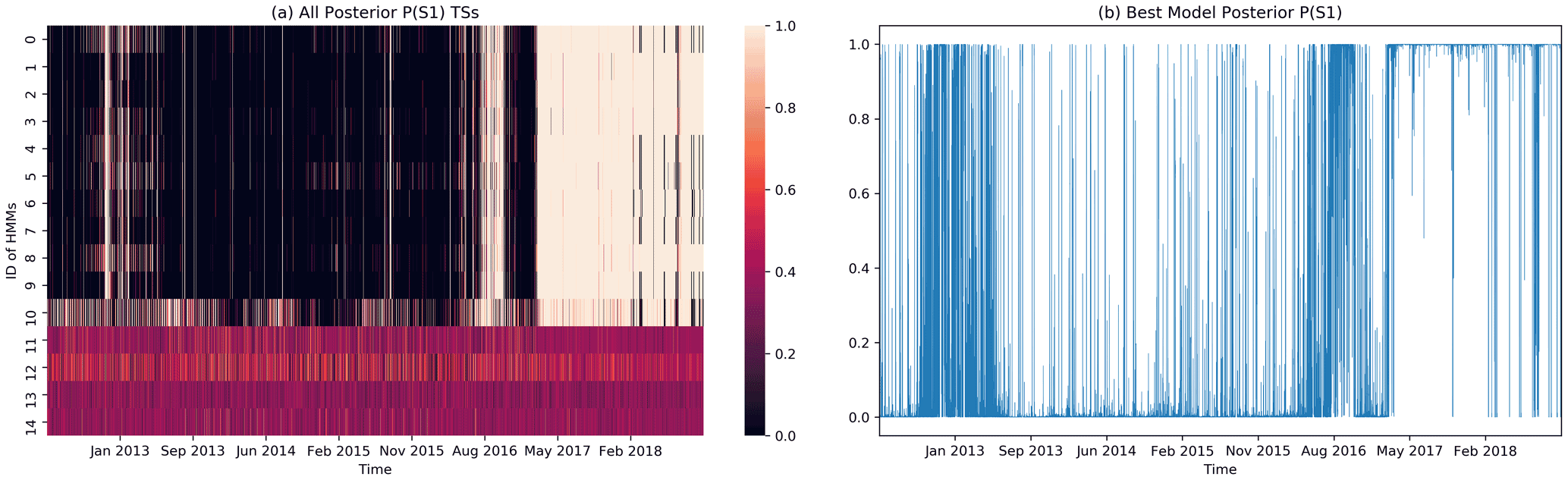
Figure 4 The step-by-step data visualization for CHCH. (a) A heatmap of the 15 HMMs' posterior probability TSs for S₁, sorted by model score from highest to lowest. The posterior probabilities for the last 4 HMMs are messy because the BWA estimations do not converge; (b) the optimal model's posterior HS probability TS for S₁ and ${\stackrel{\mathrm{̃}}{\mathit{P}}}_{\mathrm{1}}$ (obtained using optimal hyperparameters: $\left[L_{\mathrm{w}},Q\right]=\left[\mathrm{0.02}\left(\mathrm{d}\right),\mathrm{30}\right])$.

We summarize the procedures used to obtain ${\stackrel{\mathrm{̃}}{\mathit{P}}}_{\mathrm{1}}$, starting from a pair of geoelectric TSs for each GEMS station in the form of a flowchart in Fig. 5. It is noteworthy that the full procedure contains essentially only two hyperparameters: Q and L_w. The figures shown in the “Results and discussions” section use the optimal hyperparameters, whose identification procedure will be discussed in detail later in Sect. 3.5. Additionally, for each station's optimal HMM, we plotted the distribution of indexes (C, V, S, K) at both HSs in Sect. S6.

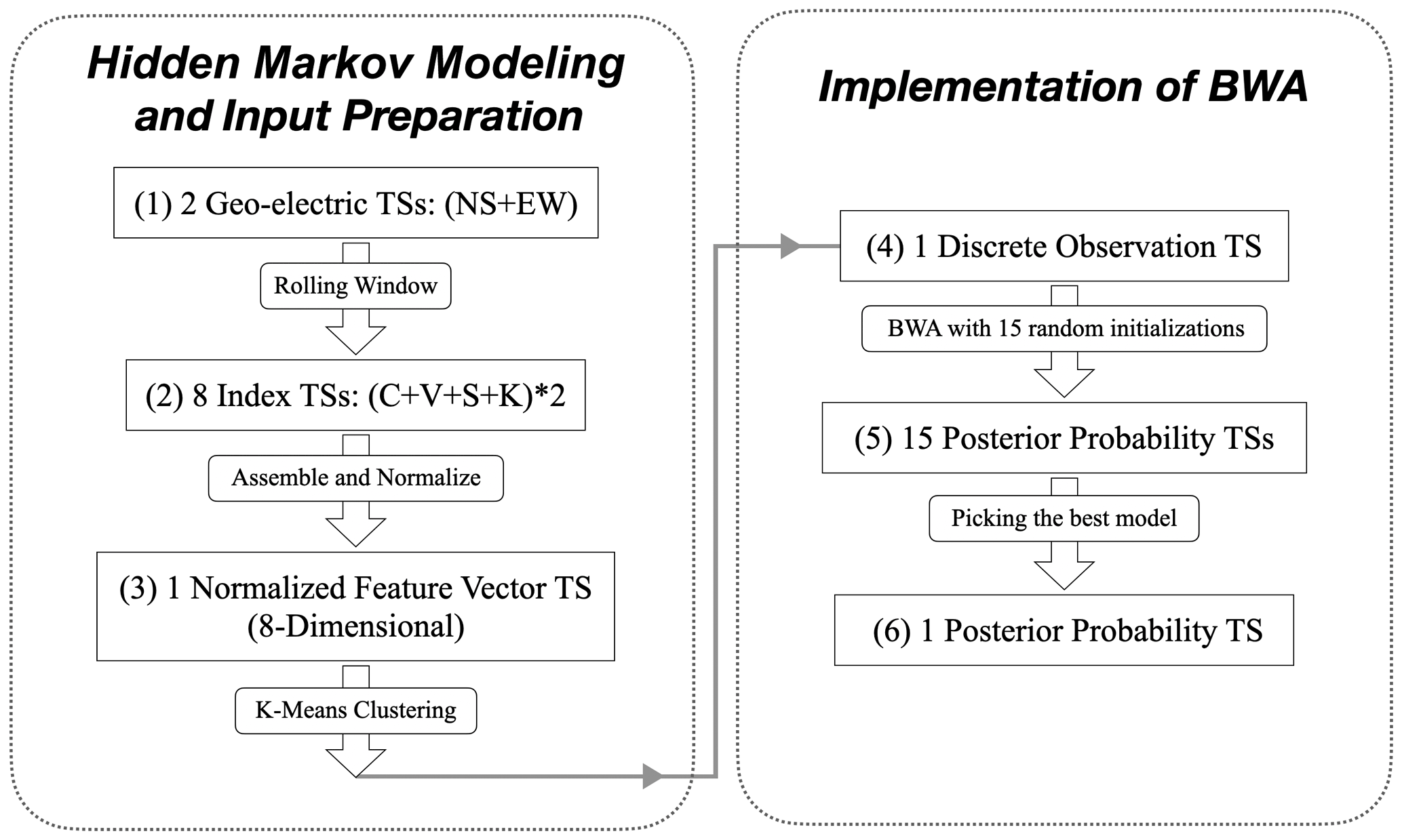
Figure 5 Flowchart summarizing the procedures of obtaining the optimal posterior probability TS ${\stackrel{\mathrm{̃}}{\mathit{P}}}_{\mathrm{1}}$ from the data of one GEMS station.

2.6 EQ grid map, EQ frequency, and EQ frequency ratio

Up to this point, we did not incorporate any EQ catalog information into ${\stackrel{\mathrm{̃}}{\mathit{P}}}_{\mathrm{1}}$ for each station. Unlike many past EQ studies looking for specific precursory features within the geoelectric data, we made no specific assumptions regarding what these EQ precursors might look like. Instead, we let the BWA search for specific precursory features within the 8-dimensional feature space.

After the hidden Markov modeling, we then checked locally whether S₁ and S₂ would effectively partition time periods with significantly lower EQ probabilities from those with significantly higher EQ probabilities. We think of one HS as a passive state (with significantly lower EQ probabilities) and the other HS as an active state (with significantly higher EQ probabilities), but we cannot call the former S₁ and the latter S₂ because we have not yet standardized these HS labels across the 20 stations. To do so, we need to match the HS TS of each station to the EQ catalog to determine the EQ frequencies of S₁ and S₂ for this station and use S₁ and S₂ as the HS labels of the active and passive states respectively (relabeling when necessary). In the remainder of this section, we describe in detail how this is done.

For each GEMS station we started from ${\stackrel{\mathrm{̃}}{\mathit{P}}}_{\mathrm{1}}$ and classified time periods across the 7 years as belonging to two sets T₁ and T₂. The time point t_i was assigned to T₁ if ${\stackrel{\mathrm{̃}}{P}}_{t_i}\left(S_{\mathrm{1}}\right)>\mathrm{0.5}$ and to T₂ if ${\stackrel{\mathrm{̃}}{P}}_{t_i}\left(S_{\mathrm{2}}\right)>\mathrm{0.5}$. After this is done, we checked how EQs are distributed between T₁ and T₂ for different regions across Taiwan. For this task, we first made a 16-by-16 grid map of Taiwan so that EQs within the same grid cell (ix, iy), for ix and iy in $\left\{\mathrm{0},\mathrm{1},\mathrm{\dots },\mathrm{15}\right\}$, are grouped together (see Fig. 6).

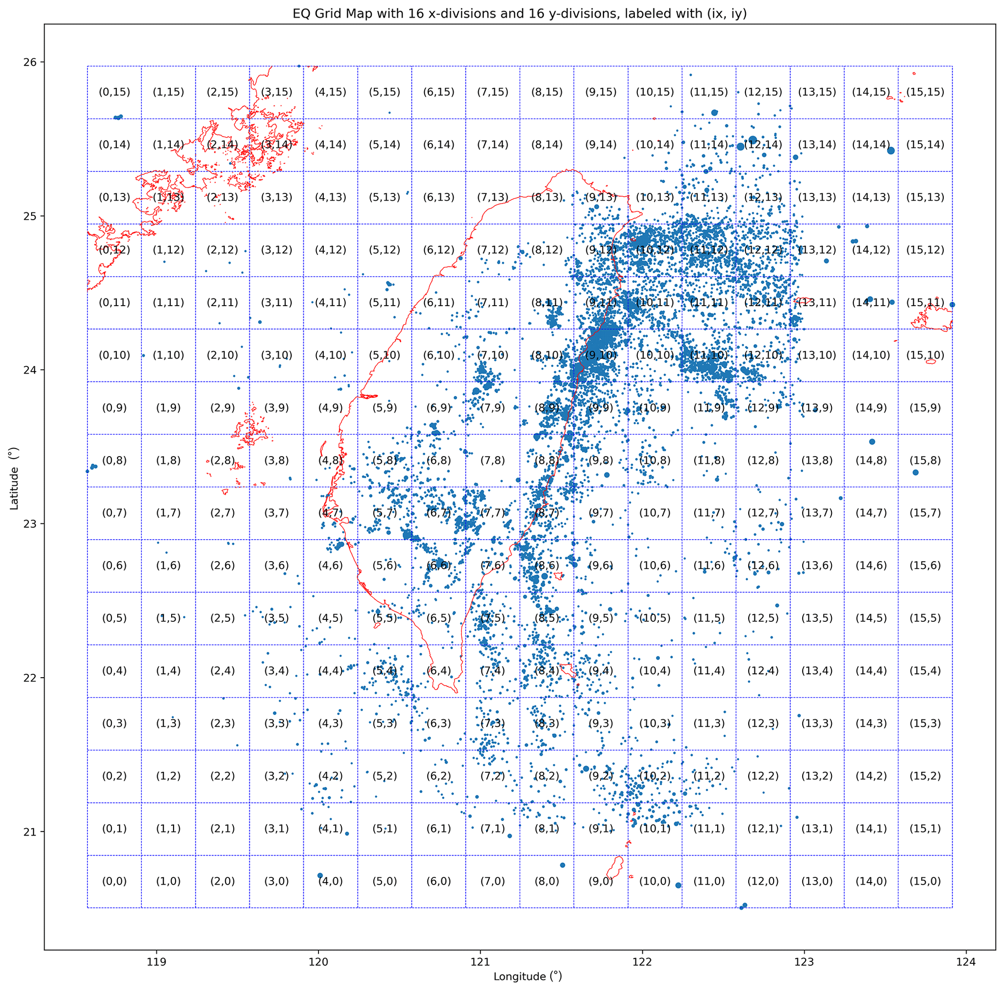
Figure 6 A sample EQ grid map with 16 by 16 divisions, in which each cell measures 0.3330^∘ (longitude) by 0.3418^∘ (latitude). All EQs of M_L≥3 are labeled with blue circles, with the radius of each circle being proportional to the natural exponential of the EQ's magnitude.

For each grid cell (ix, iy), we defined the EQ frequencies for HSs S₁ and S₂ as

$$\begin{array}{}\text{(6)}& F_{\mathrm{EQ},\mathrm{1}}={\displaystyle \frac{N_{\mathrm{1}}}{\left|T_{\mathrm{1}}\right|}},F_{\mathrm{EQ},\mathrm{2}}={\displaystyle \frac{N_{\mathrm{2}}}{\left|T_{\mathrm{2}}\right|}},\end{array}$$

where N₁ is the number of EQs occurring within T₁, N₂ is the number of EQs occurring within T₂, |T₁| is the total duration of T₁ time periods, and |T₂| is the total duration of T₂ time periods. From Fig. 6, we see that the spatial distribution of EQs is highly heterogeneous, so we may find a grid cell with about 10 EQs but also another grid cell with about 1000 EQs. This tells us that we should not directly compare the EQ frequencies but should instead compare the EQ frequency ratio, defined as

$$\begin{array}{}\text{(7)}& R_{\mathrm{F}}={\displaystyle \frac{F_{\mathrm{EQ},\mathrm{1}}}{F_{\mathrm{EQ},\mathrm{1}}+F_{\mathrm{EQ},\mathrm{2}}}}.\end{array}$$

For any cell containing at least one EQ, the range of its R_F is [0,1]. Intuitively, any cell with R_F<0.5 is a region having lower EQ frequency in S₁ compared to S₂; and any cell with R_F>0.5 is a region having a higher EQ frequency in S₁ compared to S₂. For example, for a cell with R_F=0.2, F_EQ,1 is only one-quarter of F_EQ,2. The R_F value quantifies how one HS has a higher or lower EQ frequency than the other. In Sect. 3, we will present how we deep dived into the spatial–temporal correlations between HS TSs (${\stackrel{\mathrm{̃}}{\mathit{P}}}_{\mathrm{1}}$) and EQ activities for all 20 stations, starting from 20 grid maps of R_F values.

3 Results and discussions

In this section, we present the results obtained for all 20 stations, as well as additional treatments that we felt were necessary to investigate whether the HS TSs have significant forecasting power for EQs.

3.1 EQ frequency ratio (R_F) grid maps

Once we obtained the ${\stackrel{\mathrm{̃}}{\mathit{P}}}_{\mathrm{1}}$ TS for each station, the natural first step of our analysis was to examine the R_F values for all cells in the 16-by-16 grid map. We show this procedure for the CHCH station in Fig. 7, where we visualize the grid maps for N₁ and N₂ in Fig. 7a and b respectively to clearly show how many EQs occurred during T₁ and T₂. The resulting R_F grid map is shown in Fig. 7c, where there are cells with values close to 0.5 (white-color cells) and cells with values far from 0.5 (red for close to 0, green for close to 1). White-color cells are regions whose EQ activities are weakly correlated with the HSs since the time periods of S₁ and S₂ are not very different in terms of EQ frequency; whereas red/green cells are regions with significantly lower/higher EQ frequencies in S₁.

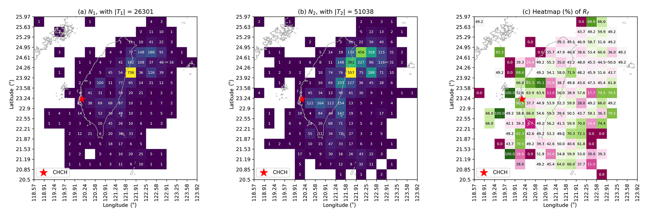
Figure 7 The step-by-step data visualization for CHCH, showing (a) the grid map with the number of M_L≥3 EQs during S₁'s time periods, N₁; (b) the grid map with the number of M_L≥3 EQs during S₂'s time periods, N₂; and (c) the grid map with the EQ frequency ratio, R_F(×0.01). Results were obtained using optimal hyperparameters: $\left[L_{\mathrm{w}},Q\right]=\left[\mathrm{0.02}\left(\mathrm{d}\right),\mathrm{30}\right]$.

As can be seen in Fig. 7c, for different regions the HS with higher EQ activities can be either S₁ or S₂. This is true not only for the CHCH station but also for all 20 stations, whose R_F grid maps are shown in Fig. 8. Although there is no consistent pattern of any state corresponding to higher EQ activities globally, we see in Fig. 8 that there are regions whose R_F values are far from 0.5 across many stations. This means that statistically speaking, one of the HSs has higher EQ activities than the other. In fact, if the active HS has a lot more EQs than the passive HS, it is also likely that the active HS covers most of the larger EQs (e.g., M>5), which is a good attribute for potential EQ forecasting applications. This phenomenon is shown in Sect. S7, where we visualized the EQ frequency distributions across different magnitudes for both HSs for three selected cells with the most EQ events.

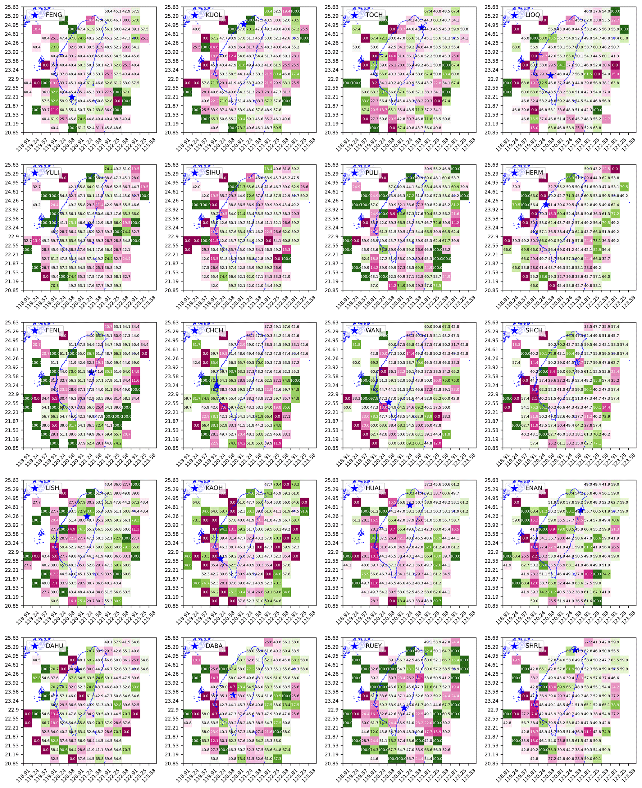
Figure 8 The grid maps of EQ frequency ratio R_F(×0.01) for 20 stations (obtained using optimal hyperparameters individually specified for each station in Fig. 12).

All in all, the findings in this section are important, but we cannot directly decide whether S₁ or S₂ is the proxy for increased EQ probabilities because neither can be associated consistently with the active or the passive state. Instead, we should understand S₁ and S₂ as two high-level, fuzzy labels for tectonic dynamics related to EQ activities in different regions. There can be elements such as rock and soil formations, the underground water system, and fault lines, forming a complex dynamical system that influences where and when EQs become active. Concrete mapping between EQ activities and specific elements of the complex dynamical system would be very difficult, as this would involve high-resolution subterranean surveys. Nevertheless, we can still measure how well S₁ and S₂ can partition the time periods so that one HS can have significantly more EQs than the other. To show this more clearly, we created grid maps of discrimination power D and present them in the next section.

3.2 Discrimination power (D) grid maps

We defined the discrimination power D for each cell as

$$\begin{array}{}\text{(8)}& D=\left|R_{\mathrm{F}}-\mathrm{0.5}\right|.\end{array}$$

The value of D ranges from 0 to 0.5, with 0.5 being the most discriminative since all EQs are found in one HS and 0 being the least discriminative since EQ frequencies are identical between the two HSs. We show the grid maps of D for 20 stations in Fig. 9, which are easier to interpret compared to the grid maps in Fig. 8 where we had to use two different colors. Intuitively, for a region with D=0.25 (not uncommon), one of its HSs would have an EQ frequency 3 times that of the other HS. It can be noted that cells around the edge of the map tend to have very high D values because there are very few EQ events in these cells. This is not a problem as we will take the number of EQs into account later in Sect. 3.3.

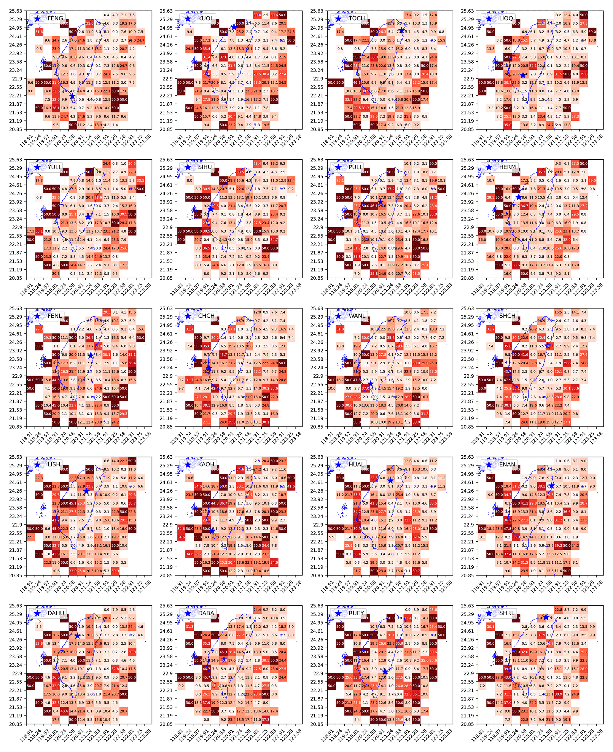
Figure 9 The grid map of discrimination power D(×0.01) for 20 stations (obtained using optimal hyperparameters individually specified for each station in Fig. 12).

In some cells, we find D values close to 0.5, which seems to suggest that the seismicity associated with S₁ is very different from that associated with S₂. However, looking at Fig. 9, we see large variations in D values across the cells and more importantly among some neighboring cells. We therefore wonder whether regions with high D values are statistically significant or the products of random temporal clustering of EQs (Dieterich, 1994; Frohlich, 1987; Holbrook et al., 2006; Batac and Kantz, 2014). For example, if all EQs in a cell occurred within a single day in the 7-year period, any random assignment of HSs would produce the highest D value of 0.5. To address this concern, we investigated the significance of the grid maps of D through statistical tests in the next section.

3.3 Cellular-level significance tests of the forecasting power

Since we had the optimal HMMs for the 20 stations, we can test cellular statistical significance levels indicating that their HSs can indeed separate time periods of higher/lower EQ probabilities, using D grid maps shown in Fig. 9. Specifically, for each grid cell and an empirical HS TS we carried out statistical hypothesis testing using the following null hypothesis: any random HS TS would achieve the same or higher performance (in terms of the D value). To create random HS TSs for the hypothesis testing, we chose to directly simulate the HMM using the same model parameters $\left(\stackrel{\mathrm{̃}}{\mathbf{A}},\stackrel{\mathrm{̃}}{\mathbf{B}},\stackrel{\mathrm{̃}}{\mathit{\pi }}\right)$ as the empirical HMM of the corresponding station. For each hypothesis test of an empirical HS TS (actual HS TS obtained for each station), we created 400 simulated HS TSs, which were then used to create 400 grid maps of the discrimination power D. In Fig. 10, we show the empirical HS TSs alongside a random sample of 10 simulated HS TSs for YULI, SHRL, CHCH, and SIHU to illustrate the simulated counterparts. After this, in each cell, we had one empirical value of D that we can compare against a distribution of 400 simulated values of D. This allows us to compute for each cell the probability that its empirical D value is higher than its simulated counterparts. We named this quantity the discrimination reliability R_D, defined for each cell in the grid map as

$$\begin{array}{}\text{(9)}& R_{\mathrm{D}}={\displaystyle \frac{(\text{no. simulated}D<\text{empirical}D)}{\mathrm{400}}}.\end{array}$$

In the language of statistical hypothesis testing, the p value for the test is given by $p=\mathrm{1}-R_{\mathrm{D}}$. The value of R_D ranges from 0 to 1. If R_D is close to 1, we are confident that the discrimination power of the empirical HS TS is statistically significantly high; otherwise, we have no such confidence.

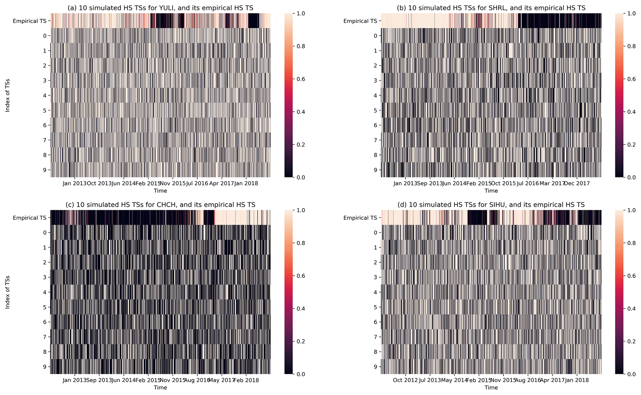
Figure 10 The empirical HS TS and 10 simulated HS TSs, for the stations (a) YULI, (b) SHRL, (c) CHCH, and (d) SIHU. The simulated HS TSs have HS transition frequencies and HS total durations similar to the empirical HS TS but have none of the temporal correlations in the empirical HS TS. Results are obtained using optimal hyperparameters individually specified for each station in Fig. 12.

In Fig. 11, we show the grid maps of R_D values (as percentages) for all 20 stations. Dark-red cells are regions with R_D close to 1, and white and pink cells are regions with R_D close to 0. From these grid maps, we can better appreciate the utility of HS TSs across the grid map since the R_D value is a statistical significance measure of the HS–EQ correlation, unlike the discrimination power D. To explain this, let us take the example of LIOQ (upper left of Fig. 11), whose physical location is marked by the blue star within a dark-red grid cell of R_D=0.992. This means that the empirical HS TS performs better than random guesses (i.e., simulated HS TSs) at separating time periods of low/high EQ frequencies, with a statistical significance of p=0.008. This means that it is improbable for a simulated HS TS to have such a high D, and therefore the empirical HS TS is unlikely to be a product of random chance. This is a very strong demonstration of the mutual information between the HS TS obtained from geoelectric TS and the EQ catalog that was not used to train the HMM.

In the proximity of the LIOQ station located within 22.55–23.58^∘ N, we can see a clear pattern of cells with R_D≥0.9 (dark-red color), while R_D≥0.9 occasionally for most cells outside this general region. This pattern suggests the geoelectric information from LIOQ is approximately local. This is consistent with the logical requirement for a direct/indirect structural relation between LIOQ and region X, such as being close to the same subterranean fault line, for the information at LIOQ to be useful for region X. As a corollary, information given by LIOQ is less likely to be useful for faraway regions as they are less likely to have such structural relations with LIOQ. In application scenarios, this means that the state of EQ probabilities of region X can be estimated using stations closer to the region. Last but not least, it is also worth mentioning that most cells at the edge of the map seldom have high R_D values. This is consistent with the fact that these cells typically have very few EQ events to provide high statistical significance.

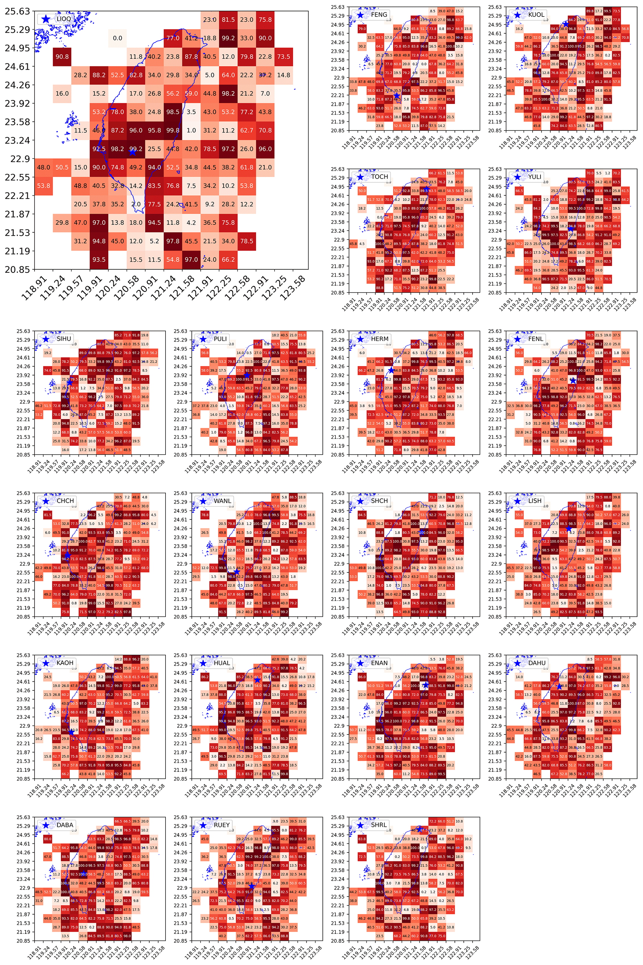
Figure 11 The grid map of discrimination reliability R_D(×0.01) for 20 stations (obtained using optimal hyperparameters individually specified for each station in Fig. 12).

Based on our discoveries regarding the HS–EQ correlations so far, we claim that the HS TSs can provide usable EQ forecasts for real-world applications. We understand that for all EQ forecasting, whether short-, medium-, or long-term, we must specify (a) a time window, (b) a space window, and (c) the magnitudes of EQs expected. We shall next explain how the HS TSs can be useful for EQ forecasting from these three aspects. (a) Let us consider an HMM that started out in the passive state, where EQs of all magnitudes are less frequent compared with the active state. In most stations that we tested, we noticed that once an active state has persisted for a few weeks, it is unlikely to switch back to the passive state until a few months have elapsed. This minimum lifetime found in historical data can be used as a prediction time window. Based on this timescale, we can say that our HMM can be useful for short- to medium-term EQ forecasting, depending on the station of interest. (b) Next, let us consider the grid cells covering Taiwan. For a given grid cell, it may be satisfactory (R_D being high enough) for a list of stations. The more stations in this list becoming persistently active, the more likely large EQs within this grid cell should occur. This is the spatial window we work with for making predictions. (c) Finally, let us describe how our HMM can help in assessing the magnitudes of EQs expected. To answer this question, we can examine the distribution of EQ frequencies across magnitudes 3.0 to 6.0 for both active states and passive states (in Sect. S7). It turns out that for a given grid cell with high R_D, the active state has proportionally more EQs than the passive state across all magnitudes. Therefore, we expect EQs of all magnitudes to be more frequent in a positive prediction.

For grid cells with high R_D, the corresponding HS TS alone is sufficient to make intermediate-term EQ forecasts. However, we also have grid cells where none of the 20 stations provide a sufficiently high R_D value for intermediate-term EQ forecasting on their own. These HS TSs could still be useful if we combine all 20 HS TSs as input features for higher-level forecasting algorithms trained individually for each grid cell. For example, for any region (grid cell), if we want to decide whether it currently belongs to the active regime or the passive regime, an algorithm uses the input from all 20 stations to decide the “local” HS for the given grid cell. This high-level algorithm can for example comprise weight-based model averaging (Marzocchi et al., 2012) or decision trees (Asim et al., 2016). Additionally, the value of R_D can be helpful for the algorithm to decide how to weigh the information given by all 20 stations. For example, we can consider only stations with R_D≥R_{D_min} at the given grid cell. The user-defined threshold R_{D_min} can take on constant values (e.g., 0.9) across the grid map or be location specific, such as being lower (e.g., 0.8) for grid cells where few of the 20 stations have R_D≥0.9. We hope to explore this in future work.

Due to the nature of our HSs, we cannot use them to forecast specific EQs or issue evacuation alarms. What the HSs can do, however, is to provide information with forecasting skill to decision makers, in regions where the HS switched from the passive state to the active state convincingly (i.e., the observed active state is persistent and not a temporary fluctuation), to take courses of action that can lower the potential damage with minimal costs. For example, in the passive state, the building inspection authority can prioritize inspection and the issuing of safety permits to new projects over re-inspections of old buildings. With the arrival of an active state that might last a few months to a few years, local authorities would have the incentive to clear up pending re-inspection works so that fewer old buildings are exposed to potential EQ damage. Other than the re-inspection of old buildings, local authorities could also increase the frequency of safety education and drills to vulnerable groups such as students and construction workers to reduce potential injuries or fatalities due to panic or lack of understanding. Additionally, disaster relief services may use the HS's information to re-deploy the stockpile of relief materials, such as food, clothing, tents, and first-aid kits, whenever necessary. In doing so, the stockpile of relief materials can be brought closer to high-risk regions within a convincing active state to be distributed to victims more cost-effectively after a major EQ.

3.4 Global-level significance tests of the forecasting power

From Fig. 11 alone, we have demonstrated the HS TSs are able to separate time periods of low/high EQ probabilities for regions (cells in the grid map) with high R_D values. While the forecasting power of HS TSs in each of these cells is statistically significant, the more critical among us may wonder whether some of these cells can be significant purely by chance, even though there is in reality no persistent correlation between EQs and HSs. For example, any simulated HS TS in Fig. 10 would have at least a few cells with high R_D values. Therefore, in this next section, we will answer the question of whether these HS TSs indeed contain useful information about EQs or whether the number of “significant” cells can be explained by a random null model where the EQs and HSs are mutually uninformative because we test a large number of cells assuming that they are statistically independent.

In order to answer this question, we need to define a performance metric that can quantify the performance of each station with a single value, instead of a grid map of R_D values. We start by assuming that all stations have zero forecasting skill, but as a result of our statistical test, some cells may still end up with high R_D by chance. A truly informative station should have significantly more cells with high R_D than random guesses. Taking the number of EQs into consideration, we further propose that a truly informative station should have significantly higher EQ counts located in high-performing cells. On the grid map, let us define cells with R_D≥R_{D_min} as satisfactory cells and the rest as unsatisfactory cells, where R_{D_min} is the user-defined threshold that determines how high the R_D should be in order to be considered “high-performing”. As mentioned earlier, it is possible to work out schemes that allow for a regionally acceptable R_{D_min}. Here for simplicity let us consider a scheme with a uniform R_{D_min} across all cells in the grid map. With this setting we can proceed to define the single-value performance metric for each station, as the ratio of EQs in satisfactory cells, or R_EQS, as

$$\begin{array}{}\text{(10)}& R_{\mathrm{EQS}}={\displaystyle \frac{{\sum }_{\mathrm{satisfactory}\mathrm{cells}}{N}_{\mathrm{EQ}}}{{\sum }_{\mathrm{all}\mathrm{cells}}{N}_{\mathrm{EQ}}}},\end{array}$$

where N_EQ is the number of EQs in each cell. This ratio of EQs in satisfactory cells takes on values $\mathrm{0}\le R_{\mathrm{EQS}}\le \mathrm{1}$. Intuitively, if R_EQS=0.4, it means that given the R_{D_min} value, 40 % of all EQs are located within satisfactory cells and are therefore “forecasted” by the station to the level required by the user (i.e., R_{D_min}). Therefore, to show that a station has more forecasting power than random guesses, we proceed to test a given station against the null hypothesis that a random guess (simulated HS TS) can have the same R_EQS as the empirical HS TS or higher.

We carried out this hypothesis test station by station by first computing the R_EQS values of a station's empirical HS TS as well as of 400 HS TSs simulated using the HMM parameters for the given station. We then defined the global confidence level as

$$\begin{array}{}\text{(11)}& \mathrm{GCL}={\displaystyle \frac{(\text{no. simulated}{R}_{\mathrm{EQS}}<\mathrm{empirical}{R}_{\mathrm{EQS}})}{\mathrm{400}}}.\end{array}$$

Similarly to the p value for the cellular-level hypothesis test, the p value for this global-level hypothesis test is given by $p=\mathrm{1}-\mathrm{GCL}$, where the GCL range is [0,1], and gives the probability that the empirical HS TSs have higher R_EQS values than their simulated counterparts. For example, if a station has GCL =0.99, we can say that given the specified R_{D_min}, we are 99 % confident that the empirical HS TS yields a higher R_EQS than its simulated counterparts.

In Fig. 12, we show the results of our global-level significance tests, for a choice of R_{D_min}=0.95, in the form of histograms of the 400 simulated R_EQS values compared against the empirical R_EQS values. Except for the LIOQ and LISH stations, we can see from Fig. 12 that all the other stations have GCL values close to 1. This tells us that the empirical R_EQS values of the 18 stations are statistically significant. We also observed that for R_{D_min}=0.95, the simulated R_EQS values are mostly around (or below) 0.05, meaning that only 5 % of EQs are located in satisfactory cells by chance. In contrast, the empirical R_EQS values are mostly above 0.2, except for TOCH, LIOQ, PULI, HERM, and LISH. These findings suggest the HS TSs' EQ forecasting utility to be significant at the global level.

Last but not least, the histograms for each station in Fig. 12 are created with individually optimized hyperparameters, namely L_w (length of time window to compute indexes C, V, S, and K, in days) and Q (number of clusters for the k-means clustering). The optimal hyperparameter values for each station are indicated in the titles for each station. Let us discuss the details of this optimization process in the next section.

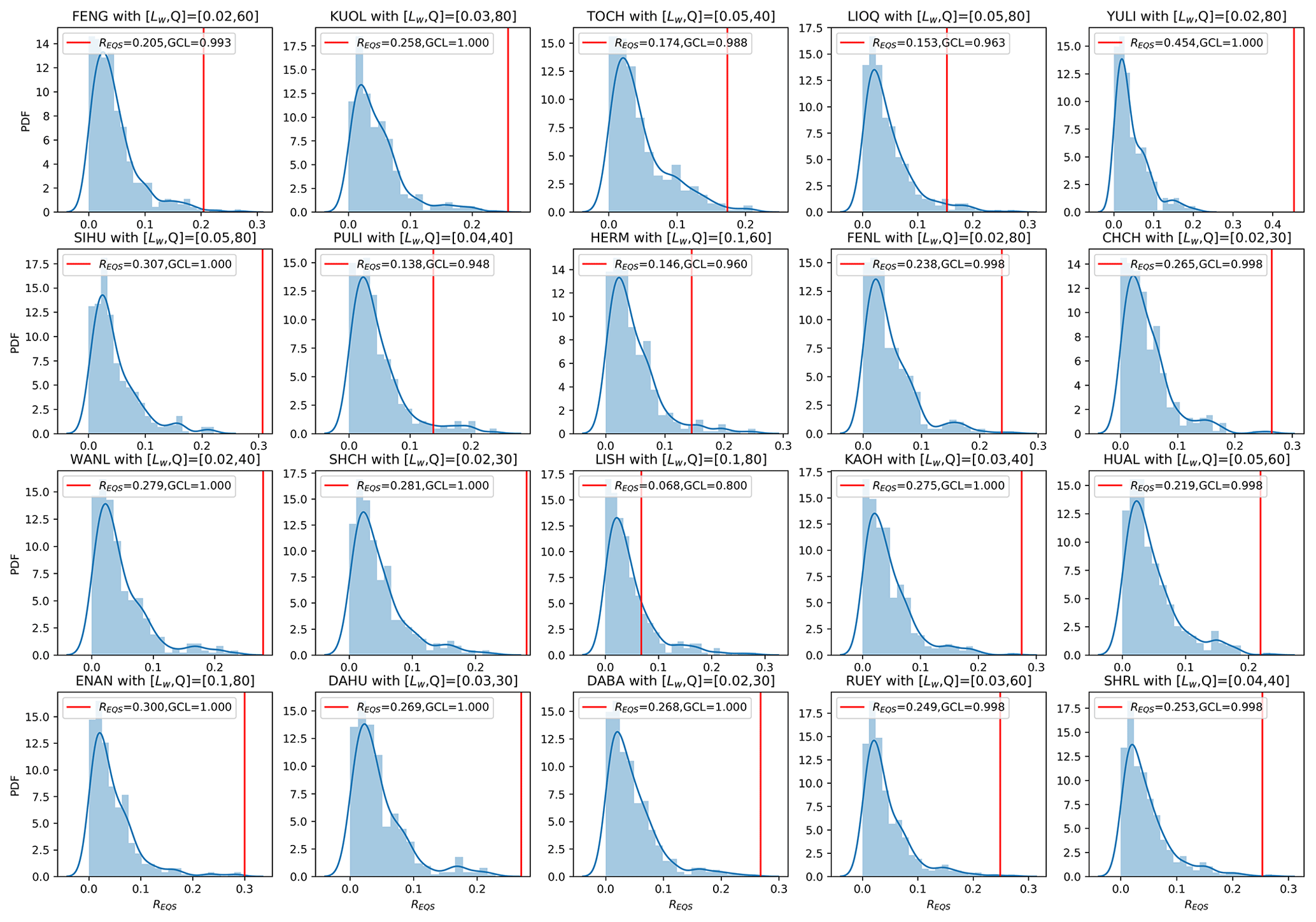
Figure 12 Histograms (blue) of 400 simulated R_EQS values compared against the empirical R_EQS (vertical red line) for 20 stations and R_{D_min}=0.95, with the GCL values in the legends. The hyperparameters of L_w and Q optimized for each station are shown in each subplot's titles.

3.5 Significance levels across the hyperparameter space

Typically, a forecasting model's performance may be sensitive to our choice of hyperparameters. If possible, we would like to choose hyperparameters that make the model the most predictive. If there were too many hyperparameters, this optimization would be challenging in the high-dimensional search space. Fortunately, there are only two hyperparameters needed to obtain the HS TS: L_w and Q. In this section, we show how the model performance (GCL) will vary across the tested hyperparameter space, as well as how we chose the hyperparameters [L_w,Q], for each station. Due to the high computational cost to test each combination of L_w and Q (about 40 min per station on a desktop with 4 GHz quad-core i7 processors, 16 GB of RAM, running macOS Mojave 10.14.6), we performed a coarse grid search over 28 points in the parameter space, consisting of seven different L_w values: $\mathit{\{}\mathrm{0.02},\mathrm{0.03},\mathrm{0.04},\mathrm{0.05},\mathrm{0.1},\mathrm{0.2},\mathrm{0.25}\mathit{\}}$ d (or {28.8, 43.2, 57.6, 72, 144, 288, 360} min) and four different Q values $\mathit{\{}\mathrm{30},\mathrm{40},\mathrm{60},\mathrm{80}\mathit{\}}$. We decided on this search space based on our experience during the model development stage. For real-world applications, where more computational resources can be invested, this hyperparameter optimization can be carried out over a larger and finer grid, in which case better results can be expected.

For each choice of station and hyperparameter, we followed the same procedure of computing 1 + 400 R_EQS values, as well as the resulting GCL value. In Figs. 13 and 14, we show the 20 heatmaps of R_EQS and GCL across the hyperparameter space respectively for R_{D_min}=0.95. The results shown in Fig. 14 are more intuitive, where we found that for many stations, the GCL values approach 1 across broad regions of the hyperparameter space. This can for example be the full hyperparameter space for the YULI station or a patch within the hyperparameter space for the KUOL station. There is just one station (LISH) with poor GCL values everywhere in the hyperparameter space, indicating that there might be exclusive factors that severely limit LISH's forecasting power. For the other 19 stations, the GCL values are close to 1 across either a large area of the parameter space or almost the entire parameter space (e.g., YULI, WANL, ENAN, DABA). This result is compelling and is exactly what we needed for our goal: to demonstrate the forecasting skill of the HS TS, which does not depend on highly optimized hyperparameters but is valid over a broad range of hyperparameters.

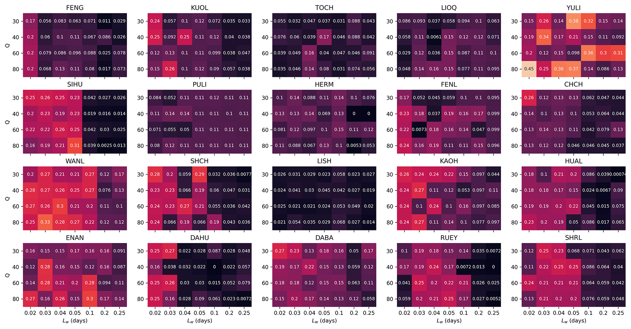
Figure 13 Heatmaps of R_EQS values for all 20 stations across tested hyperparameter space, given R_{D_min}=0.95.

Figure 14 Heatmaps of GCL values for all 20 stations across tested hyperparameter space, given R_{D_min}=0.95.

To wrap up this section, let us describe how to select the optimal hyperparameter for each station. We did this in two steps: first, we selected the hyperparameters with the highest GCL values (1 for many stations); next, in case of ties, we chose the hyperparameter with the highest R_EQS as the winner. For example, for the WANL station in Fig. 14, there are many cells with GCL =1. We therefore proceeded to check the heatmap for WANL in Fig. 13 and identified the hyperparameter combination L_w=0.03 and Q=80 as optimal since it has the highest R_EQS value. Using this selection procedure, we identified the optimal hyperparameter for each station and used these individually optimal hyperparameters to create Figs. 7 to 12. This selection procedure could also be adapted for real-world applications, when more historical data and computational power are available, to provide even better model performances.

4 Conclusions

EQ forecasting is an important research topic because of the potential devastation EQs can cause. As has been pointed out by many past studies, there is a correlation between features within geoelectric TSs and large individual EQs. In those studies, different features of geoelectric TSs were explored for their use of EQ forecasting, among which the GEMSTIP model was the first one to directly use statistic index TSs of geoelectric TSs to produce TIPs for EQ forecasting. Inspired by this, we took a second look at the relationship between these statistic indexes and the timing of EQs and found that there is an abrupt shift in the indexes' distribution along the TTF axis. This suggests that there are at least two distinct geoelectric regimes, which can be modeled and identified using a two-state HMM. This finding is further backed by the knowledge that there can be drastic tectonic configuration changes before and after a large EQ, one important aspect of which being the telluric changes identified in the region around the epicenter of the EQ (Sornette and Sornette, 1990; Tong-En et al., 1999; Orihara et al., 2012; Kinoshita et al., 1989; Nomikos et al., 1997). Therefore, should there be two higher-level tectonic regimes featuring higher/lower EQ frequencies, we would expect to also find two matching geoelectric regimes with contrasting statistical properties, which can be of good utility for EQ forecasting.

Specifically, we modeled the earth crust system as having two HSs identifiable with distinctive geoelectric features encoded by eight index TSs from each station. To obtain the HMM for each station, we needed to run the BWA, which is most convenient to use with a discrete observation TS input. Therefore, we used k-means clustering to convert the continuous TS of 8-dimensional index vectors into a discrete observation TS and subsequently obtained a converged HMM for each station. We then investigated whether these HS TSs provide informative partitions of EQs, i.e., whether one of the HSs can be interpreted as a passive state with less frequent EQs and the other one as an active state with more frequent EQs. For this task, we defined the EQ frequency ratio (R_F), which is the frequency of EQs in one of the HSs divided by the total frequency of the EQs. Using R_F we further defined the discrimination power (D) to measure how different one HS is from the other HS in terms of the EQ frequency. We then plotted 16-by-16 grid maps of R_F and D for all 20 stations and tested the statistical significance of D in each cell by comparing the empirical value against the distribution of D from 400 simulated HS TSs to end up with the grid maps of discrimination reliability (R_D) for all 20 stations. To further investigate the statistical significance level at the global scale, we defined R_EQS to measure the percentage of total EQs located within satisfactory cells, i.e., cells having R_D≥R_{D_min} for a user-specified R_{D_min} value. This R_{D_min} value can be easily customized for different cells, but in this paper, we used a constant R_{D_min} value across the grid map for demonstration. By comparing the R_EQS value of the empirical model against those of 400 simulated models, we obtained one global significance value for each station, namely the global confidence level (GCL). This tells us how confident we can be that information contained in the empirical HS TSs can be used for EQ forecasting.

Finally, we showed how we optimized the GCL values through a grid search in the 2-dimensional hyperparameter space and obtained the optimal combination of L_w and Q individually for each station. As a result, among the 20 stations with optimized hyperparameters, there are 19 stations with GCL > 0.95, 15 of which have GCL > 0.99. Additionally, the confidence levels are also robust across the hyperparameter space for most stations. Based on these positive results, the hidden Markov modeling of the index TSs computed from geoelectric TSs is indeed a viable way to extract information that can be useful for EQ forecasting.

To the best of our knowledge, while there have been previous applications of HMMs for earthquake forecasting, this paper is the first to demonstrate the ability to do so with statistical confidence. As discussed in greater detail in Sect. 3.3, in real-world scenarios, the HS TSs can be useful for intermediate-term EQ forecasting either directly (for high-R_D cells) or as input features for higher-level algorithms that take information from all 20 stations (for low-R_D cells). Beyond our demonstration of extracting EQ-related information from geoelectric TSs, the HMM approach described in this paper can also be explored on other high-frequency geophysical data, such as those from geomagnetic, geochemical, hydrological, and GPS measurements, for EQ forecasting.

At this point, we would like to address the issue of out-of-sample testing (or cross-validation) to support the validity of our model. There are two ways to do this: (1) split a long time series into a training data set to calibrate the model and a testing data set to validate the model and (2) use whatever time series data are available to calibrate the model before collecting more data to validate the model. If the model is statistically stationary (its parameters do not change with time), both approaches are acceptable. However, many would agree that an out-of-sample test with freshly collected data (approach 2) is more impressive, especially if it is performed in real time. We would certainly like to try this and are writing a grant application to fund such a validation study. For this paper, however, we were not even able to use approach 1 because our geoelectric time series are not long enough. This is especially so if we require that (a) the validation data are always temporally after the training data and (b) the validation data are also intermediate term for intermediate-term EQ forecasting. These two requirements cannot be fulfilled using our limited 7-year data if we want to have a significant number of validations (e.g., 10 times) to produce confident claims. Therefore, in this paper, we limited our scope to demonstrating that our model has forecasting skill, without quantifying its exact forecasting accuracy. We argue that we have indeed achieved this, without the use of out-of-sample testing, because in Sect. 3.5, we showed the forecasting skill is statistically significant regardless of the choice of the hyperparameters, for 19 out of the 20 stations that we tested. Furthermore, the statistical hypothesis test has the advantage of giving rigorous p values with moderate computation cost, through simulating the HMM for multiple null-hypothesis tests.