the Creative Commons Attribution 4.0 License.
the Creative Commons Attribution 4.0 License.
 | 17 May 2022
Variable hydrograph inputs for a numerical debris-flow runout model
Andrew Mitchell
Sophia Zubrycky
Scott McDougall
Jordan Aaron
Mylène Jacquemart
Johannes Hübl
Roland Kaitna
Christoph Graf
Debris flows affect people and infrastructure around the world, and as a result, many numerical models and modelling approaches have been developed to simulate their impacts. Observations from instrumented debris-flow channels show that variability in inflow depth, velocity, and discharge in real debris flows is much higher than what is typically used in numerical simulations. However, the effect of this natural variability on numerical model outputs is not well known. In this study, we examine the effects of using complex inflow time series within a single-phase runout model utilizing a Voellmy flow-resistance model. The interactions between model topography and flow resistance were studied first using a simple triangular hydrograph, which showed that simulated discharges change because of local slopes and Voellmy parameters. Next, more complex inflows were tested using time series based on 24 real debris-flow hydrographs initiated from three locations. We described a simple method to scale inflow hydrographs by defining a target event volume and maximum allowable peak discharge. The results showed a large variation in simulated flow depths and velocities arising from the variable inflow. The effects of variable-inflow conditions were demonstrated in simulations of two case histories of real debris flows, where the variation in inflow leads to significant variations in the simulation outputs. The real debris-flow hydrographs were used to provide an indication of the range of impacts that may result from the natural variability in inflow conditions. These results demonstrate that variation in inflow conditions can lead to reasonable estimates of the potential variation in impacts.
- Article
(11234 KB) - Full-text XML
- BibTeX
- EndNote


Debris flows are a common hazard in mountainous terrain. They are characterized by periodic, surging flows of water and debris in channelized paths that can affect people and infrastructure, with disproportionate effects on lower-income countries (Hungr et al., 2014; Dowling and Santi, 2014). The severity and extent of damages from debris flows are largely dependent on flow velocities and depths (Jakob et al., 2012), which are often estimated using numerical runout models. The numerical runout models typically used in engineering applications make significant simplifications of debris-flow physical processes and are generally unable to simulate the complex, surging flow that characterizes debris flows. In this study, we examine how different inflow conditions, generated from real debris-flow hydrographs, affect the modelled debris-flow velocities and flow depths.
Monitoring stations operated in debris-flow channels around the world have collected detailed observations of flow depths, and in some cases surface velocities, using laser scanners, radar measurements, geophones, pressure transducers, and other technologies (Hürlimann et al., 2019). The detailed quantitative data from these instrumented channels confirm eyewitness accounts of debris flows exhibiting surging behaviour, with episodes of greater flow depths, often composed of more debris- and sediment-rich material, separated by lower flow depths composed of more water-rich material. The formation of surges has been attributed to hydraulic roll waves, segregation of coarse material forming wave fronts, or the mobilization of sediment stores (either channel bed or bank failures) (Hübl and Kaitna, 2021, and references therein). Theoretical examinations of the development of surges have included solid–fluid mixture theory, with unsteady, coupled changes in fluid pressures and granular temperatures leading to the unsteady nature of the flow (Iverson, 1997), or variation in the basal resistance and pore pressure, with material segregation resulting in a drained, higher-resistance flow front progressively transitioning to a fully fluid flow (Hungr, 2000). Models employing these theories can reproduce surge formation; however, the simulated flows are not as complex as observed real debris flows.
Some studies have used hydrological methods for estimating debris-flow hydrographs, where a water flow hydrograph is estimated, then bulked with a sediment component (Chen and Chuang, 2014; Gregoretti et al., 2016). However, the intensity and duration of the precipitation may not be the only control on the debris-flow behaviour. Geomorphological boundary conditions, including type, abundance, and production of loose sediment, substantially influence debris-flow initiation (e.g., Bennett et al., 2014). The proportion of the catchment area contributing to a debris-flow event may also vary substantially, from isolated sediment sources subjected to a “fire hose effect”-triggering mechanism (e.g., Berti et al., 2020) to much more diffuse sources leading to debris-flow initiation in only part of a catchment area (Coviello et al., 2021). The coupled hydro-morphodynamic model presented by Kean et al. (2013), which considers interactions between rainfall, sediment characteristics, and channel geometry to reproduce observed surging behaviours of debris flows, is an example of a model that considers these boundary conditions. Despite progress in making detailed observations and modelling debris-flow initiation and surging behaviour, the state of practice for predicting debris-flow hydrographs relevant for engineering hazard assessment still relies heavily on empirical peak discharge estimates (e.g., Rickenmann, 1999).
There are many numerical models in use for estimating debris-flow impacts and intensities, with varying levels of physical complexity and different numerical schemes employed (see McDougall, 2017, for a summary). Extensive work has been done to develop models that explicitly consider the interactions between solids and fluids in a debris-flow event, referred to as a multi-phase flow (Leonardi et al., 2014; Iverson and George, 2014; Mergili et al., 2017; Pudasaini and Mergili, 2019). Although multi-phase flow models are more realistic representations of real debris-flow processes, the level of detail required to define the model inputs limits their application in many information-poor contexts. For this reason, many equivalent-fluid models, where the bulk behaviour of the material is represented by a single, semi-empirical rheology, remain in common use for engineering practice (e.g., McDougall and Hungr, 2004; Christen et al., 2010).
Initial conditions must be specified for both the multi-phase and equivalent-fluid modelling approaches as either a “dam break” or “block” start with a predefined source volume and an initial velocity of zero or an inflow hydrograph at some location along the channel. It can be challenging to assign an initiation location and volume for a block start when performing predictive analysis. Even in the back analysis of debris flows, it can be difficult to determine the initial source location and volume and the amount of path material entrained during an event. The use of equivalent-fluid models with a block start has been criticized for not being in static equilibrium at the beginning of motion (Iverson and George, 2019). However, the assumption of instantaneous strength loss, with the equivalent-fluid parameters representing the liquefied mass, is commonly used to examine the flow-like behaviour of events, acknowledging that the models do not represent the mechanisms of the transition from in-place to flowing material (Aaron et al., 2018).
For practical engineering applications, flow depths and velocities on the debris-flow fan are often what govern debris-flow risk as this is where people and infrastructure tend to be. Thus, using an input hydrograph to simulate the arrival of material on the fan is a potential efficient method to keep the modelling approach relatively simple while better accounting for complex debris-flow behaviour. Hydrograph inputs have been developed for other debris-flow runout models (e.g., Chen and Lee, 2000; Christen et al., 2010; Schraml et al., 2015; Mergili et al., 2017; Deubelbeiss and Graf, 2013); however, selecting an appropriate inflow hydrograph is also a significant challenge, especially considering the variability in natural debris flows highlighted earlier.
The objectives of this paper are to
-
explore how different inflow hydrograph initial conditions affect downstream flow depths and velocities,
-
explore how the flow-resistance model interacts with the inflow conditions, and
-
apply complex inflow conditions to back-analyze two debris-flow case histories.
We describe the methodology for the numerical runout modelling and input hydrograph generation in Sect. 2. We present a parametric analysis with varying flow resistance and inflow conditions using numerical models with a simple geometry (a “numerical flume”) in Sect. 3 and demonstrate the effects of complex hydrographs on simulations of real events in Sect. 4. Sections 5 and 6 include discussions and conclusions, respectively.
To explore the effects of inflow hydrograph shape on simulated runout, we first investigated a simple model and progressively added complexity. In this section, we describe the runout model used, the simple synthetic topography used to test triangular hydrographs, and complex hydrographs derived from records of real events. Finally, we applied the complex hydrographs to cases with natural terrain. This approach allows us to examine the interplay between inflow conditions, flow resistance, and simulation outputs.
2.1 Runout model
In this study, we modified Dan3D, a semi-empirical, depth-averaged, Lagrangian model that simulates landslide motion over 3D terrain (McDougall and Hungr, 2004). Dan3D treats the moving landslide mass as an equivalent fluid whose behaviour is governed by its internal and basal flow resistance (Hungr and McDougall, 2009). The momentum conservation equations are
where ρ is the bulk density; h is the bed-normal thickness; vx and vy are the x and y components of the velocity, where x is in the local direction of motion; gx and gy are the x and y components of gravity; kx and ky are the stress ratios (ratios of horizontal to vertical stresses in the x and y directions); σz is the bed-normal stress; τzx is the basal shear resistance; and E is the entrainment rate (Hungr and McDougall, 2009).
The coordinate system is bed-normal and aligned with the local direction of motion, so the basal resisting stress and entrainment terms only appear in Eq. (1).
Note that throughout this paper, we use the term thickness to refer to the distance in the local bed-normal direction and depth for the vertical distance. The internal rheology is represented by an internal friction angle, which is used to calculate the stress ratios (kx,y) within the moving mass as a function of longitudinal strains (McDougall and Hungr, 2004). The model allows for several possible basal shear resistance relationships to be selected, allowing for changes in material behaviour along the flow path (Hungr and McDougall, 2009). In this study, we use the Voellmy flow-resistance model, which is commonly used by researchers and practitioners to simulate debris-flow motion (see Dash et al., 2021, for a summary of debris-flow case histories calibrated with a Voellmy model).
The Voellmy flow-resistance model is defined as
where f is the Voellmy Coulomb friction parameter, and ξ is the Voellmy velocity-dependent resistance parameter, commonly referred to as the turbulence parameter.
As can be seen in Eq. (3), higher values of ξ lead to lower values of basal shear resistance.
Dan3D uses the smoothed particle hydrodynamics (SPH) numerical technique to discretize the moving mass and allow for behaviours such as flow splitting. SPH is a mesh-free continuum method, which discretizes the moving mass into a set of particles: forces are calculated at the particles, resulting in their displacement, while a free surface is interpolated between the particles to define the stress conditions that give rise to the forces at the particles. Dan3D calculates flow thickness using a Gaussian kernel at each particle, and the free surface at any location is the summation of each kernel's contribution at that location, as shown schematically in Fig. 1 (McDougall and Hungr, 2004).
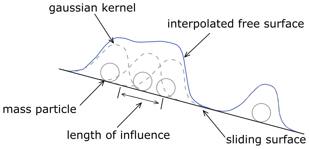
Figure 1Schematic of the SPH technique to interpolate the free surface from the simulation mass particles. The length of influence is three smoothing lengths.
The Dan3D numerical model was originally developed using a block start initial condition, where the debris-flow mass is fully fluidized at the starting time in the model (Hungr and McDougall, 2009). Here, we developed a modified version of Dan3D that allows for fluid particles to be added to the model throughout the simulation so that a wide variety of input hydrographs can be used. The smoothing length calculation that determines the size of the Gaussian kernel (Fig. 1), thus the contribution of each particle to the free surface calculation at a given point, is updated using the dynamic formula outlined by McDougall and Hungr (2004):
where l is the smoothing length, B is the input smoothing length constant, N is the total number of particles, hi is the bed-normal thickness at particle i, and Vi is the volume of particle i.
The modified model calculates an initial value of the smoothing length at time zero based on the initial particle(s) in the model. The number of initial particles depends on the input hydrograph (discussed in Sect. 2.5). The smoothing length calculation can become unstable early in the simulation, and if the value becomes more than 10 times the initial value, the model resets the smoothing length to the initial value. We chose a limit of 10 based on initial testing that showed this value would prevent the smoothing length from approaching infinity early in the simulation while not interfering with the normal fluctuations in Eq. (4). Initial testing shows that the smoothing length calculation generally stabilizes within 20 s (model time) of the simulation start.
The original version of Dan3D utilized multiple flow-resistance models, which can be assigned to areas within the model domain (e.g., allowing for different flow-resistance behaviours in the source area and the deposition area). For this study, we have modified the model to allow for the particles to have different flow-resistance behaviours (i.e., the flow resistance is associated with the particle, not the location).
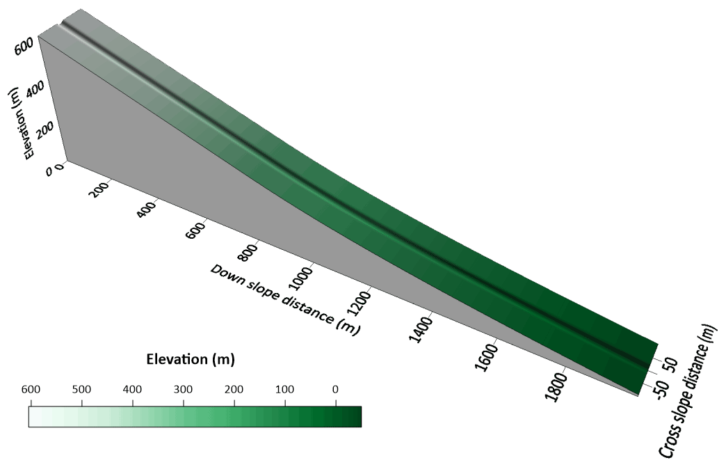
2.2 Numerical flume
We developed an idealized model terrain to conduct numerical experiments on the effects of varying inflow conditions and flow-resistance parameters on the discharge, flow depth, and flow velocity downstream. This numerical flume has a longitudinal profile with a constant 40 % slope (22∘) for the first 780 m and then gradually transitions to a 17 % slope (10∘) over the remaining 1220 m (Fig. 2). The cross section of the model geometry used a smooth curve to define a 10 m deep channel that is 40 m across at the crest with a grid spacing of 3 m. The slopes and channel dimensions for the curved portion of the numerical flume are within the range observed in the upper fans of large debris-flow catchments in southwestern BC (Zubrycky et al., 2021a).
2.3 Triangular inflow hydrographs
We used two approaches to generate the inflow hydrographs: an idealized triangular input and scaled hydrographs observed in the field. A triangular hydrograph is described by the peak discharge (Qp), the total inflow duration (tin), and the time to peak (tp), with the total volume (V) defined by the area of that triangle. Several empirical equations exist for estimating the peak discharge of a debris flow (see Rickenmann, 1999, for a summary), and in this study we utilize the equation based on Froude similarity from Rickenmann (1999):
where c is a constant that ranges between 0.001 and 1, with values of 0.01 typical of muddy flows and 0.1 typical of granular flows (Ikeda et al., 2019). This equation generally agrees with other empirical relationships fit through purely statistical methods (e.g., Mizuyama et al., 1992; Bovis and Jakob, 1999).
With the volume and peak discharge, one can calculate the total inflow duration, but the time to peak must be selected. A recent study of debris flows in the Moscardo catchment in Italy from 2002 to 2019 showed a typical surge duration to be approximately 6 times the time from debris-flow initiation to the peak discharge (Marchi et al., 2021). In this study, the time to peak for the triangular hydrographs is taken as 20 % of the total inflow duration, similar to the general shape found by Marchi et al. (2021) and Hübl and Kaitna (2021).
For this study, we used a triangular hydrograph with a total volume of 100 000 m3 and a peak discharge of 1000 m3 s−1. This volume is within the range of relatively large natural debris flows in the southwestern BC area (Zubrycky et al., 2021a) and well within the range of events used to calibrate the empirical relationships from Rickenmann (1999). The peak discharge corresponds to a value of c=0.07 in Eq. (5), which is near the typical value for a stony debris flow of 0.1 reported by Ikeda et al. (2019). We conducted a parametric study by systematically varying the Voellmy parameters, f between 0.1 and 0.4 and ξ between 25 and 500 m s−2; extracting flow depths and velocities; and calculating the discharge at 1 s increments along cross sections distributed down the model slope. We input all particles at x=300 m, and tested the sensitivity to the inflow location by varying the input distance between x=300 and x=750 m. We also tested the effects of changing the inflow hydrograph by generating a triangular hydrograph with a peak discharge of 2940 m3 s−1 corresponding to a c=0.2 in Eq. (5) for the same volume of 100 000 m3. The c value we selected is an upper envelope from the real-event hydrographs compiled in this study (Sect. 3). We calculated Froude numbers and for both peak discharge cases and compared them to reported values for debris flows.
The effects of modelling a surge consisting of particles with basal resistance defined by two Voellmy materials were also examined. A triangular inflow hydrograph (Qp=1000 m3 s−1) was used as the basis for the two material simulations, with a higher f parameter on the rising limb than the falling limb of the hydrograph. This is meant as a simplified test of the idea of contrasting flow-resistance behaviours resulting in debris-flow surges proposed by Hungr (2000).
2.4 Scaled, real hydrographs
We assembled a dataset of real debris-flow events with high temporal resolution of velocity measurements coupled with flow depth measurements, allowing us to estimate discharge over time. We used these events as prototypes for the modelled inflow into the numerical flume by scaling the discharge. The three sites are Lattenbach, Austria; Dorfbach, Switzerland; and Spreitgraben, Switzerland. They are described in detail in Sect. 3. We kept the inflow duration constant and multiplied the instantaneous discharge by a scaling factor at each time step to obtain a target total volume. We used Eq. (5) to validate that the scaled peak discharge was within a reasonable range for the event volume with an assumed value of the constant c. If the scaled Qp value was unreasonable, we increased the inflow duration to maintain the Qp value within the target range.
As with the triangular hydrographs, we calculated Froude numbers and compared them to literature values for debris flows after applying the scaling. We calculated the intensity index, IDF=dv2, where d is the flow depth, and v is the depth-averaged velocity (Jakob et al., 2012), at various locations along the model channel. The intensity index is commonly used in hazard assessments to calculate building damage from debris flows.
Finally, we tested the sensitivity of simulated impact areas and flow intensities to varying inflow conditions for real, complex topography. The two examples modelled, Mount Currie and Neff Creek, are from southwestern BC, where mapped deposits and field observations provide estimates of flow depths and velocities that were compared to the simulation results. Both sites have at least partial airborne lidar coverage before and after the events for estimates of the deposited volume. We assumed a bulk density of 2000 kg m−3 for the deposited material and a solids density of 2600 kg m−3. We assumed the material in the deposit had a greater density than the flowing material due to drainage and consolidation of the deposited material over time. For the simulations, we assumed the flowing material was fully saturated with a solids content of 50 % by volume, resulting in a bulk density with flowing of 1800 kg m−3, or a total volume considering bulking and water content approximately 1.5 times greater than the deposit volume. For all cases, the model topography consisted of a 3 m DEM of pre-event conditions. We modelled each event using the 24 real input hydrographs scaled to the observed event volume and selected Voellmy parameters based on calibrations not considering variable inflows. To better represent the inferred deposition between stages of the second event (Neff Creek), we implemented a method to represent deposition during flow. We used a Monte Carlo approach that randomly divided the total event volume into four stages and randomly selected an input hydrograph for each of those stages. After each stage, we reduced the final deposit grid by a factor of 0.65 to account for drainage and consolidation (consistent with the assumptions for bulking for the simulation volume estimates) and merged it with the topography grid.
2.5 Hydrograph discretization
We numerically integrated the instantaneous discharge hydrographs for both the triangular and real hydrographs to create a time series of cumulative volume versus time. We then divided the time series by the total event volume to create unit hydrographs and scaled the unit hydrographs to achieve the desired inflow volume. We completed the scaling by multiplying the target volume by the unit hydrograph (assuming the inflow duration is fixed) or by adjusting the inflow time to result in a peak discharge corresponding to a target c value in Eq. (5).
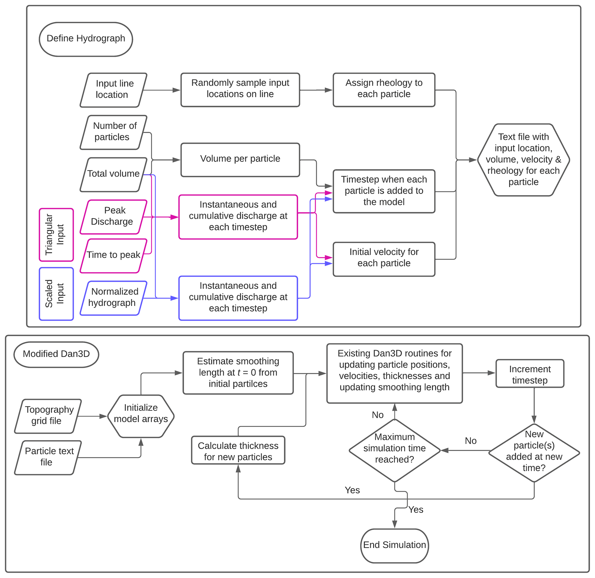
Figure 3Workflow for Dan3D with a hydrograph input. The magenta outlines indicate steps specific to a triangular hydrograph input, while the blue outlines indicate steps specific to a scaled, real hydrograph input.
We generated a cumulative inflow curve from the scaled hydrograph and discretized it into the SPH particles for the simulation. We used a total of 4000 particles in all simulations, with the total volume divided equally between the particles. The particles entered the model domain at a defined inflow line with initial particle positions sampled randomly along that line. We estimated the starting velocities, v, using the following equation (from Rickenmann, 1999):
where S is the channel slope.
We have summarized the runout modelling process as a flow chart in Fig. 3. The “Define Hydrograph” workflow is implemented in R, and the “Modified Dan3D” workflow is implemented in C. We present a visualization of the hydrograph discretization process in Fig. A1 in the Appendix.
The real debris-flow hydrographs are from three sites: Lattenbach, in western Austria, and Dorfbach and Spreitgraben, both in Switzerland. Lattenbach drains an area of approximately 5 km2 and flows through the community of Grins before joining the Sanna River at the community of Pians. The watershed is characterized by deep-seated landslides in weak metamorphic rocks, such as phyllites, and more competent limestone (Hübl and Kaitna, 2021). Dorfbach is in southern Switzerland, where it drains an area of approximately 6 km2 and contains a fast-moving rock glacier as the primary debris source (Jacquemart et al., 2017). There is significant infrastructure near the Dorfbach site, including a road, railway line, and several houses (Deubelbeiss and Graf, 2013). Spreitgraben is in central Switzerland with a catchment area of approximately 4 km2. The debris-flow channel follows an avalanche path, with debris sourced from talus slopes and recent rockfall deposits within the catchment. There is significant infrastructure near the Spreitgraben site, including a road, natural gas pipeline, and several houses (Jacquemart et al., 2015).
Table 1Summary of hydrographs from monitored catchments at Lattenbach (Hübl and Kaitna, 2021) and Dorfbach and Spreitgraben (Jacquemart et al., 2017).
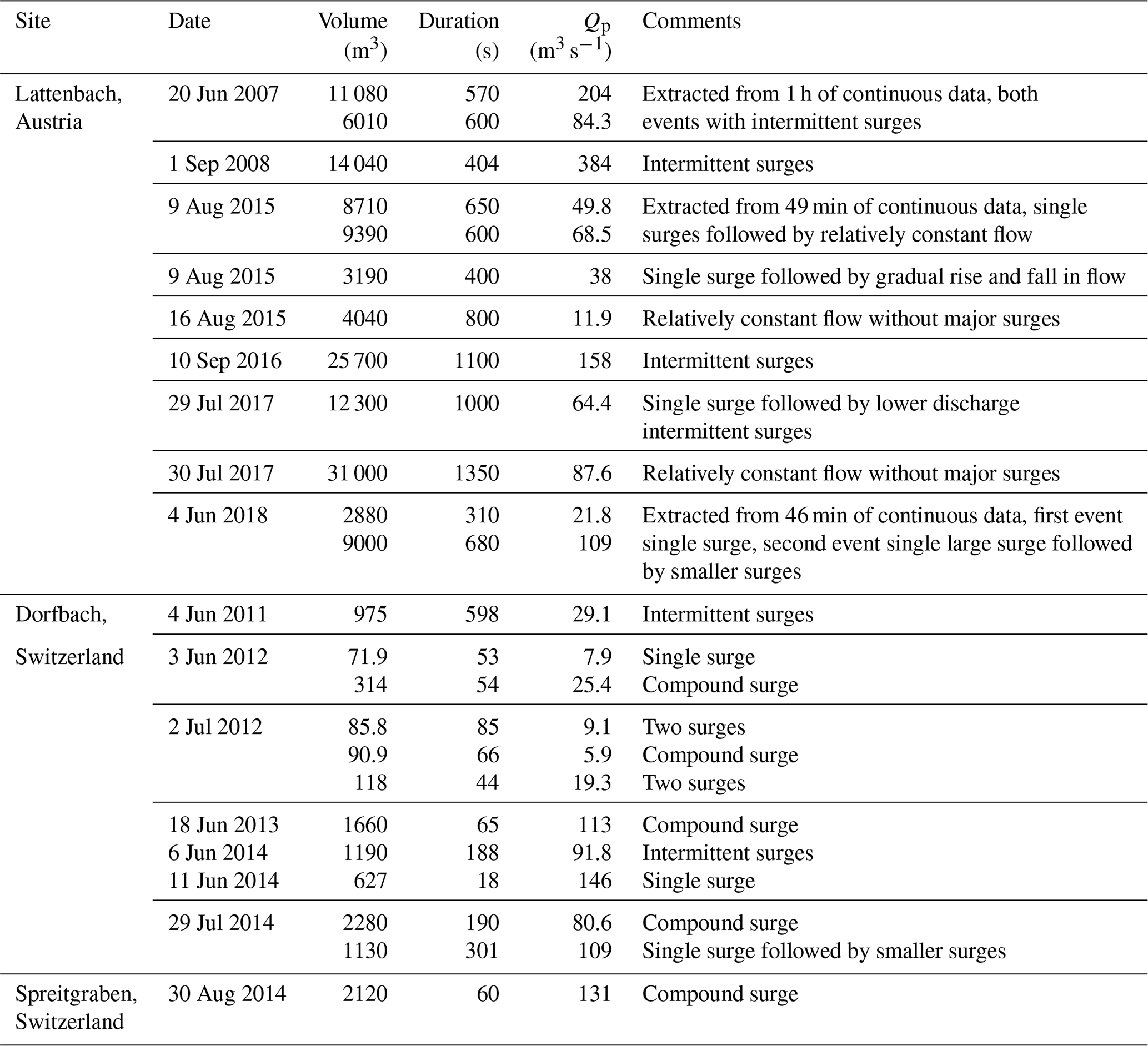
There are records of nine debris flows at Lattenbach between 2007 and 2018 (Arai et al., 2013; Hübl and Kaitna, 2021). The 2007 event records are from Pians, and all others are from higher in the channel at Grins. Three of the debris-flow records were split in two to remove periods with extended low flow between high-flow periods (low-flow periods ranging from 410 and 540 s). There are 11 debris-flow records at Dorfbach between 2011 and 2014 and 1 event record at Spreitgraben in 2014 (Jacquemart et al., 2017). The 24 hydrographs used in this study, including the three split records, are summarized in Table 1. We provided a simple classification of the surge behaviour of each debris-flow observation as either (1) a single surge, most similar to an idealized triangular hydrograph; (2) a compound surge, where there are multiple peaks; or (3) intermittent surges, with distinct surges separated by periods of much lower flow (Hübl, 2021).
The volumes and peak discharges for the 24 cases used in this study are shown in Fig. 4. We selected a c value of 0.2 in Eq. (5) as an upper bound for a plausible peak discharge for the real hydrographs, as shown by the dashed line in Fig. 4.
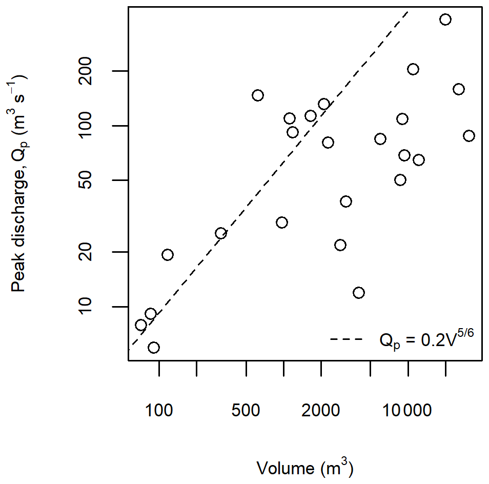
Figure 4Peak discharge versus volume for the cases summarized in Table 2, with the dashed line indicating the values for Eq. (5) with c=0.2.
4.1 Triangular hydrographs
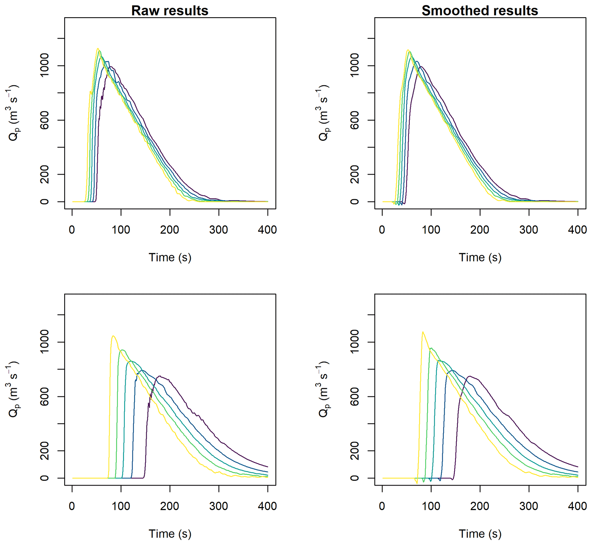
Hypothetical triangular inflow hydrographs were developed following the procedure outlined in Sect. 2.3. Discharge and peak discharge were calculated for all combinations of flow-resistance parameters (Sect. 2.3). Selected discharge results and peak discharge for all cases are shown in Fig. 5. Note that we smoothed the results with a loess function using a span of 15 s to remove small variations in the data due to numerical noise. We provide an example of the difference between the smoothed and raw model results in the Appendix (Fig. A2). In general, the results presented in Fig. 4 show that increasing f reduces the peak discharge, and increasing ξ increases the peak discharge. The modelled peak discharge had little sensitivity to the f or ξ parameters when the f value was significantly less than the model slope, shown by the relatively low variation in peak discharge in Fig. 5a, b, and d versus Fig. 5e.
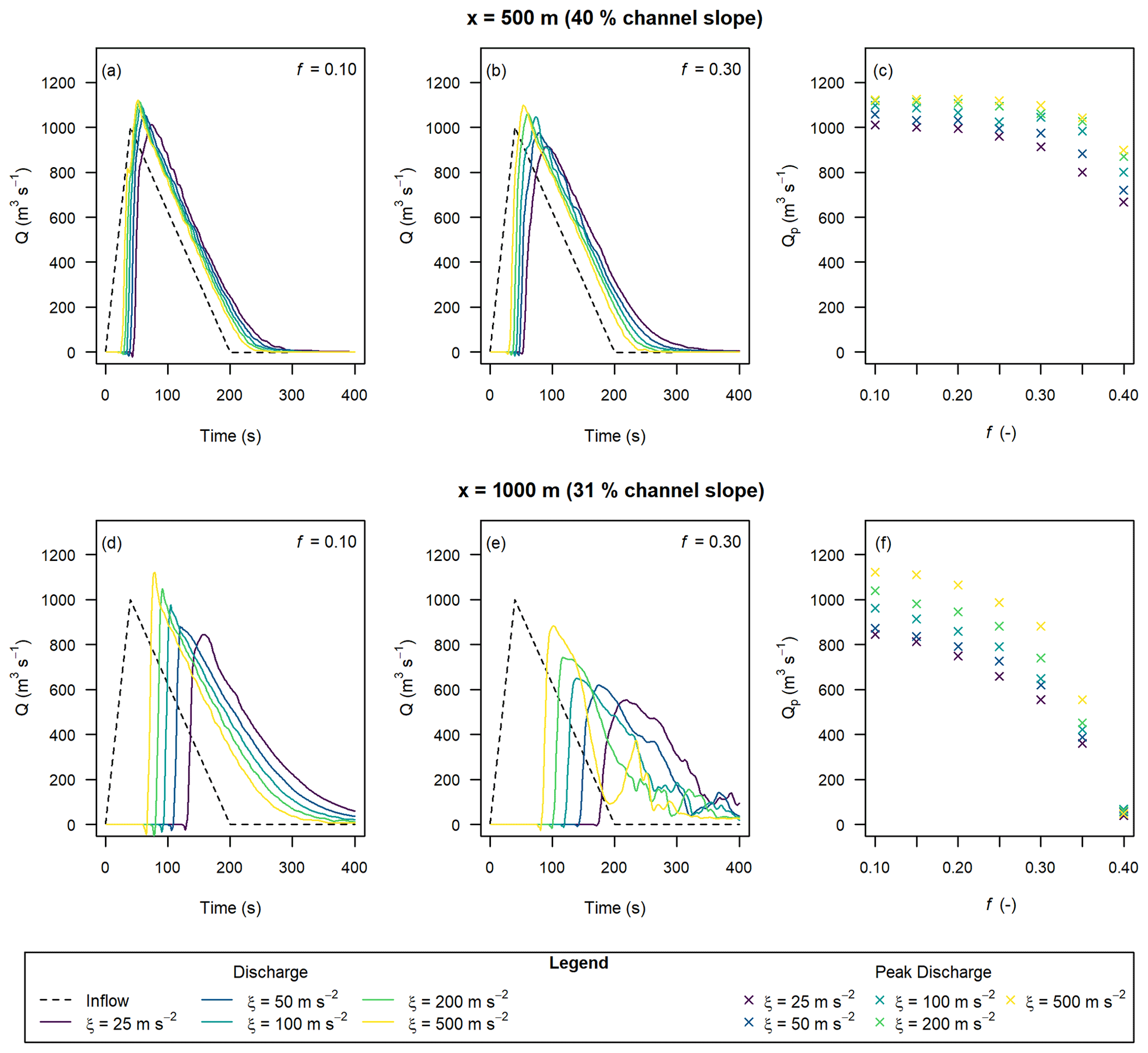
Figure 5Hydrographs extracted at x=500 m (a–c) and x=1000 m (d–f) with varying Voellmy parameters and Qp=1000 m3 s−1, based on triangular input hydrographs.
We also tested the sensitivity of the extracted discharge to the inflow location, as shown in the Appendix (Fig. A3). The inflow location has little effect on the discharge at x=1000 m, except when the friction parameter f is greater than or approximately equal to the local slope at the measurement location. We tested the sensitivity of the extracted discharge to the initial velocity to see if the choice of Eq. (6) to estimate initial velocities had a significant effect on the results (also included Fig. A4 in the Appendix). We found low sensitivity to the input velocity, implying that the Voellmy parameters quickly regulate the simulated discharge. The remaining analyses shown for the numerical flume all used the x=300 m inflow location and Eq. (6) for the initial velocity for consistency.
The sensitivity of the discharge to the Voellmy parameters for the higher-inflow Qp was consistent with the results for the lower-inflow Qp discussed in the previous paragraph. However, the sensitivity to ξ was more prominent, with lower values leading to a more attenuated peak discharge (Fig. 6).
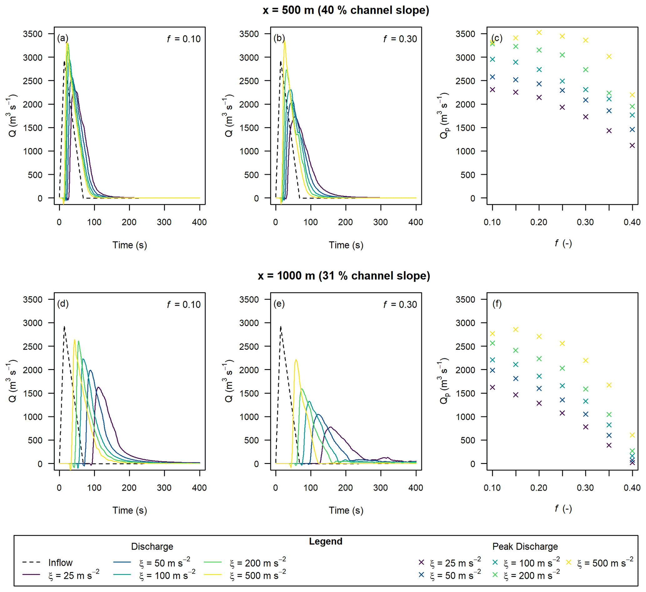
Figure 6Hydrographs extracted at x=500 m (a–c) and x=1000 m (d–f) with varying Voellmy parameters and Qp=2940 m3 s−1, based on triangular input hydrographs.
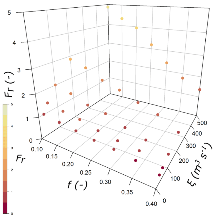
We calculated Froude numbers at the time of peak discharge at x=1000 m to compare with literature values. For the inflow Qp=1000 m3 s−1 cases, the calculated Froude values ranged from 0.32 to 4.06. Froude values ranged from 0.32 to 4.87 for the Qp=2940 m3 s−1 case (Fig. A5), with the higher values corresponding to lower flow-resistance parameters for both peak discharge scenarios. These Froude numbers are within the range of values reported for natural debris flows of 0.45 to 7.6 (Zhou et al., 2019).
By modelling a surge consisting of particles with basal resistance defined by two Voellmy materials, we found the results were most sensitive to the contrast between the ξ1 and ξ2 parameters (Fig. 7). The peak discharge was amplified when the resistance parameters were higher on the rising leg (higher f1, lower ξ1) relative to the inflow hydrograph and relative to the single flow-resistance cases (Fig. 5). This was a result of the lower resistance material on the falling leg pushing against the higher-resistance front. This amplification was most pronounced when the channel slope is steepest, and the peak rapidly attenuates as the channel flattens. The peak discharge is comparable to the peak discharge for the single material simulations when ξ1 is equal to ξ2.
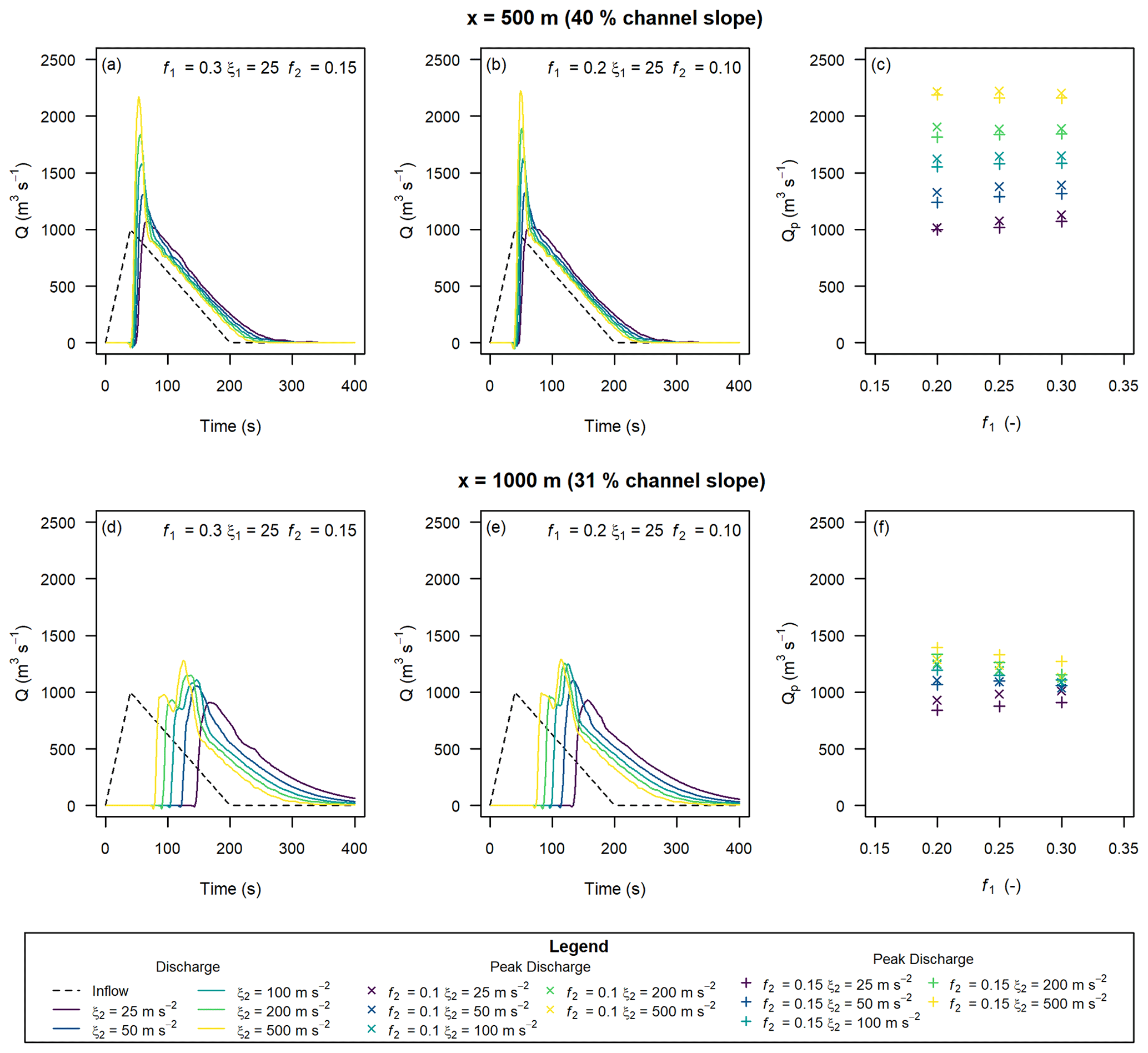
Figure 7Effects of having two sets of Voellmy parameters (f1 and ξ1 on the rising limb and f2 and ξ2 on the falling limb of the inflow hydrograph) on the downstream discharge.
4.2 Scaled, real hydrographs
We ran the models using the 24 debris-flow hydrographs summarized in Table 1, scaled to have a total volume of 100 000 m3 and a maximum Qp of 2940 m3 s−1. Figure 8 compares the extracted hydrographs at x=1000 m with f=0.2 and ξ=200 m s−2 for the Lattenbach inflow hydrographs. Figure 9 compares the extracted hydrographs with the Dorfbach and Spreitgraben inflow hydrographs. We selected these flow-resistance parameters because they did not result in attenuation of the triangular inflow hydrograph between Qp=1000 and 2940 m s−2 at the x=1000 m location (Figs. 5 and 6). There was some attenuation of the largest peak discharges, with the attenuation suspected to be related to the limit of precision in discretizing sharp peaks in the inflow hydrographs into particles and the tendency for the model to attenuate sharper peak discharges (e.g., the greater attenuation in the peak discharges shown in Fig. 6 versus Fig. 5). The Froude number for each case at the peak discharge ranged between 1.64 and 2.37 for the scaled, real hydrographs, which is within the expected range for a debris flow and what was found for the triangular hydrograph inputs.
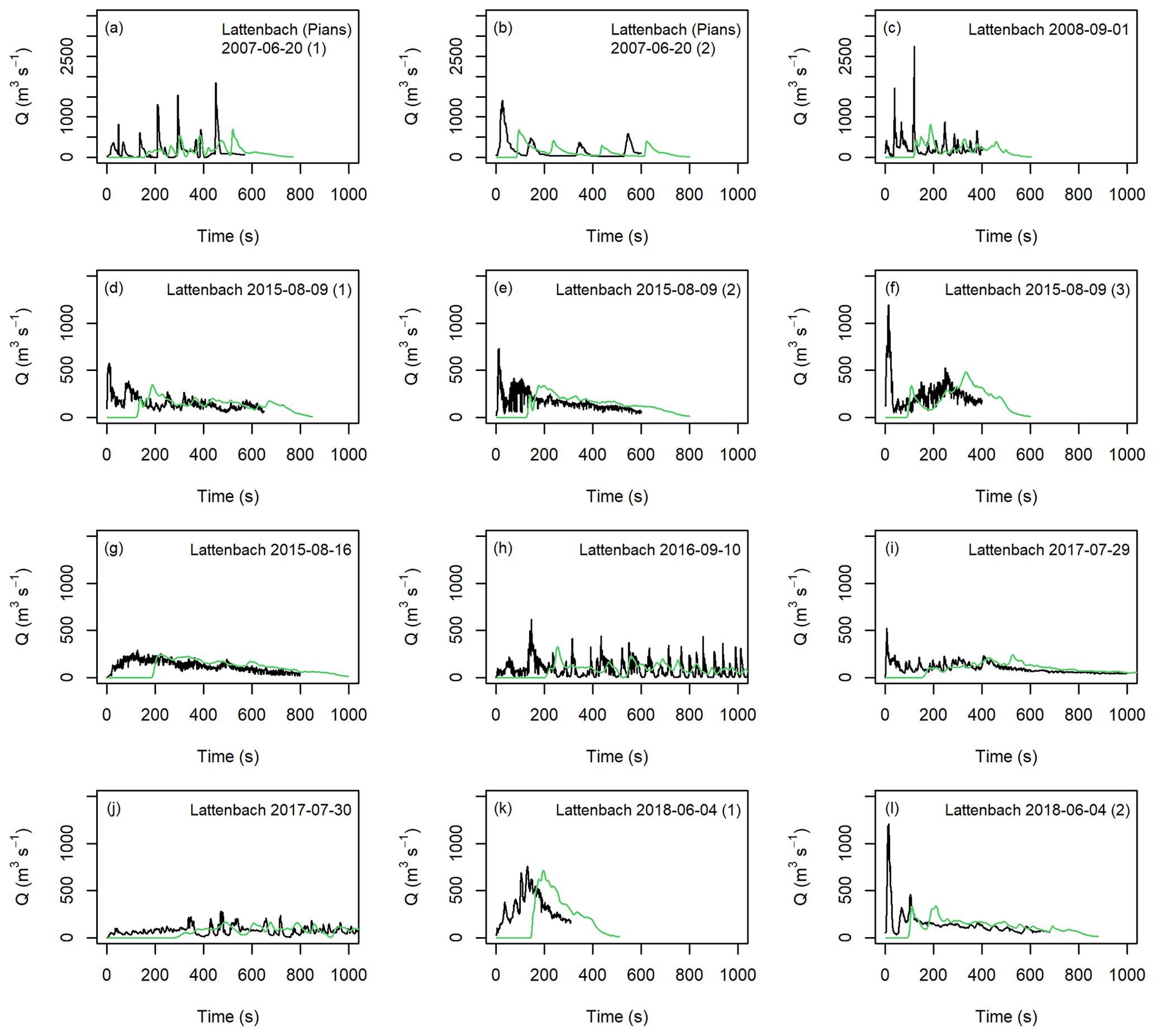
Figure 8Comparison of input hydrographs (black lines) from the Lattenbach site and extracted hydrographs at x=1000 m in the numerical experiment (green lines). Note the different y-axis range for panels (d) through (l) compared to panels (a) through (c).
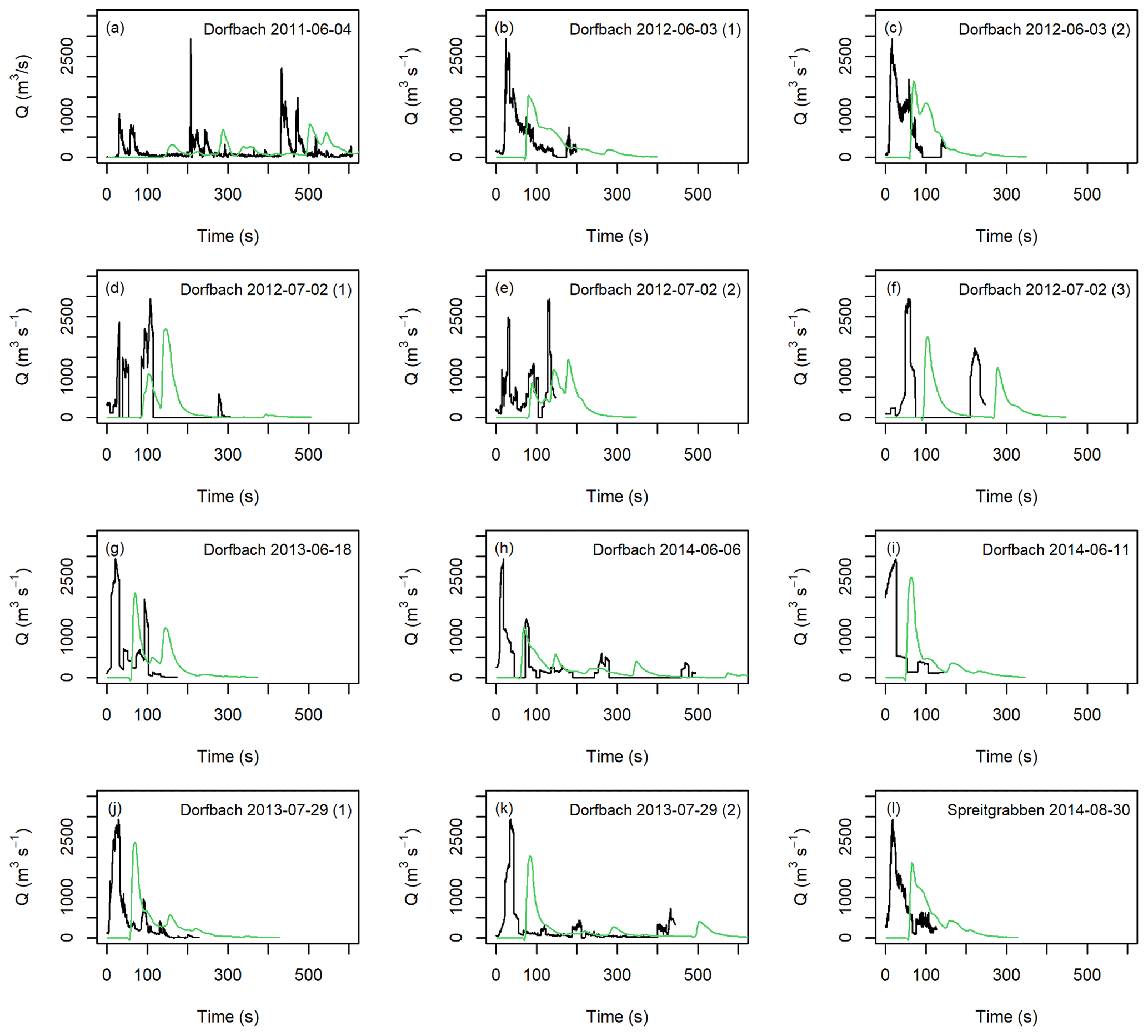
Figure 9Comparison of input hydrographs (black lines) from the Dorfbach and Spreitgraben sites and extracted hydrographs at x=1000 m in the numerical experiment (green lines).
Flow intensity indicators (depth, velocity, and IDF) were sensitive to the inflow conditions at four locations along the channel (Fig. 10). The sensitivity and variability in the maximum flow depth and IDF decreased with increasing distance down the channel. We attribute this to the material decelerating on the lower channel, implying the maximum depths are related to the final thickness of material. Since IDF is calculated with the square of velocity, as the velocities decreased, the variability in IDF related to variability in velocity also decreased. The cases with higher Qp and lower inflow duration tended to have greater maximum depth, velocity, and IDF; however, both relationships have significant scatter, as shown in the Appendix (Figs. A6 and A7).
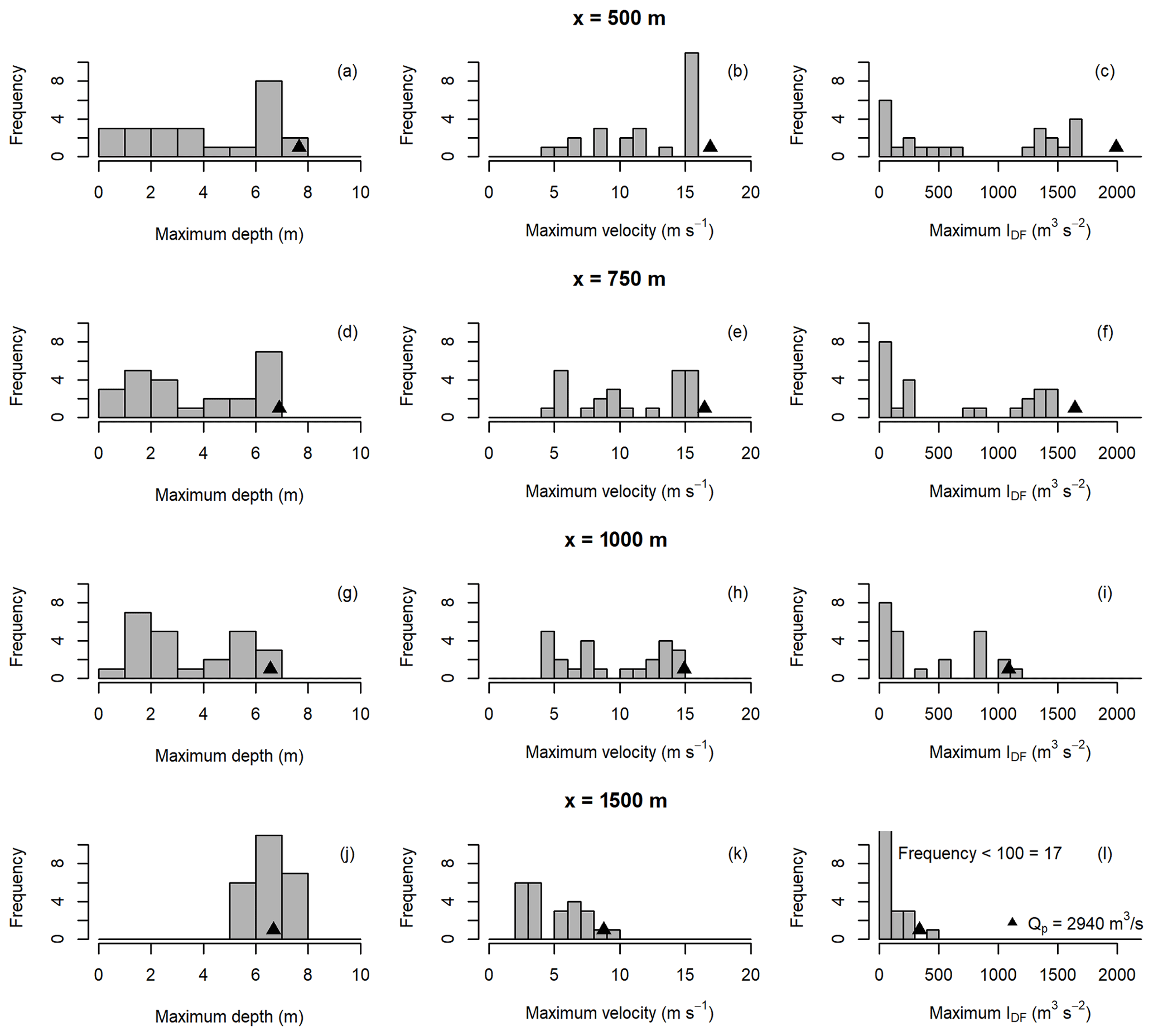
Figure 10Comparison of modelled flow intensity indicators using consistent Voellmy parameters (f=0.2, ξ=200 m s−2). Histogram bars indicate the distributions for the 24 real hydrographs modelled, all scaled to a volume of V=100 000 m3 and peak discharge of Qp≤2940 m3 s−1. The single triangle points represent the results from the triangular hydrograph input.
In the previous section we detailed how variations in flow resistance and inflow conditions affected debris-flow depth and velocity using an idealized synthetic topography. In this section, we apply the scaled, real hydrograph inputs to the much more complex topography of two natural debris-flow sites in southwestern British Columbia, Canada.
5.1 Currie D
There are four debris-flow fans on the north slope of Mount Currie, referred to as Currie A through D. The site is located approximately 4 km southeast of Pemberton, BC, Canada. The simulations shown here are for the eastern-most fan, Currie D, which has a watershed area of 1.7 km2 and extensive talus slopes composed of granitic rocks in the source area. A debris flow occurred on Currie D sometime between 3 and 12 July 2019, with a deposit volume of 100 000 m3 ± 5000 m3 (Zubrycky et al., 2021a). Zubrycky et al. (2021a) calculated the volume using lidar change detection with pre-event topography from 2017 and post-event topography collected in October 2019 utilizing a UAV-lidar system. Deposit mapping and UAV-lidar data for this event are available online (Zubrycky et al., 2021b). One velocity estimate from a superelevation calculation, two estimates of maximum flow depth, and two estimates of final deposit depth are from a field survey of the site in October 2019 (Fig. 11).
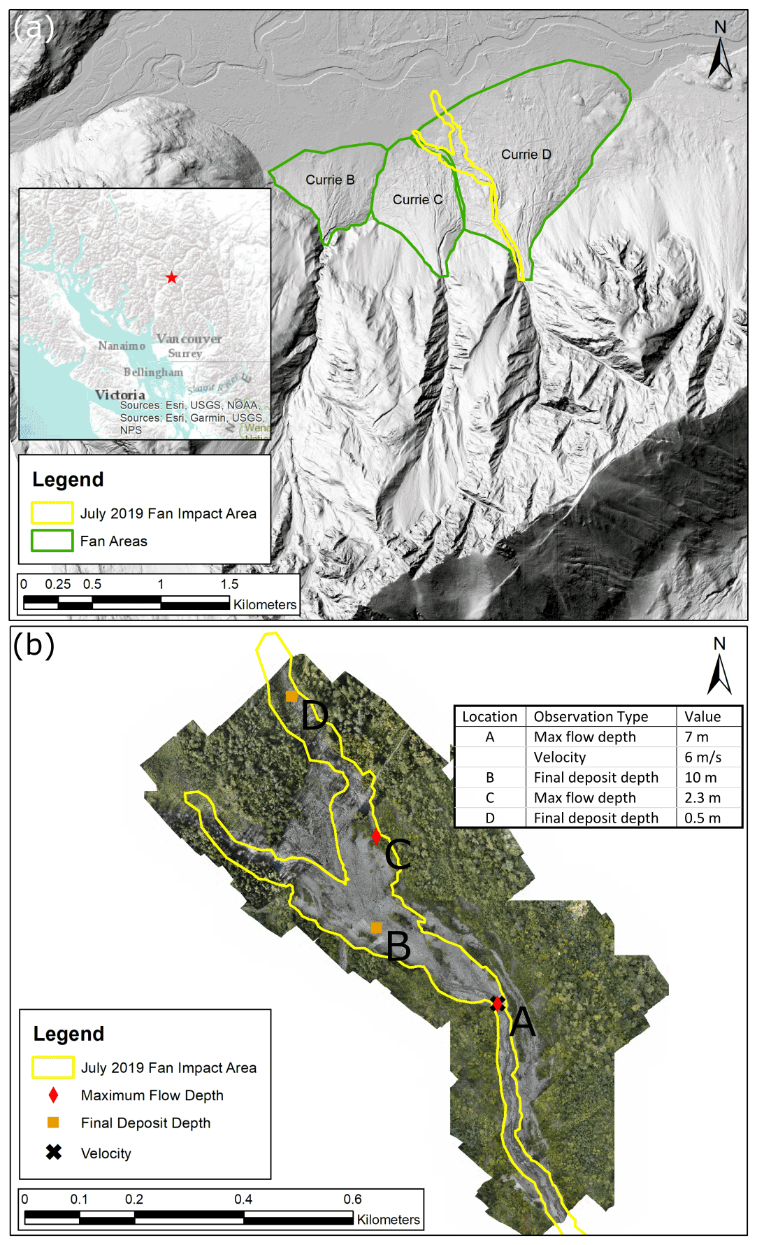
Figure 11Currie D 2019 impacts. Hillshade derived from pre-event (2017) lidar data provided by the Squamish-Lillooet Regional District (a) and post-event orthophoto obtained from the 2019 UAV survey (b).
The inflow location was set near the fan apex, where local channel slope was 44 % (24∘). We used a friction parameter of f=0.13 based on a preliminary calibration, without variable-inflow conditions, to approximately match the event runout and three values of the ξ parameter. By varying the hydrograph inputs and Voellmy parameters, we observed variability in the simulated flow depths, deposit depths, and velocities at the points of the field observations (Fig. 12). The results for the area impacted are aggregated in the impact proportion plots in Fig. 12a–c. The proportion of cases impacting an area is represented as filled contours, with a value of 1 indicating all 24 simulations impacted that grid cell and a value of 0 indicating no impacts in any simulation. In the impact proportion plots, the area along the main channel was consistent between all input hydrographs and flow-resistance parameters; however, the three flow-resistance cases presented show slightly different avulsion patterns. The simulation results at the observation points (consistent with the field observations shown in Fig. 11) are shown in Fig. 12d–o.
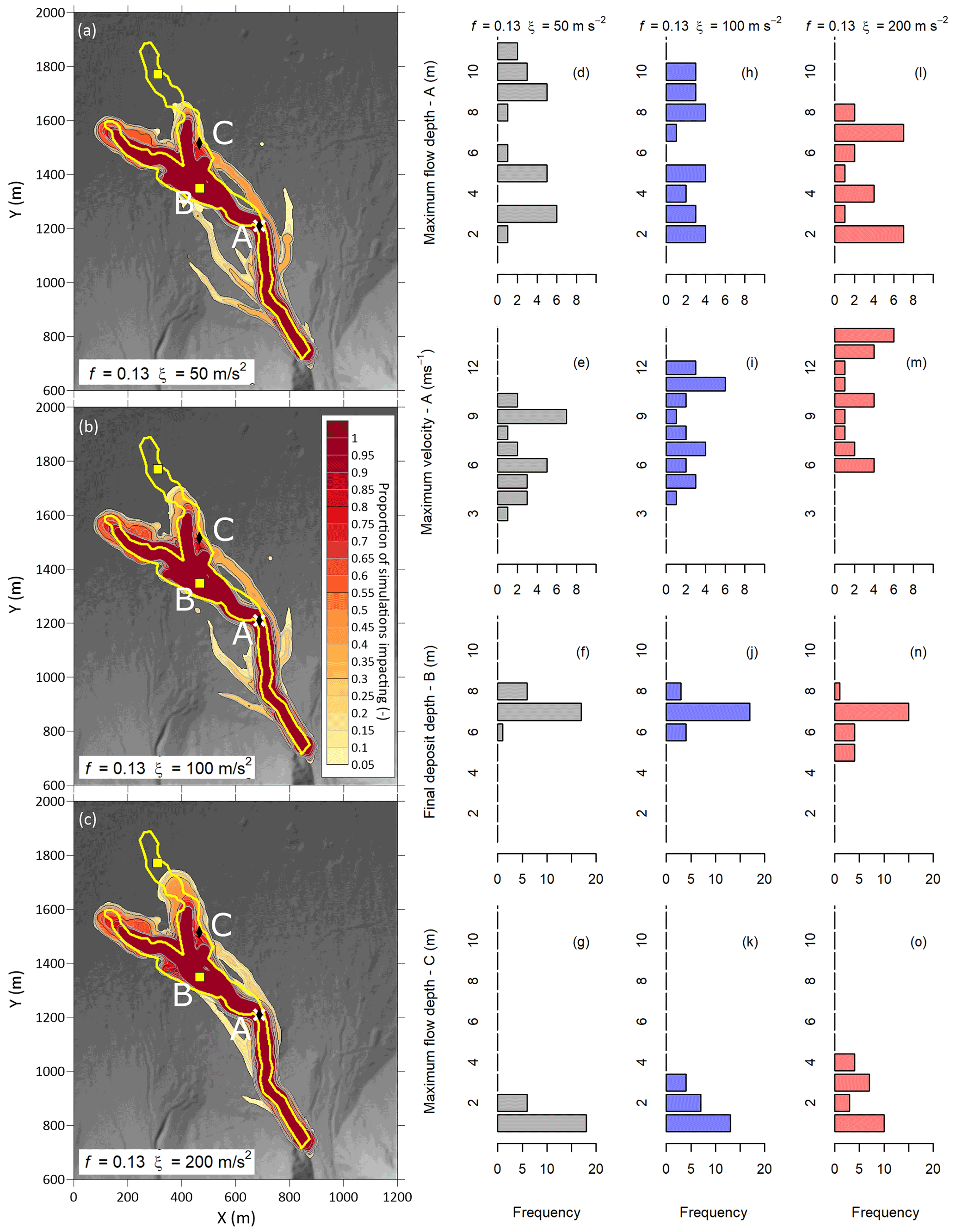
Figure 12Variability in impact (a–c) and intensity (d–o) using 24 real hydrographs and three sets of Voellmy parameters. Topographic data derived from pre-event (2017) lidar data provided by the Squamish-Lillooet Regional District. The yellow outline on the impact proportion plots (a–c) indicates the observed impact area from the actual event.
Our results show some sensitivity to the velocity-dependent resistance, ξ; however, the results are generally much more sensitive to the variability in the inflow conditions, particularly higher in the channel. As with the results for the numerical flume, the variability decreases downslope as the material slows and deposits. Numerical results for each observation are provided in the Appendix, separated by input hydrograph (Tables A2 through A4). Similar to the results for the numerical flume, the highest depths and velocities tend to correspond to the largest peak discharges; however, there is significant scatter in that relationship.
5.2 Neff Creek
Neff Creek is located approximately 25 km northeast of Pemberton, BC, Canada. A large debris flow occurred on the Neff Creek fan on 20 September 2015, with an estimated deposit volume of 220 000 m3 ± 30 000 m3 (Zubrycky et al., 2021a). The debris flow was triggered during a large-storm event following a dry summer (Lau, 2017). The event was characterized by significant erosion on the fan, with an estimated 40 % of the event volume entrained from the upper and medial portion of the fan and erosion depths of up to 14 m (Lau, 2017). The watershed area is 3.3 km2, and the source material is composed of sedimentary rocks.
Maximum flow depths and deposit depths on the lower fan were based on field estimates and change detection analysis for a portion of the fan (pre-event data from 2011 and post-event data from 2015) to check the deposit estimates. The impact area was mapped using satellite imagery (Fig. 13) and a field survey and is available online (Zubrycky et al., 2021b). Field observations of overlapping deposit lobes suggested that some material deposited during the event led to multiple avulsions and widening of the deposits. For the simulations, we selected the inflow location on the mid-fan, approximately where the event changed from being primarily erosional to primarily depositional, to avoid the added complexity of considering entrainment within the simulation. The local channel slope at the inflow location was 29 % (16∘).
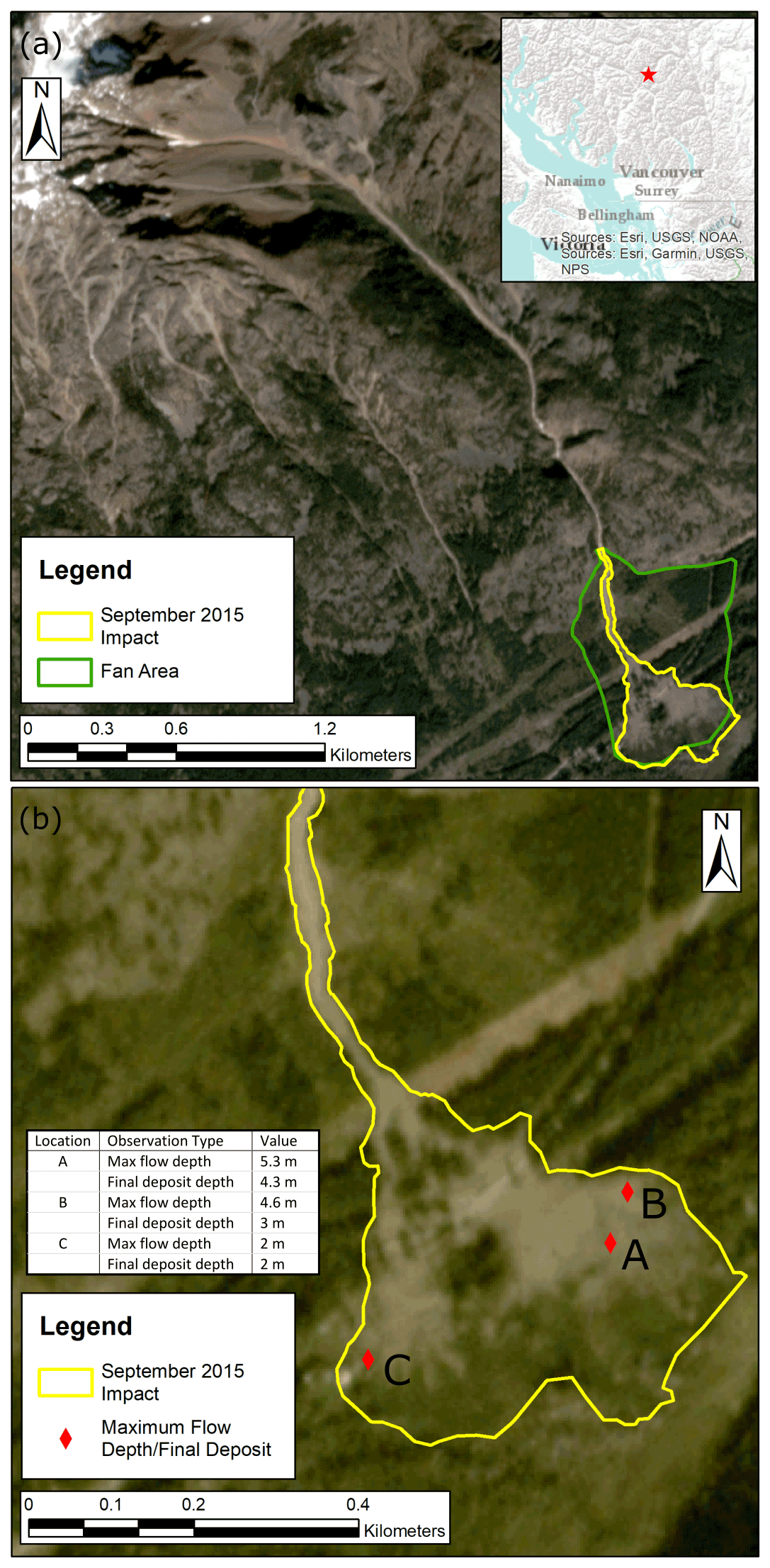
Figure 13Neff Creek 2015 impacts. Background imagery from Planet Inc. (2021).
In this study, we initially ran a set of simulations using Voellmy parameters f=0.10 and ξ=365 m s−2, calibrated assuming a single surge condition by Zubrycky et al. (2019), with 24 input hydrographs scaled with a c value of 0.2. We refer to these simulations as the variable-inflow case (Case 1). We then completed 10 iterations using the Monte Carlo sampling and deposition between runs outlined in Sect. 2.4 for the deposition-during-flow simulations (Case 2). Finally, we considered deposition with two materials (Case 3). For this case, we followed the same procedure as the deposition-during-flow case to modify the topography between flow stages but randomly assigned f=0.18 and ξ=365 m s−2 to 25 % of the particles to simulate the effect of heterogeneous flow resistance within an event. The results of these analyses are presented in Fig. 14.
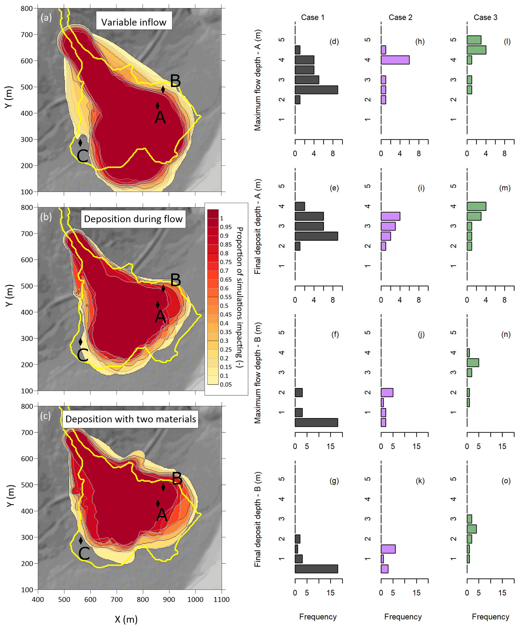
Figure 14Variability in impact (a–c) and intensity (d–o) for the different Neff Creek simulations. The yellow outline on the impact proportion plots (a–c) indicates the observed impact area from the actual event. Topographic data derived from pre-event lidar data provided by BC Hydro. Results at Point C are not shown because the simulated maximum flow and final deposit depths were less than 0.5 m for all simulations.
Case 1 systematically underpredicts lateral runout extents, as well as flow and deposit thickness, at the field observation locations (Fig. 14). Cases considering deposition during an event resulted in greater lateral spreading, shorter runout distances, and thicker flow depths and deposits at the observation points, all of which are more consistent with the field observations than the single-hydrograph-input cases. The deposition cases have fewer runs than the variable-inflow case, but each run for the topography modification cases consisted of four randomly sampled hydrographs and stage volumes. This variation within each simulation could contribute to the increased variability at the observation points, despite having fewer runs total.
Most numerical modelling studies of debris flows focus on model definition, material, or flow-resistance properties. At the same time, studies from instrumented debris-flow catchments have demonstrated the large variability in discharge that occurs in natural debris flows. In this study, we incorporated the natural variability in debris-flow discharge as an input for an equivalent-fluid numerical runout model. In doing so, we provide a first step towards understanding the interactions between inflow hydrographs, topography, and flow resistance within a single-phase, equivalent-fluid model.
This study utilized a SPH framework for the numerical modelling. Some of the development, such as the method for discretizing the inflow hydrograph into particles, is specific to a SPH model. However, many of the interactions between inflow and the downstream dynamics are expected to be applicable to other equivalent-fluid models. Future research using real hydrograph inputs with other single-phase numerical models, as well as with multi-phase numerical models that allow for hydrograph inputs, could provide insight into how sensitive these behaviours are to varying inflow (similar to comparisons done at the JTC1 Workshop; Pastor et al., 2018).
6.1 Topography and flow-resistance effects
Our modelling results highlight the topographical and flow-resistance sensitivities of peak discharge estimates. We evaluated the interplay between Voellmy parameters and channel slope in a controlled manner using the numerical flume model topography. Figures 5 and 6 illustrate that the peak discharge is insensitive to the Coulomb friction parameter (f) at values lower than the channel slope but that peak discharge rapidly decreases as the channel slope becomes equal to or greater than the f value. This is an intuitive result as the best-fit f value in a Voellmy model can generally be estimated by the local slope where material deposition begins. The results also show that peak discharge increases as the velocity-dependent resistance parameter (ξ) increases, and the sensitivity to ξ increases with increasing peak discharge, all other factors equal. The positive correlation with peak discharge is expected as ξ generally controls the flow velocity, with higher ξvalues generating higher velocities.
The simulated peak discharges tend to decrease as the channel slope decreases (Figs. 5 and 6). The implication of this finding is that, when defining inflow conditions to calibrate the model to an observed debris-flow event where there is a downstream peak discharge estimate, the inflow peak discharge will have to be either equal to or greater than the downstream estimate if a single flow resistance is used. If the channel slope is steeper than the f value along the channel leading to the point where a discharge estimate is obtained, the downstream estimate peak discharge could be directly used as the inflow peak discharge upstream. However, if the local channel slope is near to or lower than the f value, the hydrograph will attenuate, and a higher inflow peak discharge will be necessary to match the downstream discharge observation. The exact value of the f parameter where significant attenuation will occur also depends on the ξ value used, with lower values of ξ leading to higher attenuation in the hydrograph. For example, the modelled peak discharge is approximately equal to the inflow peak discharge for all cases shown in Fig. 5a and b where the local channel slope is greater than the f value. Further in the simulation, the peak discharge attenuates significantly where the local channel slope is less than the f value (Fig. 5e) relative to the inflow hydrograph and the case where the local channel slope is still greater than the f value (Fig. 5d). Taken together, this suggests that, when calibrating a numerical runout model to a peak discharge estimate or using a design peak discharge estimate for forward analysis, the topography between the inflow location and the location of interest has an effect on the simulation. Furthermore, the effects of the flow-resistance parameters and the topography are interconnected.
6.2 Effects of variable inflows
We selected 24 inflow hydrographs from discharge-versus-time records for 21 debris flows observed in 3 natural channels. The observed discharge over time for each of these events arose from a unique combination of watershed conditions, triggering conditions, channel geometry, and measuring locations. Watershed characteristics and channel geometries are more or less constant for the records of multiple events from the Lattenbach site, and the same applies to the Dorfbach site. However, even with these two factors controlled, there was significant variability within the measured hydrographs at these sites (Table 1), which highlights the challenge of attempting to estimate a realistic inflow hydrograph for a runout analysis. The approach taken in this study is to use these real-event records as an indication of the potential variability in the inflow conditions that could occur while recognizing that they will not be exact analogs for events in other locations. Field monitoring of debris-flow discharge is becoming more common (Hürlimann et al., 2019), and collecting more of these data at more locations could provide valuable information for future modelling, allowing for a more refined selection of input hydrographs based on site-specific information.
We demonstrated the effect of changing inflow conditions based on the 24 inflow hydrographs by running each hydrograph through the idealized model geometry and extracting flow intensity metrics, consistent with those commonly used in hazard assessment or mitigation structure design. Flow depths, velocities, and impact intensities (as defined by Jakob et al., 2012) varied significantly (Fig. 10), and variability decreased as distance from the input location increased. The disaggregated results provided in the Appendix (Figs. A6 and A7) show that simulations with higher Qp and lower inflow duration tend to have higher impact intensities; however, there is significant scatter, suggesting that the variability is affected by other characteristics of the inflow hydrograph. When compared to the results using a simple, triangular hydrograph input, the maximum simulated flow depth, velocity, or intensity index for any case generally corresponded to the triangular hydrograph with a peak discharge set at the maximum allowable for the real hydrographs. This suggests that, when modelling flow intensities in channelized conditions, a triangular input hydrograph provides an adequate estimate of maximum intensity.
6.3 Case histories
We examined two case histories, Mount Currie D from 2019 and Neff Creek from 2015, both in southwestern BC, Canada, using variable inflows based on the real hydrographs described in this study. The objective of the modelling was not to find the specific hydrograph input that resulted in the best match to the observed deposits but rather to examine the variability in impacts arising from the natural variability in discharge from the inflow hydrographs. The simulated flow intensities showed considerable variation, even with consistent Voellmy parameters (right panels in Figs. 12 and 14); however, the variation decreased towards the distal end of the deposit, which is consistent with the results from the idealized topography (Fig. 10).
The impact proportion plots for Currie D (left panel in Fig. 12) show distinct patterns of avulsions for the simulations with different ξ values. We attribute this behaviour to the channel being overwhelmed in the cases with lower ξ, which are slower, versus material leaving the channel after superelevating around bends with higher ξ. Along with the difference in avulsion locations, there were fewer avulsions with higher ξ. The simulations of the Neff Creek event showed the limitations of the variable-inflow conditions, with a consistent underprediction of the lateral extents and overprediction of the runout length of the event (Fig. 14), consistent with the single-surge results presented by Zubrycky et al. (2019). To overcome this limitation, we modelled a multiple-phase event, where the previous phases would modify the topography. This approach is reasonable as the observations from the real debris flows summarized in Table 1 indicate several instances of multiple debris flows within 1 d, modifying the topography for subsequent surges. We achieved a better match to the observed event by modelling the topographic modification. There are practical challenges to applying this topography modification method to a forward analysis as the number of phases where deposition will occur must be selected, increasing the number of model runs and model complexity. In the examples shown, considering 10 runs with random combinations of volume and inflow conditions resulted in a reasonable trade-off between capturing variability and runtime (the runtime for 10 runs with 4 phases each was approximately 32 h).
With the idealized topography, we found that a higher-resistance flow front amplified the peak discharge (Fig. 7). This approach demonstrates the idea of a coarse flow front leading to surging behaviour. The effect of mixing particles within a flow was also tested in the Neff Creek case study. Adding in a higher-resistance material with the f value approximately equal to the channel slope upslope of the roadway resulted in greater variation in deposit area and depths and enhanced the runout distance relative to the variable-inflow-with-deposition case. This increase in mobility is somewhat counter-intuitive, with 25 % of the particles having a higher frictional resistance. This result may be related to the higher-resistance particles maintaining higher flow depths, resulting in larger driving stresses within the flow. Future research could be conducted to examine how multiple flow-resistance particles mixed within a simulation can be used to represent flow behaviours more realistically.
6.4 Selection of inflow conditions and peak discharge
We examined the sensitivity of the model results to assumptions regarding the location and velocity of the material entering the model. We found that there may be some numerical instability related to the smoothing length calculation early in the model, when only a small fraction of the particles have entered the model domain, or from initial accelerations or decelerations of the particles as they enter the model. We recommend placing the inflow location far enough upstream of any observations of interest to allow the simulated flow to “spin up”. We found that a distance of approximately 250 m upslope of the areas of interest had stable model results with little sensitivity to inflow location (e.g., Figs. A3 and A4); however, this is likely not a fixed value and will depend on the topography and flow characteristics in a given case.
We implemented a scaling method that used the shape of the observed hydrographs but allowed for a user-defined volume and peak allowable discharge. The empirical relationship to estimate peak allowable discharge (Eq. 5) is commonly used, and there is existing guidance for selecting the c parameter based on the debris-flow source material (Rickenmann, 1999; Ikeda et al., 2019). The data used to fit the regression between event volume and peak discharge are very scattered, and a wide range of c values fit a region of those data (Rickenmann, 1999; Ikeda et al., 2019), which limits the confidence in any specific peak discharge estimate. Despite this limitation, we used Eq. (5) because it provides a simple method to define an allowable peak discharge for the scaled hydrographs.
6.5 Limitations
There are sources of uncertainty and simplifications relating to the modelling approach and field observations that should be considered when interpreting the results presented here. The single-phase, equivalent-fluid model used in this study considers the heterogeneous debris flow to be a fluid governed by simple flow-resistance models. Other models that consider solid and fluid motion independently still do not consider all the materials present in a flow, such as large woody debris or individual large boulders that can have an important influence on flows, for example, by creating channel blockages.
We applied hydrographs from specific locations to sites in different hydroclimatic and geomorphic settings. There is uncertainty associated with the field measurements, and the level of uncertainty is different for each field measurement. For example, the estimates of maximum flow depths are dependent on the observation of mud lines above the final deposit and the depth of the final deposit. The uncertainty in the final deposit depth is dependent on the quality of pre- and post-event topography data. Due to the complexity of variability in the natural systems leading to debris-flow events, our approach provides a practical way to explore the potential variability in debris-flow outcomes. When applying this approach to forward analysis, the significant uncertainty in the volume and mobility of future events must be recognized as these factors can vary widely, even at a single channel.
A further limitation of this work is that entrainment is not considered. Entrainment not only affects the volume of an event but also influences the dynamics through momentum transfer between the erodible bed and the flowing material as well as modification of effective basal resistance (Iverson and Ouyang, 2015). Future work could consider how entrainment interacts with these processes. Similar to the Monte-Carlo-type random sampling employed for the deposition within event cases for Neff Creek, a similar approach could be taken to also consider different entrainment rates. While this approach is computationally intensive, computational techniques such as GPU processing could significantly reduce runtimes and make large Monte Carlo simulations feasible for geohazard practitioners.
We have demonstrated how variable-inflow conditions, based on real observations of debris-flow events, can result in variability in numerical runout model results. We developed a modified version of the Dan3D runout model that allows for a hydrograph input. We tested the interactions between topography, Voellmy parameters, and inflow conditions for an idealized model topography. This approach demonstrated the combinations of inflow conditions and flow-resistance parameters that can lead to relatively steady flow, peak discharge attenuation, or peak discharge amplification. Using an idealized model topography, we showed that scaled, real hydrograph inflows with constant Voellmy parameters resulted in significant variation in the simulated flow depths, velocities, and impact intensities. These variations were greatest in the steeper sections of the topography and decreased on the shallower, distal runout portion of the simulations. A triangular input hydrograph provided an adequate estimate of maximum intensity for the channelized conditions. We found similar results using the real hydrograph inflows when applied to real topography for two case histories from southwestern BC. In the case of Mount Currie D, the variation in simulated flow depths and velocities was greater because of the variable inflows as compared to varying Voellmy parameters. For the simulation of Neff Creek, the results matched the observed event behaviour more closely when variable inflow was coupled with deposition between event phases. These results demonstrate how considering variation in inflow conditions can lead to reasonable estimates of the potential variation in event impacts. Our work shows the utility of considering inflow conditions, with many opportunities for future work to advance the application of these ideas in practical predictive modelling by geohazard practitioners.
An input file with the input time, position, volume, velocity, and material code for each of the 4000 particles is generated. The general process for defining the model inputs is shown in Fig. A1 for a triangular hydrograph with V=10 000 m3 and Qp=500 m3 s−1, tp=8 s, and tin=40 s.
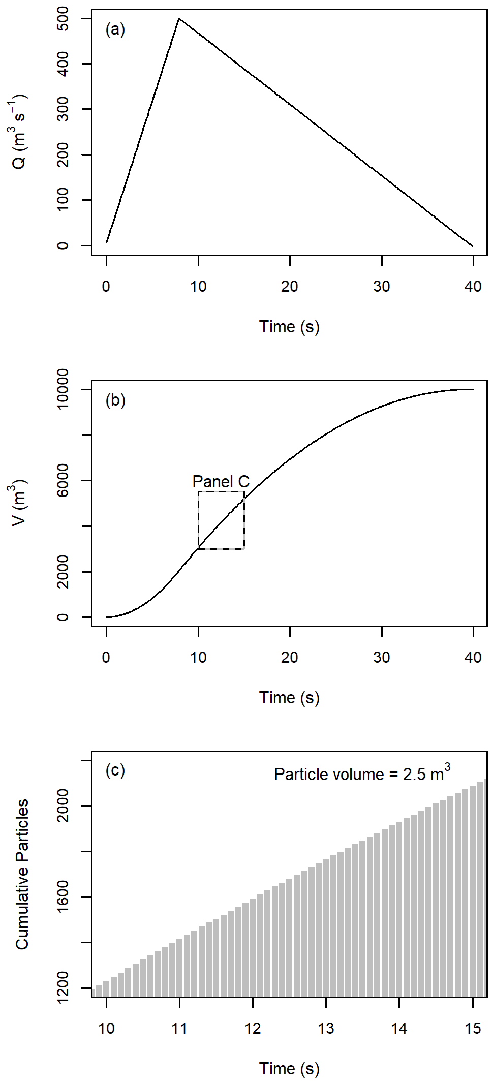
Figure A1(a) Input hydrograph, (b) cumulative volume in the model versus time, and (c) discretization of the cumulative volume into simulation particles for the portion of the time series indicated in (b).
.
The effect of smoothing the raw hydrograph results is shown in Fig. A2. The shape and peak discharge of the results are preserved, but small oscillations in the discharge time series are removed.
The sensitivity of the calculated peak discharge at x=1000 m to the inflow location is shown in Fig. A3. For ease of visualization, only the minimum and maximum values of the velocity-dependent resistance parameter tested are shown (25 and 500 m s−2, respectively) as all other values will plot between the ones shown. The calculated peak discharge has a low sensitivity to the inflow location as the calculated peak discharges are all similar when the same Voellmy parameters are used.
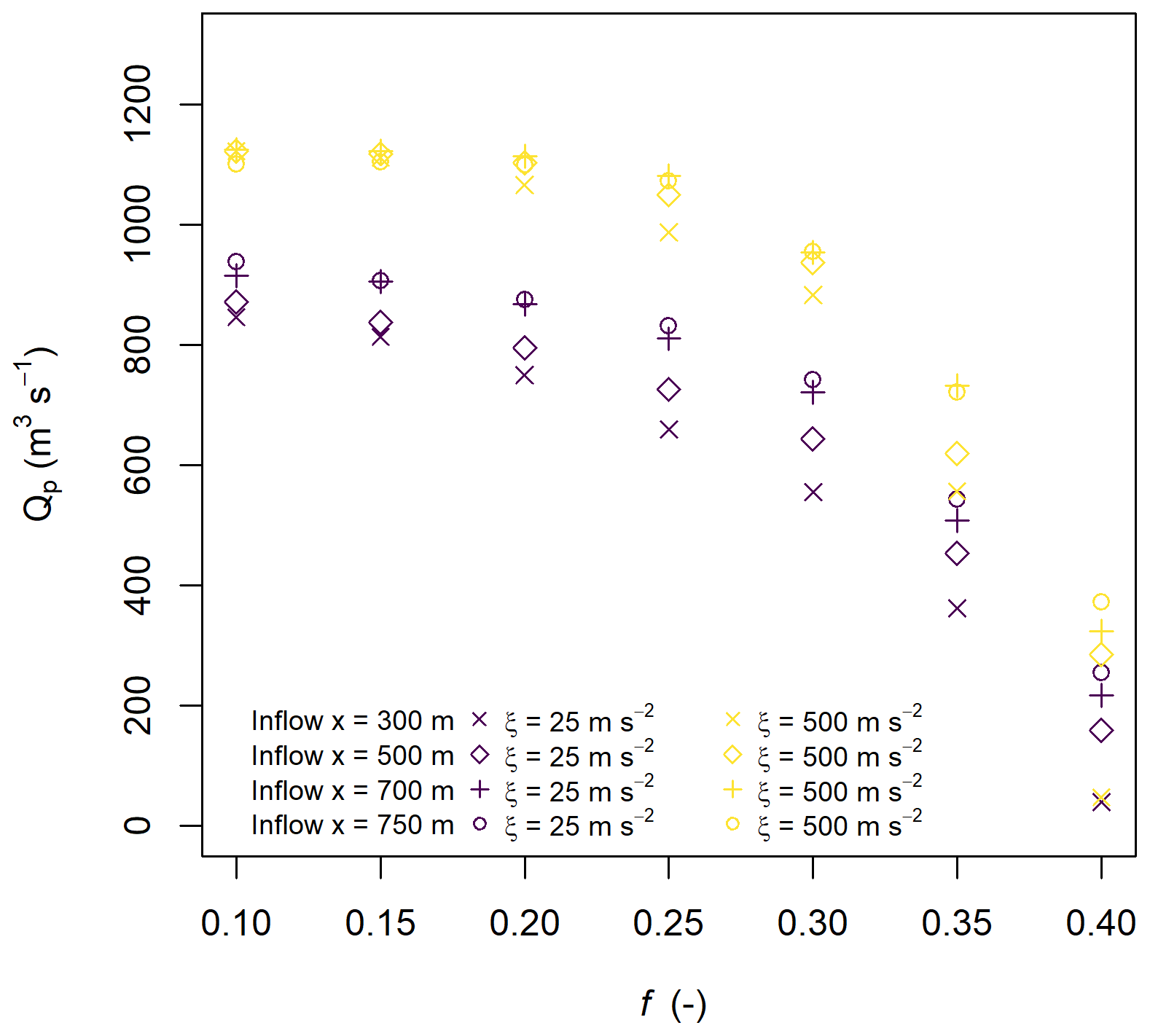
Figure A3Sensitivity analysis for peak discharge at x=1000 m for different inflow locations.
The sensitivity of the calculated peak discharge to the initial velocity was tested by comparing the results of simulations using Eq. (6), to define the initial velocity, to results of simulations using all particles with a constant velocity of either 5, 10, or 15 m s−1. All simulations were run with Voellmy parameters f=0.2 and ξ=200 m s−2, as shown in Fig. A4. There is a negligible difference between the simulations shown, indicating that the choice of initial velocity has little impact on the simulations.
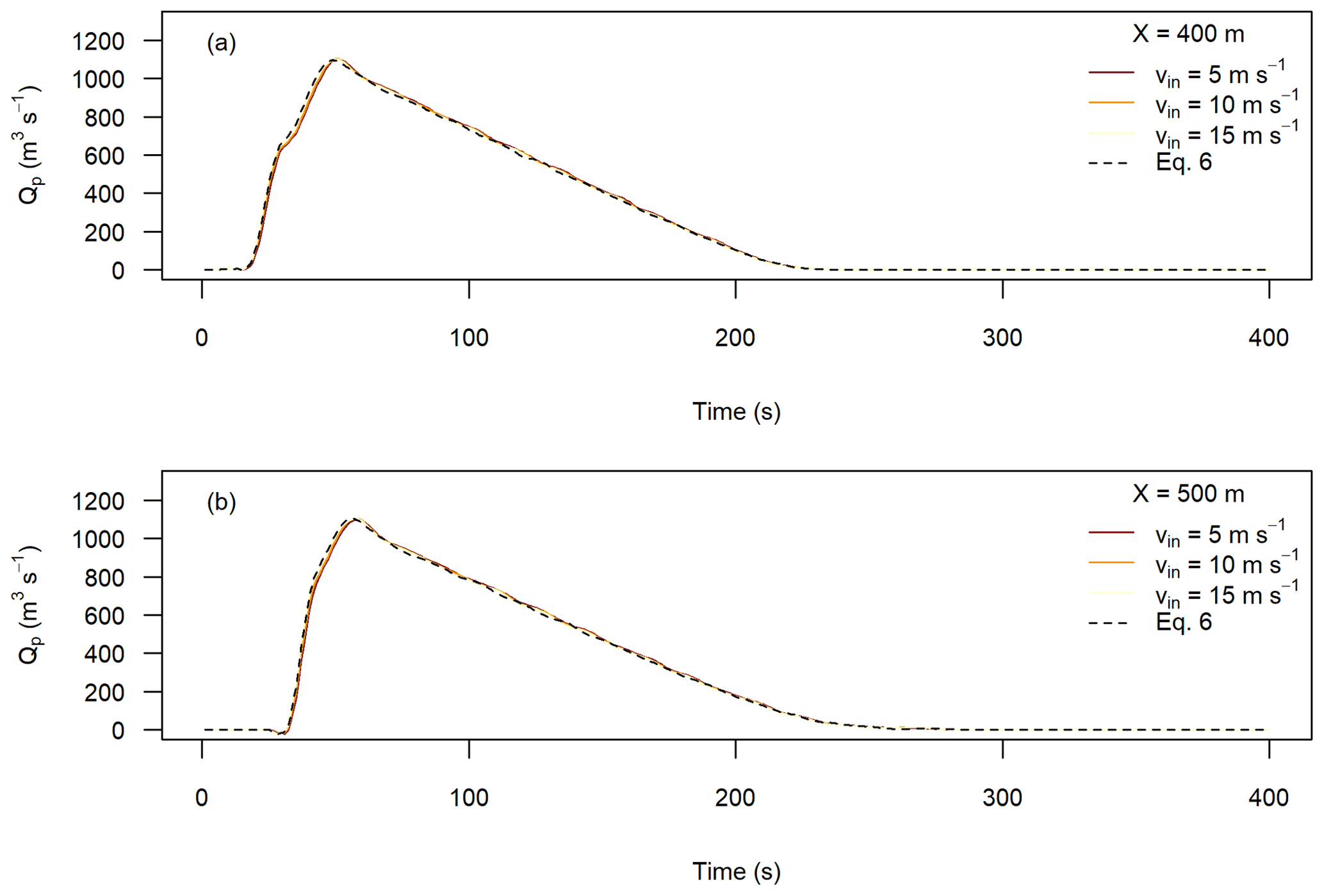
Figure A4Sensitivity to initial velocity using the numerical flume with particles added at x=300 m.
The results for the flow depth, velocity, and IDF from the simulation of the scaled, real hydrographs in the numerical flume were plotted against the input peak discharge (Fig. A6). Similarly, the flow depth, velocity, and IDF were plotted against the total duration of the inflow hydrograph (Fig. A7). Hydrograph IDs are provided in Table A1. Greater input peak discharge and smaller inflow durations tend to result in greater flow depths, velocities, and IDF values; however, there is substantial scatter in all these relationships.
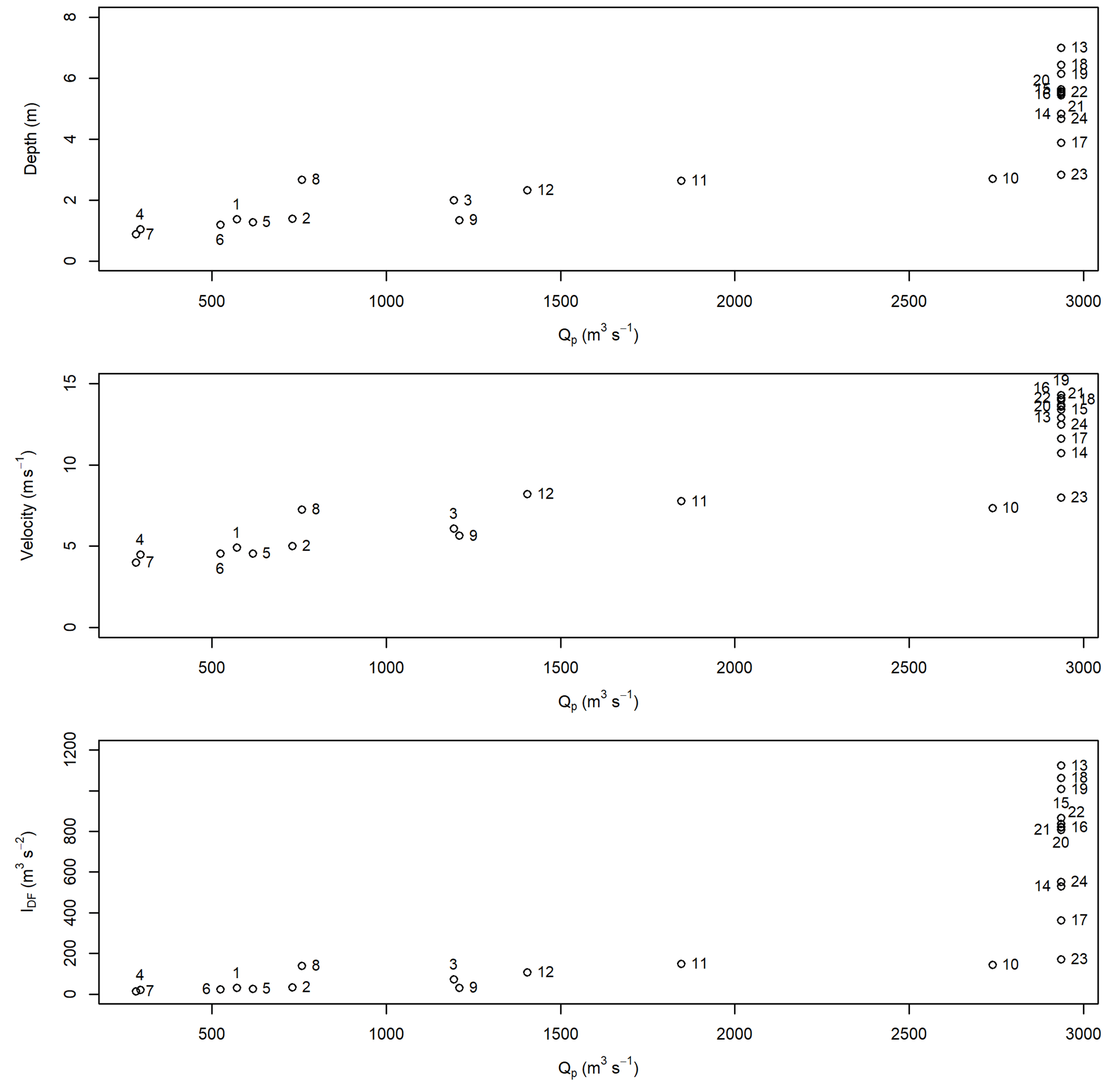
Figure A6Relationships between peak discharge and flow depth, velocity, and IDF for the numerical flume at x=1000 m. The numbers correspond to the hydrograph IDs summarized in Table A1.
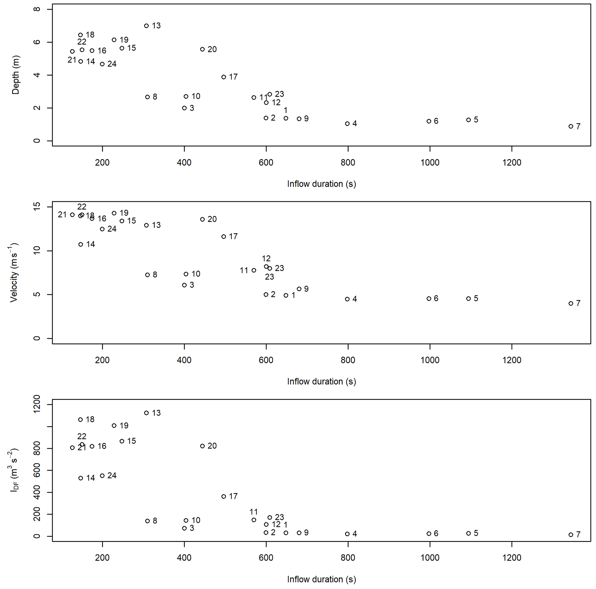
Figure A7Relationships between input hydrograph inflow duration and flow depth, velocity, and IDF for the numerical flume at x=1000 m. The numbers correspond to the hydrograph IDs summarized in Table A1.
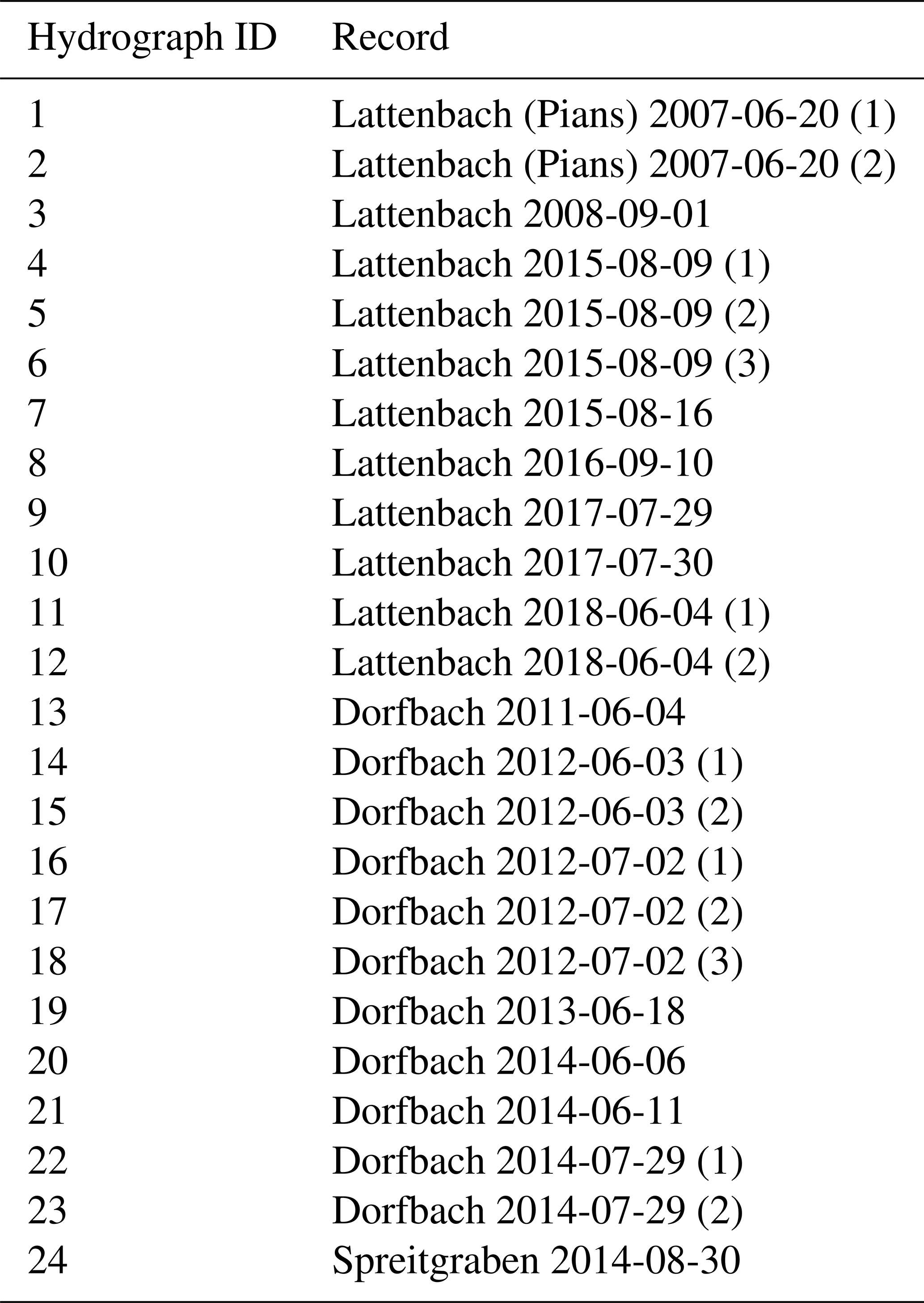
Table A2Summary of outputs for the Currie D simulations using f=0.13, ξ=50 m s−2.
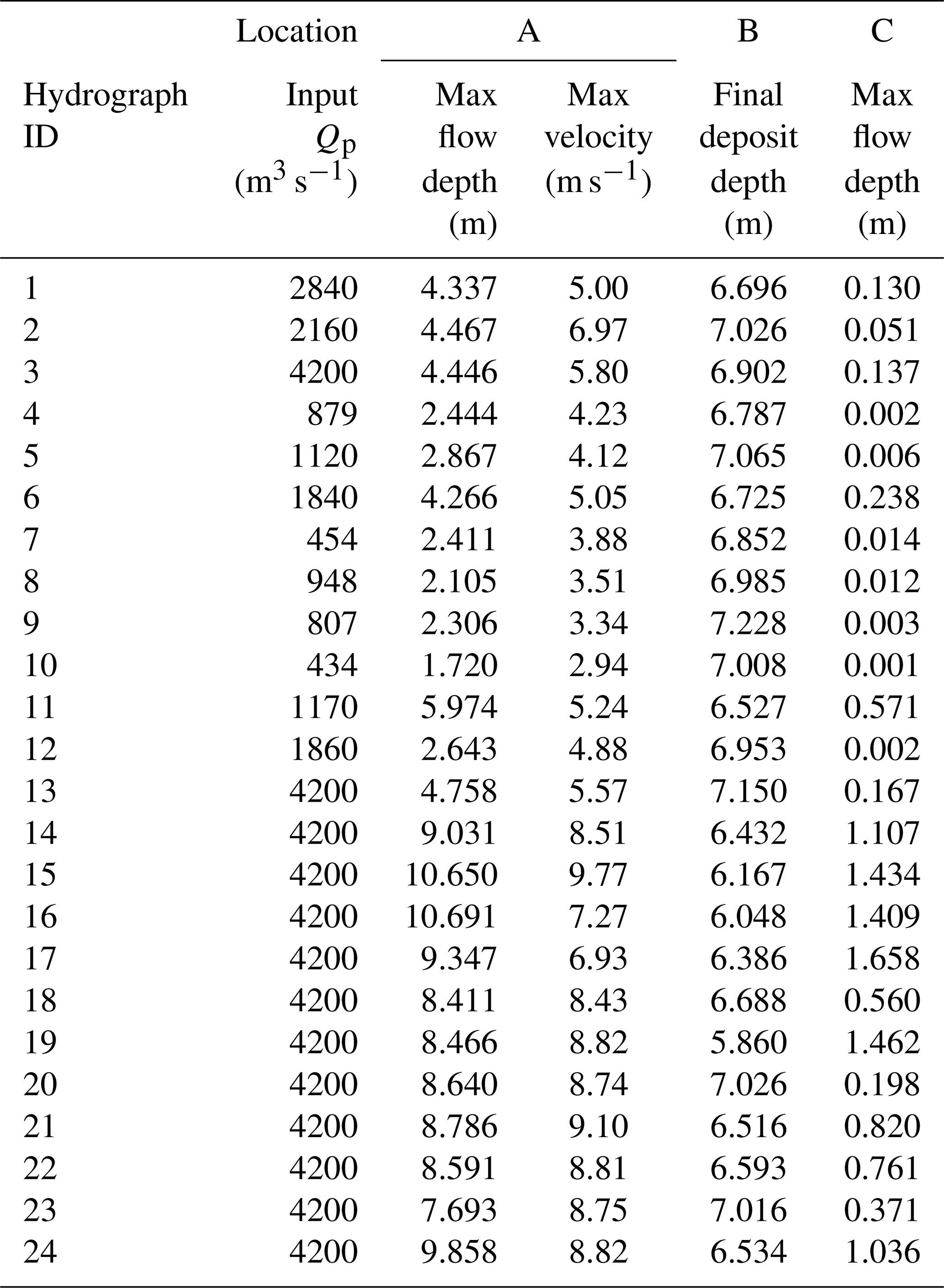
Table A3Summary of outputs for the Currie D simulations using f=0.13, ξ=100 m s−2.
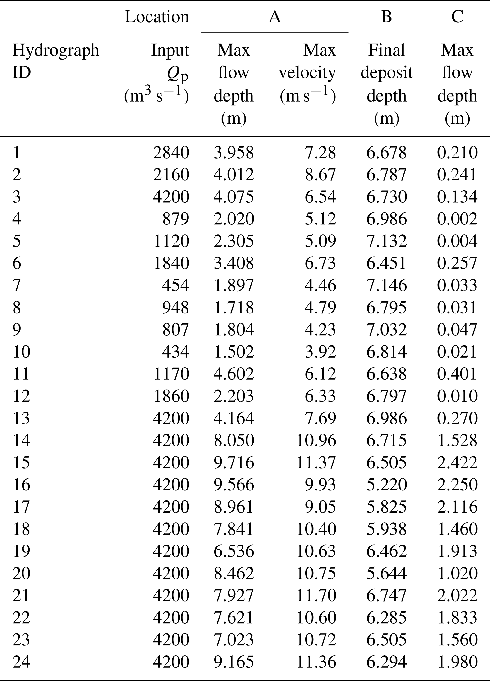
Table A4Summary of outputs for the Currie D simulations using f=0.13, ξ=200 m s−2.

Discharge-versus-time information for the real-event hydrographs in this study is available through the Pangaea repository: https://doi.org/10.1594/PANGAEA.943970 (Mitchell et al., 2022). A geodatabase of event mapping for the Mount Currie D and Neff Creek sites, as well as UAV-lidar data for Mount Currie D, is available through the Pangaea repository: https://doi.org/10.1594/PANGAEA.932864 (Zubrycky et al., 2021b).
AM contributed to conceptualization, BC field investigation, methodology, software development, analysis, and original draft preparation. SZ led the BC field investigation and contributed to review and editing of the manuscript. SM contributed to conceptualization, the BC field investigation, resources, and review and editing of the manuscript. JA provided support for software development and contributed to review and editing of the manuscript. MJ and CG curated data from the Swiss sites and reviewed and edited the manuscript. RK and JH curated data from the Austrian sites and reviewed and edited the manuscript. All authors participated in discussions on the study conceptualization and methodology.
The contact author has declared that neither they nor their co-authors have any competing interests.
Publisher's note: Copernicus Publications remains neutral with regard to jurisdictional claims in published maps and institutional affiliations.
We acknowledge the support of the Natural Sciences and Engineering Research Council of Canada (NSERC), funding reference number PGSD3–516701–2018, and the University of British Columbia, Four Year Fellowship no. 6456. This work has also benefited from conversations with Alex Strouth and Emily Mark of BGC Engineering on the subject of defining hydrograph inputs in practical situations. We would also like to thank Martin Mergili and Velio Coviello for their thoughtful and constructive reviews of this paper.
This research has been supported by the Natural Sciences and Engineering Research Council of Canada (grant no. PGSD3–516701–2018) and the University of British Columbia, Four Year Fellowship no. 6456.
This paper was edited by Daniele Giordan and reviewed by Velio Coviello and Martin Mergili.
Aaron, J., Stark, T. D., and Baghdady, A. K.: Closure to “Oso, Washington, Landslide of March 22, 2014: Dynamic Analysis” by Jordan Aaron, Oldrich Hungr, Timothy D. Stark, and Ahmed, K. Baghdady, J. Geotech. Geoenviron., 144, 07018023, https://doi.org/10.1061/(ASCE)GT.1943-5606.0001748, 2018.
Arai, M., Hübl, J., and Kaitna, R.: Occurrence conditions of roll waves for three grain-fluid models and comparison with results from experiments and field observations, Geophys. J. Int., 195, 1464–1480, https://doi.org/10.1093/gji/ggt352, 2013.
Bennett, G. L., Molnar, P. McArdell, B. W., and Burlando, P.: A probabilistic sediment cascade model of sediment transfer in the Illgraben, Water Resour. Res., 50, 1225–1244, https://doi.org/10.1002/2013WR013806, 2014.
Berti, M., Bernard, M., Gregoretti, C., and Simoni, A.: Physical interpretation of rainfall thresholds for runoff-generated debris flows, J. Geophys. Res.-Earth, 125, e2019JF005513, https://doi.org/10.1029/2019JF005513, 2020.
Bovis, M. J. and Jakob, M.: The role of debris supply conditions in predicting debris flow activity, Earth Surf. Proc. Land., 24, 1039–1054, https://doi.org/10.1002/(SICI)1096-9837(199910)24:11<1039::AID-ESP29>3.0.CO;2-U, 1999.
Chen, H. and Lee, C. F.: Numerical simulation of debris flows, Can. Geotech. J., 37, 146–160, 2000.
Chen, J.-C. and Chuang, M.-R.: Discharge of landslide-induced debris flows: case studies of Typhoon Morakot in southern Taiwan, Nat. Hazards Earth Syst. Sci., 14, 1719–1730, https://doi.org/10.5194/nhess-14-1719-2014, 2014.
Christen, M., Kowalski, J., and Bartelt, P.: RAMMS: Numerical simulation of dense snow avalanches in three-dimensional terrain, Cold Reg. Sci. Technol., 63, 1–14, https://doi.org/10.1016/j.coldregions.2010.09.006, 2010.
Coviello, V, Theule, J. I., Crema, S., Arattano, M., Comiti, F., Cavalli, M., Lucía, A., Macconi, P., and Marchi, L.: Combining instrumental monitoring and high-resolution topography for estimating sediment yield in a debris-flow catchment, Environ. Eng. Geosci., 27, 95–111, https://doi.org/10.2113/EEG-D-20-00025, 2021.
Dash, R. K., Kanungo, D. P., and Malet, J. P.: Runout modelling and hazard assessment of Tangni debris flow in Garhwal Himalayas, India, Environ. Earth Sci., 80, 338, https://doi.org/10.1007/s12665-021-09637-z, 2021.
Deubelbeiss, Y. and Graf, C.: Two different starting conditions in numerical debris-flow models – Case study at Dorfbach, Randa (Valais, Switzerland), in: Mattertal – ein Tal in Bewegung, Publikation zur Jahrestagung der Schweizerischen Geomorphologischen Gesellschaft, 29. Juni–1. Juli 2011, St. Niklaus, Eidg. Forschungsanstalt WSL, Birmensdorf, 125–138, https://www.dora.lib4ri.ch/wsl/islandora/object/wsl:11088 (last access: 27 April 2022), 2013.
Dowling, C. A. and Santi, P. M.: Debris flows and their toll on human life: a global analysis of debris-flow fatalities from 1950 to 2011, Nat. Hazards, 71, 203–227, https://doi.org/10.1007/s11069-013-0907-4, 2014.
Gregoretti, C., Degetto, M., and Boreggio, M.: GIS-based cell model for simulating debris flow runout on a fan, J. Hydrol., 534, 326–340, https://doi.org/10.1016/j.jhydrol.2015.12.054, 2016.
Hübl, J.: Ein einfaches Verfahren zur Bestimmung von Murgangabflüssen (A simple method to estimate debris-flow hydrographs), Wildbach- und Lawinenverbau, 188, 130–147, 2021.
Hübl, J. and Kaitna, R.: Monitoring debris-flow surges and triggering rainfall at the Lattenbach Creek, Austria, Environ. Eng. Geosci., 27, 1–8, https://doi.org/10.2113/EEG-D-20-00010, 2021.
Hungr, O.: Analysis of debris flow surges using the theory of uniformly progressive flow, Earth Surf. Proc. Land., 25, 483–495, https://doi.org/10.1002/(SICI)1096-9837(200005)25:5<483::AID-ESP76>3.3.CO;2-Q, 2000.
Hungr, O. and McDougall, S.: Two numerical models for landslide dynamic analysis, Comput. Geosci., 35, 978–992, https://doi.org/10.1016/j.cageo.2007.12.003, 2009.
Hungr, O., Leroueil, S., and Picarelli, L.: The Varnes classification of landslide types, an update, Landslides, 11, 167–194, https://doi.org/10.1007/s10346-013-0436-y, 2014.
Hürlimann, M., Coviello, V., Bel, C., Guo, X., Berti, M., Graf, C., Hübl, J., Miyata, S., Smith, J. B., and Yin, H.-S.: Debris-flow monitoring and warning: Review and examples, Earth-Sci. Rev., 199, 102981, https://doi.org/10.1016/j.earscirev.2019.102981, 2019.
Ikeda, A., Mizuyama, T., and Itoh, T.: Study of prediction methods of debris-flow peak discharge, in: 7th International Conference on Debris-Flow Hazards Mitigation, 10–13 June 2019, Golden, USA, 709–715, https://doi.org/10.25676/11124/173051, 2019.
Iverson, R. M.: The physics of debris flows, Rev. Geophys., 35, 245–296, https://doi.org/10.1029/97RG00426, 1997.
Iverson, R. M. and George, D. L.: A depth-averaged debris-flow model that includes the effects of evolving dilatancy. I. Physical basis, P. Roy. Soc. A, 470, 20130819, https://doi.org/10.1098/rspa.2013.0819, 2014.
Iverson, R. M. and Ouyang, C.: Entrainment of bed material by Earth-surface mass flows: Review and reformulation of depth-integrated theory, Rev. Geophys., 53, 27–58, https://doi.org/10.1002/2013RG000447, 2015.
Iverson, R. M. and George, D. L.: Valid debris-flow models must avoid hot starts, in: 7th International Conference on Debris-Flow Hazards Mitigation, 10–13 June 2019, Golden, USA, 25–32, https://doi.org/10.25676/11124/173051, 2019.
Jacquemart, M., Tobler, D., Graf, C., and Meier, L.: Advanced debris-flow monitoring and alarm system at Spreitgraben, in Engineering Geology for Society and Territory – Volume 3, edited by: Lollino, G., Arattano, M., Rinaldi, M., Giustilisi, O., Marechal, J. C., and Grant, G., Springer, https://doi.org/10.1007/978-3-319-09054-2_12, 2015.
Jacquemart, M., Meier, L., Graf, C., and Morsdorf, F.: 3D dynamics of debris flows quantified at sub-second intervals from laser profiles, Nat. Hazards, 89, 785–800, https://doi.org/10.1007/s11069-017-2993-1, 2017.
Jakob, M., Stein, D., and Ulmi, M.: Vulnerability of buildings to debris flow impact, Nat. Hazards, 60, 241–261, https://doi.org/10.1007/s11069-011-0007-2, 2012.
Kean, J. W., McCoy, S. W., Tucker, G. E., Staley, D. M., and Coe, J. A.: Runoff-generated debris flows: Observations and modeling of surge initiation, magnitude, and frequency, J. Geophys. Res.-Earth, 118, 2190–2207, https://doi.org/10.1002/jgrf.20148, 2013.
Lau, C.-A.: Channel scour on temperate alluvial fans in British Columbia, MS thesis, Simon Fraser University, https://summit.sfu.ca/item/17564 (last access: 27 April 2022), 2017.
Leonardi, A., Wittel, F. K., Mendoza, M., and Herrmann, H. J.: Coupled DEM-LBM method for the free-surface simulation of heterogeneous suspensions, Comp. Part. Mech., 1, 3–13, https://doi.org/10.1007/s40571-014-0001-z, 2014.
Marchi, L., Cazorzi, F., Arattano, M., Cucchiaro, S., Cavalli, M., and Crema, S.: Debris flows recorded in the Moscardo catchment (Italian Alps) between 1990 and 2019, Nat. Hazards Earth Syst. Sci., 21, 87–97, https://doi.org/10.5194/nhess-21-87-2021, 2021.
McDougall, S.: Landslide runout analysis – current practice and challenges, Can. Geotech. J., 54, 605–620, https://doi.org/10.1139/cgj-2016-0104, 2017.
McDougall, S. and Hungr, O.: A model for the analysis of rapid landslide motion across three-dimensional terrain, Can. Geotech. J., 41, 1084–1097, https://doi.org/10.1139/t04-052, 2004.
Mergili, M., Fisher, J.-T., Krenn, J., and Pudasaini, S. P.: r.avaflow v1, an adavanced open-source computational framework for the propagation and interaction of two-phase mass flows, Geosci. Model Dev., 10, 553–569, https://doi.org/10.5194/gmd-10-553-2017, 2017.
Mitchell, A., Jacquemart, M., Hübl, J., Kaitna, R., and Graf, C.: Debris flow discharge hydrographs from Dorfbach & Spreitgraben, Switzerland, and Lattenbach, Austria, PANGAEA [data set], https://doi.org/10.1594/PANGAEA.943970, 2022.
Mizuyama, T., Kobashi, S., and Ou, G.: Prediction of debris flow peak discharge, Intrapraevent, Bern, Switzerland, http://www.interpraevent.at/palm-cms/upload_files/Publikationen/Tagungsbeitraege/1992_4_99.pdf (last access: 27 April 2022), 1992.
Pastor, M., Soga, K., McDougall, S., and Kwan, J. S. H.: Review of benchmarking exercise on landslide runout analysis 2018, in: Proceedings of the Second JTC1 Workshop, Triggering and Propagation of Rapid Flow-like Landslides, 3–5 December 2018, Hong Kong, https://hkges.org/en-Us/knowledge-management (last access: 27 April 2022), 2018.
Planet Inc.: Planet application program interface, in: Space for life on earth, Planet Labs, San Francisco, CA, https://www.planet.com/ (last access: 27 April 2022), 2021.
Pudasaini, S. P. and Mergili, M.: A multi-phase mass flow model, J. Geophys. Res.-Earth, 124, 2920–2942, https://doi.org/10.1029/2019JF005204, 2019.
Rickenmann, D.: Empirical relationships for debris flows, Nat. Hazards, 19, 47–77, https://doi.org/10.1023/A:1008064220727, 1999.
Schraml, K., Thomschitz, B., McArdell, B. W., Graf, C., and Kaitna, R.: Modeling debris-flow runout patterns on two alpine fans with different dynamic simulation models, Nat. Hazard Earth Sys., 15, 1483–1492, https://doi.org/10.5194/nhess-15-1483-2015, 2015.
Zhou, G. D., Hu, H. S., Song, D., Zhao, T., and Chen, X. Q.: Experimental study on the regulation function of slit dam against debris flows, Landslides, 16, 75–90, https://doi.org/10.1007/s10346-018-1065-2, 2019.
Zubrycky, S., Mitchell, A., Aaron, J., and McDougall, S.: Preliminary calibration of a numerical runout model for debris flows in southwestern British Columbia, in: 7th International Conference on Debris-Flow Hazards Mitigation, 10–13 June 2019, Golden, USA, 911–918, https://doi.org/10.25676/11124/173051, 2019.
Zubrycky, S. Mitchell, A., McDougall, S., Strouth, A., Clague, J. J., and Menounos, B.: Exploring new methods to analyze spatial impact distributions on debris-flow fans using data from southwestern British Columbia, Earth Surf. Proc. Land., 46, 2395–2413, https://doi.org/10.1002/esp.5184, 2021a.
Zubrycky, S., Mitchell, A., and McDougall, S.: Geomorphic mapping and UAV lidar of debris flow fans in southwestern British Columbia, Canada, PANGAEA [data set], https://doi.org/10.1594/PANGAEA.932864, 2021b.