the Creative Commons Attribution 4.0 License.
the Creative Commons Attribution 4.0 License.
 | 21 Apr 2022
Real-time coastal flood hazard assessment using DEM-based hydrogeomorphic classifiers
Keighobad Jafarzadegan
David F. Muñoz
Hamed Moftakhari
Joseph L. Gutenson
Gaurav Savant
Hamid Moradkhani
In the last decade, DEM-based classifiers based on height above nearest drainage (HAND) have been widely used for rapid flood hazard assessment, demonstrating satisfactory performance for inland floods. The main limitation is the high sensitivity of HAND to the topography, which degrades the accuracy of these methods in flat coastal regions. In addition, these methods are mostly used for a given return period and generate static hazard maps for past flood events. To cope with these two limitations, here we modify HAND, propose a composite hydrogeomorphic index, and develop hydrogeomorphic threshold operative curves for rapid real-time flood hazard assessment in coastal areas. We select the Savannah River delta as a test bed, calibrate the proposed hydrogeomorphic index on Hurricane Matthew, and validate the performance of the developed operative curves for Hurricane Irma. The hydrogeomorphic index is proposed as the multiplication of two normalized geomorphic features, HAND and distance to the nearest drainage. The calibration procedure tests different combinations of the weights of these two features and determines the most appropriate index for flood hazard mapping. Reference maps generated by a well-calibrated hydrodynamic model, the Delft3D FM model, are developed for different water level return periods. For each specific return period, a threshold of the proposed hydrogeomorphic index that provides the maximum fit with the relevant reference map is determined. The collection of hydrogeomorphic thresholds developed for different return periods is used to generate the operative curves. Validation results demonstrate that the total cells misclassified by the proposed hydrogeomorphic threshold operative curves (summation of overprediction and underprediction) are less than 20 % of the total area. The satisfactory accuracy of the validation results indicates the high efficiency of our proposed methodology for fast and reliable estimation of hazard areas for an upcoming coastal flood event, which can be beneficial for emergency responders and flood risk managers.
- Article
(6832 KB) - Full-text XML
-
Supplement
(604 KB) - BibTeX
- EndNote


Densely populated coastal areas are some of the most productive ecosystems on Earth. Coastal wetlands provide important services to society, including flood attenuation, water storage, carbon sequestration, nutrient cycling, pollutant removal, and wildlife habitat (Barbier, 2019; Land et al., 2019; Wamsley et al., 2010). Characterizing the hydrological processes unique to coastal areas is tremendously important for ensuring the sustainability of these ecosystem services. Endangered coastal ecosystems are threatened by anthropogenic effects, including direct impacts of human activities (i.e., urbanization and navigational development) or indirect impacts (e.g., sea level rise (SLR) and hydroclimate extremes (e.g., floods) exacerbated by climate change; Alizad et al., 2018; Kirwan and Megonigal, 2013; Wu et al., 2017). Nearly 70 % of global wetlands have been lost since the 1900s, and rates of wetland loss increased by a factor of 4 in the late 20th and early 21st century (Davidson, 2014). Urbanization hinders wetland migration toward upland areas in an effort to cope with rising water levels (WLs) (Schieder et al., 2018). Likewise, moderate to high relative sea level rise (RSLR) rates can influence the fate of sediments and nutrient availability to coastal wetlands (Schile et al., 2014) and eventually transform low marsh regions into open-water or mudflat areas (Alizad et al., 2018). SLR and navigational development can alter the tidal regime and longwave propagation characteristics inside estuaries/bays and subsequently change the flooding inundation patterns (Familkhalili et al., 2020; Khojasteh et al., 2021a, b). Similarly, hurricane impacts can create interior ponds, trigger shoreline erosion, and denude marshes (Morton and Barras, 2011). People and assets located in low-lying coastal regions and river deltas are frequently exposed to compound flooding. Challenges for flood hazard assessment unique to these systems include compounding effects of multiple flooding mechanisms, complex drainage systems with relatively low slopes, and periodically saturated soils. It is expected that between 0.2 %–4.6 % of the global population may be exposed to coastal flooding if no strategic adaptation takes place (Kulp and Strauss, 2019).
Efficient risk reduction strategies require accurate real-time assessment of flood hazards (Gutenson, 2020; USGS Surface Water Information, 2021). To simulate the coastal flood hazard in wetlands, two-dimensional (2D) hydrodynamic models are commonly used for flood inundation mapping as they allow for simulating complex oceanic, hydrological, meteorological, and anthropogenic processes based on process-based numerical schemes. The advanced circulation model (ADCIRC) (Luettich et al., 1992), DELFT3D (Roelvink and Banning, 1995), and LISFLOOD-FP (Bates et al., 2010) are among the most commonly used 2D hydrodynamic models for coastal flood hazard assessment in low-lying areas at local and regional scales (Bates et al., 2021; Muis et al., 2019; Thomas et al., 2019). Nonetheless, hydrodynamic modeling approaches require huge computational resources to conduct flood hazard assessments at a large scale. This is even more challenging when emergency responders need timely flood risk information at a desirable accuracy and resolution on a real-time basis. Therefore, while 2D hydrodynamic models are still a key component in many frameworks for detailed analyses of the flood hazard, the use of low-complexity flood mapping (LCFM) methods is essential for the preliminary estimation of areas exposed to flooding in a short time. Applying LCFM methods together with detailed hydrodynamic models provides a more comprehensive set of information for emergency responders and improves the efficiency of flood risk management in practice.
The advent of DEMs has led to the development of a series of GIS-based LCFM methods for rapid estimation of flood hazard in the last couple of decades (Afshari et al., 2018; Dodov and Foufoula-Georgiou, 2006; Manfreda et al., 2011; McGlynn and McDonnell, 2003; McGlynn and Seibert, 2003; Nardi et al., 2006; Samela et al., 2016; Teng et al., 2015; Williams et al., 2000). Among these methods, binary classification of a hydrogeomorphic raster has been shown to be an efficient approach for reliable delineation of floodplains (Degiorgis et al., 2012; Manfreda et al., 2014). In a binary hydrogeomorphic classification approach, the study area is examined as a grid of cells and then a threshold of a hydrogeomorphic feature, typically calculated from a DEM, is chosen. Comparing the hydrogeomorphic feature value of cells with the threshold, the entire study area is classified into flooded and non-flooded cells.
The Federal Emergency Management Agency (FEMA) provides flood hazard maps across the United States. These maps, also referred to as flood insurance rate maps (FIRMs), identify flood-prone areas corresponding to specific return periods. While these hazard maps provide useful information for a few recurrence intervals, they are no longer reliable for extreme flood events characterized by lower frequencies or longer return periods. In 2015, the National Water Center Innovators Program initiated the National Flood Interoperability Experiment (NFIE) for real-time flood inundation mapping across the United States (Maidment, 2017; Maidment et al., 2014). The plan highlighted the tendency for event-based flood mapping, which is more valuable and practical for emergency response and warning systems. Unlike past DEM-based methods that mostly focused on flood hazard mapping, Zheng et al. (2018b) proposed the development of DEM-based synthetic rating curves for real-time flood inundation mapping. In most current real-time flood mapping methods, the forecasted river flows and/or water surface elevation are typically fed into flood inundation libraries to simulate the upcoming flood inundation areas (IWRSS, 2015, 2013; Maidment, 2017; Wing et al., 2019; Zheng et al., 2018a). The computationally intensive and time-consuming nature of detailed hydrodynamic models to numerically route flood waves typically restricts their usage in supporting emergency response activities (Gutenson et al., 2021; Longenecker et al., 2020).
An LCFM method based on height above nearest drainage (HAND) has been widely used and recognized as one of the best classifiers for identifying flood hazard areas (Degiorgis et al., 2012; Jafarzadegan et al., 2018; Jafarzadegan and Merwade, 2019; McGrath et al., 2018; Samela et al., 2017; Zheng et al., 2018a). The performance assessment of HAND classifiers in different topographic settings suggests, despite an acceptable performance in most locations, the accuracy of hazard maps is significantly lower in low-lying coastal regions (Jafarzadegan and Merwade, 2017; Samela et al., 2017). While the majority of DEM-based flood hazard mapping methods have been developed and tested for inland floods, access to an appropriate DEM-based method for coastal flooding is lacking in the literature. Since coastal flooding occurs rapidly and the time for hydrodynamic modeling and designing flood mitigation strategies is limited, especially in data-scarce regions, efficient DEM-based approaches can be significantly beneficial for emergency and response-related decision makers.
The overarching goal of this study is to propose a DEM-based LCFM method for coastal wetlands, estuaries, and deltas. To our knowledge, this is the first study that investigates the application of hydrogeomorphic binary classifiers for flooding in semi-flat coastal zones. We modify the HAND commonly used for riverine inland flooding (Degiorgis et al., 2013; Jafarzadegan et al., 2020; Samela et al., 2017) and propose a composite hydrogeomorphic index for tidally influenced coastal regions. We enhance the applicability of the proposed method by developing hydrogeomorphic threshold operative curves for coastal flood hazard mapping. Unlike previous studies that rely on binary classifiers for specific return periods, the operative curves here offer a unique opportunity for rapid assessment of hazardous areas in real time. These curves have substantial benefits for emergency responders when wetlands are prone to coastal flooding.
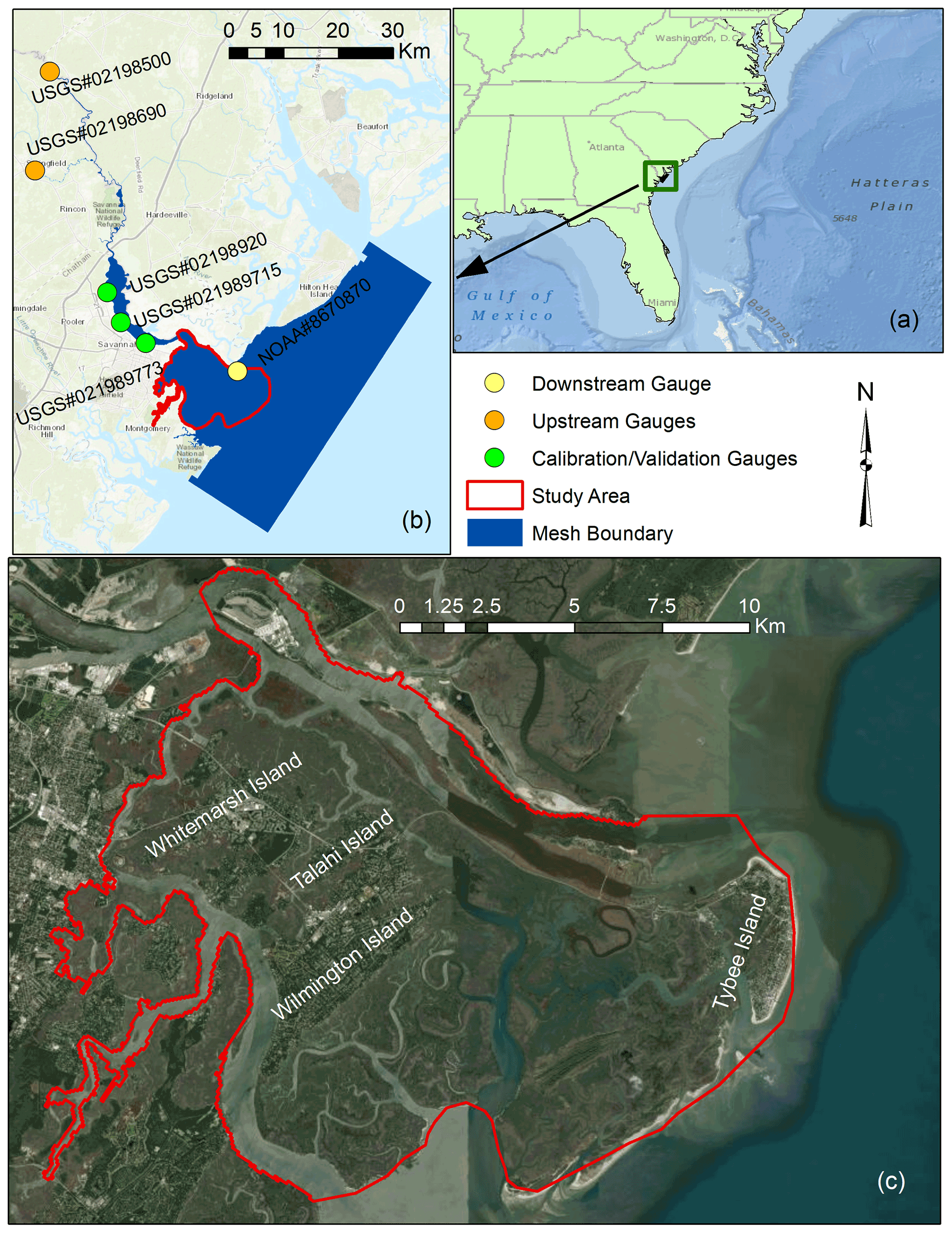
Figure 1Map of the study area and mesh boundary of the hydrodynamic model. (a) The geographic location of the study area in the southeast USA. (b) The mesh boundary used by the hydrodynamic model (blue) for flood inundation mapping as well as the location of upstream (orange), downstream (yellow), and calibration/validation (green) gauges, and (c) the boundary of Savannah wetlands used as the case study along with urbanized areas (Esri 2018).
We study the Savannah River delta located at the border of Georgia and South Carolina in the southeast United States (Fig. 1a). The Savannah River originates at the confluence of the Tugaloo and Seneca rivers and drains the lower Savannah watershed (HUC8_03060109) comprising an area of 2603.96 km2. The morphology of this region is relatively complex due to the existence of a braided river followed by a dense drainage network of interior rivers and tidal creeks. The average slope, length, and annual discharge of the Savannah River are 0.00011 m m−1, 505 km, and 320 m3 s−1, respectively (Carlston, 1969). Moreover, the river bathymetry was deepened to up to 12 m for increasing the capacity of cargo transportation (U.S. Army Corps of Engineers, 2017). This region is mostly characterized by its unique ecology, including vast wetlands and salt marsh ecosystems. We obtain detailed drainage network data including river streams, tidal channels, and creeks within wetland areas from the US National Wetlands Inventory (https://www.fws.gov/wetlands/data/Mapper.html, last access: 23 September 2021).
To simulate the flood hazard in this region, a mesh boundary encompassing the Savannah River delta, surrounding areas, and a portion of the Atlantic Ocean is generated (Fig. 1b). Two US Geological Survey (USGS) gauges, located at the Savannah River (nos. 02198500 and 02198690) and the Fort Pulaski station of the National Oceanic and Atmospheric Administration (NOAA) are used as upstream and downstream boundary conditions, respectively, of the hydrodynamic model. The Fort Pulaski station (NOAA – 8670870) provides an 85-year length of records (since 1935) that enables a proper characterization of coastal flooding for design levels at lower frequencies or relatively large return periods. We select this region as a test bed because of (1) frequent coastal flooding induced by large semidiurnal tidal amplitudes at the estuary mouth (Cowardin et al., 2013) and (2) exposure of more than 20 000 people settled in four developed areas, the Whitemarsh, Talahi, Wilmington, and Tybee islands located in this region (Fig. 1c).
The high-resolution DEM used as the base of our proposed hydrogeomorphic index is a 3 m light detection and ranging (lidar) that includes topographic and bathymetric (topobathymetric) data. This dataset has been developed by NOAA's National Centers for Environmental Information (NCEI) and is available at NOAA's Data Access Viewer repository (https://coast.noaa.gov/dataviewer/, last access: 23 September 2021). The topobathymetric data were further corrected for wetland elevation error using the DEM-correction tool developed by Muñoz et al. (2019) to minimize vertical bias errors commonly found in lidar-derived coastal DEMs (Alizad et al., 2018; Medeiros et al., 2015; Rogers et al., 2018). The vertical and horizontal accuracies of the DEM are 50 and 100 cm, respectively, and its vertical datum is the North American Vertical Datum 1988 (NAVD 88). Land cover maps are obtained from the 2016 National Land Cover Database (NLCD) available at https://www.mrlc.gov/ (last access: 23 September 2021). River discharge and WL records are obtained from the USGS (https://maps.waterdata.usgs.gov/mapper/index.html, last access: 23 September 2021) and NOAA (https://tidesandcurrents.noaa.gov/, last access: 23 September 2021), respectively. In addition, post-flood high-water marks (HWMs) of Hurricane Irma and Hurricane Matthew are obtained from the USGS Flood Event Viewer platform (https://stn.wim.usgs.gov/FEV/, last access: 23 September 2021). These high-water marks are used for calibration and validation of the Savannah model in Delft3D FM. Specifically, we used the 2021 Delft3D FM suite package to model the complex interactions between riverine, estuarine, and intertidal flat hydrodynamics. The suite package can provide detailed information on water level, flow rates, and velocity (Delft3D Flexible Mesh Suite, 2021).

Figure 2Flowchart of the proposed approach for generating hydrogeomorphic threshold operative curves. In Phase 1, the 2D hydrodynamic model is calibrated and generates the required reference maps for the next phase. In Phase 2, the reference maps are used in conjunction with the hydrogeomorphic index to generate the operative curves for fast and real-time coastal flood hazard assessment.
We propose a DEM-based LCFM approach for the rapid assessment of flood hazard areas in real time. The proposed approach consists of two phases (Fig. 2). In Phase 1, a 2D hydrodynamic model is calibrated based on observed WLs at USGS gauges and HWMs that were available during Hurricane Matthew in 2017. We then use the calibrated hydrodynamic model to generate a flood inundation map that serves as a reference map in the next phase. In addition, for flood frequency analyses, we perform a block maxima sampling approach to select the annual WL maxima at the Fort Pulaski station. The selected samples are then used to estimate WLs for six return periods of 10-, 50-, 100-, 200-, 500-, and 1000-year floods. Using these estimated WLs as the main boundary conditions of the hydrodynamic model, we also generate six flood inundation maps corresponding to these return periods. In Phase 2, we use a high-resolution DEM together with the drainage network data to calculate the hydrogeomorphic index. Subsequently, the flood inundation map generated for Hurricane Matthew in Phase 1 is used as a reference map to calibrate the hydrogeomorphic index. Then, the calibrated index uses the flood inundation maps provided for different return periods in Phase 1 to develop the operative curves. These curves form the basis for the rapid assessment of flood hazard areas for any upcoming coastal flood event in the future. To validate the effectiveness and reliability of the developed operative curves, we use them to identify hazard areas corresponding to Hurricane Irma, and then we compare their accuracy with the reference map provided by the hydrodynamic model for this flood event. In the following sections, we further explain the hydrodynamic model, flood frequency analysis, and hydrogeomorphic method.
3.1 Hydrodynamic model
3.1.1 Model setup
We use the 2019 Delft3D FM suite package (Delft3D Flexible Mesh Suite, 2019) to model the complex riverine, estuarine, and intertidal flat hydrodynamics in the Savannah River delta and wetland regions. The suite package has been used with satisfactory results in similar coastal studies characterized by vast wetland regions (Fagherazzi et al., 2014; Kumbier et al., 2018; Sullivan et al., 2019). Moreover, the model developed for the Savannah has been used in other studies to simulate extreme and non-extreme events including Hurricane Matthew, which hit the southeast Atlantic coast in October 2016 (Muñoz et al., 2021, 2020). The 2D hydrodynamic model comprises nearly 85 km of the Savannah River extending from the Fort Pulaski station (NOAA – 8670870) at the coast up to the Clyo station (USGS – 02198500) and covers an area of 1178 km2 approximately. The model consists of an unstructured triangular mesh to ensure a correct representation of geomorphological settings including sinuous and braided river waterways and relatively narrow tidal inlets. Furthermore, the mesh has a spatially varying cell size ranging from 1.5 m in the upstream riverine area, 10 m over wetland regions, 120 m along the coast, to up to 1.4 km over the Atlantic Ocean (Fig. 1b).
3.1.2 Model calibration
For calibration purposes, the model was forced with time series of river flow obtained from the Clyo station as an upstream boundary condition (BC); the coastal WL from the Fort Pulaski station as a downstream BC; and with spatially varying Manning's roughness values (n) classified into open-water, wetland, urban, and riverine areas. The optimal (or calibrated) set of n values was inferred from 200 model simulations of Hurricane Matthew as this event reported the highest peak WL at the Fort Pulaski station since the year 1935 (2.59 m with respect to NAVD 88). Each simulation was conducted in a high-performance computing system and included a 1-month warm-up period and a unique set of n values for each land cover generated with the Latin hypercube sampling (LHS) technique (Helton and Davis, 2003). The advantage of LHS over traditional Monte Carlo approaches is that the former results in a denser stratification over the range of each sampled parameter and is therefore superior to random sampling. LHS leads to more stable results that are closer to the true probability density function of the parameter and has been used in similar studies (Jafarzadegan et al., 2021; Muñoz et al., 2022). The range of n values was derived from pertinent literature and included hydrodynamic modeling and open-channel flow studies (Arcement and Schneider, 1989; Chow Ven, 1959; Liu et al., 2019). The set of values achieving both the lowest root mean square error (RMSE) and the highest Kling–Gupta efficiency (KGE) around the peak WL (e.g., 7 d window) was selected as the optimal one and further used for coastal flood simulations. KGE is a robust evaluation metric that accounts for correlation, bias, and the ratio of variances and can take values between −∞ and 1 (Gupta et al., 2009). An efficiency of 1 indicates a perfect match between model simulations and observations. In addition to those metrics, we evaluate the model's performance using the Nash–Sutcliffe efficiency (NSE) and mean absolute bias (MAB). NSE measures the relative magnitude of the error variance of model simulations compared to the variance of observational data (Nash and Sutcliffe, 1970). NSE ranges between −∞ and 1, where an efficiency of 1 indicates a perfect match. MAB quantifies the bias of model simulations with respect to observational data. MAB of 0 suggests an absence of bias in the simulation. The calibrated n values used in the Savannah model are open-water (n=0.027), wetland (n=0.221), urban (n=0.03), and downstream and upstream riverine (n=0.037 and n=0.086, respectively) areas.
3.2 Flood frequency analysis
Preliminary model simulations indicate a negligible influence of river flow on coastal wetland inundation as compared to storm surge on Wassaw Sound and Wilmington and Tybee islands (Fig. 1c). This can be explained by the proximity of the islands to the Atlantic Ocean as well as freshwater runoff regulation and flood controls by three large dams located upstream of the Clyo station (USGS – 02198500), namely J. Strom Thurmond, Richard B. Russell, and Hartwell (Zurqani et al., 2018). In addition, bivariate statistical analysis via copulas suggests no significant correlation between river flow at the Clyo station (USGS – 02198500) and coastal water levels at the Fort Pulaski station (NOAA – 8670870). The latter was also reported in Ghanbari et al. (2021) and Muñoz et al. (2020). Furthermore, our analysis demonstrated that high river flow does not affect the inundation area in wetlands. This indicates that flood inundation is highly dominated by coastal forcing as tides propagate into the Savannah River and lead to flow reversal at upstream gauge stations (see Fig. 1 below). The high proximity of wetlands to the Atlantic Ocean shows that the transitional zone, i.e., the area affected by both coastal and inland drivers, is located upstream of the Port Wentworth station (USGS – 02198920) where the Savannah River trifurcates into the Back River, Middle River, and Front River. Considering the dominant role of the seawater level in coastal flooding as well as the negligible effect of river discharge on wetland inundation from the previous analyses, we can justify the proposed univariate flood frequency analysis. We, therefore, conduct a univariate flood frequency analysis based on annual block maxima sampling of WLs observed at the Fort Pulaski station. We use the “allfitdist” tool in MATLAB to find the best parametric probability distribution fit to the data, based on the maximum likelihood, Bayesian information criterion (BIC), or Akaike information criterion (AIK).
3.3 Hydrogeomorphic index
Among different hydrogeomorphic features used for flood hazard mapping, HAND (sometimes also referred to as feature H) has been widely used as one of the best indicators of floodplains. However, due to the weakness of this feature for proper characterization of floodplains in flat regions and coastal areas, here we develop a composite hydrogeomorphic index that considers H as well as the distance to the nearest drainage (D). Although the overall performance of feature D is less than H in most case studies (Degiorgis et al., 2012; Manfreda et al., 2015a; Samela et al., 2016), feature D can be a better descriptor of floodplains in highly flat regions according to the study conducted by Samela et al. (2017). In another study, Gharari et al. (2011) proposed a composite index by multiplying both features H and D and demonstrated that H is a better feature compared to the case that both features are used for landscape classification. The main drawback of their proposed index was that they used the same weights for both features, which results in degrading the classification performance. To overcome the limitation of the proposed index and to consider the key role of feature D in flat areas, we maintain feature D in our composite index and add different weights to H and D using Eq. (1) as follows:
where .
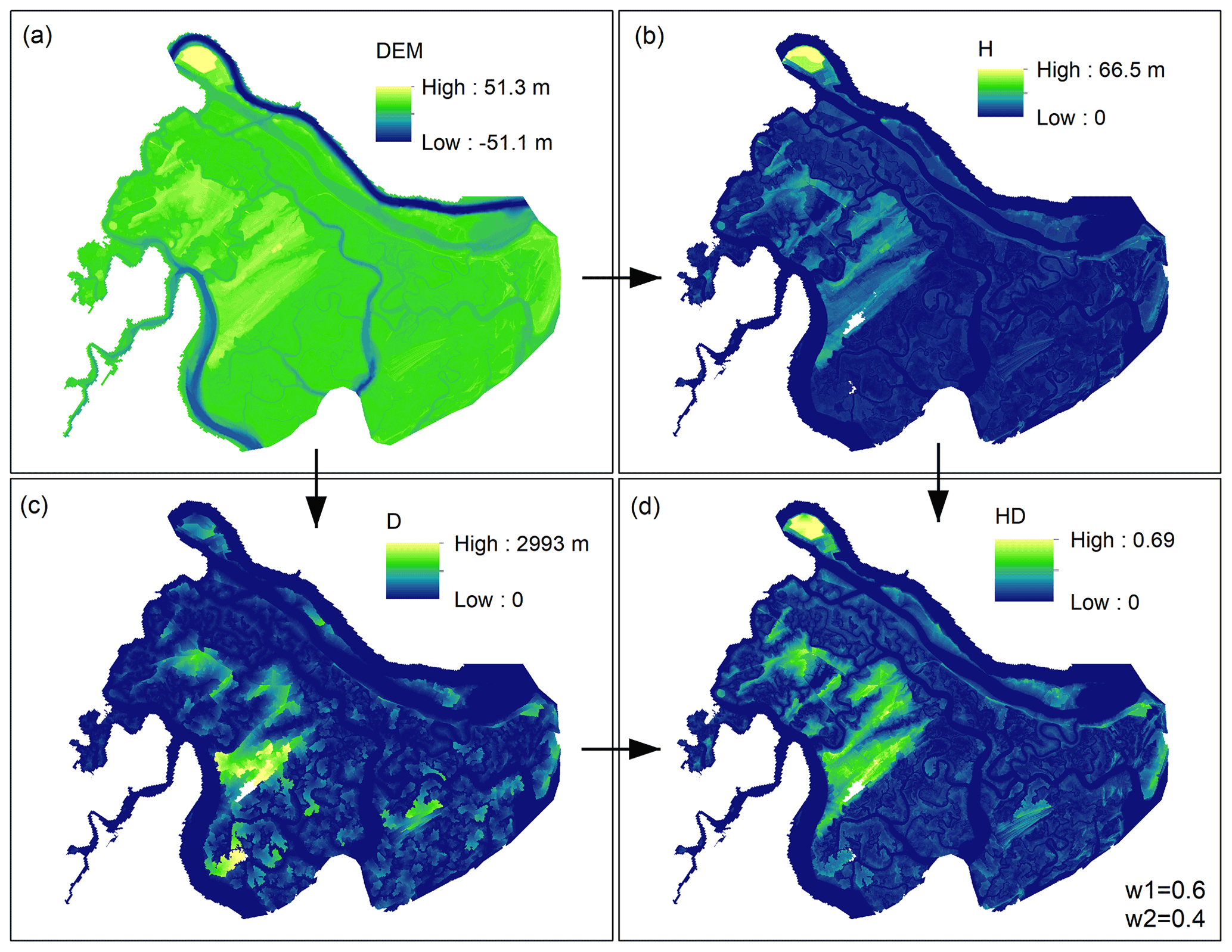
Figure 3The required steps for calculating the proposed hydrogeomorphic index. A high-resolution coastal DEM (3 m) is used as the source data (a) to generate the height above nearest drainage (H) and the distance to the nearest drainage (D) (b and c, respectively). Using Eq. (1), the normalized features H and D are multiplied with different weights to generate the IHD index (d).
In Eq. (1), Hmax and Dmax denote the maximum value of raster H and D used for normalizing the hydrogeomorphic index, whereas w1 and w2 refer to the weights of feature H and D, respectively. The conditional equation of helps lower the computational burden of the calibration procedure by reducing the number of unknown parameters from two to one. Figure 3 illustrates an example of calculating the IHD index with a given set of weights (w1=0.6 and w2=0.4) for the study area. Using a high-resolution coastal DEM (Fig. 3a), raster H and D are calculated (Fig. 3b and c). Considering a DEM with N cells, the main step is to find a coordinate matrix that indicates the location of the nearest stream cell to each grid cell. Knowing this matrix and the number of cells required to cross the nearest stream cell, the feature D is calculated. The coordinate matrix can also be used in conjunction with the DEM to calculate the feature H. To calculate the IHD index, the weights in Eq. (1) are calibrated using a reference flood hazard map obtained from hydrodynamic simulation (e.g., Hurricane Matthew). We tested 100 combinations of weight parameters (w1 and ), derived from random generation of 100 w1 values in the range of 0–1, to find the importance of features H and D, and then finalized the IHD index with known parameters for future flood hazard mapping. We further validated the weight parameters through the simulations of Hurricane Irma.
3.4 Binary classifiers for flood hazard mapping
Considering the study area a grid of cells, a binary classifier assigns a value of zero or 1 to each cell and generates a map of two different classes. In flood hazard mapping, the common approach is to define a threshold on a hydrogeomorphic index (e.g., IHD) and use the following if-then-else rule for the classification:
where f(i) and denote the label of flood hazard map and the proposed hydrogeomorphic index value at cell i, respectively, and TH denotes the threshold of the hydrogeomorphic classifier that should be calibrated. The flood hazard map generated with the binary classifier is compared with a binary reference hazard map, and the rate of true positives (rtp), rate of false positives (rfp), and error are calculated as follows (Jafarzadegan and Merwade, 2017):
In binary classification, positive and negative refer to a value of 1 and zero, respectively. True positive instances are those positive cells that are correctly predicted by the classifier, and false positive instances represent those negative cells that are wrongly classified as positive. The error, reflecting all cells that are wrongly predicted by the classifier, is a commonly used measure for validating the performance of binary classifiers for flood hazard mapping. Another useful performance measure to validate the binary classifier is the area under the curve (AUC) of the receiver operating characteristic (ROC) graph proposed by Fawcett (2006).
To calibrate the binary classifier, we minimize the error while searching for the optimum TH value. This means we use 100 TH values uniformly picked from the range of and . For each TH value, we use Eq. (2) to generate a binary hazard map and then compare this map with the reference map by calculating the error from Eqs. (3)–(5). In this optimization problem, the reference flood hazard map used for calculating the error is the key input that should be further described. The flood inundation maps generated by the hydrodynamic model indicate WLs at different cells in different time steps and should be converted to a single binary map. A common approach used for inland floods is to find the maximum inundation area over the entire flooding period and then assign all cells with zero WL to “dry” or “non-flooded” and other cells with positive values as “wet” or “flooded”. In delta estuaries and coastal regions near the ocean, however, almost all cells can be flooded with small WL values. Therefore, after finding the maximum inundation over the flooding period, we use another set of binary labels as “low hazard” vs. “high hazard” and define the hazard depth cutoff (HDC) as a threshold used to convert a continuous map of WL to a binary map with only two labels. Depending on the HDC used for distinguishing low- from high-hazard regions, the reference flood map is changed, which results in a different calibrated TH. In addition to HDC, the intensity of the flood event shown with the return period also changes the reference flood hazard map. Therefore, the calibrated parameter TH is a function of both HDC and T, and the main goal of this study is to provide operative curves showing the variation in TH with these two factors. We run the hydrodynamic model for six different return periods of 10-, 50-, 100-, 200-, 500-, and 1000-year events and then convert the WL maps to binary maps using 21 HDC values resulting from 0.1 increments in the range of 0–2 m. The binary classification and calibration of TH are performed for different reference maps generated from various combinations of T and HDC.
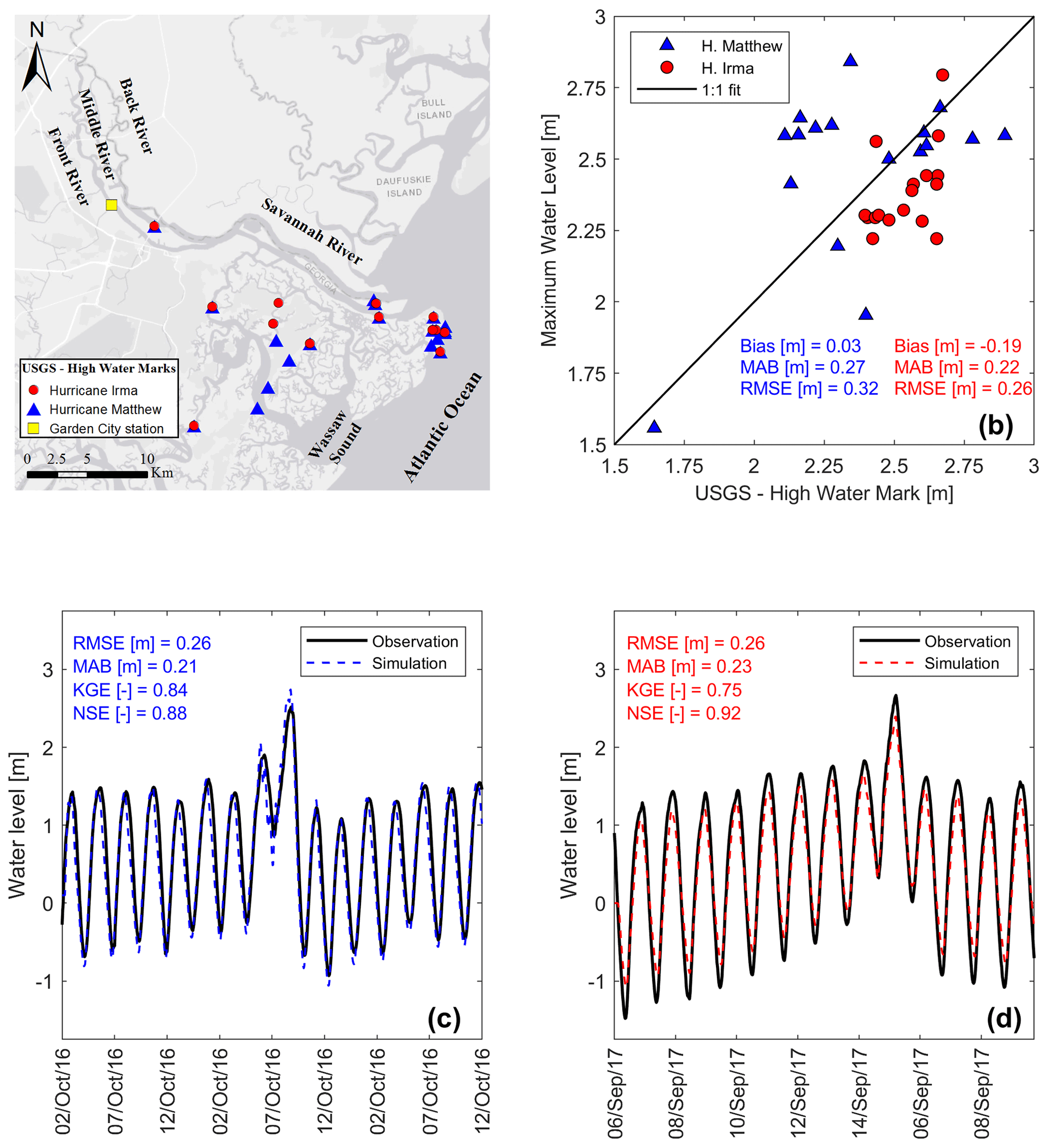
Figure 4Calibration and validation of the Savannah Delft3D FM model. (a) Location of high-water marks (HWMs) in the Savannah River delta for Hurricane Matthew (blue triangles) and Hurricane Irma (red circles). (b) Comparison between simulated maximum water levels (WLs) and HWMs in the Savannah. (c, d) Time series of simulated and observed WLs at the Garden City station for Hurricane Matthew and Hurricane Irma, respectively.
A comprehensive calibration and validation of the Savannah River model is shown in Fig. 4. This step is crucial to ensure that the flood hazard maps provided by the model are reliable enough to be used as the reference of the hydrogeomorphic method. We assess the performance of the model by first comparing simulated and observed WLs at three USGS stations along the Savannah River (Fig. 1b, green circles). For convenience, we only present simulated and observed WLs of Hurricane Matthew and Hurricane Irma at Garden City (Fig. 4c and d, respectively) located ∼ 29.5 km from the river mouth (Fig. 4a, yellow square). The results of the remaining stations are included in Fig. S1 in the Supplement. RMSE and MAB remain below 30 and 25 cm, whereas KGE and NSE achieve values above 0.75 and 0.85, respectively, for the two hurricane events, which is reflective of satisfactory model performance. Overall, the magnitude and timing of the highest peak WL observed during the hurricanes are well captured by the Savannah River model. To further evaluate the model performance in coastal flood propagation analysis, we compare maximum WLs resulting from model simulations with the USGS HWMs collected in urban and surrounding wetland areas (Fig. 4b). The 1:1 line represents a perfect fit between simulated and observed maximum WLs and helps visualize overestimation (above the 1:1 line) and underestimation of the model. Similarly, the evaluation metrics indicate a satisfactory performance of the model with a slight over- and underestimation during Hurricane Matthew and Hurricane Irma. Moreover, the model achieves a relatively small RMSE (< 35 cm).
To generate boundary conditions for coastal flood modeling simulations associated with the proposed return periods, we perform flood frequency analysis of coastal WL at the Fort Pulaski station (in Fig. 5) located at the mouth of the Savannah River (Fig. 1b, yellow circle). In this study, we select the generalized extreme value (GEV) because of its smallest estimated BIC compared to other parametric distributions available with the MATLAB allfitdist tool. In addition, we show the 95 % confidence bounds of the GEV distribution and fit a non-parametric Weibull distribution to the data for comparison purposes. Hereinafter, we will use the GEV distribution to estimate WLs for 10-, 50-, 100-, 200-, 500-, and 1000-year return periods.

Figure 5Return water levels (WLs) for the Fort Pulaski station in the Savannah, GA (NOAA – 8670870). Plotting positions (black crosses) are derived from the Weibull formula based on annual block maxima time series (AMAX) and comparable to the generalized extreme value (GEV) distribution (blue circles). The 95 % confidence intervals (CIs) for the distribution parameters of the GEV distribution are shown with a blue-shaded band.
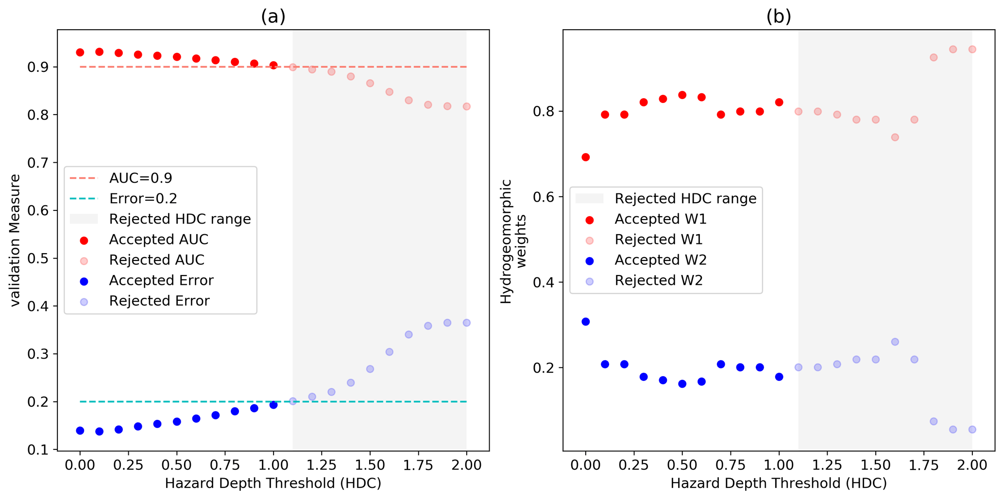
Figure 6Calibration of the IHD index for Hurricane Matthew. (a) The variation in performance measures AUC (red) and error (blue) for different hazard depth cutoff (HDC) values and (b) the optimum weights of the IHD index for different HDC values. The dashed lines show the maximum error (0.2) and minimum AUC (0.9) that are acceptable for flood hazard mapping. Using these criteria, the gray regions show that the hydrogeomorphic model cannot provide acceptable results for HDC values higher than 1.1 m.
After calibrating the Delft3D FM model, we generate daily flood inundation maps for Hurricane Matthew, determine the maximum flood extent among all days, and then use an HDC to convert the maximum inundation map to a binary map of low- and high-hazard classes. Using 21 different HDCs ranging from 0 to 2 m, we perform 21 calibrations corresponding to a given reference flood hazard map generated from a specific HDC value. Figure 6a shows the error and AUC of calibration corresponding to different HDC values. As can be seen, increasing the HDC decreases the accuracy of the hydrogeomorphic method for flood hazard mapping. Looking into the errors and AUC values reported in the literature of binary flood hazard mapping studies, we consider an error of 0.2 and an AUC of 0.9 (dashed lines) as the limits for distinguishing acceptable models from unacceptable ones. The gray region indicates the rejected HDC values above 1.1 m that result in unacceptable accuracy (e.g., error > 0.2 or AUC < 0.9). Figure 6b indicates the optimum weights calculated from the calibration of the hydrogeomorphic method corresponding to different HDC values. The higher value of w1 compared to w2 demonstrates that feature H is a more important factor than feature D in representing the flood hazard areas, and a combination of both features is the best indicator of floodplains compared to using each feature individually (w1=0 or w2=0). Figure 6b also shows that for the HDC = 0 (wet vs. dry classification), feature D shows the highest contribution (30 %), while using the high HDC value of 2 m decreases the contribution of this feature to almost zero.
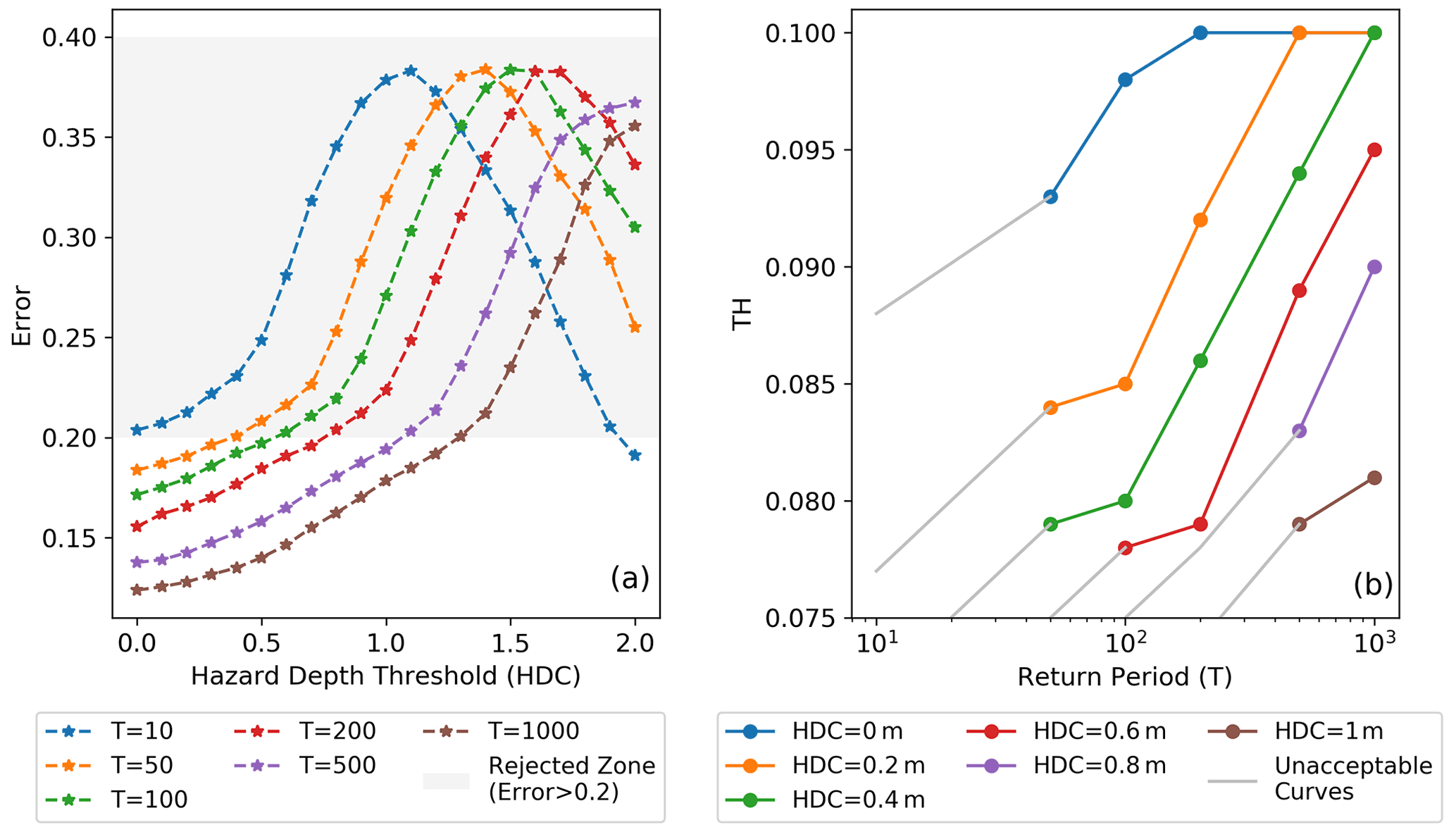
Figure 7(a) The errors in flood hazard maps generated by the calibrated hydrogeomorphic method for different return period flood events and hazard depth cutoff (HDC) values. (b) The hydrogeomorphic threshold operative curves provided for different HDC values. These operative curves are the major tool for fast flood hazard mapping as, depending on the return period of a future flood event and the HDC value chosen by the decision maker, the operative curves estimate the hydrogeomorphic threshold. Knowing this threshold, the flood hazard map will be generated in a few minutes.
To generate the operative curves for future flood events, we design 36 scenarios that include six HDCs (0, 0.2, 0.4, 0.6, 0.8, 1 m) from the acceptable range of 0–1 m for six different reference hazard maps, provided by the Delft3D FM model for return periods of 10, 50, 100, 200, 500, and 1000 years. Each scenario provides a reference hazard map, so binary classification is performed to estimate TH corresponding to each scenario. Figure 7a indicates the error curves for different return period events. For low HDCs, increasing the magnitude of the flood (higher return period) results in more accuracy of the hydrogeomorphic method. This pattern is reversed for high HDCs where a flood event with a 10-year return period provides the highest accuracy. In general, the gray region shows that for high HDCs, the performance of the hydrogeomorphic method is poor for almost all return periods, while for low HDCs, all flood events can be accurately used for flood hazard mapping. Figure 7b illustrates the hydrogeomorphic threshold operative curves for future flood hazard mapping. The TH on the y axis is the key value that can be estimated for each combination of HDC and return period. Knowing this threshold, Eq. (2) can be used to rapidly estimate the hazard areas for future floods. As expected, a higher magnitude of flood needs a higher hydrogeomorphic threshold, while increasing HDC (smaller high-hazard areas) requires a smaller threshold for binary classification. The gray parts of the curves refer to those scenarios that have unacceptable accuracy, so it is recommended to not use HDCs corresponding to these parts.
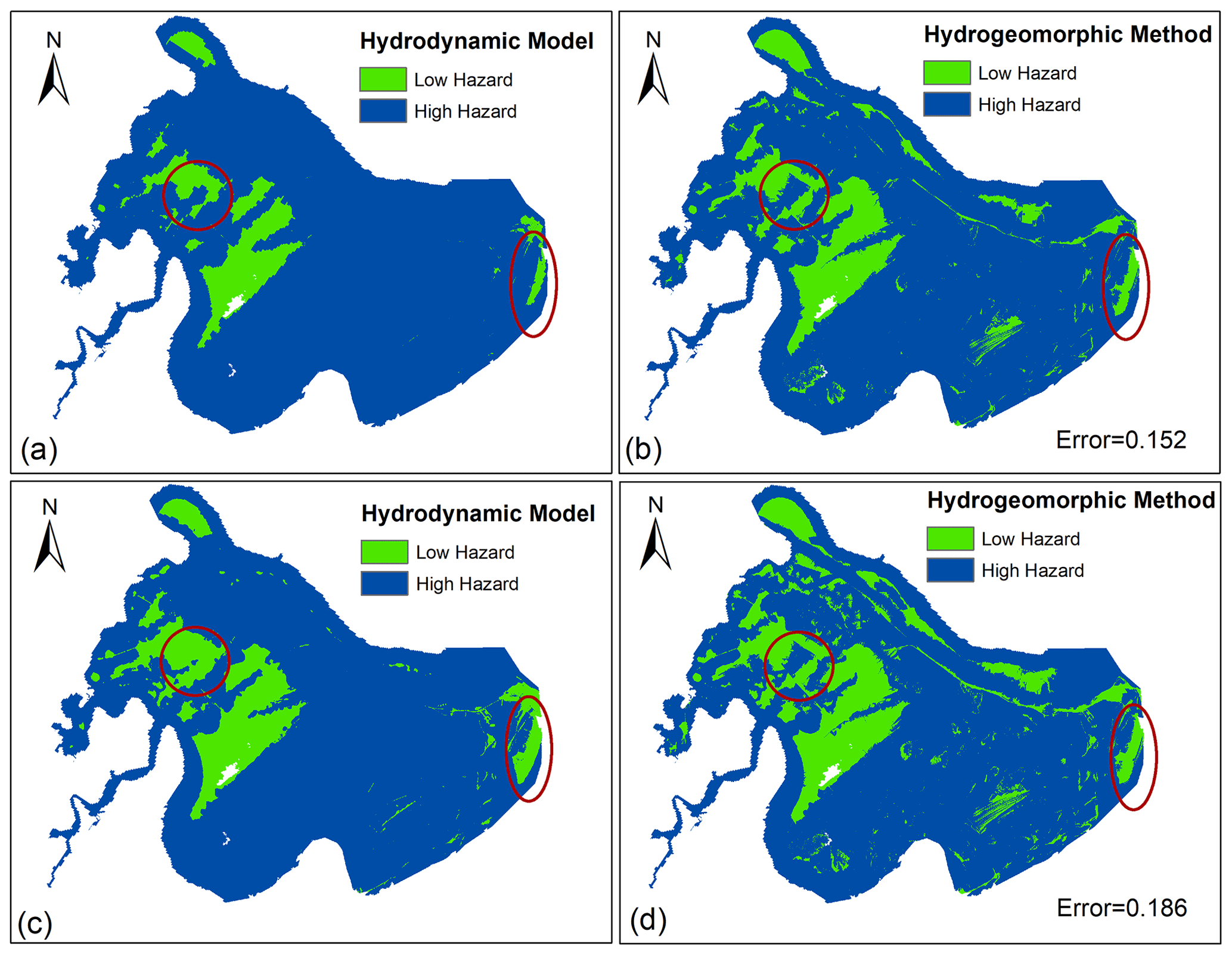
Figure 8Validation results for Hurricane Irma showing a side-by-side comparison of flood hazard maps generated by the hydrodynamic model and hydrogeomorphic method for two different hazard depth cutoffs (HDCs): HDC = 0 (a, b) and HDC = 0.6 m (c, d). To generate the flood hazard maps by the hydrogeomorphic method, the operative curves estimate two hydrogeomorphic thresholds of 0.1 and 0.08 for HDC = 0 m and HDC = 0.6 m, respectively, and the return period of Hurricane Irma is estimated as a 223-year flood event.
Finally, we evaluate the accuracy and effectiveness of the proposed operative curves by validating their performance in generating flood hazard areas during Hurricane Irma. The maximum WL during this flood event was 2.49 m, which corresponds to a 223-year flood event according to our flood frequency analysis (e.g., GEV distribution). For two HDCs of 0 and 0.6 m, the operative curves suggest the hydrogeomorphic thresholds of 0.1 and 0.08, respectively. Using these thresholds and Eq. (2), the flood hazard maps corresponding to Hurricane Irma can be generated. Figure 8 indicates a side-by-side comparison of flood hazard maps generated by the Delft3D FM model (Fig. 8a and c) and the hydrogeomorphic threshold operative curves (Fig. 8b and d) for two different HDCs of 0 (Fig. 8a and b) and 0.6 m (Fig. 8c and d). For both HDCs, errors (0.152 and 0.186) are less than a 0.2 limit used for reliable flood hazard mapping. The main discrepancies are some noisy, scattered low-hazard areas located in the east and southeast of the study area. These areas can reflect the flooded surface depressions (sinks) resulting from the pluvial impacts of extreme precipitation. Hydrodynamic models simulate the fluvial and coastal processes that occur adjacently to rivers and oceans while disregarding the pluvial impacts. The red circle in the left part of the panels shows a region that the hydrogeomorphic method cannot properly simulate, especially for higher HDCs. This can be due to the inability of the hydrogeomorphic method to properly simulate physical processes. On the other hand, the red ellipse at the right side of the panels illustrates an urbanized region where the hydrogeomorphic method properly classifies the area compared to the reference map. Overall, the high overlap of the flood hazard maps provided by the hydrogeomorphic method with the reference maps provided by the hydrodynamic model (error < 0.2) illustrates the reliability and effectiveness of the proposed hydrogeomorphic method for flood hazard mapping. Besides, the high efficiency of this approach for rapid estimation of flood hazard maps (order of minutes) compared to the long computational time required for detailed hydrodynamic modeling (order of hours) suggests the proposed hydrogeomorphic method as an alternative for efficient flood hazard mapping during emergencies.
This study develops hydrogeomorphic threshold operative curves for rapid estimation of hazardous areas during emergencies of future coastal floods in deltas and estuaries. The low errors (< 0.2) of estimated hazard maps for Hurricane Irma generated by the proposed approach compared to the reference hydrodynamic model results demonstrate the high accuracy of the proposed operative curves for future flood events in this region. According to studies conducted on the binary classification of hydrogeomorphic features in the literature, the errors in the best classifiers were mostly in the range of 0.2–0.3 for inland floods (Degiorgis et al., 2012; Manfreda et al., 2014). Therefore, given the higher complexity of the terrain and drainage network in deltas, predicting the hazard maps with errors less than 0.2 (e.g., error of 0.152 for HDC = 0) is a promising achievement. The potential reasons explaining the high accuracy of the proposed binary classifier for wetlands include the high-resolution DEM used for mapping (∼ 3 m) and the incorporation of bathymetry into the DEM. In addition, the flexible structure of the proposed hydrogeomorphic index, with two varying weights of H and D features, allows for calibrating the index with the optimum contribution of each feature, which in return results in the highest accuracy.
The proposed hydrogeomorphic index (IHD) is the primary data for flood hazard mapping in this study. Thus, the quality of two main inputs of this index, namely the DEM and stream network used to calculate features H and D, play a vital role in the overall accuracy of the proposed approach. To obtain maximum accuracy, here we used the best available DEM with the finest spatial resolution of 3 m that includes the bathymetry data. However, considering the limited access to such high-quality DEMs in many areas of the world, it is recommended to evaluate the sensitivity of the proposed approach to lower-quality DEMs (e.g., 30 and 90 m DEMs without bathymetry information) in future studies. Another piece of research can investigate the sensitivity of the proposed approach to the density of the drainage network used for calculating the IHD index.
Unlike past studies that used binary classifiers for detecting hazard areas corresponding to past floods or generated static maps for a specific return period (Degiorgis et al., 2012; Jafarzadegan et al., 2018; Manfreda et al., 2015b; Samela et al., 2017), here we propose the hydrogeomorphic threshold operative curves for real-time flood hazard mapping. Considering the rapid occurrence of hurricane-induced flooding in deltas and estuaries, these curves can be highly beneficial for emergency responders to provide a preliminary estimation of hazard areas for an upcoming flood in these regions and to design the appropriate evacuation strategies. In addition, the proposed operative curves demonstrate the hydrogeomorphic threshold variations with HDCs. This feature of the operative curves gives additional flexibility to decision makers for estimating the hazard maps based on the HDC that is considered given the momentary safety issues. For example, identifying the hazard map based on HDC < 0.3 is useful for checking the operability and accessibility of essential facilities and infrastructure, while a hazard map corresponding to HDC = 1 indicates those areas that experience high WLs above 1 m as hazardous areas, with greater potential for casualties and significant structural damage. Overall, the hydrogeomorphic threshold operative curves are a function of both the return period (flood severity) and the HDC (a decision-making option that controls the definition of high hazard). Using a similar approach, future studies can provide these curves for inland floods as well. In addition, due to the practical benefits of these curves for efficient coastal flood hazard assessment, the hydrogeomorphic threshold operative curves can be extended to other deltas and estuaries that experience frequent flooding across the USA (e.g., Mississippi – Louisiana (LA), Galveston Bay – Texas (TX), Delaware Bay – Delaware (DE), Chesapeake Bay – Virginia (VA)) and the world (e.g., Yangtze – China, Brahmaputra – Bangladesh). To implement this approach, first, a hydrodynamic model should be set up for the new study area and generate reference inundation maps for different return periods. Access to observed water level data (gauges or HWMs) and flood extent maps from past floods is required to properly calibrate the hydrodynamic model. Then the IHD index calculated from a DEM is utilized together with the reference maps to provide the hydrogeomorphic threshold operative curves for future floods.
The reference maps used for training the binary classifier are key components for generating reliable results. Since these reference maps are the outcomes of hydrodynamic modeling, they are prone to uncertainties stemming from unrealistic parametrization, imperfect model structure, and erroneous forcing. The design floods used as boundary conditions of the hydrodynamic model are estimated from flood frequency analysis that is prone to uncertainty as well. Here, we used a bivariate approach that estimates the design flood based on the water level data. A more comprehensive flood frequency analysis that accounts for other flood attributes, such as volume, spatial dependencies, or nonstationarity, can improve the reliability of flood frequency analysis in future studies (Brunner et al., 2016; Yan and Moradkhani, 2015; Bracken et al., 2018). With access to less than 100 years of data for flood frequency analysis, the extreme return levels (i.e., 500- and 1000-year floods) pose high uncertainties due to the extrapolation of annual maxima data. This should warn decision makers to be more cautious about using operative curves for extreme flood events. For future studies, the uncertainty bounds of flood frequency analysis (especially extrapolations for extreme cases) can be considered in the modeling. In a real-time scenario, the forecasted WL used for flood frequency analysis is also prone to uncertainties originating from imperfect forecasting methods and nonstationary climate data. In addition, the uncertainty in model parametrization can be accounted for by running the hydrodynamic model for different combinations of optimum parameters. Model structure uncertainty can be also considered by using different hydrodynamic models and combining the results. Finally, probabilistic reference maps together with uncertainties involved in WL forecasting and flood frequency analysis can be integrated to develop probabilistic hydrogeomorphic threshold operative curves in future studies. This is in line with the report provided for the NOAA National Weather Service (NWS), showing the NWS stakeholders' preference for utilizing probabilistic storm surge inundation maps (NWS (National Weather Service), OAR (Oceanic and Atmospheric Research), and Eastern Research Group, Inc., 2013).
Operationally, the Sea, Lake, and Overland Surges from Hurricanes (SLOSH) model (Jelesnianski et al., 1984) is the storm surge model currently used by the NWS to perform storm surge forecasting and create probabilistic flood inundation maps for real-time tropical storms (Sea, Lake, and Overland Surges from Hurricanes (SLOSH), 2022). The feature of SLOSH that makes it the preferred model of the NWS for storm surge forecasting and mapping is the model's computational efficiency that allows the model to be run as an ensemble (Forbes et al., 2014). However, SLOSH is just one of several modeling options for storm surge modeling and mapping, each possessing strengths and weaknesses associated with their simulations. The inclusion of additional models that can create flood maps of storm surges for a given event should provide an enhanced understanding of the uncertainty in inundation at a given location (Teng et al., 2015). However, the higher computational burden of alternative models, such as Delft3D FM, tends to preclude their use in real-time operations and, certainly, their use in generating an ensemble necessary for probabilistic flood maps. The methodology we propose in this paper may offer the NWS and other agencies a means to utilize alternatives to SLOSH for flood inundation mapping and probabilistic flood inundation mapping on US coastlines. Models such as Delft3D FM can generate reference maps to train the binary classifier and build the probabilistic operating curves. The probabilistic operative curves would account for the major source of uncertainties and provide a computationally efficient and reliable decision-making tool for coastal planners and floodplain managers. The operative hydrogeomorphic threshold classifiers proposed for real-time coastal flood hazard mapping can be used as an alternative tool for the rapid estimation of hazardous areas during real-time flood events. In an operational mode, the water level or meteorological forecasts can be used to estimate the return period of an upcoming coastal flood event, and the methodology here can utilize this as an input to perform LCFM flood inundation mapping both deterministically and probabilistically.
Another LCFM approach is to train machine learning algorithms on reference inundation maps provided by well-calibrated hydrodynamic models (Bass and Bedient, 2018). A benchmark study that compares the performance (accuracy and efficiency) of two LCFM methods, including our proposed DEM-based hydrogeomorphic classifier and the surrogate machine-learning-based algorithm and the SLOSH model, is highly recommended for future studies.
In this study, we proposed binary classifiers for efficient flood hazard mapping in deltas and estuaries. HAND, typically used for modeling inland floods, is modified for flat regions along the coastline, and a new hydrogeomorphic index (IHD) that comprises both HAND and the distance to the nearest drainage was developed. The DEM used as the base of these binary classifiers is a 3 m lidar that includes bathymetric information. This is another improvement compared to previous DEM-based classifiers that commonly used 10–30 m DEMs without bathymetric data. The IHD index has two unknown weights that show the contribution of both HAND and feature D. We simulated Hurricane Matthew with the Delft3D FM model and used the results as a reference flood hazard map to calibrate the IHD index. Using Delft3D FM again, we generated six flood hazard maps corresponding to different return periods and employed these maps as a reference to generate the hydrogeomorphic threshold operative curves. Finally, we validated the proposed operative curves for reliable and efficient flood hazard mapping by comparing the flood hazard maps generated for Hurricane Irma with the proposed curves and the Delft3D FM model. The high accuracy of validation results (< 0.2 error) together with the computational efficiency of this approach for real-time flood hazard mapping suggests the proposed operative curves as a practical decision-making tool for on-time and reliable estimation of hazard areas in estuaries.
All the data used in this study, including the gauge streamflow and water stage data, are publicly available from the USGS and NOAA websites. The high-water marks provided for Hurricane Irma and Hurricane Matthew are available from the USGS Flood Event Viewer platform.
The supplement related to this article is available online at: https://doi.org/10.5194/nhess-22-1419-2022-supplement.
KJ and HamiM conceptualized the study. KJ designed the whole framework and implemented the hydrogeomorphic methodology. DFM implemented the hydrodynamic model. KJ and DFM wrote the first draft of the manuscript. HamiM, HameM, JLG, and GS provided comments and edited the manuscript.
The contact author has declared that neither they nor their co-authors have any competing interests.
Publisher's note: Copernicus Publications remains neutral with regard to jurisdictional claims in published maps and institutional affiliations.
This work was financially supported by USACE award no. A20-0545-001. We would like to thank the anonymous reviewers for their constructive comments on the original version of the manuscript.
This research has been supported by the U.S. Army Corps of Engineers (grant no. A20-0545-001).
This paper was edited by Mauricio Gonzalez and reviewed by two anonymous referees.
Afshari, S., Tavakoly, A. A., Rajib, M. A., Zheng, X., Follum, M. L., Omranian, E., and Fekete, B. M.: Comparison of new generation low-complexity flood inundation mapping tools with a hydrodynamic model, J. Hydrol., 556, 539–556, https://doi.org/10.1016/j.jhydrol.2017.11.036, 2018.
Alizad, K., Hagen, S. C., Medeiros, S. C., Bilskie, M. V., Morris, J. T., Balthis, L., and Buckel, C. A.: Dynamic responses and implications to coastal wetlands and the surrounding regions under sea level rise, PLOS ONE, 13, e0205176, https://doi.org/10.1371/journal.pone.0205176, 2018.
Arcement, G. J. and Schneider, V. R.: Guide for selecting Manning's roughness coefficients for natural channels and flood plains, U.S. Geological Survey, https://ton.sdsu.edu/usgs_report_2339.pdf (last access: 23 September 2021), 1989.
Barbier, E. B.: Chapter 27 – The Value of Coastal Wetland Ecosystem Services, in: Coastal Wetlands, edited by: Perillo, G. M. E., Wolanski, E., Cahoon, D. R., and Hopkinson, C. S., Elsevier, 947–964, https://doi.org/10.1016/B978-0-444-63893-9.00027-7, 2019.
Bass, B. and Bedient, P.: Surrogate modeling of joint flood risk across coastal watersheds, J. Hydrol., 558, 159–173, https://doi.org/10.1016/j.jhydrol.2018.01.014, 2018.
Bates, P. D., Horritt, M. S., and Fewtrell, T. J.: A simple inertial formulation of the shallow water equations for efficient two-dimensional flood inundation modelling, J. Hydrol., 387, 33–45, https://doi.org/10.1016/j.jhydrol.2010.03.027, 2010.
Bates, P. D., Quinn, N., Sampson, C., Smith, A., Wing, O., Sosa, J., Savage, J., Olcese, G., Neal, J., Schumann, G., Giustarini, L., Coxon, G., Porter, J. R., Amodeo, M. F., Chu, Z., Lewis-Gruss, S., Freeman, N. B., Houser, T., Delgado, M., Hamidi, A., Bolliger, I., McCusker, K. E., Emanuel, K., Ferreira, C. M., Khalid, A., Haigh, I. D., Couasnon, A., Kopp, R. E., Hsiang, S., and Krajewski, W. F.: Combined Modeling of US Fluvial, Pluvial, and Coastal Flood Hazard Under Current and Future Climates, Water Resour. Res., 57, e2020WR028673, https://doi.org/10.1029/2020WR028673, 2021.
Bracken, C., Holman, K. D., Rajagopalan, B., and Moradkhani, H.: A Bayesian hierarchical approach to multivariate nonstationary hydrologic frequency analysis, Water Resour. Res., 54, 243–255, 2018.
Brunner, M. I., Seibert, J., and Favre, A.-C.: Bivariate return periods and their importance for flood peak and volume estimation, WIREs Water, 3, 819–833, https://doi.org/10.1002/wat2.1173, 2016.
Carlston, C. W.: Longitudinal Slope Characteristics of Rivers of the Midcontinent and the Atlantic East Gulf Slopes, Int. Assoc. Sci. Hydrol. Bull., 14, 21–31, https://doi.org/10.1080/02626666909493751, 1969.
Chow Ven, T.: Open channel hydraulics, McGraw-Hill Kogakusha, Tokyo, 680 pp., 1959.
Cowardin, L. M., Carter, V., Golet, F. C., and Laroe, E. T.: Classification of Wetlands and Deepwater Habitats of the United States, in: Water Encyclopedia, edited by: Lehr, J. H. and Keeley, J., John Wiley & Sons, Inc., Hoboken, NJ, USA, sw2162, https://doi.org/10.1002/047147844X.sw2162, 2013.
Davidson, N. C.: How much wetland has the world lost? Long-term and recent trends in global wetland area, Mar. Freshwater Res., 65, 934–941, https://doi.org/10.1071/MF14173, 2014.
Degiorgis, M., Gnecco, G., Gorni, S., Roth, G., Sanguineti, M., and Taramasso, A. C.: Classifiers for the detection of flood-prone areas using remote sensed elevation data, J. Hydrol., 470–471, 302–315, https://doi.org/10.1016/j.jhydrol.2012.09.006, 2012.
Degiorgis, M., Gnecco, G., Gorni, S., Roth, G., Sanguineti, M., and Taramasso, A. C.: Flood Hazard Assessment Via Threshold Binary Classifiers: Case Study of the Tanaro River Basin, Irrig. Drain., 62, 1–10, https://doi.org/10.1002/ird.1806, 2013.
Delft3D Flexible Mesh Suite: User’s manual, https://www.deltares.nl/en/software/delft3d-flexible-mesh-suite/ (last access: 15 November 2021), 2021.
Dodov, B. A. and Foufoula-Georgiou, E.: Floodplain morphometry extraction from a high-resolution digital elevation model: a simple algorithm for regional analysis studies, IEEE Geosci. Remote S., 3, 410–413, https://doi.org/10.1109/LGRS.2006.874161, 2006.
Fagherazzi, S., Mariotti, G., Banks, A. T., Morgan, E. J., and Fulweiler, R. W.: The relationships among hydrodynamics, sediment distribution, and chlorophyll in a mesotidal estuary, Estuar. Coast. Shelf S., 144, 54–64, https://doi.org/10.1016/j.ecss.2014.04.003, 2014.
Familkhalili, R., Talke, S. A., and Jay, D. A.: Tide-Storm Surge Interactions in Highly Altered Estuaries: How Channel Deepening Increases Surge Vulnerability, J. Geophys. Res.-Oceans, 125, e2019JC015286, https://doi.org/10.1029/2019JC015286, 2020.
Fawcett, T.: An introduction to ROC analysis, Pattern Recogn. Lett., 27, 861–874, https://doi.org/10.1016/j.patrec.2005.10.010, 2006.
Forbes, C., Rhome, J., Mattocks, C., and Taylor, A.: Predicting the Storm Surge Threat of Hurricane Sandy with the National Weather Service SLOSH Model, J. Mar. Sci. Eng., 2, 437–476, https://doi.org/10.3390/jmse2020437, 2014.
Ghanbari, M., Arabi, M., Kao, S.-C., Obeysekera, J., and Sweet, W.: Climate Change and Changes in Compound Coastal-Riverine Flooding Hazard Along the U.S. Coasts, Earths Future, 9, e2021EF002055, https://doi.org/10.1029/2021EF002055, 2021.
Gharari, S., Hrachowitz, M., Fenicia, F., and Savenije, H. H. G.: Hydrological landscape classification: investigating the performance of HAND based landscape classifications in a central European meso-scale catchment, Hydrol. Earth Syst. Sci., 15, 3275–3291, https://doi.org/10.5194/hess-15-3275-2011, 2011.
Gupta, H. V., Kling, H., Yilmaz, K. K., and Martinez, G. F.: Decomposition of the mean squared error and NSE performance criteria: Implications for improving hydrological modelling, J. Hydrol., 377, 80–91, https://doi.org/10.1016/j.jhydrol.2009.08.003, 2009.
Gutenson, J.: A Review of Current and Future NWS Services, 2020 Interagency Flood Risk Management Training Seminars, 25–28 February 2020, St. Louis, Missouri, 2020.
Gutenson, J. L., Tavakoly, A. A., Massey, T. C., Savant, G., Tritinger, A. S., Owensby, M. B., Wahl, M. D., and Islam, M. S.: Investigating Modeling Strategies to Couple Inland Hydrology and Coastal Hydraulics to Better Understand Compound Flood Risk, in: World Environmental and Water Resources Congress 2021: Planning a Resilient Future along America's Freshwaters 2021, 7–11 June 2021, Virtual Conference, 64–75, https://doi.org/10.1061/9780784483466.006, 2021.
Helton, J. C. and Davis, F. J.: Latin hypercube sampling and the propagation of uncertainty in analyses of complex systems, Reliab. Eng. Syst. Safe, 81, 23–69, 2003.
IWRSS: Requirements for the National Flood Inundation Mapping Services, National Oceanic and Atmospheric Administration United States Army Corps of Engineers United States Geological Survey, https://water.usgs.gov/osw/iwrss/IWRSS_FIM_Requirements_Report_09-2013.pdf (last access: 23 September 2021), 2013.
IWRSS: Design for the National Flood Inundation Mapping Services, National Oceanic and Atmospheric Administration United States Army Corps of Engineers United States Geological Survey, https://water.usgs.gov/osw/iwrss/DesignforIWRSSFIMServices_RevisedMAY2016.pdf (last access: 23 September 2021), 2015.
Jafarzadegan, K. and Merwade, V.: A DEM-based approach for large-scale floodplain mapping in ungauged watersheds, J. Hydrol., 550, 650–662, https://doi.org/10.1016/j.jhydrol.2017.04.053, 2017.
Jafarzadegan, K. and Merwade, V.: Probabilistic floodplain mapping using HAND-based statistical approach, Geomorphology, 324, 48–61, https://doi.org/10.1016/j.geomorph.2018.09.024, 2019.
Jafarzadegan, K., Merwade, V., and Saksena, S.: A geomorphic approach to 100-year floodplain mapping for the Conterminous United States, J. Hydrol., 561, 43–58, https://doi.org/10.1016/j.jhydrol.2018.03.061, 2018.
Jafarzadegan, K., Merwade, V., and Moradkhani, H.: Combining clustering and classification for the regionalization of environmental model parameters: Application to floodplain mapping in data-scarce regions, Environ. Model. Softw., 125, 104613, https://doi.org/10.1016/j.envsoft.2019.104613, 2020.
Jafarzadegan, K., Abbaszadeh, P., and Moradkhani, H.: Sequential data assimilation for real-time probabilistic flood inundation mapping, Hydrol. Earth Syst. Sci., 25, 4995–5011, https://doi.org/10.5194/hess-25-4995-2021, 2021.
Jelesnianski, C., Chen, J., Shaffer, W., and Gilad, A.: SLOSH – A Hurricane Storm Surge Forecast Model, in: OCEANS 1984, Washington, DC, USA, 10–12 September 1984, 314–317, https://doi.org/10.1109/OCEANS.1984.1152341, 1984.
Khojasteh, D., Chen, S., Felder, S., Heimhuber, V., and Glamore, W.: Estuarine tidal range dynamics under rising sea levels, PLOS ONE, 16, e0257538, https://doi.org/10.1371/journal.pone.0257538, 2021a.
Khojasteh, D., Glamore, W., Heimhuber, V., and Felder, S.: Sea level rise impacts on estuarine dynamics: A review, Sci. Total Environ., 780, 146470, https://doi.org/10.1016/j.scitotenv.2021.146470, 2021b.
Kirwan, M. L. and Megonigal, J. P.: Tidal wetland stability in the face of human impacts and sea-level rise, Nature, 504, 53–60, https://doi.org/10.1038/nature12856, 2013.
Kulp, S. A. and Strauss, B. H.: New elevation data triple estimates of global vulnerability to sea-level rise and coastal flooding, Nat. Commun., 10, 4844, https://doi.org/10.1038/s41467-019-12808-z, 2019.
Kumbier, K., Carvalho, R. C., Vafeidis, A. T., and Woodroffe, C. D.: Investigating compound flooding in an estuary using hydrodynamic modelling: a case study from the Shoalhaven River, Australia, Nat. Hazards Earth Syst. Sci., 18, 463–477, https://doi.org/10.5194/nhess-18-463-2018, 2018.
Land, M., Tonderski, K., and Verhoeven, J. T. A.: Wetlands as Biogeochemical Hotspots Affecting Water Quality in Catchments, in: Wetlands: Ecosystem Services, Restoration and Wise Use, edited by: An, S. and Verhoeven, J. T. A., Springer International Publishing, Cham, 13–37, https://doi.org/10.1007/978-3-030-14861-4_2, 2019.
Liu, Z., Merwade, V., and Jafarzadegan, K.: Investigating the role of model structure and surface roughness in generating flood inundation extents using one-and two-dimensional hydraulic models, J. Flood Risk Manag., 12, e12347, 2019.
Longenecker, H. E., Graeden, E., Kluskiewicz, D., Zuzak, C., Rozelle, J., and Aziz, A. L.: A rapid flood risk assessment method for response operations and nonsubject-matter-expert community planning, J. Flood Risk Manag., 13, e12579, https://doi.org/10.1111/jfr3.12579, 2020.
Luettich Jr., R. A., Westerink, J. J., and Scheffner, N. W.: ADCIRC: an advanced three-dimensional circulation model for shelves, coasts, and estuaries. Report 1, Theory and methodology of ADCIRC-2DD1 and ADCIRC-3DL, This Digit. Resour. Was Creat. Scans Print Resour., US Army Corps of Engineers, Technical Report DRP-92-6, 141 pp., 1992.
Maidment, D. R.: Conceptual Framework for the National Flood Interoperability Experiment, J. Am. Water Resour. As., 53, 245–257, https://doi.org/10.1111/1752-1688.12474, 2017.
Maidment, D. R., Clark, E., Hooper, R., and Ernest, A.: National Flood Interoperability Experiment, in: AGU Fall Meeting Abstracts, 2014.
Manfreda, S., Di Leo, M., and Sole, A.: Detection of Flood-Prone Areas Using Digital Elevation Models, J. Hydrol. Eng., 16, 781–790, https://doi.org/10.1061/(ASCE)HE.1943-5584.0000367, 2011.
Manfreda, S., Nardi, F., Samela, C., Grimaldi, S., Taramasso, A. C., Roth, G., and Sole, A.: Investigation on the use of geomorphic approaches for the delineation of flood prone areas, J. Hydrol., 517, 863–876, https://doi.org/10.1016/j.jhydrol.2014.06.009, 2014.
Manfreda, S., Samela, C., Gioia, A., Consoli, G. G., Iacobellis, V., Giuzio, L., Cantisani, A., and Sole, A.: Flood-prone areas assessment using linear binary classifiers based on flood maps obtained from 1D and 2D hydraulic models, Nat. Hazards, 79, 735–754, https://doi.org/10.1007/s11069-015-1869-5, 2015a.
Manfreda, S., Samela, C., Gioia, A., Consoli, G. G., Iacobellis, V., Giuzio, L., Cantisani, A., and Sole, A.: Flood-prone areas assessment using linear binary classifiers based on flood maps obtained from 1D and 2D hydraulic models, Nat. Hazards, 79, 735–754, https://doi.org/10.1007/s11069-015-1869-5, 2015b.
McGlynn, B. L. and McDonnell, J. J.: Quantifying the relative contributions of riparian and hillslope zones to catchment runoff, Water Resour. Res., 39, https://doi.org/10.1029/2003WR002091, 2003.
McGlynn, B. L. and Seibert, J.: Distributed assessment of contributing area and riparian buffering along stream networks, Water Resour. Res., 39, https://doi.org/10.1029/2002WR001521, 2003.
McGrath, H., Bourgon, J.-F., Proulx-Bourque, J.-S., Nastev, M., and Abo El Ezz, A.: A comparison of simplified conceptual models for rapid web-based flood inundation mapping, Nat. Hazards, 93, 905–920, https://doi.org/10.1007/s11069-018-3331-y, 2018.
Medeiros, S., Hagen, S., Weishampel, J., and Angelo, J.: Adjusting Lidar-Derived Digital Terrain Models in Coastal Marshes Based on Estimated Aboveground Biomass Density, Remote Sens.-Basel, 7, 3507–3525, https://doi.org/10.3390/rs70403507, 2015.
Morton, R. A. and Barras, J. A.: Hurricane Impacts on Coastal Wetlands: A Half-Century Record of Storm-Generated Features from Southern Louisiana, J. Coastal Res., 27, 27–43, https://doi.org/10.2112/JCOASTRES-D-10-00185.1, 2011.
Muis, S., Lin, N., Verlaan, M., Winsemius, H. C., Ward, P. J., and Aerts, J. C. J. H.: Spatiotemporal patterns of extreme sea levels along the western North-Atlantic coasts, Sci. Rep., 9, 3391, https://doi.org/10.1038/s41598-019-40157-w, 2019.
Muñoz, D. F., Cissell, J. R., and Moftakhari, H.: Adjusting Emergent Herbaceous Wetland Elevation with Object-Based Image Analysis, Random Forest and the 2016 NLCD, Remote Sens.-Basel, 11, 2346, https://doi.org/10.3390/rs11202346, 2019.
Muñoz, D. F., Moftakhari, H., and Moradkhani, H.: Compound effects of flood drivers and wetland elevation correction on coastal flood hazard assessment, Water Resour. Res., 56, e2020WR027544, https://doi.org/10.1029/2020WR027544, 2020.
Muñoz, D. F., Muñoz, P., Moftakhari, H., and Moradkhani, H.: From local to regional compound flood mapping with deep learning and data fusion techniques, Sci. Total Environ., 782, 146927, 2021.
Muñoz, D. F., Abbaszadeh, P., Moftakhari, H., and Moradkhani, H.: Accounting for uncertainties in compound flood hazard assessment: The value of data assimilation, Coast. Eng., 171, 104057, https://doi.org/10.1016/j.coastaleng.2021.104057, 2022.
Nardi, F., Vivoni, E. R., and Grimaldi, S.: Investigating a floodplain scaling relation using a hydrogeomorphic delineation method, Water Resour. Res., 42, W09409, https://doi.org/10.1029/2005WR004155, 2006.
Nash, J. E. and Sutcliffe, J. V.: River flow forecasting through conceptual models part I – A discussion of principles, J. Hydrol., 10, 282–290, https://doi.org/10.1016/0022-1694(70)90255-6, 1970.
NWS (National Weather Service), OAR (Oceanic and Atmospheric Research), and Eastern Research Group, Inc.: Hurricane Forecast Improvement Program: Socio-Economic Research and Recommendations, Final Report, https://repository.library.noaa.gov/view/noaa/28751 (last access: 23 September 2021), 2013.
Roelvink, J. A. and Banning, G. K. F. M. V.: Design and development of DELFT3D and application to coastal morphodynamics, Oceanogr. Lit. Rev., 11, 925, 1995.
Rogers, J. N., Parrish, C. E., Ward, L. G., and Burdick, D. M.: Improving salt marsh digital elevation model accuracy with full-waveform lidar and nonparametric predictive modeling, Estuar. Coast. Shelf S., 202, 193–211, https://doi.org/10.1016/j.ecss.2017.11.034, 2018.
Samela, C., Manfreda, S., Paola, F. D., Giugni, M., Sole, A., and Fiorentino, M.: DEM-Based Approaches for the Delineation of Flood-Prone Areas in an Ungauged Basin in Africa, J. Hydrol. Eng., 21, 06015010, https://doi.org/10.1061/(ASCE)HE.1943-5584.0001272, 2016.
Samela, C., Troy, T. J., and Manfreda, S.: Geomorphic classifiers for flood-prone areas delineation for data-scarce environments, Adv. Water Resour., 102, 13–28, https://doi.org/10.1016/j.advwatres.2017.01.007, 2017.
Schieder, N. W., Walters, D. C., and Kirwan, M. L.: Massive Upland to Wetland Conversion Compensated for Historical Marsh Loss in Chesapeake Bay, USA, Estuaries Coasts, 41, 940–951, https://doi.org/10.1007/s12237-017-0336-9, 2018.
Schile, L. M., Callaway, J. C., Morris, J. T., Stralberg, D., Parker, V. T., and Kelly, M.: Modeling Tidal Marsh Distribution with Sea-Level Rise: Evaluating the Role of Vegetation, Sediment, and Upland Habitat in Marsh Resiliency, PLOS ONE, 9, e88760, https://doi.org/10.1371/journal.pone.0088760, 2014.
Sea, Lake, and Overland Surges from Hurricanes (SLOSH): https://www.nhc.noaa.gov/surge/slosh.php (last access: 18 January 2022), 2022.
Sullivan, J. C., Torres, R., and Garrett, A.: Intertidal Creeks and Overmarsh Circulation in a Small Salt Marsh Basin, J. Geophys. Res.-Earth, 124, 447–463, https://doi.org/10.1029/2018JF004861, 2019.
Teng, J., Vaze, J., Dutta, D., and Marvanek, S.: Rapid Inundation Modelling in Large Floodplains Using LiDAR DEM, Water Resour. Manag., 29, 2619–2636, https://doi.org/10.1007/s11269-015-0960-8, 2015.
Thomas, A., Dietrich, J., Asher, T., Bell, M., Blanton, B., Copeland, J., Cox, A., Dawson, C., Fleming, J., and Luettich, R.: Influence of storm timing and forward speed on tides and storm surge during Hurricane Matthew, Ocean Model., 137, 1–19, https://doi.org/10.1016/j.ocemod.2019.03.004, 2019.
USGS Surface Water Information: https://water.usgs.gov/osw/iwrss/ (last access: 16 November 2021), 2021.
U.S. Army Corps of Engineers: Current Channel Condition Survey Reports and Charts, Savannah Harbor, 2017.
Wamsley, T. V., Cialone, M. A., Smith, J. M., Atkinson, J. H., and Rosati, J. D.: The potential of wetlands in reducing storm surge, Ocean Eng., 37, 59–68, https://doi.org/10.1016/j.oceaneng.2009.07.018, 2010.
Williams, W. A., Jensen, M. E., Winne, J. C., and Redmond, R. L.: An Automated Technique for Delineating and Characterizing Valley-Bottom Settings, in: Monitoring Ecological Condition in the Western United States: Proceedings of the Fourth Symposium on the Environmental Monitoring and Assessment Program (EMAP), San Franciso, CA, 6–8 April 1999, edited by: Sandhu, S. S., Melzian, B. D., Long, E. R., Whitford, W. G., and Walton, B. T., Springer Netherlands, Dordrecht, 105–114, https://doi.org/10.1007/978-94-011-4343-1_10, 2000.
Wing, O. E. J., Sampson, C. C., Bates, P. D., Quinn, N., Smith, A. M., and Neal, J. C.: A flood inundation forecast of Hurricane Harvey using a continental-scale 2D hydrodynamic model, J. Hydrol. X, 4, 100039, https://doi.org/10.1016/j.hydroa.2019.100039, 2019.
Wu, W., Zhou, Y., and Tian, B.: Coastal wetlands facing climate change and anthropogenic activities: A remote sensing analysis and modelling application, Ocean Coast. Manag., 138, 1–10, https://doi.org/10.1016/j.ocecoaman.2017.01.005, 2017.
Yan, H. and Moradkhani, H.: A regional Bayesian hierarchical model for flood frequency analysis, Stoch. Env. Res. Risk A., 29, 1019–1036, 2015.
Zheng, X., Maidment, D. R., Tarboton, D. G., Liu, Y. Y., and Passalacqua, P.: GeoFlood: Large-Scale Flood Inundation Mapping Based on High-Resolution Terrain Analysis, Water Resour. Res., 54, 10,013-10,033, https://doi.org/10.1029/2018WR023457, 2018a.
Zheng, X., Tarboton, D. G., Maidment, D. R., Liu, Y. Y., and Passalacqua, P.: River Channel Geometry and Rating Curve Estimation Using Height above the Nearest Drainage, J. Am. Water Resour. As., 54, 785–806, https://doi.org/10.1111/1752-1688.12661, 2018b.
Zurqani, H. A., Post, C. J., Mikhailova, E. A., Schlautman, M. A., and Sharp, J. L.: Geospatial analysis of land use change in the Savannah River Basin using Google Earth Engine, Int. J. Appl. Earth Obs., 69, 175–185, https://doi.org/10.1016/j.jag.2017.12.006, 2018.