Insights from the topographic characteristics of a large global catalog of rainfall-induced landslide event inventories

Landslides are a key hazard in high-relief areas around the world and pose a risk to populations and infrastructure. It is important to understand where landslides are likely to occur in the landscape to inform local analyses of exposure and potential impacts. Large triggering events such as earthquakes or major rain storms often cause hundreds or thousands of landslides, and mapping the landslide populations generated by these events can provide extensive datasets of landslide locations. Previous work has explored the characteristic locations of landslides triggered by seismic shaking, but rainfall-induced landslides are likely to occur in different parts of a given landscape when compared to seismically induced failures. Here we show measurements of a range of topographic parameters associated with rainfall-induced landslides inventories, including a number of previously unpublished inventories which we also present here. We find that the average upstream angle and compound topographic index are strong predictors of landslide scar location, while the local relief and topographic position index provide a stronger sense of where landslide material may end up (and thus where hazard may be highest). By providing a large compilation of inventory data for open use by the landslide community, we suggest that this work could be useful for other regional and global landslide modeling studies and local calibration of landslide susceptibility assessment, as well as hazard mitigation studies.

1 Introduction

The impact of natural hazards on populations and infrastructure is most acute where the footprints of these hazards intersect the locations where people live and buildings are situated. For some hazards like earthquakes and cyclones, the footprints of the hazard can be distributed across wide regions, but for other hazards like landslides the footprint may be significantly more localized. Although the impacts of individual landslides may be localized, large triggering events such as intense rainfall or seismic activity can cause large numbers of landslides across a wide region, the extent of which often mirrors the extent of the intense rainfall and seismic shaking (Marc et al., 2017, 2018; Tanyaš and Lombardo, 2019). The individual landslides triggered during these extreme events occur in specific parts of the landscape that are most susceptible to failure. These slopes become critically unstable due to both preconditioning factors like slope and internal frictional strength and triggering factors like change in fluid pore pressure or seismic acceleration.

A range of studies from around the world have assessed the locations of landslides and used them to construct susceptibility models for local settings (e.g., Emberson et al., 2021; Goetz et al., 2015; Broeckx et al., 2019), across larger regions (e.g., Van Den Eeckhaut and Hervás, 2012; Van Den Eeckhaut et al., 2012), and globally (e.g., Stanley and Kirschbaum, 2017; Nowicki Jesse et al., 2018; Tanyaş et al., 2019). Comprehensive reviews of landslide susceptibility models (Budimir et al., 2015; Reichenbach et al., 2018) highlight a number of factors that are often considered to be generally important for landslide susceptibility. These include morphological (slope, aspect, roughness), geological (e.g., lithology), land cover, seismic and hydrological factors. Naturally, to study the importance of each of these factors, information on landslide location is essential to both calibrate and validate any susceptibility model that is produced.

Landslide location data can come in different forms, and landslide inventory maps are the most useful data source in which the extent of landslide phenomena are systematically documented in a region (Guzzetti et al., 2012). Unfortunately, the number of digitally available landslide inventories is still rather limited (Wasowski et al., 2011; Guzzetti et al., 2012; Tanyaş et al., 2017; Mirus et al., 2020). As a result, landslide locations in global catalogs are often based on media reports (e.g., Kirschbaum et al., 2015; Froude and Petley, 2018), which can limit the accuracy of the defined locations. A review of data in the NASA Global Landslide Catalog (Kirschbaum et al., 2015) suggests that only 33 % of landslides have a location known to within a 1 km resolution, which does not permit assessment of the specific locations where landslides occur within a landscape (e.g., at a hillslope scale). Additionally, global landslide catalogs generally do not include the entire landslide population for a given area. While they may capture many of the landslides that cause damage or fatalities (Petley, 2012; Froude and Petley, 2018), underestimation of landslide susceptibility may result if systematic biases in reporting are found for certain geographies or terrain parameters.

Landslide inventories are the ideal data source not only to better understand the spatial, temporal and size distribution of landslides but also to conduct more accurate susceptibility, hazard and risk assessments (Guzzetti et al., 2012). Overall, landslide inventories are categorized as historical and event inventories (Malamud et al., 2004). Historical landslide inventories include many landslide events over time in a given region. Landslide event inventories, on the other hand, contain landslides triggered by a specific trigger (e.g., earthquake, rainfall or snowmelt) of a known date. In other words, the time of landslide occurrence is unknown in historical landslide inventories, and therefore, landslide susceptibility models developed based on historical inventories are time-invariant products solely representing geomorphologically landslide-prone hillslopes (Lombardo and Tanyas, 2020). Historic inventories are by definition biased toward frequent climatic triggers and are not representative of the long-term average susceptibility to triggers including earthquakes, whereas landslide event inventories are more suitable data sources to develop near-real-time products to predict the spatial distribution of landslides triggered by a specific event (e.g., Nowicki Jessee et al., 2018).

For specific large triggering events such as an earthquake or an episode of extreme rainfall, it is possible to relatively accurately define the timing of the event, and if high-resolution imagery is found that brackets the dates in question, it is also possible to systematically map the landslides generated by such a trigger (Guzzetti et al., 2012). Mapping landslides following extreme events has become common, and inventories exist for a large number of earthquakes (Tanyaş et al., 2017). A smaller number of intense rainfall events have also been mapped (Marc et al., 2018), but unlike for earthquakes (Schmitt et al., 2017) no centralized repository of these data exists at present. Location data for landslides triggered by intense rainfall are vitally important to calibrate and validate existing susceptibility models since the datasets produced are generally considered to be nearly complete. It is also useful to characterize the rainfall required to trigger landslides and thus help inform local and global hazard models (Emberson et al., 2021; Kirschbaum and Stanley, 2018). These can then be used to inform exposure and risk assessment estimates (Emberson et al., 2020).

It is important to note that the positions where earthquake-triggered landslides occur on a given hillslope are not necessarily applicable to rainfall-triggered landslides. As shown by previous research (Densmore and Hovius, 2000; Meunier et al., 2008), the higher peak ground acceleration in earthquakes at the top of ridges tends to increase landslides in those locations, while increasing water saturation at the base of slopes by intense rain tends to increase landslides lower down the slope (e.g., Rault et al., 2019). As such, it is imperative to use the appropriate type of landslide inventory to calibrate any model. Finally, recent studies have sought to derive underlying simple topographic rules to understand hazard associated with earthquake-triggered landslides (e.g., Milledge et al., 2019), and it is important that we extend this kind of analysis to rainfall-triggered events to provide comparative data.

In this study, we combine 10 existing inventories of landslides triggered by intense rain storms with 6 new inventories mapped using high-resolution data for this study. Assessing these landslide event inventories both individually and in combination, we assess the local topographic characteristics that are most strongly related to where landslides are initiated, as well as local forest loss that can be calculated from satellite data. We suggest that these inventories and the associated parameters can be used to calibrate and validate other models of susceptibility and hazard and will provide valuable information to authors seeking landslide data with high spatial accuracy, as well as supporting characterization of rainfall thresholds for landslide impacts (e.g., Conrad et al., 2021). Moreover, with a set of simplified rules for landslide hazard, researchers can support hazard assessment in areas where more detailed models may be unavailable. The inventories described here will be available on the NASA Landslide Viewer app (https://maps.nccs.nasa.gov/arcgis/apps/webappviewer/index.html?id=824ea5864ec8423fb985b33ee6bc05b7, last access: 6 January 2022) for open access by other researchers.

2 Context and methods

2.1 Landslide inventories

It has become common practice to map areas affected by landslide-triggering earthquakes to build a spatially complete picture of landslide impacts (Tanyaş et al., 2017), and the inventories that are generated have been used to produce hazard maps (Jibson et al., 2000; Harp et al., 2011), susceptibility models (García-Rodríguez et al., 2008; Xu et al., 2012), guidelines for hazard zonation (Milledge et al., 2019) and global alerting systems (Nowicki Jessee et al., 2018). Landslide event inventories are also required to explore the landscape response to tectonic and climatic forcings (e.g., Malamud et al., 2004; Korup et al., 2012; Marc et al., 2016, 2019). Mapping of landslides in the aftermath of major rainfall events is somewhat less common, since cloud cover is often a significant impediment in the impacted areas, which may limit clear views from satellites. However, an increasing number of intense rainfall events have now had landslides mapped, with extensive examples in Taiwan (Lin et al., 2011; Chen et al., 2013), Japan and Brazil (Marc et al., 2018), and the Caribbean (van Westen and Zhang, 2018).

Several methods exist to generate event-specific landslide inventories. The robustness and accuracy of the final inventory depend on the type and quality of imagery and data available, as well as the method chosen. Synthetic aperture radar (SAR) data have been employed to generate inventories of slow-moving landslides (Handwerger et al., 2019; Bekaert et al., 2020), to focus on the kinematics of single slow-moving slides (Hu et al., 2019) and to map landslides occurring in the aftermath of major triggering events (Mondini et al., 2019; Handwerger et al., 2019; Adriano et al., 2020; Burrows et al., 2020; Jung and Yun, 2020). The most widely used technique is to map landslides directly from optical imagery, from unmanned aerial vehicle (UAV) imagery (Casagli et al., 2017; Rossi et al., 2018), aerial photography (Harp et al., 2004) or satellite observations (Casagli et al., 2017; Martha et al., 2012; Behling et al., 2014). While satellite observations generally have the lowest spatial resolution and may be impinged by cloud cover, these satellites offer near-global coverage and frequent return intervals that generally allow for imagery that brackets the event in question. This is particularly the case for some of the newer commercial satellite constellations. Some rainfall-triggered events may occur in locations where cloud cover is so prevalent that it precludes anything other than seasonal assessment of landslide occurrence, such as the Himalayas during the monsoon. However, an increasing number of satellite-generated inventories now exist. The methods used to delineate landslides from optical imagery include manual mapping, where a human determines what is and is not a landslide, or semi-automatic/automatic mapping, where detection algorithms are used to determine landslide locations.

2.2 Methodology

Summarizing various previous work, five mapping criteria appear essential for landslide inventories (see Guzzetti et al., 2012; Marc and Hovius, 2015; Tanyaş et al., 2017): (i) manual mapping (or correction) to reduce errors and avoid amalgamation, (ii) a high enough imagery resolution for completeness and to avoid amalgamation, (iii) mapping landslides as polygons to allow maximum scientific usage (e.g., area affected, volume of sediment mobilized, frequency–size distributions), (iv) mapping with pre- and post-event imagery to focus on landslides with a known trigger, and (v) defined mapping boundary to clarify inventory completeness. For the purposes of this study, we have tried to obtain as many inventories as possible for comparison, while generally satisfying these five essential criteria. Nevertheless, due to varying imagery and mapping techniques, criteria (i) and (ii) are fulfilled with variable quality for the studied inventories (Table 1). More detailed inventories have differentiated the source and deposit areas of landslides, but this often requires field validation. The locations of the inventories are shown in Fig. 1. It is important to note that although high-resolution imagery can provide more accurate mapping in some cases, it can also be more challenging to ortho-rectify, which can limit the quality of landslide inventories generated (Williams et al., 2018).

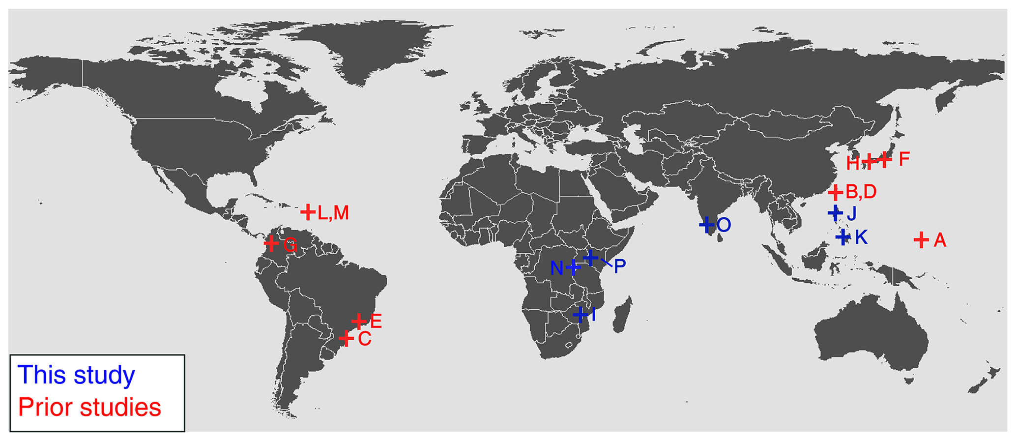
Figure 1 Locations of landslide inventories considered in this study. Locations labeled in red have been published previously, while those in blue are presented for the first time here. Satellite images of the newly mapped landslide inventories can be found in the Supplement. Table 1 contains the details of each of the inventories, organized in alphabetical order.

Table 1 Details of landslide inventories analyzed in this study.

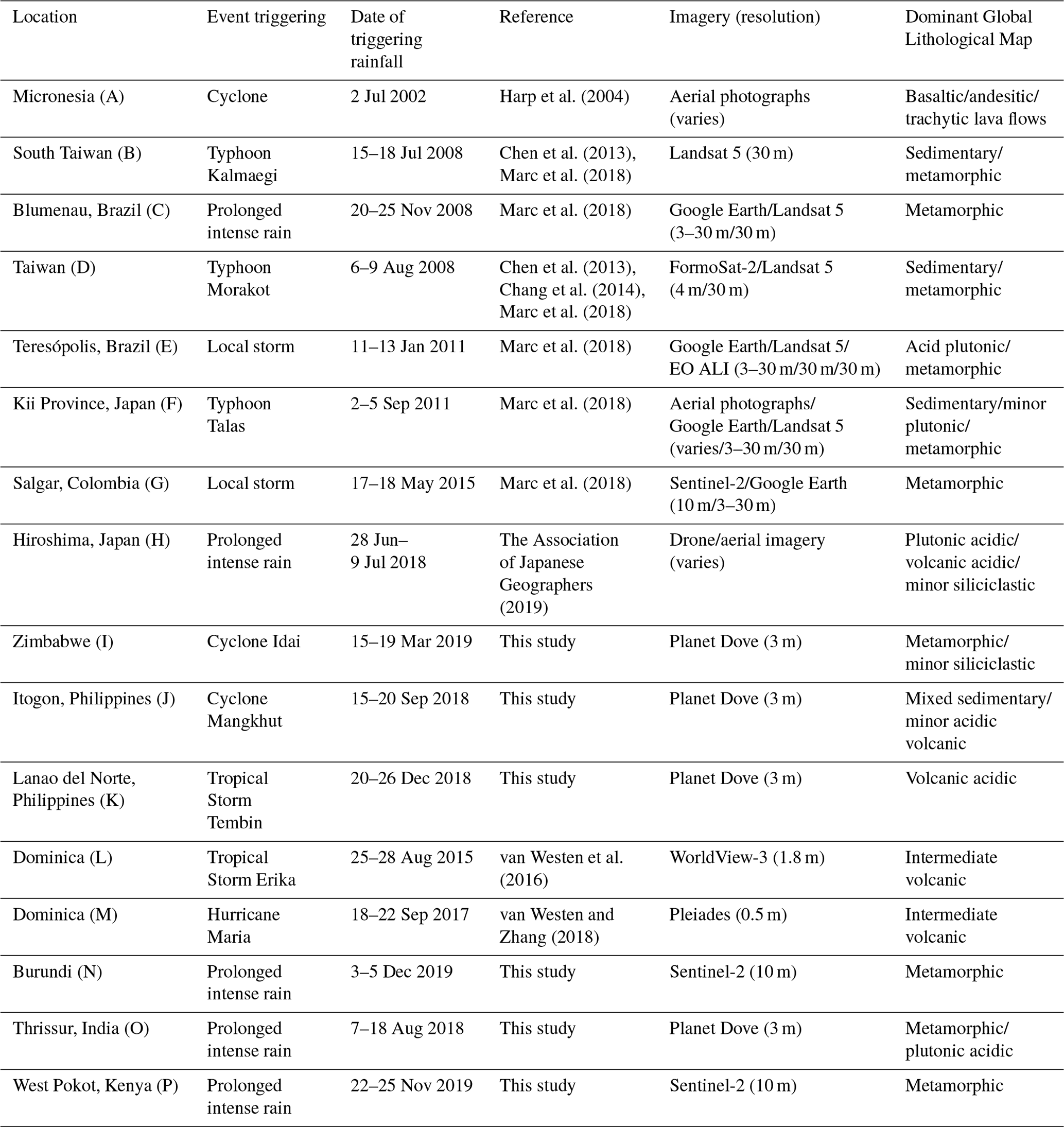
As such, we incorporate 10 existing inventories and supplement them with 6 further inventories that we have produced for this study. The details of each of the inventories are described in Table 1. For several of the newly produced inventories, we have utilized high-resolution imagery from Planet Dove satellites (Planet Team, 2017) available through the Commercial Smallsat Data Acquisition (CSDA) Program (https://earthdata.nasa.gov/esds/csdap, last access: 12 January 2022). Planet imagery represents an important step change for landslide mapping procedures, since the high spatial resolution of approximately 3 m of the images is combined with a rapid return time of the satellites (of the order of 1 image per day). For several of the newly generated inventories, we have mapped the landslides manually using GIS software. This has resulted in three inventories; two in the Philippines and one in Thrissur, India (Table 1). The remaining new inventories were generated using the semi-automatic object-based methods of Amatya et al. (2019, 2021). The algorithmic method was used to reduce the overall time spent mapping some of the larger new inventories. Since algorithmic methods are known to produce artifacts when broadly applied (Pawluszek et al., 2018) and can lead to amalgamation of individual landslides into larger polygons (Marc and Hovius, 2015), each of the automatically generated inventories was additionally corrected by manual comparison with pre- and post-event high-resolution imagery in GIS software.

Beyond the five essential mapping criteria, additional criteria include the differentiation of scar and deposit areas and the classifications of landslides according to their type/mechanisms. However, these criteria are difficult to fulfill for large event inventories (see in Tanyaş et al., 2017), especially when based on various sources of optical imagery, limiting our ability to differentiate between scar and deposit areas (Casagli et al., 2017).

The mapped inventories combine scars and deposits in the polygon delineation, although in the analysis discussed below we have sought to differentiate these areas. In terms of landslide type we could not systematically classify each landslide polygon. However, we have removed debris flows from the analysis where possible by removing long-runout landslide polygons from each mapped inventory. In general, this mapping identifies rockslides, rock avalanches, shallow soil toppling and slumping failures but does not capture slow-moving landslides where surface changes may be less evident. A focus on these kinds of landslides is warranted since the volume of material mobilized during large storms from such landslides can lead to damaging debris flows and bedload transport impacts (Badoux et al., 2014). Removing debris flows from the analysis allows us to provide consistent landslide maps that can be used to estimate volumes of mobilized landslide material, for example using global scaling relationships like those defined by Larsen et al. (2010), and permits a focus solely on the topographic characteristics of landslide source regions, rather than on the characteristics of preferential runout paths.

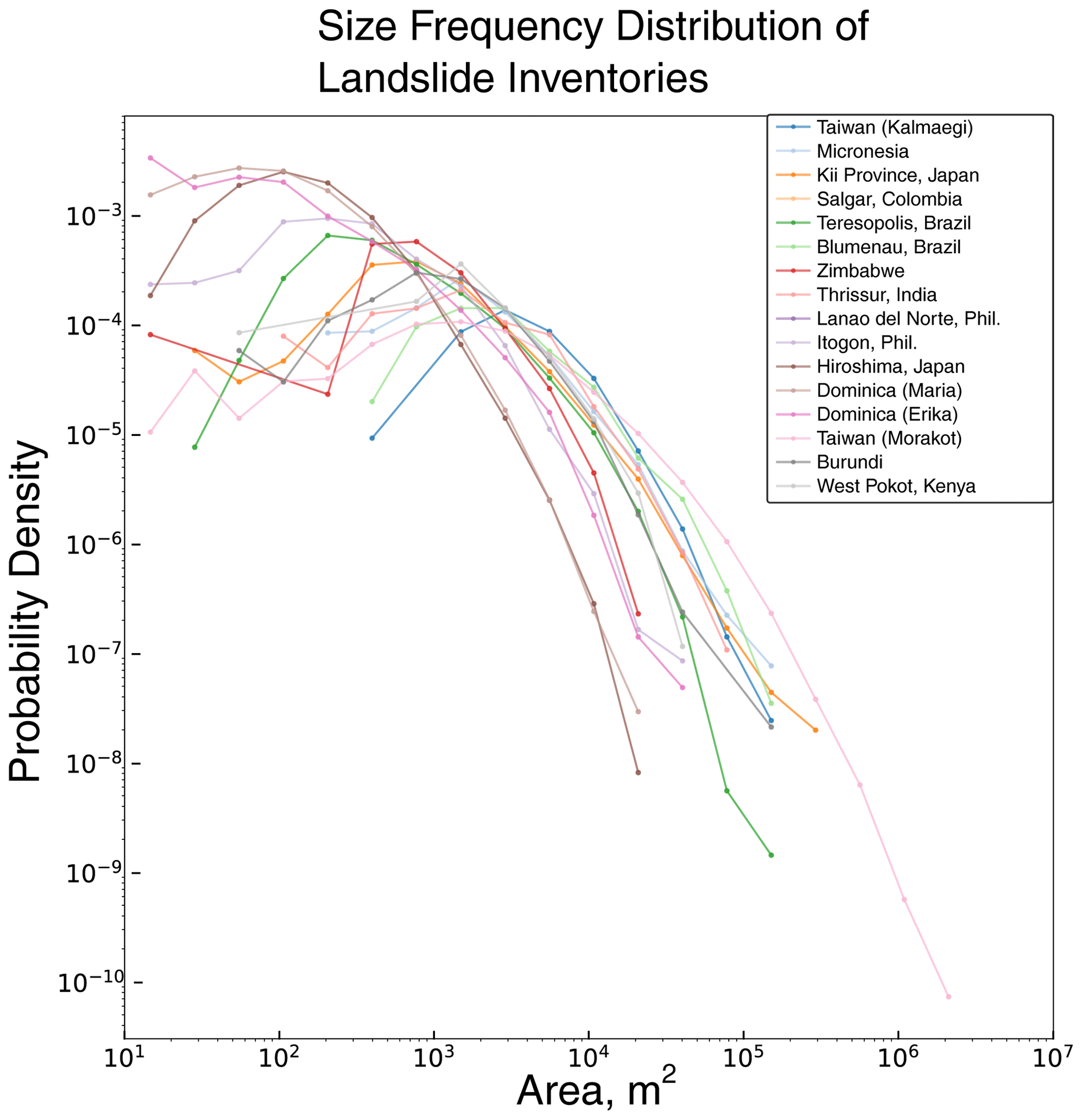
Figure 2 Probability density for landslides in each event inventory, obtained as the number of landslides with areas falling into logarithmic bins (consistent bins for all inventories), $N_{[A:A+dA]}$, normalized by the bin width, dA, and the total number of slides for the event, N_tot (see Malamud et al., 2004).

Table 2 Macro-level characteristics for events discussed, including rainfall statistics. Note that median slope values have been calculated by excluding very low slope values (<1^∘) to remove lakes and oceans.

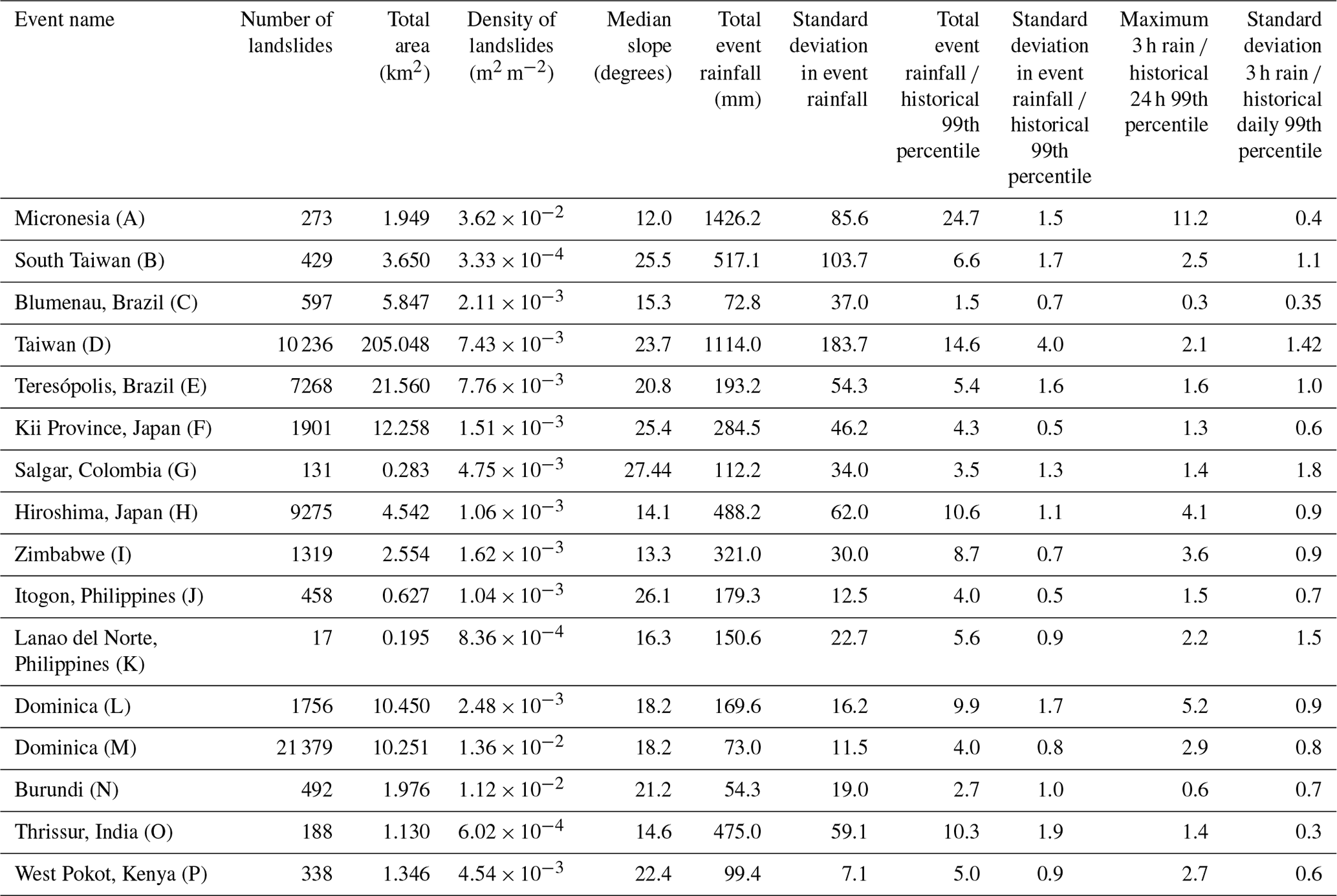
We contrast each of the inventories mapped here by comparing the size–frequency distributions of each dataset, shown in Fig. 2. For each of the inventories, we show the probability of a landslide within a given area interval, as a way to assess the frequency of small and large landslides across the different datasets. Each of these landslide events was triggered by extreme rainfall, and although it is not our intention to examine the triggering rainfall in detail in this study, it is useful to briefly discuss the characteristics of the rainfall events in question. It is important to note that the date of the triggering rainfall is not identical to the dates on which the imagery used to map the landslides was obtained. Although we have selected events where the triggering rainfall significantly exceeds historical peak rainfall (and therefore is likely to be the dominant trigger for landslides), some events may have occurred as a result of lesser rainfall before or after. While the new inventories generated for this study utilize Planet imagery that closely brackets the rainfall events (within 1 week either side), the older inventories may be more subject to this challenge. A detailed analysis of the triggering rainfall associated with several of these inventories is described by Marc et al. (2018), who used local gauge data to characterize the rainfall intensities. We were unable to find consistent local gauge data for several of the more recent events that are published here for the first time (events in Zimbabwe, Burundi and Kenya and the two events in the Philippines). We can still use satellite rainfall data as a consistent source of rainfall for each of the events, however. To assess these, we utilize the reprocessed IMERG (Integrated Multi-satellitE Retrievals for GPM) version 6B rainfall product (Huffman et al., 2020), which merges and homogenizes data from NASA's Global Precipitation Measurement (GPM) mission with its predecessor Tropical Rainfall Measuring Mission (TRMM). All of the events considered occurred within the period during which GPM IMERG v06B rainfall data are available (2001–present). Because the satellite rainfall data spatial resolution is relatively coarse, it is not possible to effectively draw comparisons between the landslide polygons and the surrounding data in the same manner as the topographic data. However, we can still characterize the rainfall occurring during each event. We have analyzed the total rainfall occurring during each of the events by accumulating the rainfall data over the period of each event indicated in Table 1 and compared this with the calculated historical 99th percentile of daily rainfall as a way to normalize each event to the historical trends. The 99th percentile is calculated empirically based on the GPM IMERG v06B record (2001–2020). Since the length of rainfall period associated with each inventory varies, normalizing by the 99th percentile for a single day provides a consistent normalizing factor for each inventory. Additionally, in Table 2 we show the maximum 3 h rainfall intensity for each of the events, normalized by the historical 99th percentile of daily rainfall. The normalized total event rainfall and normalized 3 h rainfall provide a side-by-side comparison of the overall rainfall accumulation and the maximum intensity. The values for both total event rainfall and maximum 3 h rainfall are calculated as the average across all IMERG grid cells in the area of the inventory. Table 2 summarizes information on the landslide inventory characteristics including the total landslide area, the density of landslides in the mapped area, satellite rainfall and average slope in the mapped area. Despite other studies suggesting links between event total rainfall and the density of landsliding (Chen et al., 2013; Marc et al., 2018), we do not observe clear links between the measured rainfall data and the macro-scale statistics of each landslide inventory. Relations between landslide density and rainfall can be obscured by variations in climatic and/or hydromechanical properties with each study area (Marc et al., 2019). We suggest that exploring the links between rainfall intensity as characterized by satellite measurements and the density of landsliding that results is an important topic for future research.

2.3 Topographic analysis

We have analyzed the topographic characteristics of landslide locations for the event inventories, using global satellite datasets to ensure consistency across each site. These datasets are also openly available, which supports replication of these methods and findings by other authors. In Table 3, we show the datasets we have used.

Table 3 Analysis datasets. Explanation of each of the variables is found in the accompanying text.

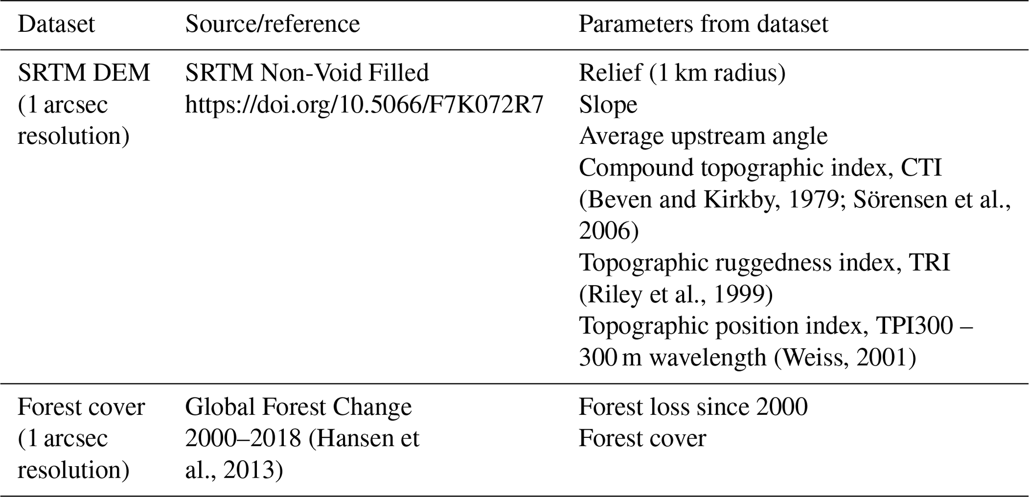
The DEM and forest loss data are both provided at approximately a 1 arcsec resolution, which means we do not have to resample either dataset when conducting a raster-based analysis at this scale. While this resolution is not as fine as some of the imagery used to map the landslides, which can be 3 m or finer, it represents the finest resolution at which these two datasets can be analyzed using non-commercial, open datasets at a global extent. We utilize forest loss data derived from Landsat imagery spanning the years 2000–2018. Cells where forest loss is observed in any year from 2000 until the year in which the landslide event occurred are considered a binary “true” value for forest loss. This does not consider regrowth of vegetation in places where forest loss was observed many years prior to the event, and as such it is a relatively blunt tool to assess the importance of vegetation to landslide location.

Not all of the topographic parameters are universally used in landslide analysis. Slope is almost universally considered for landslide modeling, but the use of others (in particular the topographic position index) is less common (Reichenbach et al., 2018). The topographic position index (TPI) (Weiss, 2001) is a quantification of the relative position of a cell within the landscape. It is calculated as the difference in elevation of each cell in a DEM from the mean elevation of a specified neighborhood around that cell, with the radius of the neighborhood chosen beforehand (in this case, 300 m). Negative values indicate the cell is in a topographic hollow, and positive values suggest that it is elevated above its surroundings. The distance over which the neighborhood comparison is made (TPI wavelength) determines the scale of the features resolved; negative values at long wavelengths indicate a position in a wider valley, while at short wavelengths this would indicate steep narrow gorges. In this study, we focus on short-wavelength TPI values since this aligns more closely with the scale of the landslide features. Relief indicates the difference between minimum and maximum elevation in a given window. It is a proxy for both slope and the size of hillslopes; higher-relief zones have been shown to be associated with landslides in many locations (Reichenbach et al., 2018). The compound topographic index (CTI) is a measure of both slope and the upstream contributing area. It is calculated by the formula $\ln (a/\tan b)$, where a is the flow accumulation area per pixel and b is the local slope in radians. In some locations the CTI is correlated with soil parameters such as thickness (Liang and Chan, 2017). We also calculate the topographic ruggedness index (TRI), a measure of the local surface roughness. It is defined as the root-mean-squared difference in elevation between a central pixel and each of its 8 neighboring pixels.

Finally, we also analyze the average upstream angle – this is the average angle from the pixel location to every cell that drains into that pixel. It provides a measure of how steep the areas are that feed into each pixel. There is a significant degree of overlap between how some of these parameters are calculated, and we recognize the importance of considering co-linearity.

In order to assess the co-linearity of the variables, we have compared each pair of variables. Pair plots are shown in the supplementary material (Figs. S1 and S2 in the Supplement). Unsurprisingly, strong correlations are observed between slope and the average upstream angle, as well as between topographic ruggedness and relief. It is also important to note the negative relationship observed between the TPI and CTI, confirming that the hollows in the landscape are also locations where the saturation state is likely to be higher. Considering these co-linear relationships, it is important to ask which variables are the most effective predictors of landslide locations for the analyzed inventories. To analyze the importance of the input variables, we first perform analysis of the influence of each individual variable as a bivariate analysis (Sect. 3.1) and then use a generalized linear model to explore the effect of co-linearity (Sect. 3.2).

For the assessment of each parameter by itself, we calculate the relative ratios of the distributions for each variable for the topography and the landslide populations. The topography values are calculated for all pixels within the area in which landslides were mapped. Since we lack data on the mapped areas for all of the inventories, we assume that the convex hull (minimum bounding polygon) for the landslide polygons represents the mapping area. This follows the example of other recent studies (Marc et al., 2018; Milledge et al., 2019). For both the landslide parameter distribution and the parameter distribution for the topography, we divide the values into bins, normalizing by the total size of the distribution. This essentially represents a value–frequency distribution. For each of the bins, we then divide the landslide probability by that of the topography to obtain a ratio. Using slope as an example, this provides an estimate of the probability of a landslide occurrence at a given slope value compared to the occurrence of that slope in the landscape. This step is meant to explore the significance of each variable in a bivariate structure (Fig. 3).

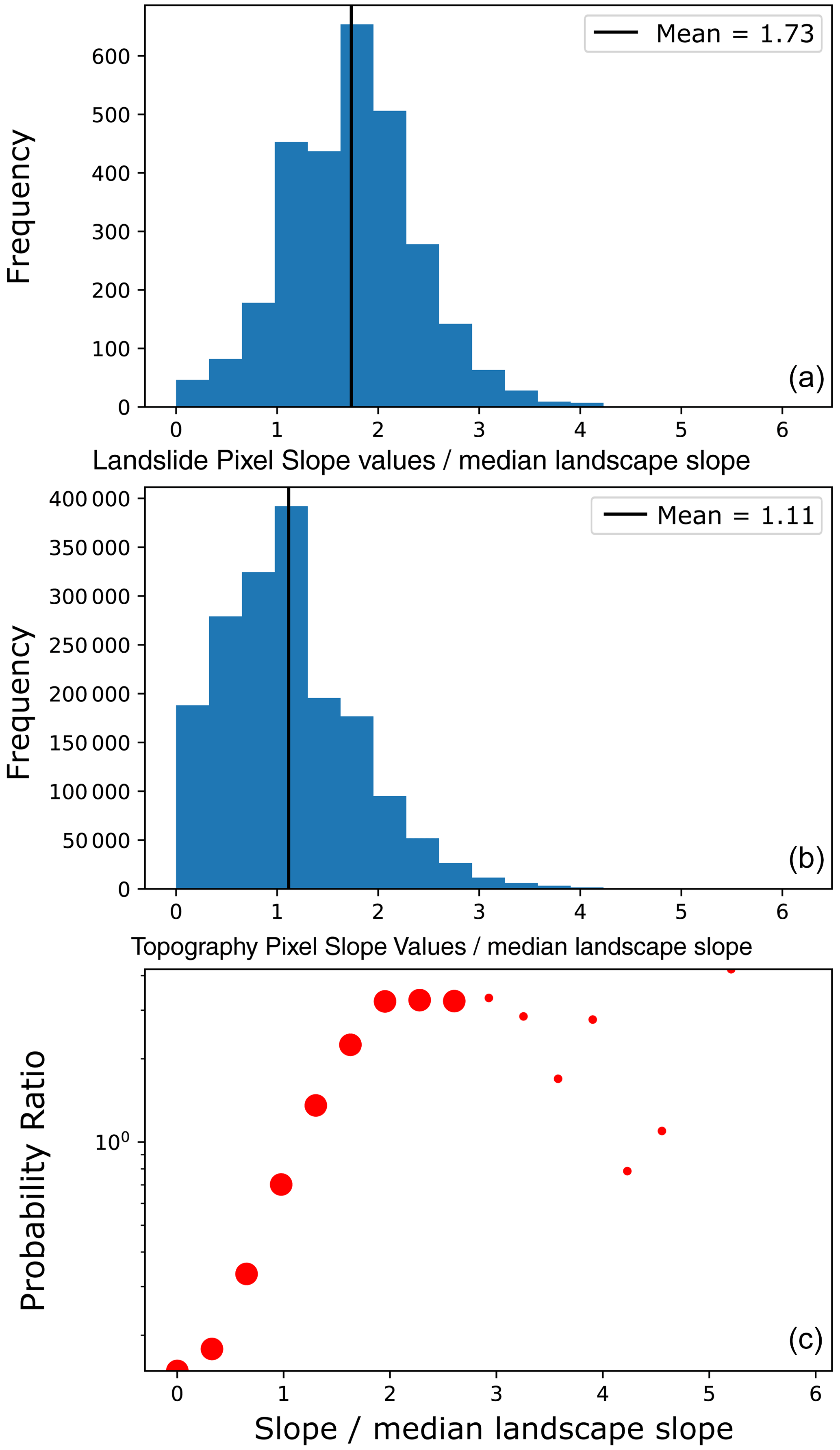
Figure 3 Example of landslide : topography ratio comparison for landslides in Zimbabwe triggered by Cyclone Idai. This shows the distribution of values for landslides (a) and topography (b) for slope. The lower part of the figure (c) shows the relative ratio of the two distributions for the parameter. The black lines in (a) and (b) illustrate the mean value of the data. In the lower figure (c), the size of the points depends on whether the difference between landslide and topography exceeds the calculated confidence interval for that bin interval; larger points indicate significant deviation (p>0.95), and small points indicate the difference is not significant at that probability level.

We characterize the landslides in two ways – first, by calculating the parameter value for the scar area of the landslide and, secondly, by calculating the raster values for the entire landslide body. We lack consistent data on the scar area for the landslide inventories in question, so instead we calculate an approximation of the scar area based on the geometry of each individual landslide. We utilize the method of Marc et al. (2018) to extract the scar areas, which uses the perimeter and area (A) of landslide polygons to calculate the aspect ratio of an equivalent ellipse, K (Marc and Hovius 2015), and the associated width (W), according to the formula $W\cong \surd (\mathrm{4}A/\mathit{\pi }K$) (Marc et al., 2018). The scar area is defined as ∼1.5 W² based on a global database of the scar aspect ratio (Domej et al., 2017). For each scar, we calculate the average value within the polygon area of each parameter. This avoids bias toward landslides with long runouts and effectively removes the lowest portion of the polygons which may not have the same topographic signal as the source areas. Even if the scar areas are only approximate, focusing on the upper part of the landslides is warranted for an improved understanding of the topographic control on landslide susceptibility.

The second way of characterizing the landslide – assessing the overall area of the landslide – allows us to focus on areas in the landscape that are likely to be hazardous, including areas where landslide material may end up.

To calculate the parameter distribution for the whole landslide body, we first rasterize the polygons of landslide locations to the resolution of the SRTM DEM (1 arcsec). This provides a binary raster of landslide presence. We then assess the parameter values for each of the pixels where landslides are present. This does mean that the largest landslides are most strongly represented in the distribution, but this is intentional as it permits us to focus on all of the areas affected in the landscape. It is important to note this approach – counting all pixels – is not appropriate for statistical susceptibility analysis, since it could lead to highly dependent datasets. For hazard analysis purposes, we feel it is appropriate to consider all pixels, since larger landslides are consistently more damaging, and we seek to capture the entire footprint.

In Fig. 3, an example of the comparison is shown for the landslides occurring in Zimbabwe as a result of Cyclone Idai. We show upstream slope as an illustrative parameter. To compare the landslide data with the topography, we split the data into bins, using the same bins for both landslide and topography. The probabilities of the landslide and topography values are then compared with one another. To allow for more consistent comparison of inventories with diverse topography, we normalize the landslide and topography data by the median value for the parameter in question prior to splitting the data into bins (Marc et al., 2018; Milledge et al., 2019). This specifically results in the normalized conditional probability (Milledge et al., 2019). For example, in the case of slope, we calculate the median slope value for all pixels within the mapped area for each inventory and divide each binned interval by the median slope value calculated across the mapped area. Finally, for each bin, we calculate the confidence interval for the comparison of topography to landslides using the method of Rault et al. (2019).

We have generated these estimates for each of the variables listed in Table 3 and for each of the landslide inventories listed in Table 1. One of the variables – forest loss – is a binary variable – it is calculated as forest is either lost or not. As such, we can only compare the average value for landslides and for topography at large to obtain a relative difference in the average forest loss value.

Because landslides are triggered as a result of a complex interaction between various factors, we also analyze the inventories using a multivariate regression scheme to consider the interactions between the topographic factors. We do so by fitting a binomial generalized linear model (GLM) for each landslide inventory. We also apply a feature selection algorithm to identify the significant and irrelevant variables to feed the GLM. For this purpose, we use the least absolute shrinkage and selection operation (LASSO) technique (Tibshirani, 1996). This method is particularly suggested for landslide susceptibility assessment to reduce the large number of highly correlated predictors without losing parameter interpretability (e.g., Camilo et al., 2017). GLM fitting with a LASSO implementation is carried out by using the R (R Core Team, 2018) “glmnet” library, which was made available by Friedman et al. (2021). We apply this method and couple it with the 10-fold cross-validation to remove non-informative covariates and to assess the modeling performance based on the area under the receiver operating characteristic curve (AUC) calculated for each landslide inventory (Hosmer and Lemeshow, 2000). From each model we built, we store the information related to the regression coefficients. Before fitting the regression model, we apply a mean zero and unit variance normalization to all variables (e.g., Lombardo et al., 2018), which are expressed in different ranges and on different scales. This normalization allows us to better examine the modeling results in terms of the contribution of each variable. In this scheme, larger absolute values of the regression coefficients refer to a relatively large contribution of variables.

We have combined the results from each individual inventory into a single figure for each of the variables to assess relative differences, as well as which variables are most strongly associated with where landslides are mapped.

3 Results

3.1 Bivariate analysis

The bivariate analyses show that several of the parameters are strong predictors of the location of both the scars and the overall area of landslides, and while there is significant variability between the different inventories, there are consistent patterns that emerge across all events. In broad terms, we find that rainfall-triggered landslides occur more often in rough, steep terrain (Figs. 4, 5 and 7). Results from the compound topographic index (CTI) and short-wavelength topographic position suggest that these parameters can be used to effectively distinguish between scars and the entire landslide area, with a high probability of scars at low CTI values and at more positive TPI values (i.e., landscape convexities). For all metrics, we find that all studied inventories have approximately equal sampling at the median landscape value. This can be observed in Figs. 4–8, where the probability ratio of 1 for almost all inventories occurs at approximately the median value of the parameter for the entire landscape. In other words, the transition from low to high landslide probability is relative to the local landscape median value and not to an absolute value of the considered metric.

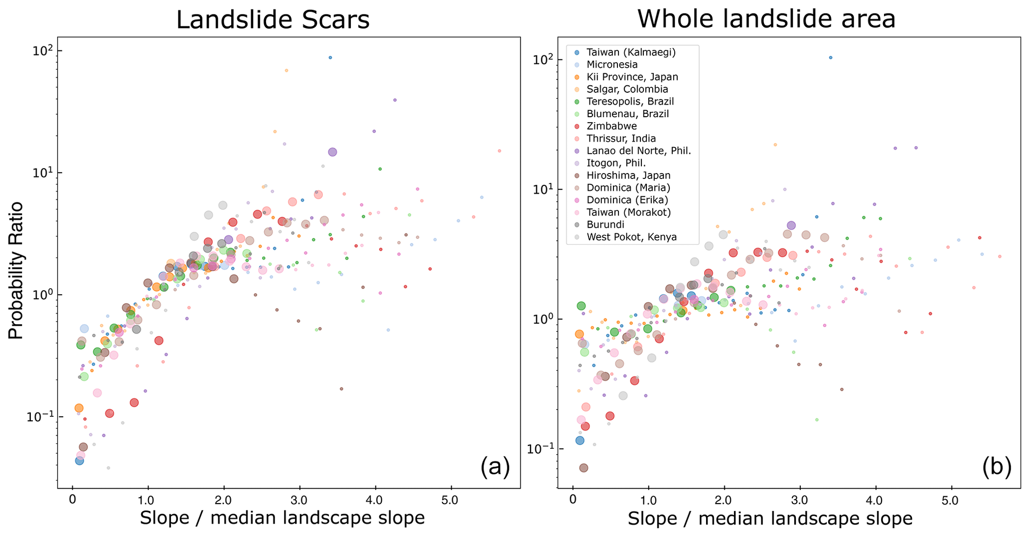
Figure 4 Landslide probability ratio against the slope normalized by the median of the local landscape, for the scar area (a) and the whole landslide area (b). The size of the points depends on whether the difference between the landslide and topography exceeds the calculated confidence interval for that bin interval; larger points indicate significant deviation (p>0.95), and small points indicate the difference is not significant at that probability level.

For all of the events, there is a general increase in landslide probability at higher slope values (Fig. 4). Similarly, a strong increase in landslide probability is observed for the average upstream slope angle (Fig. 5). The distributions of the different inventories are slightly tighter than for slope, indicating that this may be a more consistently applicable variable. Specifically, we note that both scars and whole landslides are at an equal sampling level at the median landscape upstream angle, strongly undersampling and oversampling the gentler and steeper slopes, respectively (i.e., proportionately more landsliding at higher slope values and less at lower slopes). This can be observed in Fig. 5. Consistent trends emerge where results are within a 95th-percentile confidence interval, although there is a greater spread of data values where results are not considered statistically significant.

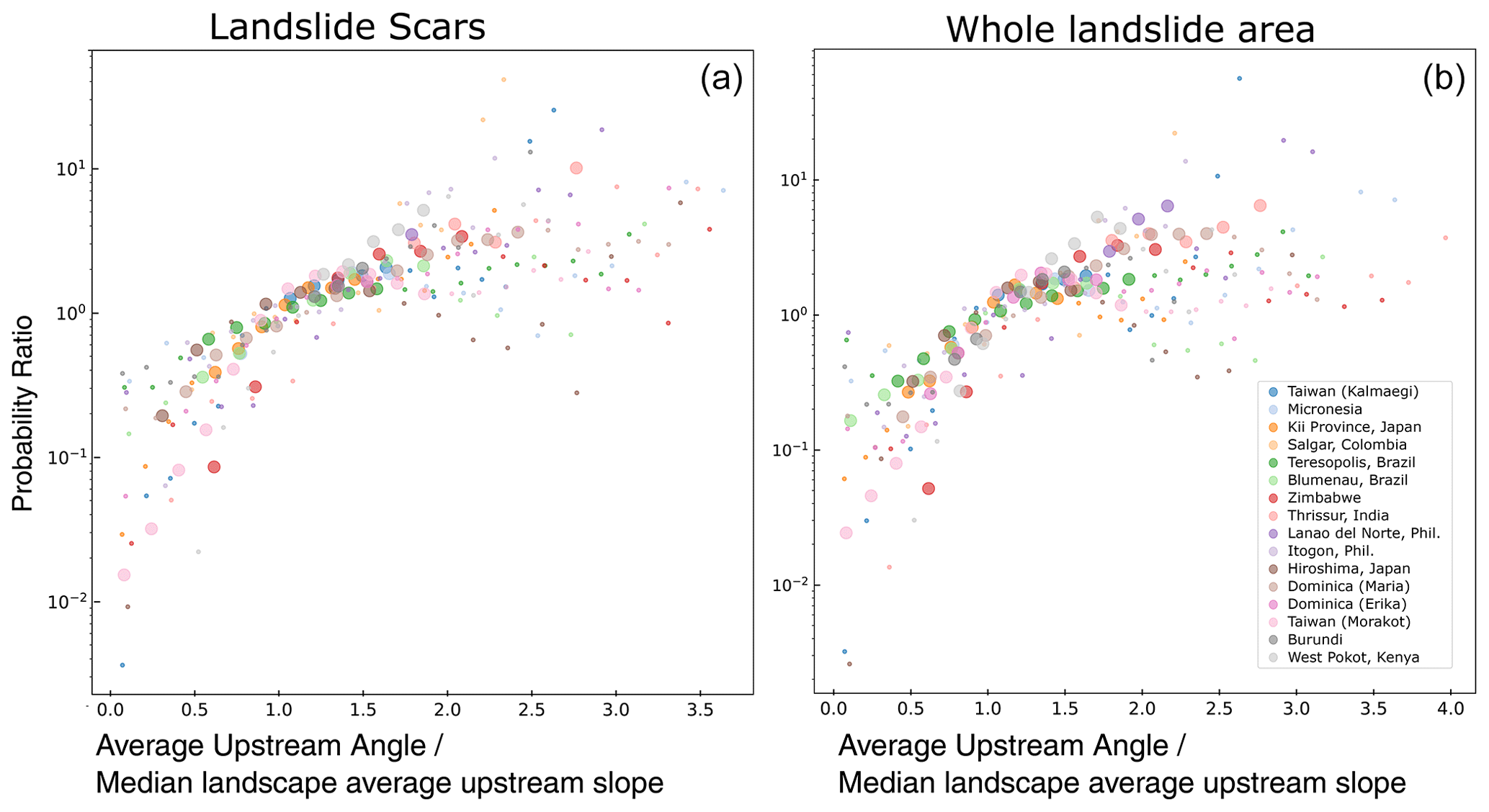
Figure 5 Landslide probability ratio against the average upstream angle normalized by the median of the local landscape, for the scar area (a) and the whole landslide area (b). The size of the points depends on whether the difference between the landslide and topography exceeds the calculated confidence interval for that bin interval; larger points indicate significant deviation (p>0.95), and small points indicate the difference is not significant at that probability level.

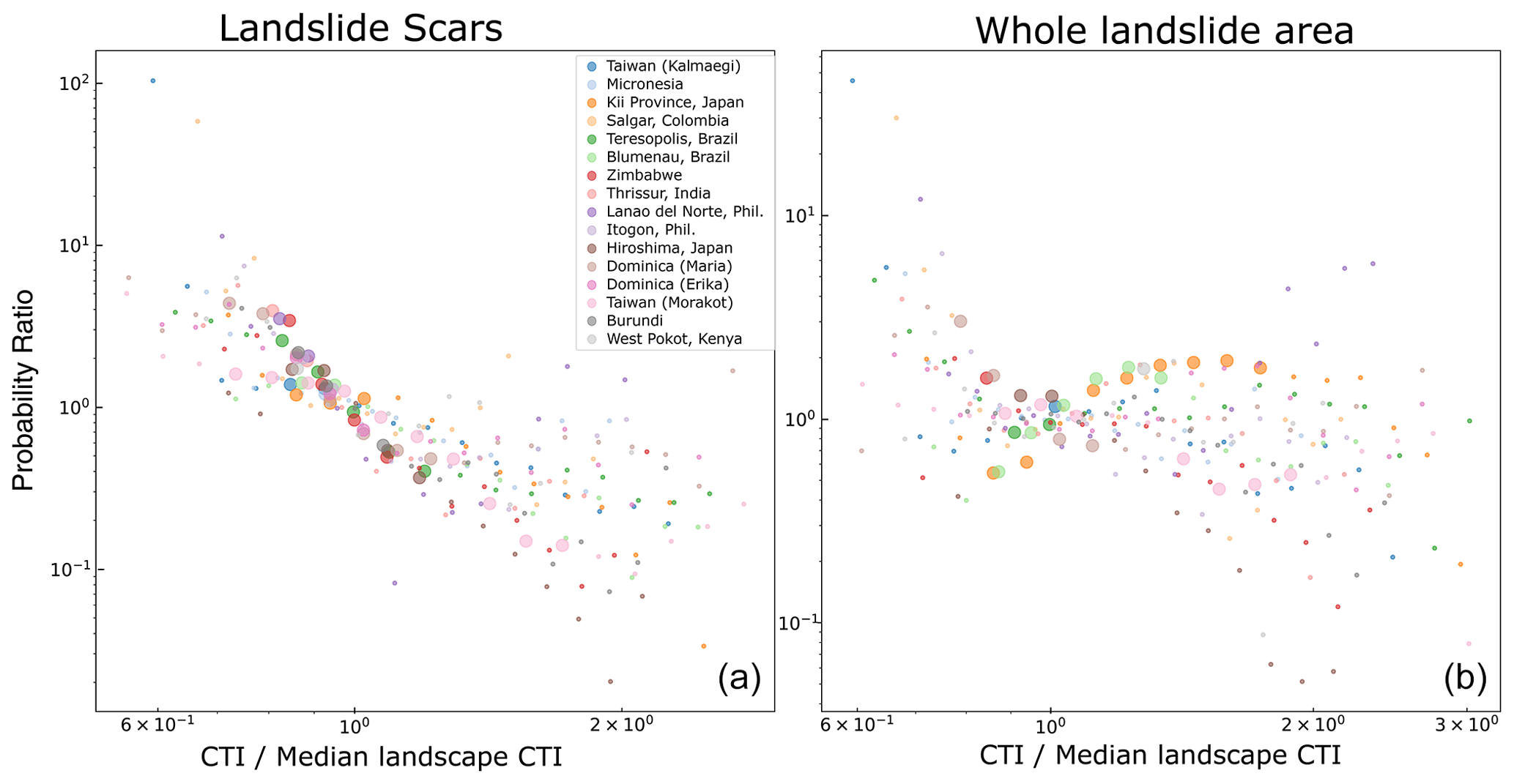
Figure 6 Same as Fig. 4 but for the compound topographic index (CTI). Note that the x axis is a logarithmic scale.

Figure 7 Same as Fig. 4 but for the topographic ruggedness index (TRI).

The compound topographic index (sometimes referred to as the wetness index), when tested for landslide scars, shows higher probability of landslides for lower CTI values (Fig. 6). This trend is negligible for whole landslide areas, with the statistically significant points showing almost no variation in landslide probability with a changing CTI. This suggests broadly that the CTI is a poor predictor of the areas where landslide hazard may be increased but a better predictor of the source locations. The relationship between scar probability and the CTI is not strongly linked with flow accumulation, despite the role that flow accumulation plays in setting the CTI. In Fig. S3 we show the probability ratios for flow accumulation values, and no clear relationship emerges between the probability ratio and flow accumulation. This suggests that the slope component of the CTI is more important when considering scar locations, while the flow accumulation factor (observed to be correlated with an increase in probability of whole landslide areas) may be offset by the slope in the areas where landslides run out, leading to no overall correlation with the CTI and whole landslide area.

Additionally, we observe that the CTI value where landslide scars and topography are equally sampled is approximately the median value, and the fit for each inventory is relatively consistent.

Figure 8 Same as Fig. 4 but for relief in a 1 km radius of each cell.

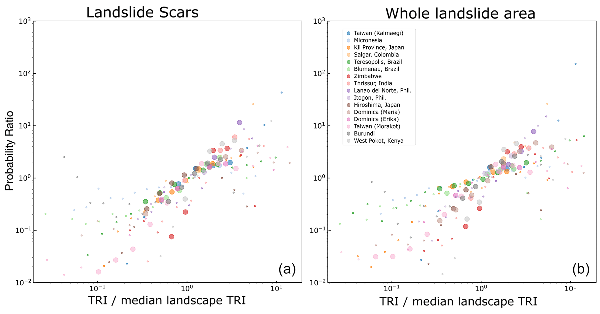
We find that the topographic ruggedness index is also a relatively strong predictor for landslide probability, with increases in the TRI correlated with increases in the landslide probability ratio for almost all events (Fig. 7), and statistically significant results are observed for several of the inventories. For several events, the results are in line with prior work that has shown roughness and related metrics to be correlated with landslide occurrence (Costanzo et al., 2012; Reichenbach et al., 2018). While the point of equal sampling of landslides and topography is approximately the median value for the inventories analyzed, the slope of the relationship diverges somewhat above and below this point. This suggests that the most heterogeneous parts of the landscape may not be as strong a predictor for landslide occurrence as areas of high slope.

There are not strong systematically consistent relationships between relief at a 1 km scale and the probability of landslide scars and total areas. Some increase in probability is observed with increasing relief, although this is saturated at relief values above the median relief. This suggests that relief alone is a relatively poor predictor of the source areas of landslides or that the resolution of relief may be too coarse. In a few cases – Burundi, Typhoon Morakot in Taiwan and Kii Province in Japan – there is a slightly clearer increasing relationship.

We observe a link between the short-wavelength topographic position index (300 m assessment radius) and landslide probability ratios for landslide scars in several, but not all (i.e., not Kalmaegi, Morakot and Kii), of the events (Fig. 9). Specifically, landslide scars are significantly more likely at positive TPI values (short-wavelength landscape convexities like ridges). Although this is the case for the majority of inventories, results from both inventories in Taiwan and Dominica do not exhibit this tendency. This parameter also shows the clearest distinction between the scar areas and the whole landslide areas. The entire landslide area is more likely to be found at negative TPI values (landscape concavities like valley bottoms). While the TPI at the 300 m wavelength does not demonstrate quite as consistent relationships as slope or the CTI, it remains a strong predictor. In particular, the larger variation between scars and overall landslide areas suggests that short wavelengths may be a valuable way to distinguish between scarps and deposits in a preliminary assessment.

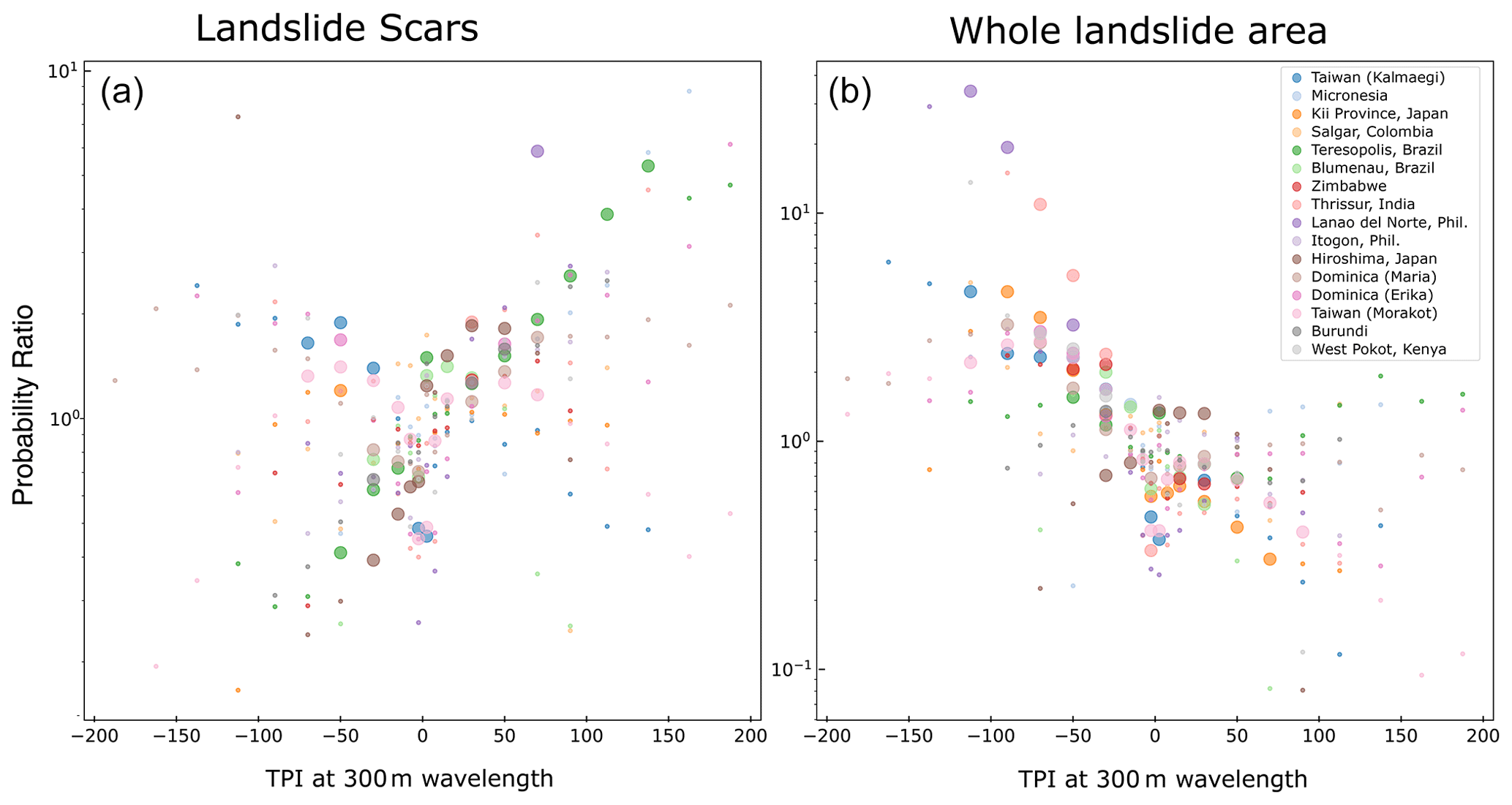
Figure 9 Same as Fig. 4 but for the topographic position index (however, here we omit normalization given that the TPI is a zero-centered variable) with an analysis window radius of 300 m.

Since forest loss is a binary variable, we do not plot this across multiple bins. However, we calculate the average ratio of forest loss in landslide zones to the overall topography, and we find across all events that the value is 1.98±1.38 (1 SD – standard deviation). This implies that forest loss zones are correlated with higher probability of landsliding. We see the largest differences between landslide zones and non-landslide zones in Salgar, Colombia, and Hiroshima, Japan, and the landslides triggered by Typhoon Morakot in Taiwan (forest loss is more than 3.5 times more likely in landslides in these cases). In four cases, forest loss was observed as less likely in landslide pixels: in Blumenau, Brazil; Lanao del Norte, the Philippines; Thrissur, India; and West Pokot, Kenya. We suggest that while forest loss prior to landslide events is generally higher in landslide locations than in the rest of the landscape, this relationship is not consistent enough to necessarily be a good predictor of landslide location by itself.

3.2 Multivariate analysis

We have used the LASSO method to quantify the importance of the different predictors for both scars and whole landslides while reducing the influence of co-linearity (Camilo et al., 2017) (Fig. 10).

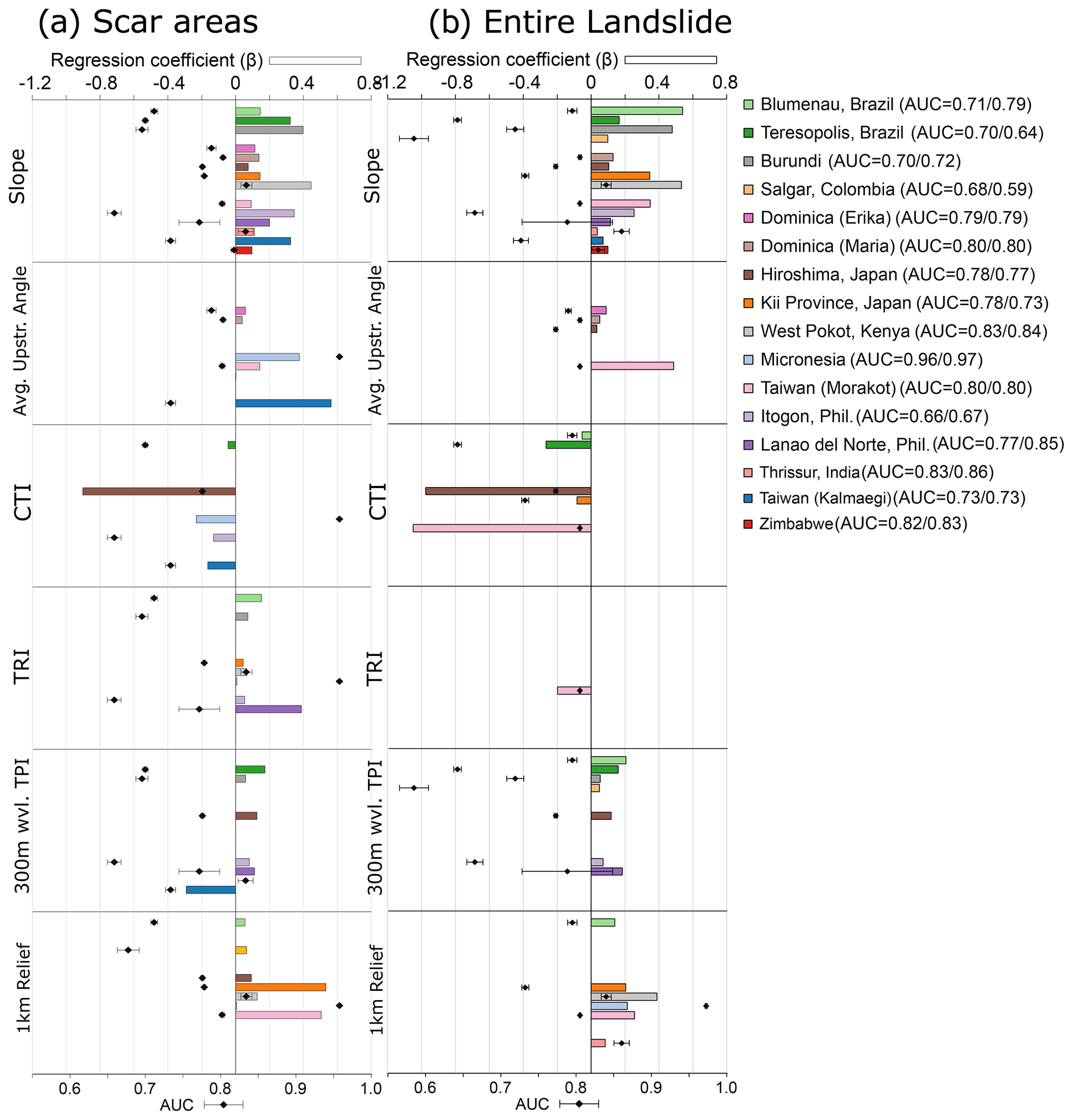
Figure 10 Figure showing regression coefficients and corresponding AUC values calculated from the fitted GLM for each landslide inventory, considering scars (a) or the whole landslide area (b). The error bar corresponds to the variation in the AUC distribution across 10-fold cross-validation replicates. Regression coefficients are not shown for predictors considered not significant by the LASSO methods. The AUC values shown in the legend are for scars (prior to slash) and entire landslides (second value).

Figure 10a and b also show the modeling performances, which are represented by AUC values, varying from “reasonable” ($\mathrm{0.6}<\mathrm{AUC}<\mathrm{0.7}$) to “adequate” ($\mathrm{0.7}<\mathrm{AUC}<\mathrm{0.8}$) and “outstanding” ($\mathrm{0.8}<\mathrm{AUC}<\mathrm{0.9}$) based on AUC classes defined by Hosmer and Lemeshow (2000). The lower AUC values for some events may indicate that we lack some key explanatory variables; crucially, this may include rainfall intensity and duration, although as discussed above we lack consistent high-resolution data to assess this within the spatial domain of the considered inventories. Other relevant parameters may include land cover, lithology and geo-structural parameters, and anthropogenic influence (Reichenbach et al., 2018).

Our findings show that slope, on one hand, is the factor that most frequently appears as significant in the GLM run for both the landslide scars and the whole areas, with landslides favoring steeper locations. On the other hand, the average upstream angle and CTI in the GLM of the scars and the average upstream angle, CTI and topographic position index (with a 300 m radius) in the GLM run for the whole area appear as the least commonly observed significant variables. The non-significant or low impact of most of these topographic variables is likely due to the co-linearity existing between these variables (e.g., slope and average upstream slope, slope and CTI, CTI and TPI – Figs. S1 and S2).

The results indicate that except for the CTI, all variables have a positive weight on classifying a given grid cell as “landslide presence” instead of “landslide absence” given the choice of predictors. There are only two cases that do not follow this general trend (i.e., the two Taiwanese inventories).

The regression coefficient of the TPI calculated for the landslide scar areas for Typhoon Kalmaegi, Taiwan, has a negative sign, unlike all other cases. Overall, as we explained above, different TPI values refer to different subsections of a hillslope. Specifically, positive values refer to ridges or hillslopes, whereas negative values correspond to the valley. As a result, the negative weight of the TPI on classifying the landslide presence and absence condition in the GLM is difficult to interpret. This could be caused by interactions between variables. Although we run a variable selection method (i.e., LASSO), the TPI could be still interacting with the others. If it shares a similar signal to at least one other variable, the sign of the regression coefficient can be influenced by the interaction.

The negative regression coefficient of the TRI obtained for the whole landslide areas for Typhoon Morakot, Taiwan, is the other case where the response of the covariate is different from the other examples. Similarly to the Kalmaegi inventory case we presented above, the negative sign could also be caused by the interactions between variables. However, this could also be associated with the physical properties characterizing whole landslide areas. The TRI in the case of Typhoon Morakot, Taiwan, in particular, might correspond to smooth topography. In either case, the TRI does not appear as a significant variable other than in case of Typhoon Morakot, Taiwan.

The two inventories where negative CTI values are most significantly associated with landslide incidence – Morakot and Hiroshima – have few commonalities; their lithologies differ, and the mean slope of the affected area in Hiroshima is markedly lower than for Morakot. Perhaps the most significant commonality is that the triggering rainfall exceeded the historical maxima by a significant degree (Table 3), which may increase the likelihood of failure resulting from local transient pore pressure increases, rather than due to saturated flow at the base of hillslopes. Excepting these two examples, the results show that the signal of the CTI does not contribute to the GLM while classifying landslide presence or absence.

4 Discussion

The primary intention of this study is to assess the critical topographic parameters associated with rainfall-triggered landslides, using a large dataset of landslide inventories that includes six newly mapped events. Our results are comparable with existing studies (e.g., Marc et al., 2018; Milledge et al., 2019) exploring landslide locations using inventories while adding more detail and assessment of global variability, which we discuss below. First, however, we explore some of the limitations and assumptions that go into the mapping and analysis of the landslides.

4.1 Uncertainty in landslide mapping and DEM metrics' extraction

Firstly, it is important to consider how representative the landslide inventories are. We have attempted to include landslide maps from a diverse set of locations around the world, but this is still only a fraction of landslides that have occurred in the last 2 decades. Some of the inventories, like the landslides occurring due to Typhoon Morakot in Taiwan, are driven by such huge rainfall events that the overall area of landsliding greatly exceeds other examples with lower rainfall. This is one of the key reasons why we have used probability ratios as a metric to assess landslide locations, since they do not consider the overall area of landslides triggered by a given rainfall event. Most of the inventories are drawn from locations with tropical climates (Geiger, 1954), and although the pairs from Brazil and Japan sample areas of humid subtropical climates, this is not a true representative sampling of climatic regimes. One exception is the landslide inventory from Zimbabwe, which is in a semi-arid climatic region. Although our examples disproportionately sample tropical and subtropical areas, these areas generally experience the highest erosion rates (Milliman and Syvitski, 1991), driven by increasingly intense rainfall (e.g., Bookhagen and Strecker, 2012). Similarly, while the inventories are drawn from places with diverse lithologies, we do not have datasets from a fully representative set of lithological locations (Hartmann and Moosdorf, 2012; Table 1).

Although we have used hand corrections to reduce the impact of polygon amalgamation from algorithmic mapping methods, some inconsistencies may still exist. One important consideration is that the datasets used here do not distinguish between different landslide types or distinguish between scar and deposit. While this is consistent across inventories, it is important when considering the results. In particular, since we do not have constraints on whether mapped landslides are purely shallow soil slides or whether they incorporate deeper bedrock, we cannot determine differences in topographic characteristics associated with each. The change in material properties from soil to bedrock can lead to changes in overall volume mobilized for a given landslide area (Larsen et al., 2010), so inventories where smaller shallow landslides are a larger proportion of the mapped inventory may have different characteristics. For example, the landslides mapped using aerial photography around Hiroshima, Japan, do not show particularly high probability ratios at very high relief or TRI values, suggesting these landslides generally occur on smaller less rough hillslopes.

Hand mapping and correcting will help reduce the potential for landslide amalgamation (Marc and Hovius, 2015), which is essential in order to estimate width and scar areas from landslide polygon geometry (Marc et al., 2018). Since we do not have access to the imagery for all of the previously published events, we are not able to correct these events and thus must rely on prior mapping being consistent with our own efforts. Part of the challenge of compiling different events is the different sources of imagery used to create each inventory. For most of the inventories we have mapped as part of this study, the imagery is consistent in terms of resolution, and we have benefited from the rapid return time of Planet Dove satellites to ensure that cloud cover does not mask any of the areas mapped. However, without imagery to clarify, it may be possible that parts of the previously published inventories are masked by cloud cover. In addition, the inventories mapped using coarser-resolution satellite imagery, such as the part of Taiwan impacted by Typhoon Kalmaegi, may not capture the smallest landslides that resulted. If smaller landslides are preferentially found in certain parts of the landscape, this may introduce systematic biases in observed probability ratios.

While the imagery used to compile the different inventories varies in resolution, there do not seem to be consistent, systematic differences between probability ratios that can be explained as a result of small landslides that systematically bias the events. For example, landslides in the Dominica events have similar probability ratios for each parameter compared to the landslides from Typhoon Kalmaegi in Taiwan, despite these datasets having the largest difference in effective imagery resolution.

When considering the whole landslide area, we pixelate the landslides to the resolution of the DEM to highlight the most hazardous parts of the landscape. This pixelation process can introduce a source of systematic error, since if less than half of a cell area is occupied by a landslide polygon, it is still considered to be a “landslide pixel”. Some landslides may be significantly smaller than the SRTM cell resolution if they are mapped using high-resolution imagery, but they will still count as a full-size pixel for the purposes of analysis as a result of the rasterization process. This introduces a potential source of bias as smaller landslides may make up a larger proportion of analyzed pixels than their actual area would represent. Landslides below the approximate area of half an SRTM cell (450 m³) make up an appreciable proportion of the total landslide area in Hiroshima and Dominica (∼30 %) (Fig. S12). In these settings, we would expect that the influence of smaller landslides may be over-estimated at the 30 m resolution of analysis, although in the majority of other inventories landslides below this cutoff represent less than 5 %–10 % of the total landslide area (and therefore the analytical dataset of landslide pixels).

To address the potential for bias due to oversampling of small landslides with a coarse-resolution DEM, we have resampled the DEM for the events in Hiroshima and Dominica to a resolution of 10 m, at which nearly all landslides are captured without size exaggeration. We then recalculate the probability ratios for the landslides and compare the resampled DEM results with those from the original DEM (Fig. S5). For the slope, average upstream angle, CTI, relief and TRI, only minor differences are observed between the results for a resampled DEM and the original DEM. There are some differences between the TPI at a 300 m resolution, but no consistent relationship seems to emerge. Thus we do not think our results are affected by the coarse rasterization process, although it is likely that accessing a higher-resolution DEM may alter the result depending on the local variable, like the slope, CTI or TRI.

Other parameters are often incorporated into landslide susceptibility such as geological factors like soil characteristics or lithology, local land cover type, or climatic metrics. Although global data for rainfall, soil type and geological parameters exist, the resolution of these datasets is too low to allow for consistent comparison of landslide and non-landslide areas at the scale of the analysis described here (∼100 m). As such, we have chosen to focus exclusively on topographic factors within our assessment.

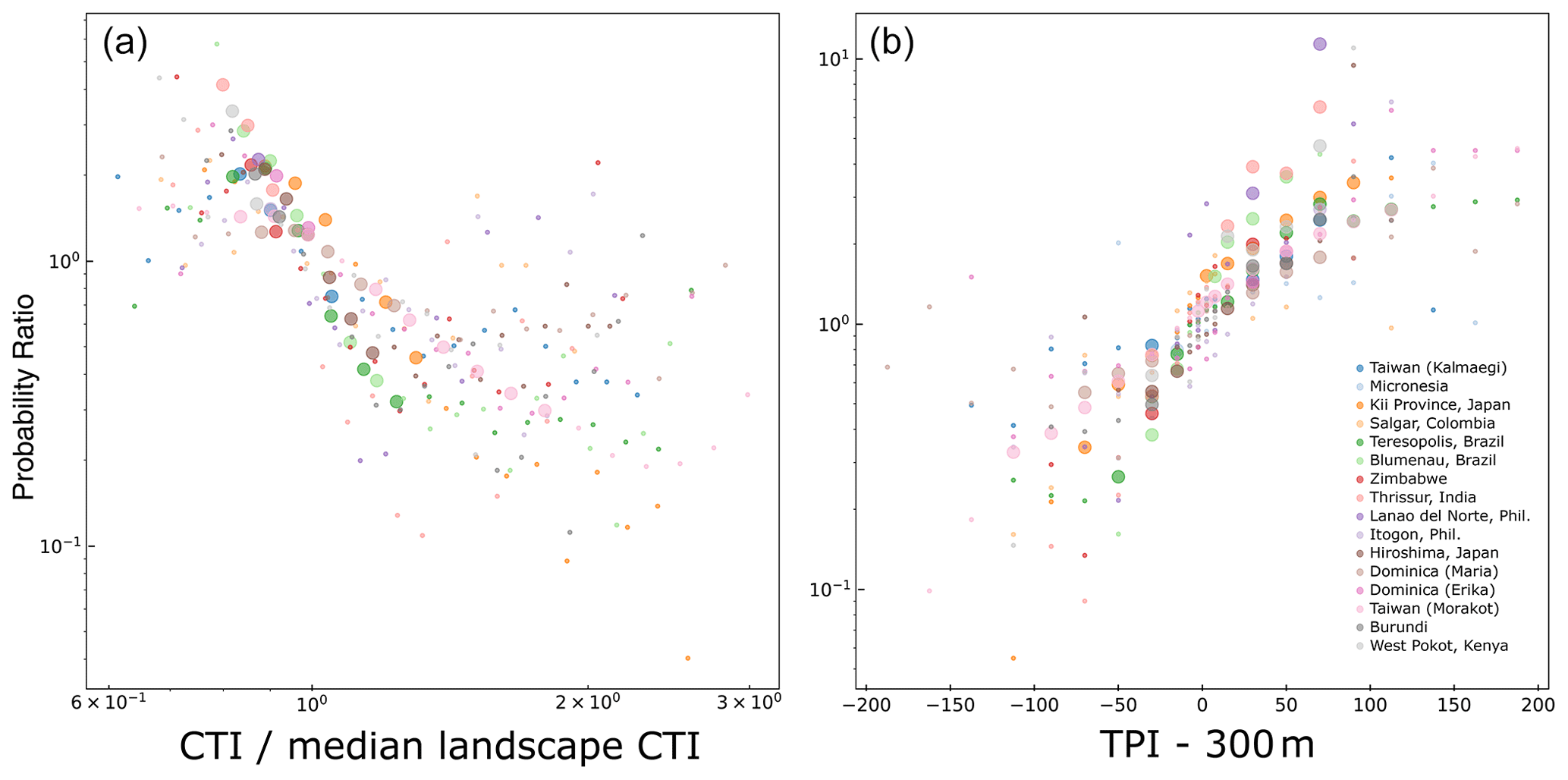
Figure 11 Probability ratio of landslide scar areas compared with the entire landslide area. It is important to note that while Figs. 3–9 contrast the landslide areas (scar or entire mapped area) with the topography, this figure shows the ratio of probabilities for the scar and whole landslide area. Specifically, this shows the probability of a scar at a given CTI value, normalized by the probability of that CTI value, divided by the probability of the entire landslide at a given CTI value, normalized by the probability of that CTI value. Higher values indicate that scars are more likely than whole landslide areas at that parameter value. Panel (a) shows the result for the CTI and panel (b) for the short-wavelength TPI.

4.2 Differences between scar and overall landslide area

While for several parameters, scars and the entire landslide area are similarly sampled at a range of values, for the TPI and CTI we see significant differences across a large number of the inventories (Fig. 11). Scars are more likely at lower CTI values and at more positive TPI values. A positive TPI implies scars are more likely at concave locations in the landscape, while a lower CTI value indicates areas with lower flow accumulation and saturation. This describes parts of the landscape that sit closer to ridges. This broadly supports the assessment above that higher TPI and CTI values may be a way to distinguish between scar and deposit areas. No systematic differences are observed with respect to the TRI or average upstream angle (Fig. S4).

By comparing scars and the overall landslide area, the observations we have made provide informative contrasts with prior work. Similar recent work exploring the characteristics of earthquake-induced landslide inventories suggests that the slope angle and upslope contributing area are key determinants of hazard, defined by the entire landslide areas (Milledge et al., 2019). Our findings are consistent for entire landslide areas but differ for the scar area, which is poorly determined by flow accumulation (Fig. S3). One may be surprised by the fact that landslides triggered by intense rainfall have scars uncorrelated with drainage area, while both earthquake- and rainfall-induced landslides have whole areas strongly related to it. We propose that the whole-area relationship mainly reflects runout paths and not hydrological processes and that the initiation of rainfall-induced landslides poorly relates to the surface-parallel hydrological flow. This is discussed in more detail below. Our results for drainage are of the whole landslides are quite different from the ones of Milledge et al. (2019). We suggest that the variability in scar location (higher for earthquake; see Rault et al., 2019) may explain more diverse behavior in normalized drainage below the median, while the propensity for longer runout (more likely for rainfall-induced landslides) may explain that some (not all) cases have a probability ratio increasing until reaching very large drainage levels (Fig. S3).

The observed differences between the scar and overall landslide area can be exploited to refine our understanding of susceptibility and hazard modeling by focusing on parameters controlling scar areas where landslides are initiated (e.g., slope, CTI) and the entire landslide area where landslides impact (e.g., drainage area, TPI), respectively. Such a focus can help support both sets of applications for more comprehensive landslide hazard information and emphasizes the need to distinguish diverse portions of mapped landslides depending on the study objective.

4.3 Implications for triggering mechanisms and landscape evolution

One of the most consistent observations that emerges from this study is that for several parameters (slope, average upstream slope, TRI, CTI), the critical point where landslides and topography are equally sampled is approximately the median value for the inventory in question. This is consistent with previous observations on rainfall- and earthquake-induced landsliding (Marc et al., 2018; Milledge et al., 2019). For the average upstream slope and CTI, the relationships for different inventories are in fact very similar; this is despite a large variation in the median slope for each of the inventories (Table 2). This suggests that landslide probability is strongly dependent on the median topography, rather than on a specific critical angle. This implies two important points: first, that despite important differences in the landscapes observed, consistent hazard relationships can be defined based upon median landscape values and, second, that these diverse landscapes may be in a form of long-term equilibrium with respect to their landslide behavior.

We suggest that each of the considered landscapes, each with its own lithology, vegetation, climate and tectonic forcing, may have evolved such that local hillslopes have slope gradients and hydromechanical properties that set the possibility for landslides on the upper half of the distribution. The evolution of the hillslopes' regolith state, which acts as an important control on landslide susceptibility, under climatic forcing is predicted by geomorphological models of hillslope stability coupled with stochastic rainfall forcing (Dietrich et al., 1995; Iida, 1999, 2004). Landscape evolution toward a critical state was also inferred to explain why landsliding in the Kii peninsula better matched the relative rainfall anomaly than absolute rainfall patterns (Marc et al., 2019).

Alongside the implications for landscape evolution and how to derive susceptibility metrics, our results also offer insight into the mechanisms of landslide triggering in extreme rainfall events. By focusing on the scar areas, we observe that landslides are more likely in locations with lower CTI and higher TPI values – parts of a landscape near ridges with a generally lower propensity for water saturation. This is somewhat in contrast to studies that suggest rainfall-triggered landslides are more likely to occur in areas lower down hillslopes where fluid saturation is greater (Densmore and Hovius, 2000; Meunier et al., 2008), possibly because these studies did not clearly differentiate the scar from whole landslide area, which are very different relative to these two metrics (Fig. 11). The relationship with the CTI and drainage area also suggests that modeling landslides under the assumption of regolith saturation due to slope-parallel, steady-state flow (e.g., Montgomery and Dietrich, 1994) may be inadequate. Instead, the pore pressure triggering landslides in extreme rainfall events may rather be controlled by transient, vertical infiltration and/or preferential flow paths (Iverson, 2000; Montgomery et al., 2009; Hencher, 2010; Bogaard and Greco, 2016). This recalls the essential challenge for developing modeling approaches that can account for such complex hillslope hydrology as well as highly variable hydromechanical properties of the regolith. Nevertheless, we also suggest that future studies should compare the results from this analysis of landslides triggered by extreme rainfall with landslide inventories resulting from longer-duration, lower-intensity rainfall events to assess whether the relationship with the CTI and TPI changes. Indeed, we might expect that lower-intensity rainfall would trigger landslides in parts of the landscape with higher CTI values as steady-state saturation may be more widespread. In any future comparative study of low-intensity and high-intensity rainfall events, it will be necessary to carefully select landslide inventories where the imagery used to generate them closely brackets the start and end of the rainfall events to ensure only landslides triggered by an individual event are analyzed.

Finally, for some events, including Typhoon Morakot in Taiwan and Cyclone Idai in Zimbabwe, there is a small decline in relative landslide probability at very high slope values (>35–40^∘) (Fig. 4). It is possible that these slopes, which are generally above the angles considered to be critically unstable (Selby, 1982; Roering et al., 2001), may represent areas where landslide probability is reduced as a result of non-topographic factors, such as local lithological bedding plane angles (Guzzetti et al., 1996; Santangelo et al., 2015) or thinner soils limiting the availability of material that can be mobilized as landslides (Prancevic et al., 2020). The decline in landslide probability at the highest slope values may represent the limit to which local pore pressure as a result of extreme rainfall can influence triggering.

5 Conclusions

In this study we have combined 10 existing rainfall-induced landslide inventories from a range of mountainous regions with 6 new inventories mapped as part of this study. We suggest that providing newly mapped inventories is a valuable service for the landslide community at large, and we anticipate that these inventories can provide data to calibrate and validate susceptibility and hazard models both in the specific locations where landslides occurred and also further afield. In addition, we have used moderate-resolution open-source satellite data to assess the parameters that characterize the location of landslides in these inventories. We find that alongside the previously documented importance of slope and topographic ruggedness, the average upstream angle and topographic position are also determinants of landslide probability in a given location. After normalizing the topographic variables by the local landscape median, we find consistent relationships across the different inventories despite the variety of lithological and topographic settings. This suggests that relative metrics should be considered to perform landslide susceptibility analysis and that different landscapes can be at a state of equilibrium with respect to the probability of landsliding. The importance of multiple topographic factors to determine the local landslide probability highlights the value of high-resolution DEM data. While we have used the 1 arcsec resolution SRTM data, higher-resolution DEM data are increasingly available. Given that we are able to map landslides at finer and finer resolutions as very high resolution satellite imagery becomes available, combining these new detailed inventories with DEMs of similar resolutions is likely to provide further insights about landslide location within the landscape.

While we have not undertaken a detailed assessment of the rainfall that triggered these landslides, we emphasize that variability in rainfall is likely to explain a significant degree of variability in where landslides occur (e.g., Marc et al., 2019). Future work should assess each of these inventories with respect to the rainfall that triggered the significant landsliding, which could yield important insights into the relationship between intense rainfall and landslide occurrence.