Regional county-level housing inventory predictions and the effects on hurricane risk

Regional hurricane risk is often assessed assuming a static housing inventory, yet a region's housing inventory changes continually. Failing to include changes in the built environment in hurricane risk modeling can substantially underestimate expected losses. This study uses publicly available data and a long short-term memory (LSTM) neural network model to forecast the annual number of housing units for each of 1000 individual counties in the southeastern United States over the next 20 years. When evaluated using testing data, the estimated number of housing units was almost always (97.3 % of the time), no more than 1 percentage point different than the observed number, predictive errors that are acceptable for most practical purposes. Comparisons suggest the LSTM outperforms the autoregressive integrated moving average (ARIMA) and simpler linear trend models. The housing unit projections can help facilitate a quantification of changes in future expected losses and other impacts caused by hurricanes. For example, this study finds that if a hurricane with characteristics similar to Hurricane Harvey were to impact southeastern Texas in 20 years, the residential property and flood losses would be nearly USD 4 billion (38 %) greater due to the expected increase of 1.3 million new housing units (41 %) in the region.

1 Introduction

Probabilistic regional hurricane risk assessments typically have been static, where the hazard is modeled as stationary and the built environment is considered to be unchanging. Recently, researchers have begun relaxing the former assumption as the effects of climate change on hurricane frequency and intensity are captured (Emanuel, 2011; Liu, 2014; Pant and Cha, 2018). Nevertheless, changes in the building inventory over time have not received similar attention. The number, locations, and types of buildings exposed to hurricanes change continually over time in ways that can alter risk. In Harris County, Texas, home to Houston, for example, the population grew 36 % from 2000 to 2020 (US Census Bureau, 2020a). Such a transformation could have a large effect on hurricane risk. If a risk assessment had been conducted in Harris County in 2000 based on the building inventory at the time, when there were 3.4 million residents living in 1.2 million housing units, it would have underestimated the losses that occurred in Hurricane Harvey in 2017, by which time there were 4.5 million residents living in 1.7 million housing units. Hurricane risk implications are especially notable for rapidly growing coastal counties such as Flagler County, Florida, where the number of housing units has doubled since 2000, from 24 000 to 57 000 housing units.

Focusing on the number of housing units and their regional distribution by county (not changes in exact location or type), this paper has two outcomes. First, using data for 1000 counties in the southeastern United States (US) from Texas to Delaware (Fig. 1), a long short-term memory (LSTM) neural network model is developed to predict the number of housing units in each county over the next 20 years. LSTMs include feedback mechanisms for data in sequence and thus are well-suited for predictions on time series data. The LSTM model is evaluated through comparison to other model types commonly used for time series analyses, including a simple linear trend model and autoregressive integrated moving average (ARIMA) models. Second, using the recommended new LSTM model, named the 20-Year Regional Annual County-Level Housing (REACH20) model, changes in the predicted number and distribution of housing units in the next 20 years are described, and implications of those changes for hurricane risk are discussed.

Figure 1 Study area of 1000 counties in the southeastern US. AL: Alabama. DE: Delaware. DC: Washington, DC. FL: Florida. GA: Georgia. LA: Louisiana. MD: Maryland. MS: Mississippi. NC: North Carolina. SC: South Carolina. TX: Texas. VA: Virginia.

Following a review of related literature on land use change and housing change modeling in Sect. 2, the data and model types are described in Sects. 3 and 4, respectively. The set of specific analyses conducted are listed in Sect. 5 together with the metrics for evaluating and comparing the models. Results are presented in Sect. 6, including a comparison of the model types, evaluation of the final recommended LSTM model, and discussion of the implications of projected change in the housing inventory. The paper concludes with a summary of the key findings and discussion of limitations and future work.

2 Literature review

Three bodies of literature support the proposed housing model, those focused on (1) regional land and population modeling, (2) housing economics, and (3) the intersection of natural hazards and the changing built environment.

2.1 Land use–land cover change and population projections

The expansive land use–land cover (LULC) change literature estimates physical changes to a landscape across a study region over time (Daniel et al., 2016; Sleeter et al., 2017). These models are used for a wide range of applications, such as evaluating urbanization trends or comparing ecosystem conservation approaches, and often model changes in land dynamics over a long period of time, usually at decadal intervals. The units of analysis are typically at 1 km² or less and can span a regional (multi-county) area. There are three predominant methods for LULC modeling for a large spatial scale: machine learning (ML), cellular automata (CA), and a combination of ML and CA. While ML methods use historical land use data to predict land use change behavior, CA methods develop localized land use or land cover transition maps with neighborhood transition rules over a uniform grid to predict how the land use or land cover in a grid cell will change over time (National Research Council, 2014). Aburas et al. (2019), Briassoulis (2019), Musa et al. (2017), and Verburg et al. (2004) provide reviews of different ML and CA methods for LULC modeling as well as commonly used model parameters. In the common combination methods, ML is often used to calibrate the weighting for land use transition maps, and CA is used to define local rules for land use transition (Aburas et al., 2019). In recent years, deep learning neural network methods for LULC modeling have developed substantially, where convolutional neural networks (CNNs) perform well for a study of spatial dynamics at a point in time; recurrent neural networks (RNNs) work well for time series data for a single location; and a combination of the two methods, ConvLSTM, incorporates both spatial and temporal data (Cao et al., 2019; Ienco et al., 2017; Ye et al., 2019).

Population projection models estimate the number of people residing in an area over a series of time steps in the future. While most population projections are developed with a unit of analysis at a country or state level (University of Virginia, 2018; US Census Bureau, 2017), one population projection dataset developed by Hauer (2019) uses the Hamilton–Perry method (Swanson et al., 2010) to estimate population changes for all US counties at 5-year intervals between 2020 and 2100 for 18 age groups, 2 sex groups, and 4 race groups under five climate change scenarios. Assuming the amount of urban land cover and infrastructure is proportional to the number of people within an area, population estimates are commonly used as a metric for a society's exposure to risk (Tellman et al., 2021; Wing et al., 2018).

While the LULC models and population projection models aim to represent physical and demographic changes over many years across a region, little work has studied the changes in regional housing dynamics specifically. This study aims to address this gap in the literature.

2.2 Housing economics

The urban economics, real estate, and housing literature examine the theorized drivers of housing development. Researchers largely agree that drivers of real estate cycles are rooted in economic fundamentals, such as local supply and demand and urban growth theory (Edelstein and Tsang, 2007; Mayer and Somerville, 2000). Computable general equilibrium (CGE) and supply-and-demand land value models are especially common in the housing market literature and can be applied from a local to country spatial scale (Ali et al., 2020; Cho et al., 2005; Ustaoglu and Lavalle, 2017). Modeling methods also include system dynamics and agent-based modeling (ABM) approaches, which capture the interaction between individual decision-making and economic effects at a local scale (Filatova, 2015; Magliocca et al., 2011; Wheaton, 1999). The spatial and temporal scales of economic and housing models ultimately depend on the degree of detail for change interaction (such as agent decisions), the amount of data available, and the study point of interest. However, none of the models reviewed incorporated the explicit spatial component of annual changes in housing units across a region at a county level over time.

2.3 Exposure to natural hazards over time

There is a limited group of studies that evaluate a society's changing exposure to natural hazard risk over time. Davidson and Rivera (2003) use population projections and headship rate data to predict the number, location, and types of housing units per census tract in a region at 5-year intervals between 2000 and 2020. The results were later used in a hurricane risk study for North Carolina (Jain and Davidson, 2007). Multiple studies have evaluated the “expanding bull's-eye effect”, a phenomenon in which the expansion of a metropolitan area's urban, suburban, and exurban regions leads to an increase in the area's natural hazard risk, due to the expanding footprint of the built environment (Ashley et al., 2014). Ashley and Strader (2016) explored the expanding bull's-eye effect on tornado impacts in the conterminous US as a whole, as well as five multi-state regions within the US between 1950 and 2010 at decadal intervals by utilizing the housing density data produced by the CA-based Spatially Explicit Regional Growth Model (SERGoM) (Theobald, 2005). Strader et al. (2015) used SERGoM and the Integrated Climate and Land-Use Scenarios (ICLUS) of the US EPA (Environmental Protection Agency) to forecast exposure to volcanic hazard in the northwestern US at a decadal scale between 2010 and 2100 under five scenarios. Similarly, Freeman and Ashley (2017) used SERGoM to forecast hurricane risk in the US for the same time interval under two hurricane scenarios, and Strader et al. (2018) explored how 10 different land development patterns would impact a region's tornado risk. Chang et al. (2019) studied the effect of urban development patterns on future flood risk or earthquake risk in the Vancouver region for the year 2041 under three prescribed development scenarios – status quo, compact, and sprawl. Song et al. (2018) compared three ML methods to predict the land use change in Bay County, Florida, in 2030 and evaluated the risk due to sea level rise under two growth rates and two policy scenarios. Hauer et al. (2016) also used a modified version of the Hammer method (Hammer et al., 2004) to predict the number of people at risk of sea level rise per census block, based on decadal housing estimates for the coastal areas of the conterminous US, between 2010 and 2100 under five development scenarios. Sleeter et al. (2017) used a CA model to evaluate changes in land cover and the effect on tsunami risk in the US Pacific Northwest at annual increments between 2011 and 2061. Keenan and Hauer (2020) compared 30-year population projections in Puerto Rico with planned hurricane recovery and resiliency investments, finding an overestimation of future fiscal and infrastructure needs compared to the projected decline in population.

This paper contributes to this literature by similarly modeling the effect of changing exposure on natural disaster risk over time. In general, the best method will depend on the specific intended use and required output, which together with data availability, determine the target metric and most appropriate spatial and temporal units of analysis and scope. With a focus on hurricane risk, in this paper we aim to develop annual forecasts of the number of housing units in each county in the hurricane-prone US for the next 2 to 3 decades. The aforementioned studies that similarly include county-level housing unit forecasts (although with varied overall aims) compute those forecasts by obtaining population projections and applying a constant housing unit per population ratio to produce county-level housing projections in 5- or 10-year increments (Hauer et al., 2016; Ashley and Strader, 2016; Strader et al., 2015, 2018; Freeman and Ashley, 2017; Sleeter et al., 2017; Davidson and Rivera, 2003). In this study, we examine whether accurate annual county-level housing unit forecasts are possible using machine learning with a housing unit target variable and land and socio-economic features.

2.4 Predictor variables

An important piece of developing the proposed housing model in this paper is understanding the theorized predictors of land use change, population change, and housing development among the different bodies of work reviewed. Thirty-two predictors emerged from the literature as important predictors of housing inventory changes (Table 1). Section 3 describes the data selection methodology used for the proposed model.

Table 1 Predictors of housing inventory changes over time.

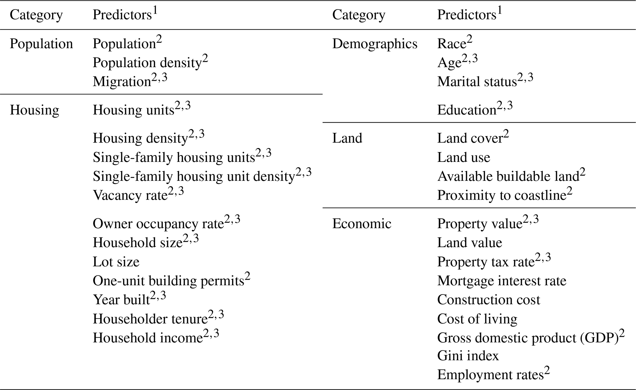
¹ Data sources for all predictors are available in Table S1 (Sect. S1.4). ² Denotes it was considered in the proposed model. ³ Denotes data only available on a decadal basis prior to 2010 (Fig. S1 and Sect. S1.3).

3 Data

Modeling the annual changes in the number of housing units for 1000 counties over a 10-, 20-, or 30-year time horizon requires a dataset of annual county-level data for more than 10 years for all counties in the study area. Counties were chosen as the unit of analysis, as opposed to census tracts, block groups, or a grid analysis, because county boundaries rarely change over a multi-decade period, and data are available at the county-level over multiple decades for most of the predictors in Table 1. Of the 32 predictors identified as potential predictors of new housing construction, 25 (indicated by “²” in Table 1) had county-level data available for more than 10 years and were considered for this study. Data for these 25 predictors were compiled into a dataset for all available years from 1970 on (Sect. S1 in the Supplement). Data for 16 predictors are only available on a decadal basis prior to 2010 (indicated by “³” in Table 1), requiring linear interpolations to provide a consistent annual dataset. Of the 25 predictors considered, 19 have data available starting in 1990 or earlier. Lastly, due to the significant impact of the Great Recession on the nation's housing construction industry, data in 2008, 2009, and 2010 were removed. While the impact of shocks, such as the Great Recession or the COVID-19 pandemic, have caused sizable disruptions to the housing market and should be considered in resiliency planning, the goal of this work is to predict the number of net new housing units under normal conditions. Predicting economic shocks is outside the scope of this work. In total, the individual variables used for this study are available in time intervals from 16 years (2001–2007 and 2011–2019) to 46 years (1971–2007 and 2011–2019) for 1000 counties. For details about the data preprocessing, see Sect. S1.

4 Model types

To estimate the number of new housing units per county over the next 10 to 30 years across a region, a set of time series models and range of model parameters were considered. The time series models tested include a simple linear trend model, ARIMA models, and LSTM neural network models. The ranking criteria for all models compared in this study was prediction performance of the number of housing units for 30 years in the future. Linear trend models were included in the model comparison as a baseline because they are commonly used in forecasting applications, are quick to implement, and are easy to interpret. ARIMA models were tested because they are easy to use, commonly applied across a range of disciplines, and interpretable. LSTM models were considered for their ability to handle large quantities of spatial and temporal data and produce small errors. These three models were ultimately chosen to compare the tradeoffs between model simplicity and model accuracy; if the linear or ARIMA models produce errors in the same range as the LSTM models, then these simpler models may be recommended for housing projections.

4.1 Linear trend

The simple linear trend method consisted of fitting one univariate linear model to each county using ordinary least-squares (OLS) regression (i.e., $y=mx+b$). Each model was fit to the number of housing units, and the resulting trend line was extrapolated to estimate the number of housing units for the following 10, 20, and 30 years.

4.2 Autoregressive integrated moving average (ARIMA)

ARIMA models are univariate linear models that use lagged observations of the time series data and are the most common methods for time series modeling (Box et al., 2016). Equation (1) presents an ARIMA model to predict the value of variable y at time t as a function of values of y at previous time steps ($y_{t-\mathrm{1}},\mathrm{\dots },y_{t-p}$) and error terms at time t and at previous time steps (${\mathit{ϵ}}_t,\mathrm{\dots },{\mathit{ϵ}}_{t-q}$). The parameters $\mathit{\alpha };{\mathit{\beta }}_{\mathrm{1}},\mathrm{\dots },{\mathit{\beta }}_p$; and ${\mathit{\varphi }}_{\mathrm{1}},\mathrm{\dots },{\mathit{\varphi }}_q$ are estimated from the data. ARIMA models are typically referred to by the values p, d, and q, where p is the number of lags for the autoregressive term, d is the number times the data must be differenced to be stationary prior to model fitting, and q is the number of lagged forecast errors for the moving average term. This study also compares the method of using one ARIMA model for all counties in the study area (one set of p, d, and q values) vs. an individual ARIMA model for each county to understand whether a simple uniform ARIMA model could be used across the study region. The annual percent change in number of housing units was used as y in Eq. (1).

$$\begin{array}{}\text{(1)}& \begin{array}{rl}{y}_t& =\mathit{\alpha }+{\mathit{\beta }}_{\mathrm{1}}{y}_{t-\mathrm{1}}+{\mathit{\beta }}_{\mathrm{2}}{y}_{t-\mathrm{2}}+\mathrm{\dots }+{\mathit{\beta }}_p{y}_{t-p}\\ & +{\mathit{\varphi }}_{\mathrm{1}}{\mathit{ϵ}}_{t-\mathrm{1}}+{\mathit{\varphi }}_{\mathrm{2}}{\mathit{ϵ}}_{t-\mathrm{2}}+\mathrm{\dots }+{\mathit{\varphi }}_q{\mathit{ϵ}}_{t-q}+{\mathit{ϵ}}_t\end{array}\end{array}$$

4.3 Long short-term memory (LSTM)

Neural network models have emerged as a common method for analyzing complex problems due to their ability to handle large, nonlinear datasets with high accuracy. Recurrent neural networks (RNNs) are specifically utilized for sequential modeling applications, such as time series forecasting and natural language processing, and can be used to predict future housing inventories given a sequence of variables with nonlinear relationships across a large study area. LSTM models are the most common among the family of RNNs available and were chosen in this study for their ability to learn both long-term and short-term dependencies across a sequence of multivariate input data. The time dependencies are learned in an LSTM unit across a series of LSTM memory cells. Each cell consists of three “gates” that manage the information passed across the sequence of input data. The “input gate” regulates whether to add new information to the memory of the cell; the “forget gate” removes information to be considered in the given memory cell; and the “output gate” regulates the information leaving the cell. For more on LSTM models, see Hochreiter and Schmidhuber (1997), Ienco et al. (2017), and Wang et al. (2020b).

All neural network models, including LSTMs, have a set of hyperparameters that are unique to a given model and are tuned to improve model performance. For LSTM models, tuning parameters include the number of input time steps and output time steps, number of features and targets, number of layers and nodes, activation method, loss metrics, type of optimizer, learning rate, batch size, batch normalization, use of dropouts and dropout rates, and number of epochs. Data are also split into training and testing sets typically using a $\mathrm{70}/\mathrm{30}$ or $\mathrm{80}/\mathrm{20}$ ratio, allowing a model's performance to be evaluated both on the data for which it is developed (the training set) and an independent dataset (the testing set). Lastly, due to variability in each run of the neural network algorithm, a single model configuration is often tested multiple times to search for the model producing the lowest errors.

5 Analyses and evaluation

To identify the best time series model for predicting the number of housing units up to 30 years in the future, a range of model configurations was tested (Table 2). Four sets of feature variables (also known as independent or explanatory variables) and the target variable (also known as the dependent or response variable) for each model were also compared in the analysis (Table 3). The target variable for the linear trend model is h_itk, with the number of housing units for county $i\in (\mathrm{1},\mathrm{\dots },I)$ in year $t\in (\mathrm{1},\mathrm{\dots },T_{\mathrm{o}})$ in sample $k\in (\mathrm{1},\mathrm{\dots },K)$, where a sample k is one sequence of input and output years for county i (Fig. 2). The target variable for remaining models is r_itk, with the annual percent change of the number of housing units for county i in year t in sample k, defined in Eq. (2).

$$\begin{array}{}\text{(2)}& r_{itk}={\displaystyle \frac{h_{itk}-h_{i,t-\mathrm{1},k}}{h_{i,t-\mathrm{1},k}}}\cdot \mathrm{100}\end{array}$$

Table 2 Model tests.

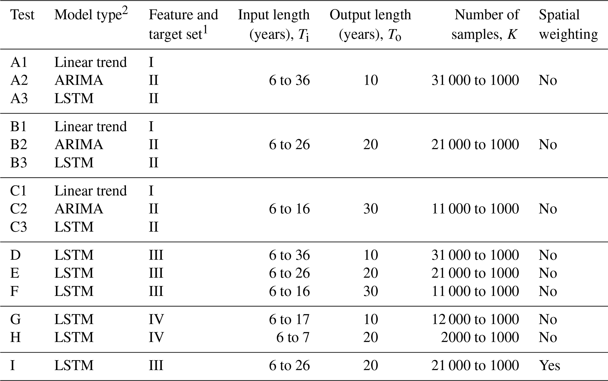
¹ Feature and target sets are defined in Table 3. ² For Tests A3, B3, and C3, for each input–output combination, the best result of five runs was chosen. For Tests D, E, F, G, H, and I, for each input–output combination, the best result of 10 runs was chosen.

Table 3 Feature and target sets.

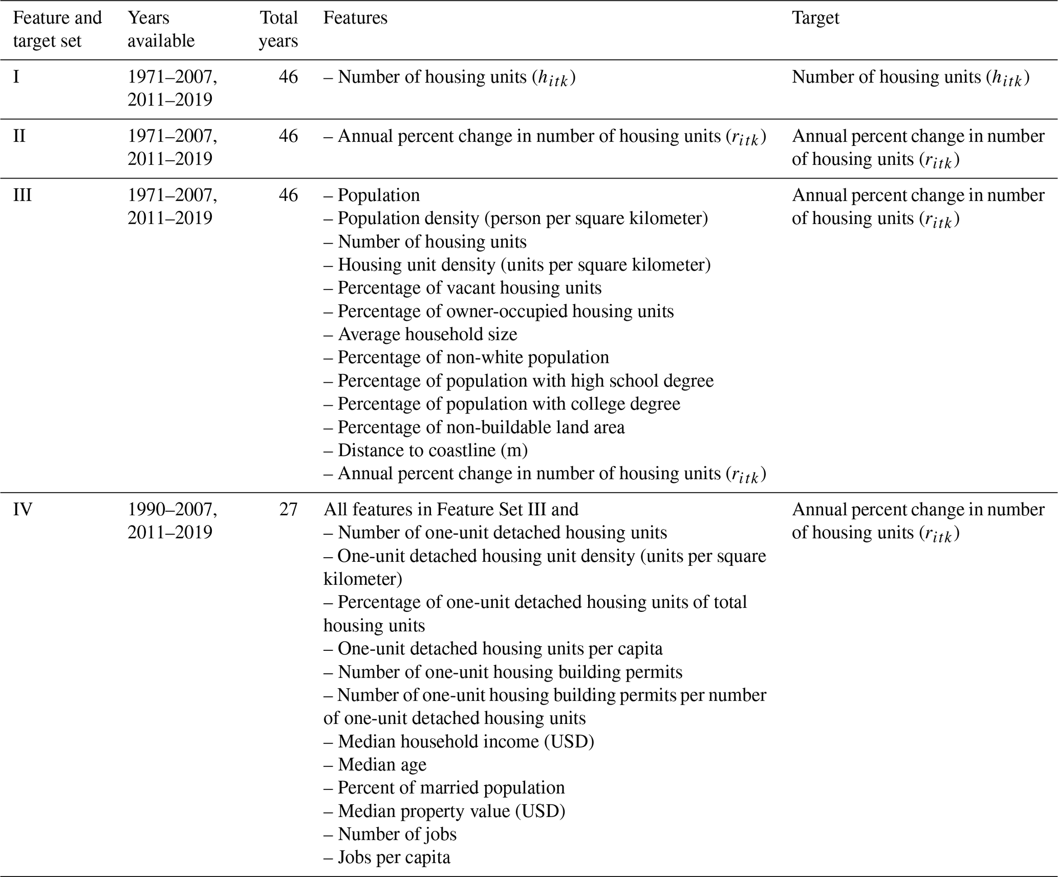
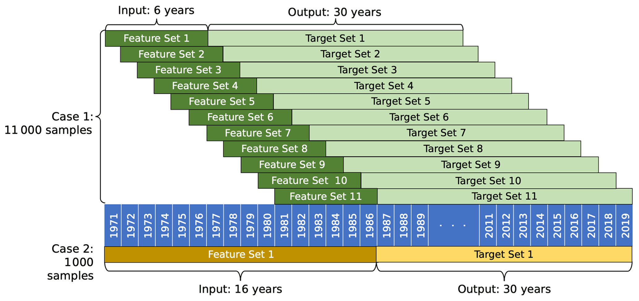
Figure 2 The change in sample size (K) for two different input year lengths (T_i) for Test C1.

The two target variables, h_itk and r_itk, are directly related, but the range of h_itk values for all counties across all available years spans multiple orders of magnitude, from 50 to 1.8 million housing units. The large spread in the data makes it difficult to fit a model across all counties and all years with h_itk as a target variable. The use of r_itk overcomes this problem, with values from −78 % to 132 % annual change in housing units.

Each test predicts values for all 1000 counties over a 10-, 20-, or 30-year time period so that a model with a 30-year projection period, for example, predicts 30 000 unique county-year values. A range of input sequence lengths were compared across all tests to determine the optimal input and output length structure for each model type. The combined input and output lengths determine the total number of samples K used to train and test the model, where a shorter time interval leads to more samples for training and testing a model, while a longer time interval leads to fewer samples for the model. Specifically, when the sum of the input and output length (T_i+T_o) is less than the number of years in the dataset T there are ($T-(T_{\mathrm{i}}+T_{\mathrm{o}})+\mathrm{1}$) samples of data for each county. As an example, say Test C3 was implemented for just one county. Test C3 uses Feature Set I, which has T=46 years of available data and a T_o=30-year output length. For one case evaluated in Test C3 that has an input length of T_i=6 years, the resulting total input–output time interval is 36 years, leading to a total of $\mathrm{46}-(\mathrm{6}+\mathrm{30})+\mathrm{1}=\mathrm{11}$ different time intervals across the 46 years of available data for the single county. For all 1000 counties in the study area, this test configuration would result in K=11 000 samples available to train and test the model (Case 1, Fig. 2). However, if the input length is instead T_i=16 years and the output length is T_o=30 years, the total length of the time interval is 46 years, allowing only $\mathrm{46}-(\mathrm{16}+\mathrm{30})+\mathrm{1}=\mathrm{1}$ sample for a given county and K=1000 samples over the entire study area (Case 2, Fig. 2).

In Tests A, B, and C, the univariate linear trend, ARIMA, and LSTM models were compared to identify the best input–output length combination for each model and the best univariate model performance. Since the linear trend and ARIMA models are restricted to one variable, for fair comparison, the LSTM was similarly restricted in Tests A, B, and C. These tests used data available since 1971, thus providing 46 years of data to fit the model (note that the Great Recession is excluded). For the simple linear trend modeling, each county was fit to an individual linear model, and errors were aggregated across all counties. Similarly, the ARIMA models fit individual ARIMA models for each county for a given p, d, and q combination, and errors were aggregated across all counties. The p, d, and q values tested ranged from 0 to 2. For LSTM models in Tests A, B, and C, the best of five LSTM runs for each input–output combination was taken as the solution.

Tests D, E, and F compared the multivariate LSTM models to identify the best input–output length combination for each model and the best multivariate model performance. These tests only included the 13 feature variables in Feature Set III which were available since 1971 and provided 46 years of available data. LSTM models in Tests D, E, and F recorded the best of 10 LSTM runs.

Tests G and H used LSTM models with 25 feature variables to understand whether more features improve model performance. A tradeoff exists between including more features but having a shorter time span of available data and including fewer features but having a longer time span of available data. Feature Set IV used in Tests G and H is only available since 1990 and provides just 27 years of data. These two tests recorded the best of 10 LSTM runs.

The literature suggests there are both time and space dependencies when modeling housing projections (Cho et al., 2005; Strader et al., 2015); thus Test I reviewed an LSTM model that included spatial weighting across all counties for all features in Feature Set III. With influence from graph neural network methods (Wu et al., 2021), spatial weighting was applied so that feature values in each county were averaged among all contiguous counties prior to model fitting. For example, the population feature variable for a given county would be reassigned as the non-weighted average population value of the county itself and all counties directly adjacent. The values for the remaining feature variables for a given county would then be similarly reassigned. Once spatial weighting was applied to all counties for all feature variables, then the model was fit accordingly. No spatial weighting was applied to the target variable, and this test recorded the best of 10 LSTM runs.

For all LSTM models in Tests A through I, samples were randomly divided for a given input–output combination into a training and testing set using an $\mathrm{80}/\mathrm{20}$ split. As a result, the set of samples for a given county were randomly distributed into the training and testing sets. Holdout validation was not implemented in this study because the developed model is not intended for use outside the defined study area of 1000 counties. Both training and testing errors are tracked to identify possible overfitting. The same hyperparameters were used in all LSTM models (Table S2 and Sect. S2.3.2).

All models were evaluated using the root mean squared error RMSE_r of the annual percent change of housing units (Eq. 3), as well as the expected value $E\left[\right|H\left|\right]$ and standard deviation $s_{\left|H\right|}$, over all I, T_o, and K values of the absolute value of the percent relative error in number of housing units H_itk (Eq. 4), where ${\widehat{r}}_{itk}$ is the predicted annual percent change of housing units in county i, year t, and sample k; r_itk is the observed annual percent change of housing units; ${\widehat{h}}_{itk}$ is the predicted number of housing units; h_ikt is the number of observed housing units; and I, T_o, and K are the numbers of counties, number of years in the output series, and number of samples, respectively.

$$\begin{array}{}\text{(3)}& {\displaystyle }{\text{RMSE}}_r=\sqrt{{\displaystyle \frac{{\sum }_{ikt}({\widehat{r}}_{itk}-r_{itk}{)}^{\mathrm{2}}}{I{T}_{\mathrm{o}}K}}}\text{(4)}& {\displaystyle }{H}_{itk}={\displaystyle \frac{{\widehat{h}}_{itk}-h_{itk}}{h_{itk}}}\cdot \mathrm{100}\end{array}$$

The RMSE_r is based on the target value optimized by the LSTM and the response variable for the ARIMA r_itk; $E\left[\right|H\left|\right]$ and $s_{\left|H\right|}$ are included because they are based on the more easily interpreted variable h_itk. The linear trend and ARIMA models do not separate the data into a training and testing set; therefore the errors were calculated across all output years in all samples. Of the multiple input–output lengths evaluated for each test and the multiple runs for the LSTM models, the input–output combination with the lowest average of RMSE_r, $E\left[\right|H\left|\right]$, and $s_{\left|H\right|}$ values for each test is reported. For example, in Test A3, where 6 to 36 input years were evaluated and the output length was 10 years, there were $\mathrm{36}-\mathrm{6}+\mathrm{1}=\mathrm{31}$ different models evaluated, each over five runs. Of those $\mathrm{31}\cdot \mathrm{5}=\mathrm{155}$ models, the model with the lowest average RMSE_r, $E\left[\right|H\left|\right]$, and $s_{\left|H\right|}$ value was reported as the best model for Test A3.

Each time series model was fitted and evaluated using a publicly available Python (Van Rossum and Drake, 2009) library: the scikit-learn package for the linear trend model (Buitinck et al., 2011), the statsmodel package for ARIMA (Seabold and Perktold, 2010), and the TensorFlow package for LSTM models (Abadi et al., 2015).

6 Results

6.1 Model comparison

6.1.1 Model type comparison

We first compare the model types. For the univariate models evaluated in Tests A, B, and C, the LSTM method outperforms the simple linear trend and ARIMA models for 10-, 20-, and 30-year prediction periods (Table 4). For the 30-year prediction period, for example, the linear trend, ARIMA, and LSTM models have RMSE_r values of 2.0, 1.8, and 1.2, respectively, and $E\left[\right|H\left|\right]$ values of 11.4, 12.7, and 0.64, respectively (Table 4, Tests C1, C2, and C3).

Table 4 Results.

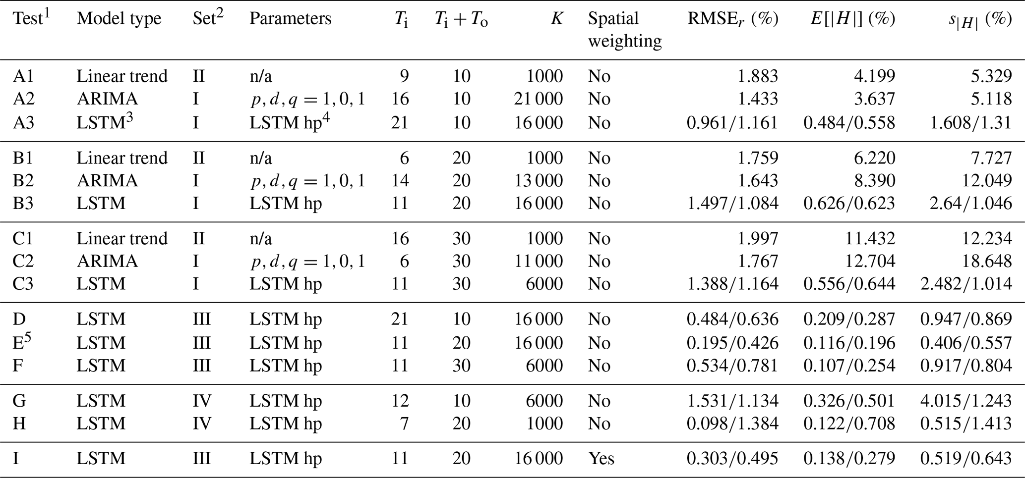
¹ Of the multiple input–output lengths evaluated for each test and the multiple runs for the LSTM models, the input–output combination with the lowest average of RMSE_r, $E\left[\right|H\left|\right]$, and $s_{\left|H\right|}$ values for each test is reported. ² Feature and target sets are defined in Table 3. ³ All LSTM models report training errors and testing errors. ⁴ See Table S2 for a list of the hyperparameters (hp) used for all LSTM models. ⁵ Recommended REACH20 model. n/a stands for not available.

Comparing the linear trend and ARIMA models, the best model type depends on the metric used and output length. In terms of RMSE_r, the ARIMA model performs better than linear trend models for all output lengths. In terms of $E\left[\right|H\left|\right]$, however, the linear trend model is 2.17 and 1.27 percentage points better than the ARIMA model for 20- and 30-year output lengths, respectively. The error distribution for the linear trend and ARIMA models are nearly the same (Fig. 3a, b, and c). Therefore, when quick long-term projections are needed, a simple linear trend model method may be adequate. The distribution of the testing errors for the LSTM model is much smaller than for linear trend and ARIMA models, and all output lengths have a similar distribution (Fig. 3d).

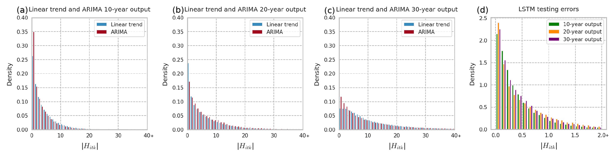
Figure 3 Absolute percent relative error ($|H{|}_{itk}$) distributions for univariate models. (a) Linear trend vs. ARIMA 10-year output. (b) Linear trend vs. ARIMA 20-year output. (c) Linear trend vs. ARIMA 30-year output. (d) LSTM for all output lengths (note that the x-axis scale for d differs from the others).

6.1.2 Input and output lengths

A key issue in fitting these models is determining the best number of years of input and output data to use. The number of years of output T_o will depend in general on the intended use of the model, although it may be important to understand the tradeoff between forecasting for a longer duration into the future and keeping errors lower in case there is flexibility on the required output length. The results suggest that, as expected, errors in terms of $E\left[\right|H\left|\right]$ are larger for longer output lengths (Tests A, B, and C, Table 4). That is, it is easier to forecast the number of housing units accurately for 10 years than for 20 years and easier to forecast for 20 years than for 30 years. For errors in terms of RMSE_r, the pattern is similar, though not as consistent.

For a specified desired output length, the optimal number of years of input is not obvious a priori, as it depends on data availability and the extent to which variable values from previous years help predict target variable values in future years. If the value of a variable x in each year t is related to that in the preceding year t−1, then x_t−2 has an implicit indirect effect on x_t as well, through x_t−1. Thus, it may be that including data for x from many input years helps predict x_t, but it may not be required and could just add noise. The housing vacancy rate in 1970 may not be relevant to the change in the number of housing units from 2020 to 2021, for example, beyond the indirect influence it has on the changes in the intervening years. The input length also affects the total number of samples available to fit a model, where there is a tradeoff between a longer input length and fewer total samples vs. a shorter input length with more training samples (Fig. 2).

The best-performing linear trend models all had input sequence lengths shorter than the output sequence lengths. With 46 years of data total, when the output length is 10 years, for example, the maximum input length is 36 years, but the best linear trend model had an input length of 9 years (Table 4, Test A1).

For the ARIMA models, shorter input lengths performed better, where 16, 14, and 6 years were identified as the best input lengths corresponding to 10, 20, and 30 years of output (corresponding to 21 000, 13 000, and 11 000 available samples, respectively). Additionally, for all output lengths, the best p, d, and q values tested were 1, 0, and 1, respectively, suggesting that just one lag of the autoregressive term, one lag of error terms, and no differencing for the annual percent change of housing units data can be used for quick and approximate housing forecasts.

The univariate and multivariate LSTM models have the same best input length for a given output length, where the best input lengths include the years in either 1 decade (11 years inclusive) or 2 decades (21 years inclusive). This could result from the nature of the data availability, where most variables are only available at a decadal scale prior to 2010 (Fig. S1 in the Supplement and Sect. 1.3).

6.1.3 LSTM model comparisons

Focusing on the LSTM models, which offer the smallest errors, we investigate feature selection, spatial weighting, and possible overfitting. To determine if additional feature variables help forecast the number of housing units in each county, we compare models that are the same except for the feature set. Tests A3, B3, and C3 use Feature Set I (only the target variable); Tests D, E, and F use Feature Set III (13 feature variables); and Tests G and H use Feature Set IV (with another 12 additional feature variables) (Table 3). The multivariate LSTM models in Tests D, E, and F outperform the univariate LSTM models evaluated in Tests A, B, and, C on all metrics and for all output lengths, where the errors from the multivariate model are approximately half those from the univariate model (Table 4). This suggests that the feature variables in Feature Set III do substantially improve prediction of future numbers of housing units. Comparing Tests D and E to Tests G and H, however, indicates that incorporating the additional 12 feature variables of Feature Set IV does not improve prediction. Since data are only available since 1990 for variables in Feature Set IV, there is a tradeoff between adding the features and maximizing the duration of data availability, and the results suggest incorporating the additional features does not add value to the modeling.

Of all the LSTM models evaluated in Tests A through H, the best-performing model is Test E, a multivariate LSTM having 11 input years and 20 output years with 13 features of data that are available since 1971. When, in Test I, spatial weighting was added to the features for the same 11-year input, 20-year output model, there was no substantial improvement in errors. The test data $E\left[\right|H\left|\right]$ for Tests E (without spatial weighting) and I (with spatial weighting) are 0.196 and 0.279, respectively.

Finally, comparing the testing and training errors for all LSTM models and both RMSE_r and $E\left[\right|H\left|\right]$ does not suggest a substantial overfitting or underfitting problem. Across the nine LSTM models, the median value of the ratio ${\text{RMSE}}_r\text{(testing)}/{\text{RMSE}}_r\text{(training)}$ is 1.71, and the median of $E\left[\right|H\left|\right]\text{(testing)}/E\left[\right|H\left|\right]\text{(training)}$ is 1.54.

Based on all the results in Table 4, the best LSTM model in Test E is considered the recommended model to predict the number of housing units h_itk for the 1000 counties in the study area over a 20-year period. This model is henceforth referred as the 20-Year Regional Annual County-Level Housing (REACH20) model. If an application required a 30-year prediction period, the best LSTM model in Test F, with 11 input years and 30 output years, would be recommended.

6.2 Evaluation of the recommended LSTM model

This section evaluates the recommended 11-year input and 20-year output multivariate LSTM REACH20 model in more detail, examining the magnitude and distribution of errors. The REACH20 model has an expected absolute percent relative error ($E\left[\right|H\left|\right]$) for the testing set of less than 0.2 % when comparing the predicted number of housing units h_itk with the observed number of housing units ${\widehat{h}}_{itk}$. That means, on average, across all predicted years t∈T_o, samples k, and counties i, the number of housing units predicted differs from the actual number of housing units by less than 0.2 %, likely negligible for many applications. Additionally, of the 64 000 predicted data points in the testing set (3200 samples in the testing set (16 000⋅0.2) and 20 predicted years), almost all (97.3 %) had absolute percent relative errors of less than 1 % ($\left|H_{itk}\right|<\mathrm{1.0}$). The distribution of the relative errors among the predicted data points has essentially no bias and an even balance of over- and underprediction (Fig. 4a).

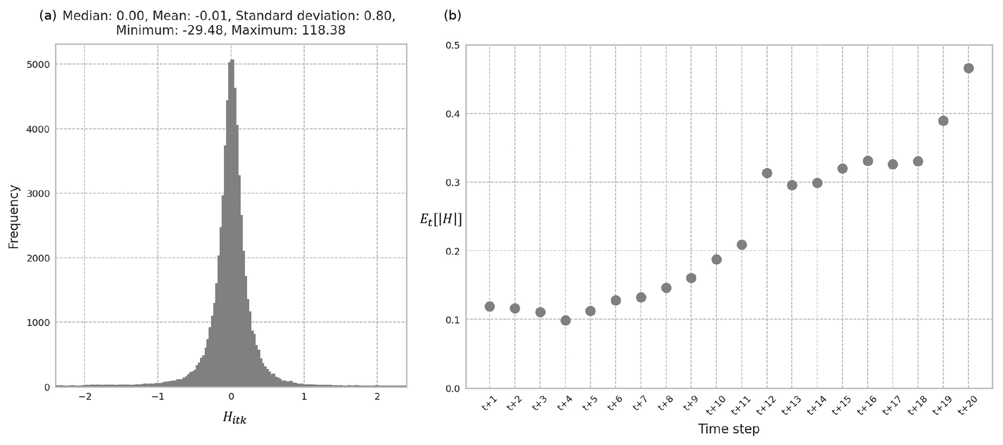
Figure 4 (a) Distribution of H_itk of the testing set using the REACH20 model. (b) Average absolute percent relative error for each time step over all counties and samples $E_t\left[\right|H\left|\right]$ for the testing set using the REACH20 model.

When reviewing the variability of the testing set errors over the duration of the 20-year prediction period, the expected value $E_t\left[\right|H\left|\right]$ over all counties i and samples k of the absolute value of the percent relative error for each time step t for the testing set remains under 0.5 %. There is a noticeable, gradual increase in the errors as the predicted year horizon expands. The $E_t\left[\right|H\left|\right]$ value, for example, is 0.12 % in the first time step and 0.47 % in the 20th time step (Fig. 4b). This suggests that while the errors are quite low for all years in the 20-year prediction period, the model does not predict the number of housing units 20 years in the future as well as it does the number of housing units 1 to 5 years in the future, as expected. Furthermore, the population projection method provided by Hauer (2019) for all US counties produce aggregated relative errors of 0.9 % to 3.6 % over a 15-year projection period, while the recommended model in this study produces average absolute relative errors of less than 0.5 % over a 20-year projection period. This suggests that if a static housing unit per population ratio was applied to the population estimates produced by Hauer (2019), as is done in other studies evaluating natural hazard risk in the context of a changing housing inventory (Hauer et al., 2016; Ashley and Strader, 2016; Strader et al., 2015, 2018; Freeman and Ashley, 2017; Sleeter et al., 2017; Davidson and Rivera, 2003), these housing estimates would likely be less accurate than those produced by the recommended REACH20 model.

Errors across space were also reviewed to understand whether the model performs better for certain geographic areas (e.g., urban vs. rural counties or East Coast vs. Gulf Coast). There is no obvious spatial pattern of the expected value $E_{\mathrm{i}}\left[\right|H\left|\right]$ across the study area, with a balance of overprediction (purple) and underprediction (green) across the region (Fig. 5). There were 987 counties (98.7 %) with averaged H_itk across all time steps less than 0.2 %. Errors in western Texas are slightly larger than other regions of the study area perhaps due to the relatively small population of these counties and the associated sensitivities to small changes in the error.

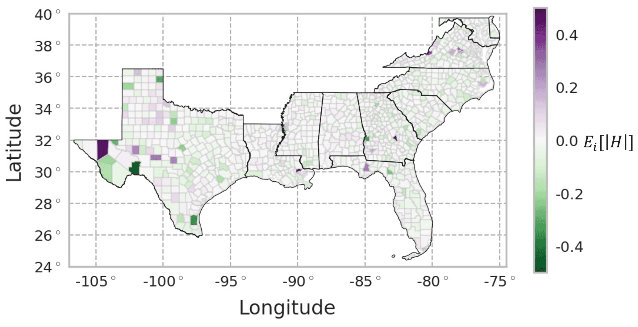
Figure 5 Average percent relative error for each county over all predicted time steps and samples, $E_i\left[\right|H\left|\right]$, for the combined training and testing set using the REACH20 model. Given that the samples for a given county and time sequence were randomly split into the training and testing set, a spatially complete view of the errors required a combination of the training and testing errors.

6.3 Implications of projected change in housing inventory

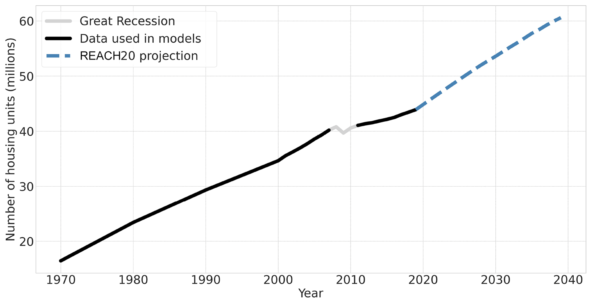
Over the entire study region, the REACH20 model predicts approximately 16.7 million more homes in the 20-year forecast period between 2019 and 2039 (38 % growth, Fig. 6). The aggregated county-level projections are based on the last 11 years of available data excluding the Great Recession (2006, 2007, and 2011–2019) for the 13 included features to estimate 20 years of future housing unit projections across all 1000 counties using the REACH20 model.

Figure 6 Predicted number of housing units in the study area using the REACH20 model.

The projected housing rates of change across all counties over 20 years (2019–2039) vary spatially, where the housing inventory in almost all counties (97.4 %) is expected to grow over the next 20 years (Fig. 7). Suburban and exurban counties are projected to have large housing growth rates over the next 20 years, which is reasonable, as urbanization in metro areas continues. There are noticeable differences in projected housing rates within the state of Texas. In the eastern half of the state, there is large projected growth around the state's major cities which aligns with recent trends; 6 of the 15 fastest-growing large cities in the US between 2010 and 2019 are located in Texas (US Census Bureau, 2020b). However, housing inventory is projected to generally remain stagnant or decline in western Texas, which aligns with past trends of the generally stagnant population and available jobs in the region (Texas Comptroller, 2020).

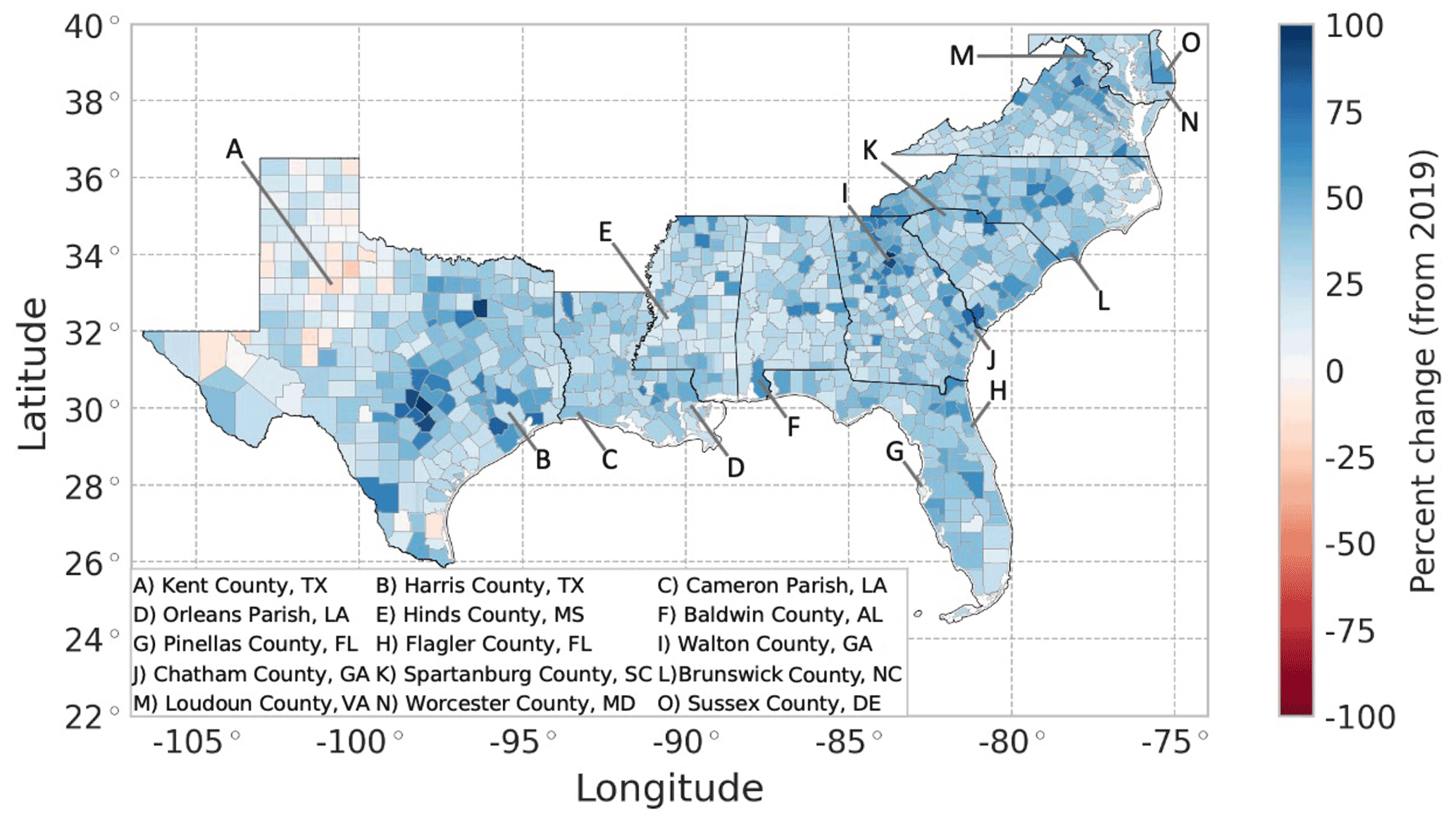
Figure 7 Projected 20-year (2019–2039) percent change in housing units using the REACH20 model. The blue color represents growth, and red represents decline.

A comparison of the housing rates of change in the past 20 years (1999–2019) vs. the next 20 years (2019–2039) allows for an analysis of housing growth acceleration or deceleration (Fig. 8). The vast majority of counties (89.5 %) in the study area are expected to experience greater housing growth rates in the next 20 years (2019–2039) than in the past 20 years (1999–2039). These higher growth rates indicate that most counties need to carefully manage the rapid new home construction. Additionally, three out of four (75.4 %) counties in the region are expected to experience at least a 10 % change in housing rates in the projected 20 years vs. the past 20 years. Two out of five counties (38.2 %) in the region are expected to experience at least a 20 % change in housing rates between the two periods. This means that a simple linear extrapolation from the past 20 years will likely not provide an accurate projection of housing units.

Figure 8 Projected 20-year housing acceleration (projected percent change in housing units between 2019 and 2039, minus the percent change of housing units between 1999 and 2019) using the REACH20 model. The green color represents an acceleration, and pink represents a deceleration.

A change in housing units over time also implies a change in housing density over time, often resulting in increased urbanization within a county (Fig. 9). Most counties (71.4 %) are only expected to see a change of 10 housing units per square kilometer or less in the next 20 years. However, one-fifth of the counties (21.2 %) in the region are expected to experience an increase of 10 to 50 housing units per square kilometer, many of which are located along the Atlantic coast. Notably, the vast majority of the counties along Florida's coastline (74.5 %) are expected to experience an increase of 10 to 100 housing units per square kilometer. Of the coastal counties, Harris County is expected to experience the greatest increase in housing density, from 400 housing units per square kilometer in 2019 to 510 housing units per square kilometer in 2039. Areas of high density allow for the possibility of more homes being affected by a single hurricane or other hazard event.

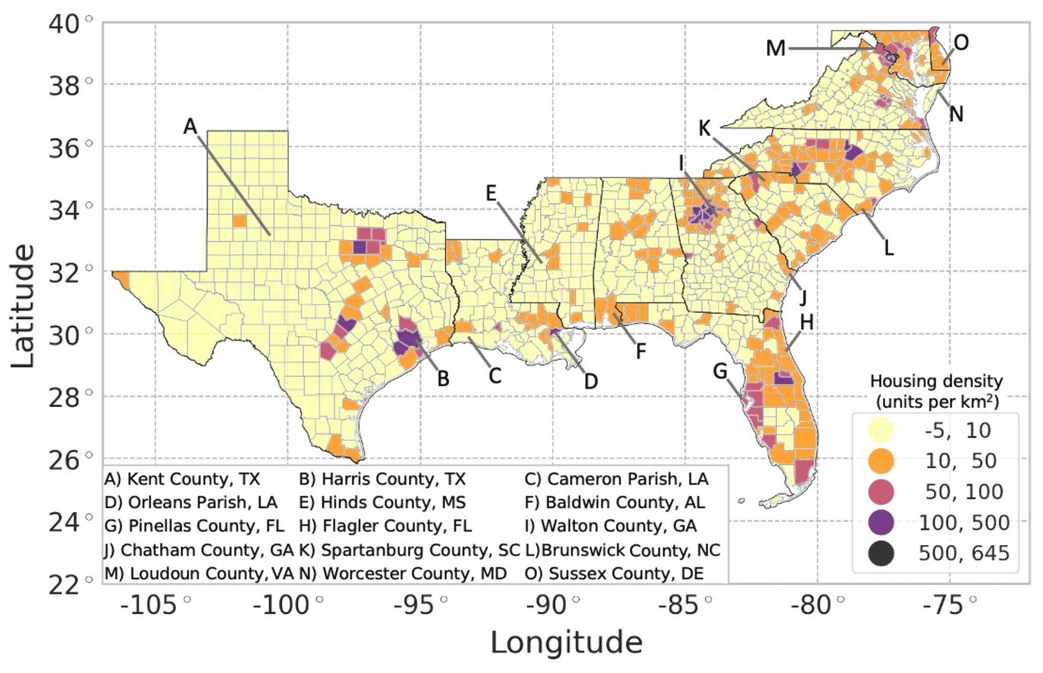
Figure 9 Projected 20-year change in housing unit density (2039 housing unit density minus 2019 housing unit density) using the REACH20 model (units per square kilometer).

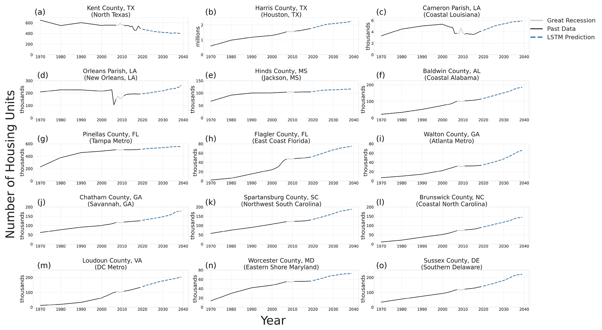
Figure 10 Past and projected number of housing units for 15 counties using the REACH20 model (note the different scales).

To investigate the projected number of housing units in more detail, a sample of 15 counties is identified (Figs. 7–10). The 15 counties selected, which include 1 or 2 from each state in the study area (excluding Washington, DC) and 10 on the coast in hurricane-prone areas, were selected to illustrate some of the variability across counties. In five of the sampled counties (Kent County, Texas; Harris County, Texas; Flagler County, Texas; Brunswick County, North Carolina; and Loudoun County, Virginia), the future housing trend (growing or shrinking) is expected to decelerate over the next 20 years, compared to the last 20 years. The two Louisiana parishes sampled (Fig. 10c), Cameron Parish and Orleans Parish (Fig. 10d), however, are examples of exceptions that experienced significant shocks in the housing inventory due to hurricane impacts.

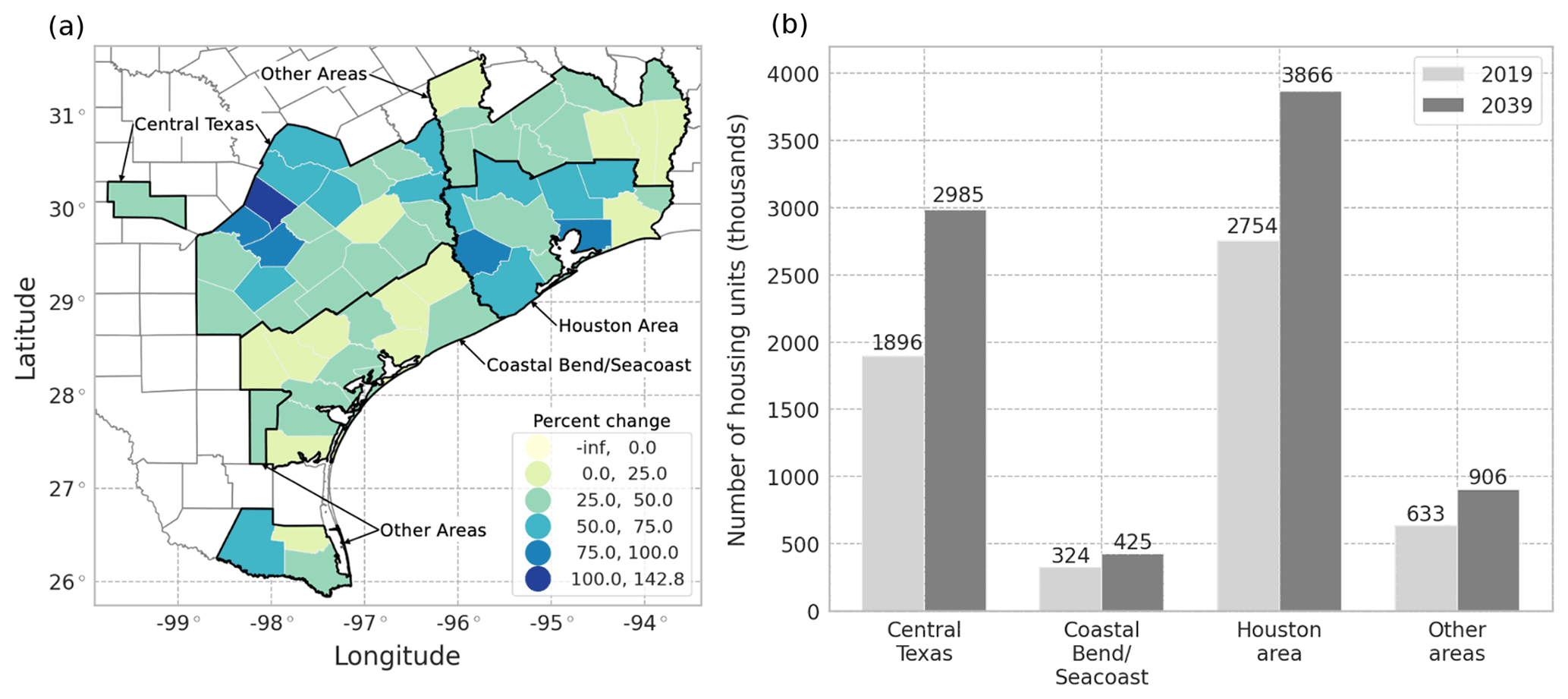
Figure 11 (a) Projected 20-year (2019–2039) percent change in housing units in the Hurricane Harvey-affected region using the REACH20 model. (b) Projected housing units and housing growth rates for the Hurricane Harvey-affected region using the REACH20 model.

6.4 Implications for hurricane impacts and losses

The dynamics of the housing inventory also causes changes in a region's level of risk for multiple hazards, including hurricanes. Hurricane Harvey was a devastating Category 4 hurricane that made landfall on the Texas coast on 25 August 2017, affecting many counties in southeastern Texas. Coastal counties experienced 130 mph (209 km h⁻¹) winds, heavy rains, and large storm surges, while inland counties, particularly in the Houston, Texas, area, experienced massive amounts of rain over multiple days. Across the 62 counties affected by Hurricane Harvey in Texas, there was USD 2.4 billion in residential property losses and USD 7.5 billion in flood insurance losses (Texas Department of Insurance, 2019). Using the proposed REACH20 model, if a hurricane of a magnitude similar to Harvey hit that same Texas region 20 years from now, assuming the same 2017 distributed hazard and vulnerability profiles of newly built homes, the residential property losses for the entire region would be USD 3.2 billion, which is USD 792 million (or 33 %) greater than the damage caused by Hurricane Harvey in 2017, assuming constant dollars. The total flood losses for the region would be even larger, totaling to USD 10.4 billion, which is approximately USD 3 billion (or 40 %) greater than Hurricane Harvey losses.

A closer examination of the projected housing growth rates across the subregions affected by Hurricane Harvey reveals that each subregion would experience a different magnitude of losses. The subregions analyzed align with the four areas identified by the Texas Department of Insurance (2019) report, which documents insurance claims and losses from Hurricane Harvey in the state of Texas. Using the recommended REACH20 model, it is expected that the projected 20-year housing growth rates for each county in these areas will vary over the region (Fig. 11a), and the number of housing units will increase in each subregion (Fig. 11b).

The area identified as the Coastal Bend and Seacoast counties experienced the brunt of the wind force from Hurricane Harvey and accounted for the largest residential property losses (USD 1.4 billion). Residential property losses account for the majority of damages due to high winds and include claims from homeowner's insurance, mobile homeowner's insurance, and residential dwelling insurance. The Coastal Bend area is expected to have the lowest housing growth rate of the region (31.0 % or approximately 100 000 more housing units), yet a similar-sized storm event hitting the same area in 20 years would result in an estimated USD 431 million more in losses than experienced in 2017, assuming constant dollars (Fig. 12a).

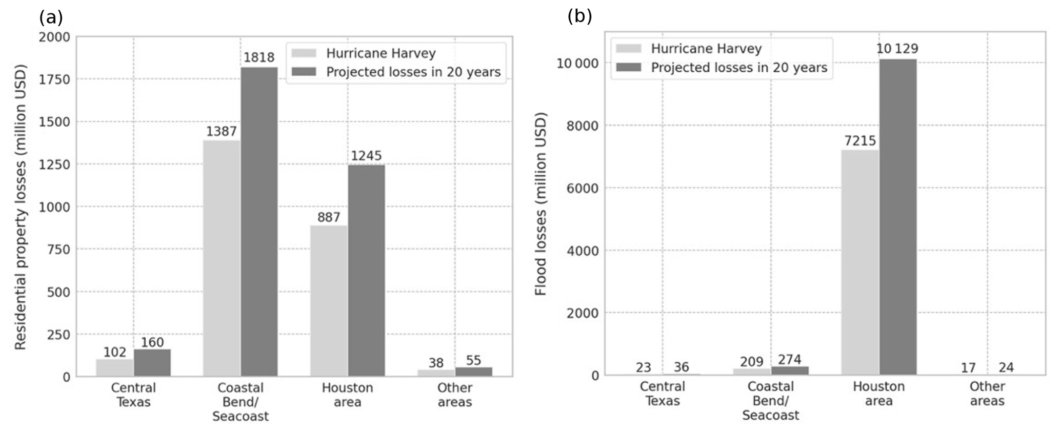
Figure 12 (a) Estimated residential property loss due to hurricane impact across the Hurricane Harvey-affected region over a 20-year period, assuming constant dollars. (b) Estimated flood loss due to hurricane impact across the Hurricane Harvey-affected region over a 20-year period, assuming constant dollars. These values are calculated by multiplying the loss values from Hurricane Harvey in each subregion by the expected 20-year housing growth rate for each subregion.

The area identified as the Houston area and southeastern Texas experienced a massive amount of rainfall from Hurricane Harvey and accounted for the largest flood losses compared to other subregions (USD 7.2 billion). The flood insurance losses reported are caused by rising water or flood damages in residential or commercial structures and include properties with both federal and private flood insurance. The majority of flood insurance claims were for residential structures under the National Flood Insurance Program (NFIP). The Houston area is expected to have a sizable housing growth rate of 40.0 %, equating to 1.1 million more housing units, over the next 20 years, which would cause a significant increase in expected flood losses for a similar-sized hurricane (USD 2.9 billion, Fig. 12b).

7 Future work and conclusions

7.1 Limitations and future work

The recommended REACH20 model provides a first-of-its kind dataset of annual projected housing inventories for a multi-state region over a 20-year period that can be used to enhance hurricane risk models. Given the nature of the available data and complexity of the modeling method, there are limitations to note. For periods when data were only available at a decadal scale for certain variables, linear interpolations were made to produce an annualized dataset which could have introduced errors to the projection of housing units. Additionally, the data during the Great Recession (2008–2010) were removed because the model can neither predict nor account for large, unexpected exogenous shocks to the residential housing market. Additionally, the projected changes in housing units ultimately assume that past housing development behavior will carry into the future. However, housing demands have changed since the start of the COVID-19 pandemic, and it is unclear how these changes are likely to affect future housing development trends. Climate change may also drive new behaviors in housing development patterns as risks due to sea level rise, intense storm events, wildfires, and excessive heat continue to increase. This study also had counties included in both the training and testing set because the model is only intended to be used for the designated study area. If the model were to be applied outside the study area, a review of holdout validation errors would be required. Lastly, neural network methods require a certain level of expertise and significant effort to gather and standardize large quantities of data. Therefore, for applications only requiring quick estimates for changes in housing units, a simpler linear trend or ARIMA model may be adequate.

There is an opportunity to extend the housing unit projection work and estimate the likely distribution of housing unit types (e.g., single-family, multi-family, or manufactured homes) in each county in the future. Researchers can also extend this work by estimating the likely location of the projected housing units within a given county, which would allow for a more granular estimate of hurricane impacts in a region. Additionally, researchers can evaluate potential policy mechanisms that can minimize the hurricane risk for a region while also incorporating the ever-changing housing growth over time. Lastly, the provided housing unit projections can be applied to a variety of applications, including hurricane evacuation planning, hurricane risk mitigation, or general regional planning activities.

7.2 Conclusions

The recommended REACH20 model advances the field of hurricane risk modeling by producing the first known dataset of county-level annual housing inventory projections over a multi-decade period and multi-state region. It allows a dynamic building inventory to be included in hurricane risk models rather than using the conventional assumption of a static building inventory, thereby producing more realistic regional loss estimates. Additionally, the REACH20 model uses publicly available housing and demographic data and can therefore be easily applied to other regions of interest (see Sect. S2.3 for source code).

LSTM models outperformed linear trend and ARIMA models on all metrics; and the multivariate LSTM models outperformed the univariate LSTM models, although when the inclusion of additional feature variables meant fewer years of available data, they did not lead to improved model performance. Applying spatial weighting by averaging a county's feature values with adjacent counties did not improve model results either. The REACH20 model includes 11 years of input data, 20 years of output data, 13 feature variables, and a single target variable for 1000 counties in the southeastern US over 46 years of available data, resulting in 16 000 samples available to train and test the LSTM model. Using an $\mathrm{80}/\mathrm{20}$ split of training to testing, the 64 000 predicted data points in the testing set (3200 samples in the testing set (16 000⋅0.2) and 20 predicted years), almost all (97.3 %) had absolute percent relative errors of less than 1 % ($\left|H_{itk}\right|<\mathrm{1.0}$), meaning the estimated number of housing units was no more than 1 % different than the actual number, which are errors that are acceptable for most practical purposes. The $\stackrel{\mathrm{‾}}{H}$ remained less than 0.5 % for all 20 predicted time steps, and errors were distributed evenly across the study region.

The REACH20 model suggests there will be significant increases in the housing inventories of the southeastern US, thus increased expected hurricane losses. Of the 1000 counties in the study area, 974 are expected to experience a growth in their housing inventory, and 895 counties are expected to have greater housing growth in the next 20 years compared to the past 20 years. Translating this to potential hurricane losses, if a Hurricane Harvey type event hit southeastern Texas in 20 years, losses could increase by approximately 40 %, compared to the losses caused by Hurricane Harvey in 2017. Recognizing the great expected hurricane losses, planners should prioritize mitigation and adaptation measures in the areas with high expected housing growth, thereby decreasing future societal impacts and financial losses.