The influence of infragravity waves on the safety of coastal defences: a case study of the Dutch Wadden Sea

Many coastlines around the world are protected by dikes with shallow foreshores (e.g. salt marshes and mudflats) that attenuate storm waves and are expected to reduce the likelihood and volume of waves overtopping the dikes behind them. However, most of the studies to date that assessed their effectiveness have excluded the influence of infragravity (IG) waves, which often dominate in shallow water. Here, we propose a modular and adaptable framework to estimate the probability of coastal dike failure by overtopping waves (P_f). The influence of IG waves on overtopping is included using an empirical approach, which is first validated against observations made during two recent storms (2015 and 2017). The framework is then applied to compare the P_f values of the dikes along the Dutch Wadden Sea coast with and without the influence of IG waves. Findings show that including IG waves results in 1.1 to 1.6 times higher P_f values, suggesting that safety is overestimated when they are neglected. This increase is attributed to the influence of the IG waves on the design wave period and, to a lesser extent, the wave height at the dike toe. The spatial variation in this effect, observed for the case considered, highlights its dependence on local conditions – with IG waves showing greater influence at locations with larger offshore waves, such as those behind tidal inlets, and shallower water depths. Finally, the change in P_f due to the IG waves varied significantly depending on the empirical wave overtopping model selected, emphasizing the importance of tools developed specifically for shallow foreshore environments.

1 Introduction

1.1 Background

Coastal defences (e.g. dikes or seawalls), fronted by wide, shallow foreshores, protect many coastlines around the world. Examples include the sandy foreshores along the Belgian coast (Altomare et al., 2016); the wide shelves of the Mekong Delta, Vietnam (Nguyen et al., 2020); and the intertidal flats of the Wadden Sea along the northern coast of the Netherlands (Vuik et al., 2016). These bodies of sediment reduce the water depth in front of the structure such that large incident waves are forced to break. The foreshore contributes to a reduced wave load at the structure and is therefore expected to reduce the likelihood of failure. If vegetation is present, the drag forces exerted by stems, branches and leaves further enhance this attenuation effect (Dalrymple et al., 1984; Mendez and Losada, 2004). Several studies sought to quantify the hazard mitigation potential of shallow foreshores, with and without vegetation, including physical model tests (Möller et al., 2014), numerical simulations (Vuik et al., 2016; Willemsen et al., 2020) and field measurements (Garzon et al., 2019). While these studies assessed the ability of the foreshore to attenuate the height of wind-sea and swell (hereafter, SS) waves – with frequencies typically greater than 0.05 Hz – they neglected the influence of infragravity (hereafter, IG) waves.

Under extreme conditions, with large offshore waves and very shallow local water depths, the shoaling and subsequent breaking of SS waves results in energy transfer to lower frequencies and the growth of IG waves, also referred to in literature as “surf beat” (Bertin et al., 2018; Van Dongeren et al., 2016). IG waves are widely recognized as the driving force behind coastal erosion and flooding along shallow coastlines. Recent reports of their impact include the following: unexpectedly high wave run-up at the coast of the island of Bannec, France (Sheremet et al., 2014); extensive damage and casualties along the coral-reef-lined coast in the Philippines during Typhoon Haiyan (Roeber and Bricker, 2015); the erosion and overwash of several dunes along the western coast of France (Baumann et al., 2017; Lashley et al., 2019); and damage along the Seisho coast of Japan during Typhoon Lan (Matsuba et al., 2020). Despite this knowledge, IG waves are often not considered in the risk assessment of coastal defences. This oversight is linked to the common practice where phase-averaged wave models are used to estimate wave parameters at the toe of the structure. These parameters are then used as input to empirical formulae (EurOtop, 2018). As phase-averaged models (e.g. Simulating Waves Nearshore, SWAN; Booij et al., 1999) tend to exclude IG-wave dynamics, the impact of IG waves on the safety of coastal defences is naturally not considered. An empirical approach developed for shallow foreshores using offshore forcing parameters would implicitly account for the intermediate processes, including the effects of IG waves (Mase et al., 2013; Goda, 2010). However, the more widely used formulae are based on parameters at the structure toe (EurOtop, 2018).

In the Netherlands, coastal defences are typically designed to resist the volume of water expected to pass over the crest of (or overtop) the structure due to wave action during storms associated with a very high return period (e.g. 2000 to 10 000 years). This phenomenon, referred to as wave overtopping, is typically represented by a mean (time-averaged) discharge per metre width of structure, q (m³ s⁻¹ m⁻¹ or L s⁻¹ m⁻¹). The probability of failure due to wave overtopping is then determined by assessing the likelihood that the actual discharge (q_a) exceeds some critical value (q_c), which is dependent on the erosion resistance of the grass-covered landward slope. Following a recent policy revision, the safety standard for the coastal defences in the Netherlands is now defined by an (acceptable) probability of failure. For example, typical values for the Dutch Wadden Sea coast – a shallow, intertidal area in the north of the country – are failure probabilities of $\mathrm{1}/\mathrm{1000}$ and $\mathrm{1}/\mathrm{3000}$ per year. This approach usually considers multiple failure mechanisms (e.g. scour, armour unit instability and slope instability); however, here we limit the analysis to dike failure by wave overtopping, which typically governs the design process.

From a design perspective, the presence of IG waves typically results in higher characteristic values of the two main parameters used to estimate q_a: namely, the significant wave height and spectral wave period, both assessed at the structure toe (Van Gent, 1999; Hofland et al., 2017). Vuik et al. (2018b) assessed the overtopping failure probability of an idealized the dike–foreshore system, representative of the Dutch Wadden Sea coast, considering the effects of vegetation. This study considered the influence of IG waves on the wave period at the toe using the Hofland et al. (2017) empirical model but neglected their influence on the wave height. Furthermore, Nguyen et al. (2020) later showed that the Hofland et al. (2017) formulae tend to underestimate the development of longer spectral wave periods on foreshore slopes milder than 1:250 (Nguyen et al., 2020) – which is a typical characteristic of the Wadden Sea. As a result, the true influence of IG waves along the Dutch Wadden Sea coast remains unknown.

Oosterlo et al. (2018) carried out a similar probabilistic assessment of a dike with a sandy foreshore, in the south of the Netherlands, but directly included the IG waves using the XBeach Surfbeat numerical model (Roelvink et al., 2009) to estimate the wave parameters at the toe. The authors found, for the considered case, that accounting for the IG waves resulted in 10³ times higher overtopping failure probabilities compared to methods that neglected them. This rather striking finding requires further investigation, particularly, to determine if the large IG-wave influence reported by Oosterlo et al. (2018) is valid or if it was merely an artefact of the method used.

Lashley et al. (2020b) demonstrated that the influence of IG waves on wave parameters at the toe could be accurately estimated using a combined numerical and empirical approach. In this approach, the phase-averaged wave model (SWAN) is used to simulate the dissipation of SS waves in shallow water, while the IG component is estimated using empirical formulae. Since this approach allows for the accurate representation of IG waves at the dike toe but maintains the utility and speed of phase-averaged wave modelling, it can be applied on a large scale with little computational effort. In the present study, this approach is extended and used as a key component to assess the influence of IG waves on the probability of dike failure along the Dutch Wadden Sea coast.

1.2 Objective and approach

Previous studies either neglected the influence of IG waves on the probability of failure by wave overtopping or yielded inconclusive results (Oosterlo et al., 2018). Consequently, the influence of IG waves on the safety of coastal defences remains unknown. To remedy this, it is the primary aim of the current paper to investigate the influence of IG waves on the probability of failure due to wave overtopping for coastal defences (dikes) with shallow foreshores. This is achieved by first augmenting the probabilistic framework developed by Vuik et al. (2018b) by incorporating newly validated empirical formulae that capture the influence of IG waves on design parameters, following the approach of Lashley et al. (2020b). The modified framework is then used to estimate the probability of dike failure by wave overtopping along the Dutch Wadden Sea coast.

1.3 Outline

This paper is organized as follows: Sect. 2.1 describes the geographic area that will be the focus of this study. Section 2.2 provides a detailed description of the dike–foreshore system under consideration and the probabilistic framework applied, including descriptions of the numerical and empirical models therein. Section 2.3 describes the field dataset used to validate the empirical approach for the inclusion of IG waves. In Sect. 3, the results of the validation are presented, followed by the application of the framework to the wider Dutch Wadden Sea coast. Section 4 discusses the results and their implications for practice, and Sect. 5 concludes the paper by addressing the overall research objective, stating limitations and identifying areas for future work.

2 Materials and methods

2.1 Study area

The Dutch Wadden Sea is a shallow, mildly sloping intertidal zone situated between the Netherlands (mainland) and several barrier islands, which shield the area from large North Sea waves (Fig. 1). Along the Wadden Sea coast, a system of dikes fronted by salt marshes and mudflats exists. In the present study, we consider the stretch of dikes with shallow foreshores – that is, with bed levels at the toe either just below or a few metres higher than mean sea level (NAP, a Dutch abbreviation for the Normal Amsterdam Water Level) – that are typically impacted by north-westerly waves during storms (Fig. 1). Further information on storm conditions in the study area is presented in Table 1 and Sect. 2.3.

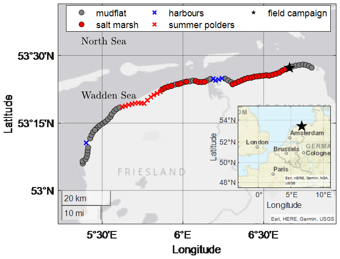
Figure 1 Location of the Dutch Wadden Sea, including its location in Europe (inset). Circles indicate the dikes considered, while “x” symbols were excluded from the analysis. Star indicates the location of the field site at Uithuizerwad.

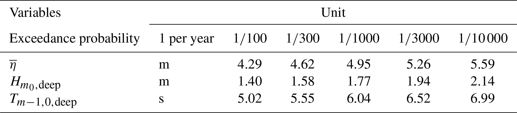
Table 1 Characteristic values for offshore waves and water levels at the Uithuizerwad field site.

The analysis includes the dikes from the city of Harlingen (in the province of Friesland) to those west of Eemshaven (in the province of Groningen), but it excludes the flood defences in front of harbours and areas referred to as summer polders (Fig. 1). Summer polders are low-lying, embanked areas situated in front of the dike and are usually dry in the summer months but may flood during winter storms. As these polders extend for several kilometres, the 1 km transect approach taken here would not be representative.

2.2 Model framework and system description

The model framework used to compute the probability of flooding due to wave overtopping is presented in Fig. 2 and is modified after Vuik et al. (2018b) to include the effect of IG waves. Boundary conditions of offshore wave heights, periods and water levels are transformed over the foreshore to the structure toe using SWAN. These SWAN estimates at the toe are then modified using empirical formulae to account for IG waves. These estimates are then used as input to calculate the actual overtopping discharge, q_a. The probability of failure by wave overtopping, P(Z<0), is then obtained using the first-order reliability method (FORM; Hasofer and Lind, 1974).

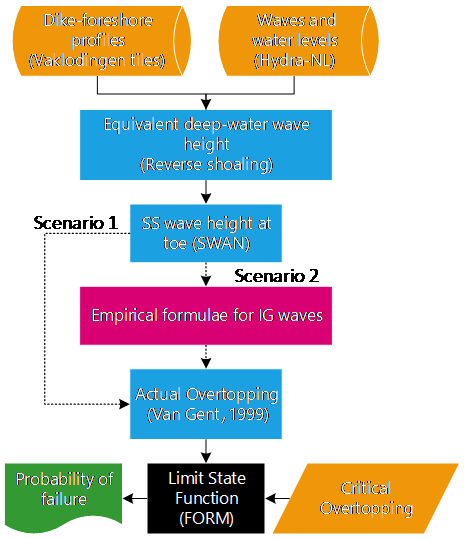
Figure 2 Model framework highlighting Scenario 1, which considers only the influence of SS waves, and Scenario 2, which considers both SS and IG waves (see Sect. 2.2.5 for further scenario descriptions).

While the above framework follows that of Vuik et al. (2018b), there are noteworthy differences between the two approaches. Firstly, the influence of IG waves on both the wave height and the period at the toe is considered – using empirical formulae that are valid for a wide range of foreshore slopes ($\mathrm{10}\le \cot \left(m\right)\le \mathrm{1000}$). Secondly, the effect of wind on wave transformation is neglected here due to close proximity to the shoreline – within 1 km. Lastly, wave attenuation by vegetation is not included in the wider probabilistic analysis because of the following: (i) storms generally occur in the winter season, where there is little vegetation present, and (ii) it is very likely that almost all vegetation present will flatten or break under extreme forcing (Möller et al., 2014; Vuik et al., 2018a). That said, the effect of vegetation (should it be present and remain standing) is demonstrated for one location (Uithuizerwad field site, Fig. 1) in Sect. 3.2 and treated as part of the discussion (Sect. 4.1). The individual components of the model framework are described in detail below. A visual representation of the dike–foreshore system, as well as the various framework components, is provided in Fig. 3.

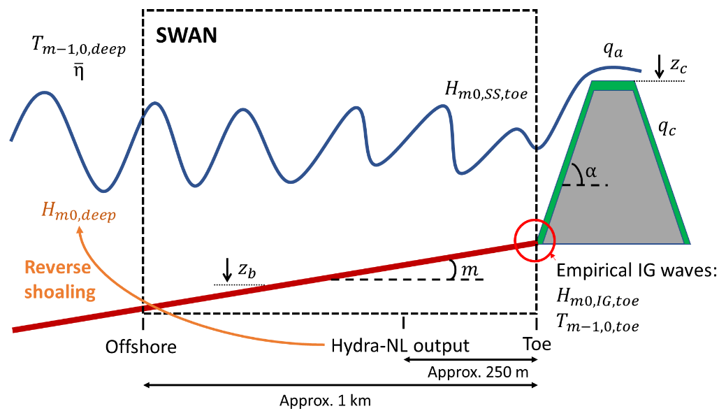
Figure 3 Schematic representation of the dike–foreshore system, showing the areas where key parameters and tools are applied. These parameters include the following: offshore water levels ($\stackrel{\mathrm{‾}}{\mathit{\eta }}$), wave height ($H_{m_{\mathrm{0}},\mathrm{deep}}$), period ($T_{m-\mathrm{1},\mathrm{0},\mathrm{deep}}$), bed level (z_b), foreshore slope (m), dike slope (α), actual overtopping discharge (q_a), crest level (z_c), critical overtopping discharge (q_c), SS-wave height at the toe ($H_{m_{\mathrm{0}},\mathrm{SS},\mathrm{toe}}$), IG-wave height at the toe ($H_{m_{\mathrm{0}},\mathrm{G},\mathrm{toe}}$) and wave period at the toe ($T_{m-\mathrm{1},\mathrm{0},\mathrm{toe}}$).

2.2.1 Boundary conditions

Offshore waves and water levels

To obtain the offshore water levels ($\stackrel{\mathrm{‾}}{\mathit{\eta }}$), wave heights ($H_{m_{\mathrm{0}},\mathrm{deep}}$) and periods ($T_{m-\mathrm{1},\mathrm{0},\mathrm{deep}}$), Hydra-NL (Duits, 2019) – a probabilistic application designed specifically for the assessment and design of flood defences in the Netherlands – was applied. It uses statistics of wind speed, wind direction, water level and their respective correlations to find the corresponding wave characteristics in a pre-calculated database, obtained using the phase-averaged numerical model SWAN (Booij et al., 1999). The tool provides estimates along the entire Dutch Wadden coast, every 250 m, a few hundred metres offshore. To reduce the overall computational time of the probabilistic calculations (around 10 min per dike section), the output locations were reduced to one every 1.5 km (Fig. 1).

The wave heights estimated by Hydra-NL were reverse-shoaled, using linear wave theory, to an offshore point approximately 1 km from the dike toe (Fig. 3). This was done to obtain estimates of the offshore wave height ($H_{m_{\mathrm{0}},\mathrm{deep}}$) for use with Eq. (12). Compared to the Hydra-NL estimates (a few hundred metres offshore), the reverse-shoaled significant wave heights (1 km offshore) were on average 2 % higher, with a maximum increase of 4 % and maximum reduction of 9 %. In this approach, the effects of friction and refraction are neglected. Likewise it is assumed that no local generation or wave breaking occurred. The assumption of non-breaking waves is considered reasonable, since the average ratio of the wave height to water depth at the Hydra-NL output location was 0.37, while the average ratio for breaking waves – referred to as the breaker index – was estimated as 0.79 (using Eq. 4). In addition, due to the close proximity to the shoreline (within 1 km), it is unlikely that local generation by wind would be significant.

For each location, five exceedance probabilities were considered in Hydra-NL: $\mathrm{1}/\mathrm{100}$, $\mathrm{1}/\mathrm{300}$, $\mathrm{1}/\mathrm{1000}$, $\mathrm{1}/\mathrm{3000}$ and $\mathrm{1}/\mathrm{10}\mathrm{000}$ per year (Table 1). Using the $\stackrel{\mathrm{‾}}{\mathit{\eta }}$, $H_{m_{\mathrm{0}},\mathrm{deep}}$ and $T_{m-\mathrm{1},\mathrm{0},\mathrm{deep}}$ estimates for each probability of exceedance, Weibull distribution parameters – namely, scale and shape parameters – were derived to accurately describe the extremes. The range of the scale and shape parameter values is provided in Table A1.

Dike–foreshore characteristics

The bathymetry of the Dutch coast, from dry land up to the 20 m isobath in the North Sea, is continuously measured (at least once every 7 years) by the Dutch government (Rijkswaterstaat). This dataset, referred to as “Vaklodingen” (Wiegmann et al., 2005), covers the Wadden Sea with a 20 m grid resolution (Fig. 4). Cross-shore transects of approximately 1 km, at alongshore intervals corresponding to the Hydra-NL output locations, were extracted considering a NW–SE orientation – in-line with the dominant wind–wave direction during storms (NW) (Vuik et al., 2018b). By aligning the transect with the dominant wind–wave direction, the influence of wave obliqueness on wave overtopping, which is typically taken into account using a correction factor, may be neglected (Willemsen et al., 2020). It should be noted that assuming a NW–SE orientation results in an artificially milder dike slope for dikes that are not perpendicular to the assumed transect. This is taken into account in the average dike slope calculation.

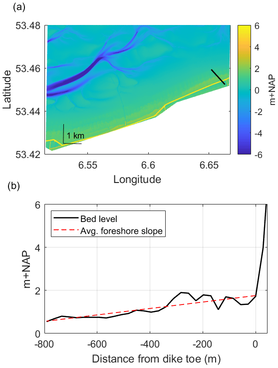
Figure 4 Subset of the Vaklodingen bathymetry dataset showing (a) a NW–SE-oriented transect at the field site location, Uithuizerwad (black line), and (b) the corresponding cross-shore profile of this transect with the estimated average foreshore slope.

For each transect, the mean elevation  (z_b) and average foreshore slopes (tan (m)) were obtained. To account for variations in bathymetry and measurement inaccuracies, z_b was treated as a normally distributed parameter with a standard deviation of 0.2 m (Vuik et al., 2018b). The average slope was determined as the best-fit line (least-squares method) considering the foreshore elevation data points between the dike toe and 1 km offshore. While the actual bathymetry is used for the numerical modelling of the SS waves, the estimated tan (m) is necessary for use with the empirical formulae for the influence of the IG waves (Sect. 2.2.2). Given the range of validity of the empirical formulae (Eqs. 12 and 18), a minimum foreshore slope of $\mathrm{1}/\mathrm{1000}$ (or 0.1 %) is considered here. This is in line with the common approach where slopes milder than or equal to 0.1 % are treated equally as (nearly) flat (Keimer et al., 2021; Steendam et al., 2004). Note that the calculated foreshore slopes ranged from −0.04 % to 4 % with an average of 0.14 %, where a negative slope indicates a slight downward slope towards the dike toe.

Given the significant influence of the dike geometry on the calculated probability of failure (Sect. 3.2.2), the crest level (z_c) and average dike slope (tan (α)) were treated here as deterministic parameters with the same values applied to each location. This was done to remove the influence of variations in dike geometry on the calculated failure probabilities and allow the analysis to focus on what occurs over the foreshore. The crest levels were set to 6 m + NAP, corresponding to the required safety level (probability of failure less than $\mathrm{1}/\mathrm{1000}$ per year). Similarly, the dike slopes were set to $\mathrm{1}/\mathrm{7}$ to represent the average slope of a typical Wadden Sea dike, which is often characterized by 1:4 upper and lower slopes separated by a mildly sloping berm. This value also accounts for the NW–SE orientation, which results in an artificially milder average dike profile. Note that an analysis of the sensitivity of the estimated probability of failure to variations in z_c, including its treatment as deterministic versus stochastic, is provided in Sect. 3.2.2. It should be noted that the actual crest levels of the Dutch Wadden Sea dikes typically exceed 8 m + NAP; however, a crest level this high would result in extremely small failure probabilities, which would distract from the findings herein.

2.2.2 Wave transformation

Numerical model for SS waves: SWAN

SWAN is a third-generation, phase-averaged wave model used to estimate the generation (by wind), propagation and dissipation (by depth-induced breaking and bottom friction) of waves from offshore to the structure toe (Booij et al., 1999). This includes wave–wave interactions, in both deep and shallow water, and wave-induced setup but neglects wave-induced currents and the generation or propagation of IG waves. SWAN computes the spectral evolution of wave action density (A) in space and time. For stationary 1D simulations, the governing equations follow

$$\begin{array}{}\text{(1)}& {\displaystyle \frac{\partial c_{x}A}{\partial x}}={\displaystyle \frac{S_{\mathrm{tot}}}{\mathit{\omega }}},\end{array}$$

where c_x is the propagation velocity of wave energy in the x direction; ω is the frequency; and S_tot may include dissipation terms due to depth-limited wave breaking (${\stackrel{\mathrm{‾}}{D}}_{\mathrm{w}}$), vegetation (${\stackrel{\mathrm{‾}}{D}}_{\mathrm{v}}$) and bottom friction, and energy transfer terms.

To simulate depth-limited wave breaking, SWAN uses the following parametric dissipation model, by default (Battjes and Janssen, 1978)

$$\begin{array}{}\text{(2)}& {\stackrel{\mathrm{‾}}{D}}_{\mathrm{w}}={\displaystyle \frac{\mathit{\alpha }}{\mathrm{4}}}\mathit{\rho }g{f}_{\mathrm{mean}}{Q}_{\mathrm{b}}{H}_{\max }^{\mathrm{2}},\end{array}$$

and Q_b is estimated as

$$\begin{array}{}\text{(3)}& {\displaystyle \frac{\mathrm{1}-Q_{\mathrm{b}}}{\ln Q_{\mathrm{b}}}}=-\mathrm{8}{\displaystyle \frac{E_{\mathrm{tot}}}{H_{\max }^{\mathrm{2}}}},\end{array}$$

where f_mean is the mean wave frequency, H_max=γ_bjh and E_tot is the total wave energy variance. Here, the breaker parameter (γ_bj) is based on the offshore wave steepness, $s_{\mathrm{0}}=H_{\mathrm{rms}}/L_{\mathrm{0}}$ (Battjes and Stive, 1985), as

$$\begin{array}{}\text{(4)}& {\mathit{\gamma }}_{\mathrm{b}j}=\mathrm{0.5}+\mathrm{0.4}\tanh \left(\mathrm{33}\cdot s_{\mathrm{0}}\right),\end{array}$$

where H_rms is the root mean square wave height, with $H_{\mathrm{rms}}=\sqrt{\mathrm{8}\cdot E_{\mathrm{tot}}}$. Following Vuik et al. (2018b), γ_bj is treated as a normally distributed parameter with a standard deviation of 0.05 and mean value determined using Eq. (4).

As recommended by Baron-Hyppolite et al. (2018), the explicit vegetation representation in SWAN – which was implemented by Suzuki et al. (2012) – is applied. This method represents vegetation as rigid cylinders, following the approach of Dalrymple et al. (1984) modified for irregular waves by Mendez and Losada (2004). In this approach, the mean rate of energy dissipation per unit horizontal area due to wave damping by vegetation (ϵ_v) is given by the following:

$$\begin{array}{}\text{(5)}& \begin{array}{rl}{\stackrel{\mathrm{‾}}{D}}_{\mathrm{v}}=& {\displaystyle \frac{\mathrm{1}}{\mathrm{2}g\sqrt{\mathit{\pi }}}}\mathit{\rho }{C}_{\mathrm{D}}{b}_{\mathrm{v}}{N}_{\mathrm{v}}{\left({\displaystyle \frac{gk}{\mathrm{2}{f}_{\mathrm{mean}}}}\right)}^{\mathrm{3}}\\ & {\displaystyle \frac{{\sinh }^{\mathrm{3}}k{h}_{\mathrm{v}}+\mathrm{3}\sinh k{h}_{\mathrm{v}}}{\mathrm{3}k\cos h^{\mathrm{3}}kh}}{H}_{\mathrm{rms}}^{\mathrm{3}},\end{array}\end{array}$$

where ρ is the density of water, g is the gravitational acceleration, k is the mean wave number, h is the water depth, C_D (0.4) is the drag coefficient, b_v (3 mm) is the stem diameter, N_v (1200 stems m⁻²) is the vegetation density and h_v (0.3 m) is the vegetation height; the values in parentheses are representative of salt marshes in the Netherlands (Vuik et al., 2016).

Deep-water processes such as white capping, wind and quadruplet wave–wave interactions were disabled, while triad wave–wave interactions, a shallow water process, were activated. All other model parameters were kept at their default values. For all simulations, a constant grid spacing of 2.5 m was applied. This corresponded to approximately 15–20 grid cells per deep-water wavelength.

Empirical formulae for the influence of IG waves

The influence of the IG waves may be represented by an increase in the design parameters, namely the total significant wave height ($H_{m_{\mathrm{0}},\mathrm{toe}}$) and spectral wave period ($T_{m-\mathrm{1},\mathrm{0},\mathrm{toe}}$) at the toe based on incident waves, where

$$\begin{array}{}\text{(6)}& {\displaystyle }& {\displaystyle }{H}_{m_{\mathrm{0}}}=\sqrt{H_{m_{\mathrm{0}},\mathrm{SS}}^{\mathrm{2}}+H_{m_{\mathrm{0}},\mathrm{IG}}^{\mathrm{2}}};\text{(7)}& {\displaystyle }& {\displaystyle }{H}_{m_{\mathrm{0}},\mathrm{SS}}=\mathrm{4}\sqrt{\underset{\mathrm{0.05}}{\overset{\mathrm{1}}{\int }}{C}_{\mathit{\eta }\mathit{\eta }}df};\text{(8)}& {\displaystyle }& {\displaystyle }{H}_{m_{\mathrm{0}},\mathrm{IG}}=\mathrm{4}\sqrt{\underset{\mathrm{0.005}}{\overset{\mathrm{0.05}}{\int }}{C}_{\mathit{\eta }\mathit{\eta }}df};\end{array}$$

and

$$\begin{array}{}\text{(9)}& T_{m-\mathrm{1},\mathrm{0}}={\displaystyle \frac{m_{-\mathrm{1}}}{m_{\mathrm{0}}}},\end{array}$$

where

$$\begin{array}{}\text{(10)}& m_n=\sqrt{\underset{\mathrm{0.005}}{\overset{\mathrm{1}}{\int }}{C}_{\mathit{\eta }\mathit{\eta }}\cdot f^{n}df},\end{array}$$

where C_ηη(f) is the wave energy density and 0.05 Hz is the frequency separating SS and IG motions. It should be noted that for conditions with a single, clearly defined peak frequency (f_p), the frequency separating IG and SS motions is typically taken as $f_{\mathrm{p}}/\mathrm{2}$. However, as wave spectra in the Dutch Wadden Sea typically show multiple peaks, a separation frequency of 0.05 Hz is typically used to avoid contaminating the IG signal with that of swell (with periods around 10 s or 0.1 Hz). This choice of split frequency is consistent with previous studies in the area (Engelstad et al., 2017; De Bakker et al., 2014) and coincides with the minimum in spectral density observed in the field data (Fig. B1).

Influence on significant wave height at the toe

The relative magnitude or significance of IG waves at the toe of the dike (${\stackrel{\mathrm{̃}}{H}}_{\mathrm{IG}}$) may be expressed as the following:

$$\begin{array}{}\text{(11)}& {\stackrel{\mathrm{̃}}{H}}_{\mathrm{IG}}={\displaystyle \frac{H_{m_{\mathrm{0}},\mathrm{IG},\mathrm{toe}}}{H_{m_{\mathrm{0}},\mathrm{SS},\mathrm{toe}}}}.\end{array}$$

Using a numerical dataset of 672 XBeach non-hydrostatic (Smit et al., 2010) simulations with varied $H_{m_{\mathrm{0}},\mathrm{deep}}$, $T_{m-\mathrm{1},\mathrm{0},\mathrm{deep}}$, h_toe, m, α, wave directional spreading (σ_dir) and width of vegetated cover (W_veg) parameter values, Lashley et al. (2020a) derived the following formulae to estimate ${\stackrel{\mathrm{̃}}{H}}_{\mathrm{IG}}$:

$$\begin{array}{}\text{(12)}& {\stackrel{\mathrm{̃}}{H}}_{\mathrm{IG}}=C\cdot H_{m_{\mathrm{0}},\mathrm{deep}}^{\mathrm{0.5}}\cdot {\stackrel{\mathrm{‾}}{\mathit{\gamma }}}_{\mathit{\sigma }}\cdot {\stackrel{\mathrm{‾}}{\mathit{\gamma }}}_{\mathrm{h}}\cdot {\stackrel{\mathrm{‾}}{\mathit{\gamma }}}_{\mathrm{f}}\cdot {\stackrel{\mathrm{‾}}{\mathit{\gamma }}}_{\mathrm{v}}\cdot {\stackrel{\mathrm{‾}}{\mathit{\gamma }}}_{\mathrm{d}},\end{array}$$

where the coefficient (C) is 0.36 m^−0.5 and ${\stackrel{\mathrm{‾}}{\mathit{\gamma }}}_{\mathit{\sigma }}$, ${\stackrel{\mathrm{‾}}{\mathit{\gamma }}}_{\mathrm{h}}$, ${\stackrel{\mathrm{‾}}{\mathit{\gamma }}}_{\mathrm{f}}$, ${\stackrel{\mathrm{‾}}{\mathit{\gamma }}}_{\mathrm{v}}$ and ${\stackrel{\mathrm{‾}}{\mathit{\gamma }}}_{\mathrm{d}}$ are influence factors for wave directional spreading, water depth at the toe, foreshore slope, vegetated cover and structure slope, respectively. For the probabilistic analysis, Eq. (12) is multiplied by a normally distributed factor (f_IG) with a mean (0.99) and standard deviation (0.18) based on the bias and scatter observed during its derivation, respectively (Lashley et al., 2020a).

The individual factors are detailed below:

$$\begin{array}{}\text{(13)}& {\stackrel{\mathrm{‾}}{\mathit{\gamma }}}_{\mathit{\sigma }}=\mathrm{1}-\mathrm{0.01}\cdot {\mathit{\sigma }}_{\mathrm{dir}},\end{array}$$

where the wave directional spreading, σ_dir=24^∘ to represent the wind-sea conditions of the Wadden Sea.

$$\begin{array}{}\text{(14)}& {\displaystyle }{\stackrel{\mathrm{‾}}{\mathit{\gamma }}}_{\mathrm{h}}=\mathrm{1.04}\cdot \exp \left(-\mathrm{1.4}\cdot h_{\mathrm{toe}}\right)+\mathrm{0.9}\cdot \exp \left(-\mathrm{0.19}\cdot h_{\mathrm{toe}}\right),\text{(15)}& {\displaystyle }\begin{array}{rl}& {\stackrel{\mathrm{‾}}{\mathit{\gamma }}}_{\mathrm{f}}=\\ & \left\{\begin{array}{ll}\mathrm{1.56}-\mathrm{3.09}\cdot \cot (m{)}^{-\mathrm{0.44}}& \cot \left(m\right)\le \mathrm{100}\\ \mathrm{0.51}\cdot \cot (m{)}^{\mathrm{0.18}}& \cot \left(m\right)>\mathrm{100},h_{\mathrm{toe}}/H_{m_{\mathrm{0}},\mathrm{deep}}\ge \mathrm{0.2}\\ \mathrm{1.62}\cdot \cot (m{)}^{-\mathrm{0.08}}& \cot \left(m\right)>\mathrm{100},h_{\mathrm{toe}}/H_{m_{\mathrm{0}},\mathrm{deep}}<\mathrm{0.2}\end{array}\right.,\end{array}\text{(16)}& {\displaystyle }{\stackrel{\mathrm{‾}}{\mathit{\gamma }}}_{\mathrm{v}}=\mathrm{0.94}\cdot e^{-W_{\mathrm{veg}}/\mathrm{500}}+\mathrm{0.06}\cdot e^{W_{\mathrm{veg}}/\mathrm{500}},\end{array}$$

where W_veg is measured as the horizontal, cross-shore width of the vegetated cover. It should be noted that the influence of vegetation on IG waves was assessed for very shallow conditions ($h_{\mathrm{toe}}/h_{\mathrm{v}}=\mathrm{3.3}$); therefore, the performance of Eq. (16) for vegetation with larger ratios of water depth to stem height is yet to be verified. Lastly, to account for the influence of waves reflected at the dike slope,

$$\begin{array}{}\text{(17)}& {\stackrel{\mathrm{‾}}{\mathit{\gamma }}}_{\mathrm{d}}=\mathrm{1.3}-\mathrm{0.02}\cdot \cot (\mathit{\alpha }{)}^{\mathrm{2}}+\mathrm{0.24}\cdot \cot (\mathit{\alpha }).\end{array}$$

For an analysis of incident waves only, ${\stackrel{\mathrm{‾}}{\mathit{\gamma }}}_{\mathrm{d}}=\mathrm{1}$.

The above approach (Eq. 12) accounts for IG-wave generation by the following: (i) bound-wave shoaling over mildly sloping bathymetry and (ii) the temporal variation in the location of breaking waves, known as the break-point forcing mechanism (Battjes, 2004). However, it does not account for IG waves that may be refractively trapped, known as edge waves, or those reflected from a distant coast, known as leaky waves (Elgar et al., 1992; Bertin et al., 2018; Reniers et al., 2021). The relevance of these free IG waves to the Dutch Wadden Sea coast is still to be confirmed.

Influence on the spectral wave period at the toe

The existing method to estimate the increase in the spectral wave period at the toe due to IG waves in shallow water, developed by Hofland et al. (2017), was based on laboratory tests with foreshore slopes, $\mathrm{35}<\cot \left(m\right)<\mathrm{250}$. While the method proved accurate within this range, it tended to underestimate $T_{m-\mathrm{1},\mathrm{0},\mathrm{toe}}$ for slopes gentler than 1:250 (Nguyen et al., 2020). As foreshores in the Wadden Sea are typically 1:500 to (nearly) flat, a new formulation for $T_{m-\mathrm{1},\mathrm{0},\mathrm{toe}}$ is derived here – using the above-mentioned numerical dataset (Lashley et al., 2020a).

Since $T_{m-\mathrm{1},\mathrm{0},\mathrm{toe}}$ and ${\stackrel{\mathrm{̃}}{H}}_{\mathrm{IG}}$ both describe the amount of energy in the IG band compared to the SS band, it stands to reason that a simple relation should exist between the two parameters. From the Lashley et al. (2020a) numerical dataset with $\mathrm{10}<\cot \left(m\right)<\mathrm{1000}$, the following relationship between $T_{m-\mathrm{1},\mathrm{0},\mathrm{toe}}/T_{m-\mathrm{1},\mathrm{0},\mathrm{deep}}$, ${\stackrel{\mathrm{̃}}{H}}_{\mathrm{IG}}$ and cot α_fore was found (R²=0.92):

$$\begin{array}{}\text{(18)}& {\displaystyle \frac{T_{m-\mathrm{1},\mathrm{0},\mathrm{toe}}}{T_{m-\mathrm{1},\mathrm{0},\mathrm{deep}}}}=\left\{\begin{array}{ll}\mathrm{1.59}\cdot {\stackrel{\mathrm{̃}}{H}}_{\mathrm{IG}}^{\mathrm{0.69}}\cdot \cot (m{)}^{\mathrm{0.17}}& \frac{h_{\mathrm{toe}}}{H_{m_{\mathrm{0}},\mathrm{deep}}}\le \mathrm{1}\\ \mathrm{1}& \frac{h_{\mathrm{toe}}}{H_{m_{\mathrm{0}},\mathrm{deep}}}>\mathrm{1}\end{array}\right..\end{array}$$

Further details on the derivation of Eq. (18) and its performance in comparison to the Hofland et al. (2017) model are provided in Appendix C. For the probabilistic analysis, Eq. (18) is multiplied by a normally distributed factor ($f_{T_m}$) with a mean (0.99) and standard deviation (0.17) based on the bias and scatter observed during its derivation, respectively.

2.2.3 Wave overtopping

Empirical formulae for actual wave overtopping

In the present study, the overtopping formula proposed by Van Gent (1999) (Eq. 19) is applied. This formula was chosen because it (i) was developed specifically for shallow foreshores, (ii) considers the influence of both SS and IG waves, and (iii) is considered valid for a wide range of breaker parameter (${\mathit{\xi }}_{m-\mathrm{1},\mathrm{0}}$) values.

$$\begin{array}{}\text{(19)}& {\displaystyle \frac{q_{\mathrm{a}}}{\sqrt{g\cdot H_{m_{\mathrm{0}},\mathrm{toe}}^{\mathrm{3}}}}}={\mathrm{10}}^{\mathrm{c}}\cdot \exp \left(-{\displaystyle \frac{R_{\mathrm{c}}}{H_{m_{\mathrm{0}},\mathrm{toe}}\cdot \left(\mathrm{0.33}+\mathrm{0.022}\cdot {\mathit{\xi }}_{m-\mathrm{1},\mathrm{0}}\right)}}\right),\end{array}$$

where

$$\begin{array}{}\text{(20)}& {\displaystyle }& {\displaystyle }{\mathit{\xi }}_{m-\mathrm{1},\mathrm{0}}={\displaystyle \frac{\tan \left(\mathit{\alpha }\right)}{\sqrt{H_{m_{\mathrm{0}},\mathrm{toe}}/L_{m-\mathrm{1},\mathrm{0}}}}},\text{(21)}& {\displaystyle }& {\displaystyle }{L}_{m-\mathrm{1},\mathrm{0}}={\displaystyle \frac{g\cdot T_{m-\mathrm{1},\mathrm{0},\mathrm{toe}}^{\mathrm{2}}}{\mathrm{2}\mathit{\pi }}},\end{array}$$

where g is the gravitational constant of acceleration, α is the dike slope, ${\mathit{\xi }}_{m-\mathrm{1},\mathrm{0}}$ is the Iribarren number (also referred to as the breaker parameter) and $L_{m-\mathrm{1},\mathrm{0}}$ is a fictitious wavelength based on the spectral wave period at the toe. It is important to note that $H_{m_{\mathrm{0}},\mathrm{toe}}$ and $T_{m-\mathrm{1},\mathrm{0},\mathrm{toe}}$ in the above equations are based on the incident waves (i.e. without the influence of wave reflection at the structure). The empirical coefficient (c) is a normally distributed parameter with a mean of −0.92 and a standard deviation of 0.24. Here, Eq. (19) is applied to all locations, regardless of the ${\mathit{\xi }}_{m-\mathrm{1},\mathrm{0}}$ value. However, it should be noted that this approach does not coincide with the current standard (EurOtop, 2018). EurOtop (2018) recommends that different formulae be applied depending on the ${\mathit{\xi }}_{m-\mathrm{1},\mathrm{0}}$ value (Van der Meer and Bruce, 2014; Altomare et al., 2016). However, due to the gentle dike (1:7) and foreshore slopes (1:600, on average) considered here, applying the EurOtop (2018) approach proved challenging. This is discussed in detail in Sect. 4.2.

The dikes of the Dutch Wadden Sea are typically grass-covered and therefore treated as smooth (without roughness elements). To simplify the calculation, the dikes are assumed to be uniformly sloping (without a berm). However, it should be noted that the presence of berms and roughness elements could significantly reduce the overtopping discharge (Bruce et al., 2009; Chen et al., 2020; Van der Meer, 2002).

Critical wave overtopping

The erosion resistance of the grass-covered landward slope of the dike is described by a critical or tolerable overtopping discharge (q_c). Given the significant influence of this parameter on the probability of dike failure by wave overtopping (Sect. 3.2.2), it is treated here as a deterministic parameter with a value of 50 L s⁻¹ m⁻¹ for each location. In this way, the influence of other parameters, such as those linked to the IG waves, can be better assessed. An analysis of the sensitivity of the estimated probability of failure to changes in q_c is provided in Sect. 3.2.2. This analysis also demonstrates how the probability of failure would change if q_c were instead treated as a stochastic parameter.

2.2.4 Probabilistic methods

FORM

The open-source implementation of FORM, part of OpenEarthTools (Van Koningsveld et al., 2010), is used to evaluate the limit state function (LSF) for any possible combination of input variables, which are each described by probability distributions. The following LSF is considered here (Oosterlo et al., 2018):

$$\begin{array}{}\text{(22)}& Z=\log q_{\mathrm{c}}-\log q_{\mathrm{a}},\end{array}$$

where Z is the limit state considering the critical (q_c) and actual (q_a) overtopping discharges, which represent the resistance and load, respectively, and the probability of failure by wave overtopping, $P_{\mathrm{f}}=P(Z<\mathrm{0})$ or P(q_a>q_c).

FORM simplifies the mathematical problem by linearizing the LSF and transforming all probability distributions to equivalent normal distributions. P_f is then expressed in terms of a reliability index (β), which represents the minimum distance from the most probable failure point on the limit state surface (Z=0), referred to as the design point, to the origin of the transformed coordinate system (Hasofer and Lind, 1974).

$$\begin{array}{}\text{(23)}& \mathit{\beta }={\displaystyle \frac{{\mathit{\mu }}_z}{{\mathit{\sigma }}_z}},\end{array}$$

where μ_z and σ_z are the mean and standard deviation of the limit-state function (Z), respectively, and

$$\begin{array}{}\text{(24)}& P_{\mathrm{f}}=\mathrm{\Phi }(-\mathit{\beta }),\end{array}$$

where Φ is the cumulative distribution function for a standard normal variable.

FORM starts in a user-defined position in the probability density functions of all variables (e.g. the mean value). It then uses an iterative procedure to update the design point until convergence is achieved (Vuik et al., 2018b). In each iteration, FORM tests how strong the LSF responds to a perturbation of each individual variable, X_i. The response is expressed in terms of the partial derivative $\partial Z/\partial X_{\mathrm{i}}$, which is then used to calculate sensitivity factors (α_sf,i):

$$\begin{array}{}\text{(25)}& {\mathit{\alpha }}_{\mathrm{sf},\mathrm{i}}={\displaystyle \frac{\partial Z/\partial X_i\cdot {\mathit{\sigma }}_i}{{\mathit{\sigma }}_z}},\end{array}$$

where α_sf,i represents the relative importance of the uncertainty in each stochastic parameter such that $\sqrt{\sum _{i=\mathrm{1}}^n{\mathit{\alpha }}_{\mathrm{sf},\mathrm{i}}^{\mathrm{2}}}=\mathrm{1}$. Uncertainties in parameters with large α_sf values – that is, values closer to 1 – are considered to be significant such that a small change in the uncertainty of that parameter would result in a relatively large change in the reliability index (β). However, the uncertainty in parameters with α_sf values close to 0 have minor relative importance, and those parameters may be treated as deterministic (Kjerengtroen and Comer, 1996). An analysis of the sensitivity factors determined for the filed site location at Uithuizerwad is presented in Appendix D.

Dependencies

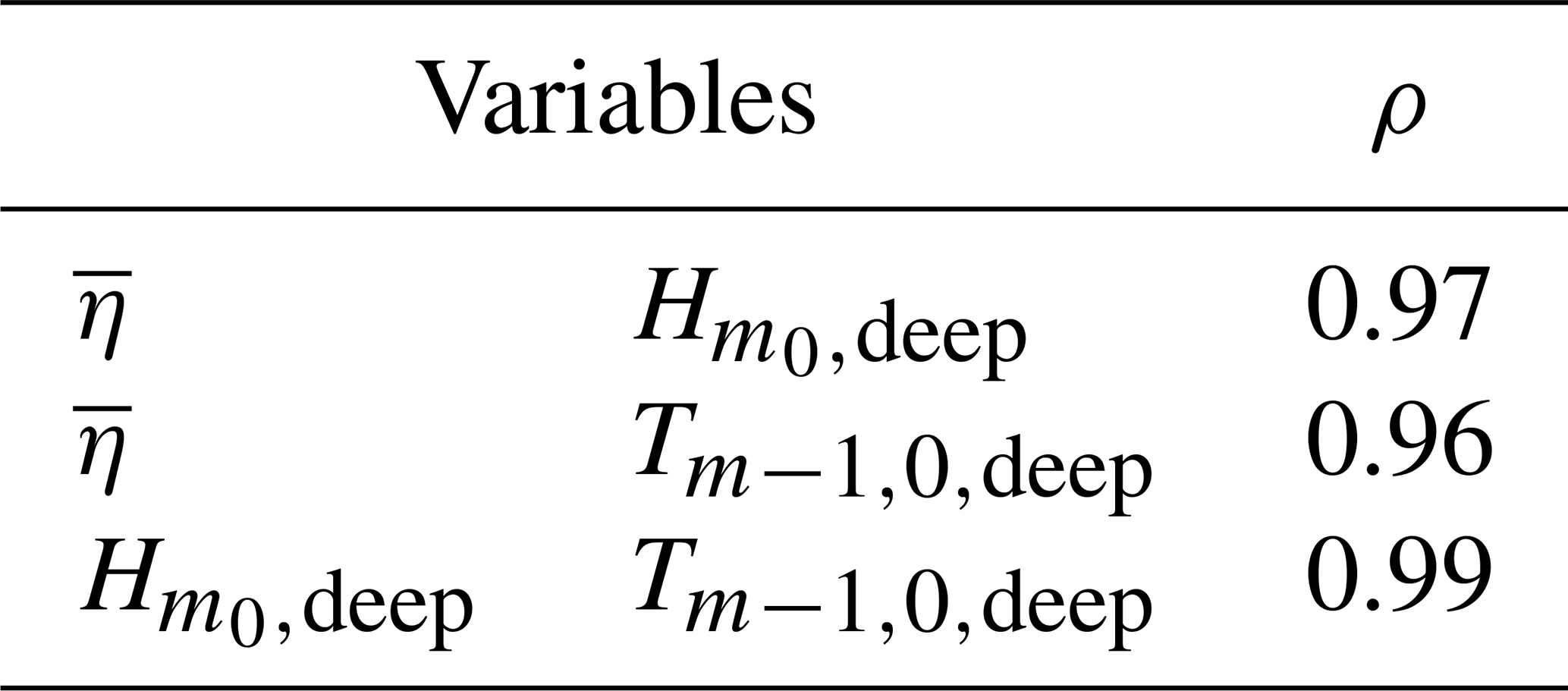
The following (Gaussian) dependencies between variables are imposed (Table 2); all other variables are considered independent.

Table 2 Pearson correlation coefficients (ρ) for Gaussian dependence between boundary conditions ($\stackrel{\mathrm{‾}}{\mathit{\eta }}$, $H_{m_{\mathrm{0}},\mathrm{deep}}$ and $T_{m-\mathrm{1},\mathrm{0},\mathrm{deep}}$). Source: Vuik et al. (2018b).

2.2.5 Foreshore scenarios

In order to investigate the effect of IG waves on the P_f value, we consider the following two scenarios (Fig. 2):

1. SS-wave breaking, where the influence of the foreshore bathymetry on incident SS waves is considered but IG waves are neglected, and

2. SS-wave breaking and IG waves, where the influence of the foreshore bathymetry on both SS and IG waves are considered.

Note that the influence of bottom roughness on wave propagation is included in both scenarios and represented by default parameter values in the numerical model. In the Netherlands, Scenario 1 represents standard practice, as the influence of IG waves are typically not considered during safety assessments. By assessing the difference in P_f between Scenario 1 and Scenario 2 – hereafter, referred to as $P_{{\mathrm{f}}_{\mathrm{1}}}$ and $P_{{\mathrm{f}}_{\mathrm{2}}}$, respectively – the influence of the IG waves may be quantified. Note that in both scenarios vegetation is assumed to be flattened, broken or not present (mudflats) in the analysis of the wider Wadden Sea coast. However, the influence of standing vegetation on the P_f value is demonstrated for a single case at the Uithuizerwad location in Sect. 3.2.

2.3 Field data for model validation

The performance of the combined numerical and empirical wave modelling approach is assessed by comparing estimates to storm data measured at Uithuizerwad, the Dutch Wadden Sea (Fig. 1) – where the dike is fronted by vegetated foreshore with an average foreshore slope of 1:600. In this way, the ability of the approach to accurately represent the processes occurring over the foreshore is verified as namely (i) the decrease in SS waves due to depth-induced breaking over the foreshore and (ii) the increase in wave height and period at the toe due to IG waves. This dataset is described below.

Two field campaigns were carried out in winter 2014/15 and 2016/17 at Uithuizerwad (Fig. 1), capturing severe storms on 11 January 2015 and 13 January 2017, both with exceedance probabilities of approximately $\mathrm{1}/\mathrm{5}$ per year (Zhu et al., 2020). Here, we consider two transects of wave gauges that captured the change in wave conditions from the marsh edge to dike toe (Fig. 5). In January 2015, a transect of five pressure gauges (Ocean Sensor Systems, Inc., USA) was deployed nearshore, each sampling at 5 Hz over a period of 7 min, every 15 min (Fig. 5a). In January 2017, the setup of the experiment was slightly altered with four gauges deployed, each sampling continuously at 5 Hz (Fig. 5b).

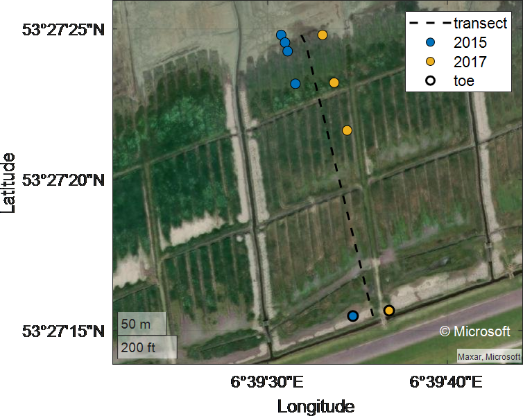
Figure 5 Wave gauges locations for the January 2015 and January 2017 field campaigns at Uithuizerwad (see star in Fig. 1).

The pressure signal from each gauge was translated into time series of surface elevations, using linear wave theory to adjust for attenuation of the pressure signal with depth. After that, a Fourier transform was performed to transform the data from the time domain to the frequency domain (Hann window, 50 % overlap). To improve the frequency resolution of the resulting wave spectra, measurements from two successive bursts were combined into a single time record. For the 2015 dataset, this yielded spectra with 19 degrees of freedom and a frequency resolution of 0.011 Hz, while the analysis of the 2017 dataset yielded spectra with 31 degrees of freedom and a frequency resolution of 0.0089 Hz (Appendix B). The measured wave and water level conditions at the marsh edge for the 2015 and 2017 winter storms are summarized in Table 3.

Table 3 Measured waves and water levels at the marsh edge during the 2015 and 2017 winter storms at Uithuizerwad.

3 Results

3.1 Validation of wave modelling

In this section, the comparison between the combined numerical and empirical modelling approach for wave transformation (Sect. 2.2.2) and the field measurements (Sect. 2.3) is presented. For both the 2015 and 2017 storms, SWAN is set up as a transect (1D) in line with wave sensors (Fig. 5). In each simulation, the numerical model is forced at its boundary with the measured wave spectra at the most offshore wave sensor. SWAN is able to capture the dissipation of SS waves due to the combined effects of the shallow bathymetry and vegetation (Fig. 6). In 2015, the modelled SS-wave attenuation from the most offshore gauge to the dike toe was 56 %, half of which (28 %) was due to depth-induced wave breaking over the shallow bathymetry alone. Similarly, modelled SS-wave attenuation in 2017 was 63 % with 39 % due to depth-induced wave breaking alone.

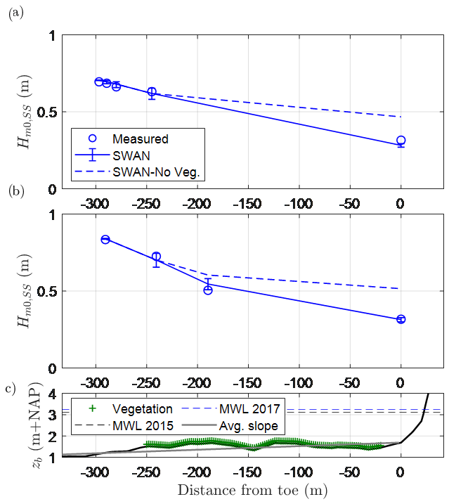
Figure 6 Comparison of measured and modelled significant wave heights in the SS bands ($H_{m_{\mathrm{0}},\mathrm{SS}}$) at the peaks of the (a) January 2015 and (b) January 2017 storms at Uithuizerwad (see Fig. 5 for gauge locations). Error bars represent the uncertainty in the estimates based on the standard deviation of Eq. (4). Panel (c) shows the bed level and vegetated cover. MWL: mean water level (at the peak of the storm).

At the toe of the dike, Eqs. (12) and (18) are used to estimate the increase in the relative magnitude of the IG waves, ${\stackrel{\mathrm{̃}}{H}}_{\mathrm{IG}}$ (Fig. 7), and the associated increase in the spectral wave period relative to its deep-water value, $T_{m-\mathrm{1},\mathrm{0},\mathrm{toe}}/T_{m-\mathrm{1},\mathrm{0},\mathrm{deep}}$ (Fig. 8), respectively. Compared to the measurements at the toe (Eq. 11), Eq. (12) produced an average error of −5 %; that is, predictions were, on average, 5 % lower than the measurements. In Fig. 8, estimates of $T_{m-\mathrm{1},\mathrm{0},\mathrm{toe}}/T_{m-\mathrm{1},\mathrm{0},\mathrm{deep}}$ made by SWAN and the Hofland et al. (2017) formula are also presented for comparison. For the two storms, SWAN produced an average error of −48 % compared to Eq. (18) with 11 % error, thus indicating the relevance of IG waves. Similarly, the Hofland et al. (2017) formula produced an average error of −55 %. As the Hofland et al. (2017) formula is based on tests with $\mathrm{35}\le \cot \left(m\right)\le \mathrm{250}$, these results further indicate that it should not be applied outside of this range and highlights the added value of Eq. (18) – which considers slopes as gentle as 1:1000.

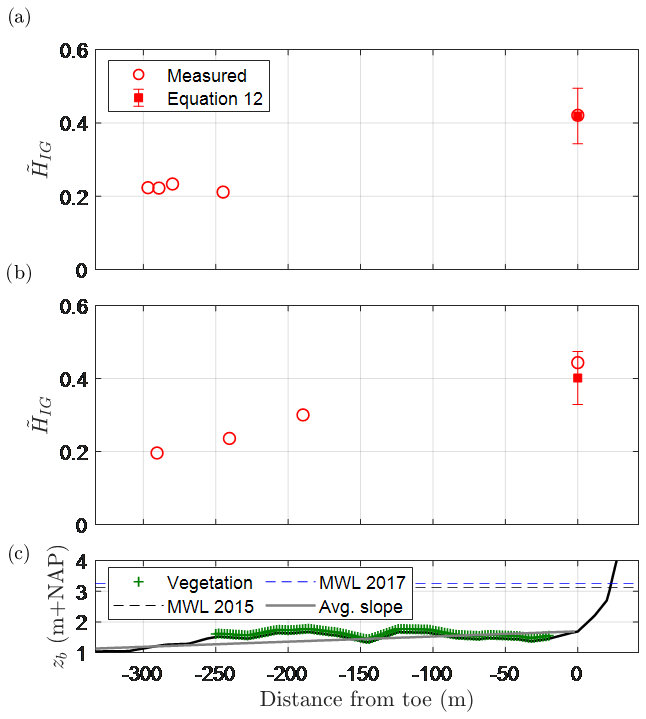
Figure 7 Comparison of measured and modelled relative magnitude of the IG waves (${\stackrel{\mathrm{̃}}{H}}_{\mathrm{IG}}$) at the peaks of the (a) January 2015 and (b) January 2017 storms at Uithuizerwad (see Fig. 5 for gauge locations). Error bars represent the uncertainty in the estimates based on the standard deviation of Eq. (12). Panel (c) shows the bed level and vegetated cover. MWL: mean water level (at the peak of the storm).

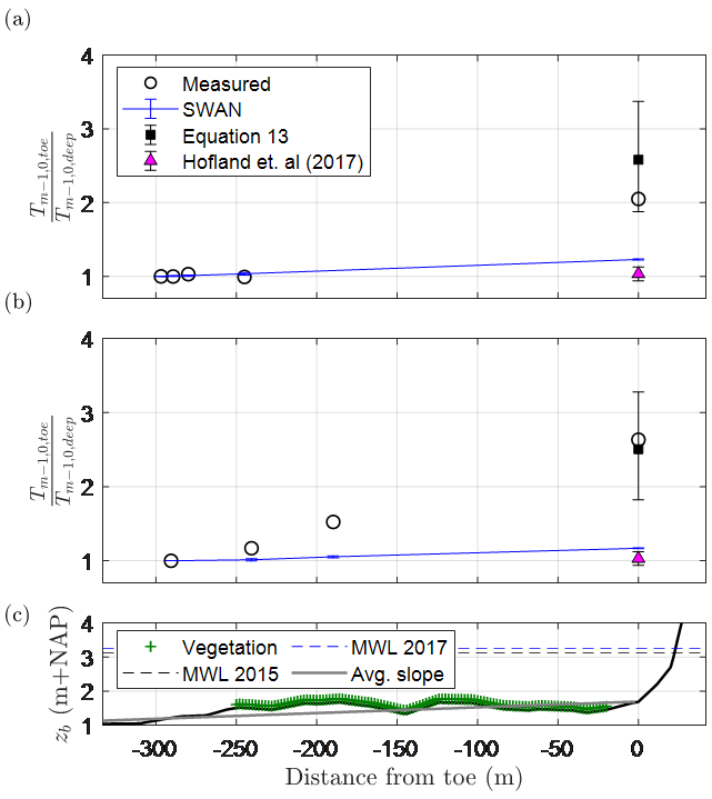
Figure 8 Comparison of measured and modelled relative spectral wave period ($T_{m-\mathrm{1},\mathrm{0},\mathrm{toe}}/T_{m-\mathrm{1},\mathrm{0},\mathrm{deep}}$) at the peaks of the (a) January 2015 and (b) January 2017 storms at Uithuizerwad (see Fig. 5 for gauge locations). Error bars represent the uncertainty in the estimates based on the standard deviations of Eq. (12), Eq. (18) and the Hofland et al. (2017) formula (Appendix C). Panel (c) shows the bed level and vegetated cover. MWL: mean water level (at the peak of the storm).

3.2 Probability of failure: Uithuizerwad case

3.2.1 Influence of IG waves on the probability of failure

Using the full probabilistic framework (Sect. 2.2), the annual probabilities of failure due to wave overtopping (P_f) at Uithuizerwad are presented in Fig. 9a for the two scenarios considered (Sect. 2.2.5) and an additional scenario to assess the influence of standing vegetation. The calculated P_f value is presented alongside estimates of the wave height and period at the toe for a proxy storm with an exceedance probability of $\mathrm{1}/\mathrm{3000}$ per year (Fig. 9b), which is in line with the safety standard.

Figure 9 Relationship between (a) annual failure probabilities at Uithuizerwad for the scenarios considered and (b) physical parameters for a proxy storm with an exceedance probability of $\mathrm{1}/\mathrm{3000}$ per year and a still water level of 5.26 m + NAP. Crest level of 6 m + NAP and dike slope of 1:7 are considered. Note that the influence of vegetation may be overestimated (Sect. 4.4).

Scenario 2 (SS + IG) results in a P_f value 1.3 times larger than that of Scenario 1 (SS) (Fig. 9a). This increase corresponds well with the increase in the spectral wave period at the toe ($T_{m-\mathrm{1},\mathrm{0},\mathrm{toe}}$) and, to a lesser extent, the increase in wave height at the toe ($H_{m_{\mathrm{0}},\mathrm{toe}}$) due to IG waves (Fig. 9b). If the effects of standing vegetation are considered – with (SS + IG + Veg) or without IG waves (SS + Veg) – the P_f value is reduced by 1 order of magnitude (Fig. 9a). This is due to the wave attenuation effect of the vegetation, which reduces both $H_{m_{\mathrm{0}},\mathrm{toe}}$ and $T_{m-\mathrm{1},\mathrm{0},\mathrm{toe}}$ compared to Scenario 1 (SS) or Scenario 2 (SS + IG) alone (Fig. 9b).

3.2.2 Influence of parameter values and uncertainty on the probability of failure

The influence of the dike crest level (z_c) on the calculated P_f value is presented in Fig. 10a. It can be seen that the influence of the IG waves increases with an increasing z_c value. This is because the large load (q_a) needed for failure of a higher dike is reached earlier when IG waves are included. On the other hand, the difference between Scenario 1 and Scenario 2 remains rather constant with varying values for the critical wave overtopping discharge, q_crit, while the magnitude of the calculated P_f value decreases by a factor of O(10) when q_crit is increased by the same magnitude (Fig. 10b).

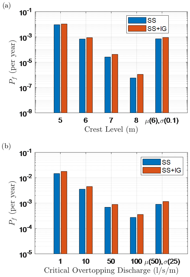
Figure 10 Annual failure probabilities for the two scenarios considered for the following: (a) different dike crest levels with a fixed critical overtopping discharge of 50 L s⁻¹ m⁻¹ and (b) different critical overtopping discharges with a fixed crest level of 6 m + NAP and dike slope of 1:7.

Overall, the results of the validation suggest that Eqs. (12) and (18) may be applied to the area with reasonable accuracy. Likewise, the results of the application of the model framework to the case at Uithuizerwad are in line with expectations. The calculated failure probability for Scenario 1 (SS) is similar to the assumed safety standard (less than $\mathrm{1}/\mathrm{1000}$ per year), and the differences observed between the scenarios show clear relationships with physical wave parameters at the dike toe, namely the significant wave height and spectral wave period that determine the magnitude of wave overtopping (Fig. 9b). With confidence in the model framework, it is applied to the wider Dutch Wadden Sea area (Fig. 1) for a spatial analysis of the P_f value.

3.3 Probability of failure for the wider Wadden Sea area

As a next step, the dikes of the wider Dutch Wadden Sea area are considered from the city of Harlingen to those west of Eemshaven in the city of Groningen. Again, we apply the assumption of a constant dike height of 6 m (above NAP) and a slope of 1:7 for all the dikes in the area. For Scenario 1 (only SS waves), the probability of failure due to wave overtopping ($P_{{\mathrm{f}}_{\mathrm{1}}}$) ranges from $\mathrm{1.1}\times {\mathrm{10}}^{-\mathrm{4}}$ to $\mathrm{3.1}\times {\mathrm{10}}^{-\mathrm{2}}$ per year with an average value of $\mathrm{4.6}\times {\mathrm{10}}^{-\mathrm{3}}$ per year (Fig. 11a). These variations in $P_{{\mathrm{f}}_{\mathrm{1}}}$ are due to the following: (i) the level of exposure, where areas behind inlets are exposed to higher values of $H_{m_{\mathrm{0}},\mathrm{deep}}$ and $T_{m-\mathrm{1},\mathrm{0},\mathrm{deep}}$ compared to those behind the barrier islands; (ii) variations in the mean water level ($\stackrel{\mathrm{‾}}{\mathit{\eta }}$), where values in the west can be approximately 0.5 m lower than those in the east for the same return period event; and (iii) the amount of wave dissipation that occurs due to depth-induced wave breaking over the foreshore, where attenuation is greater at locations with higher foreshore elevations.

Figure 11 Spatial variation in the probability of dike failure by wave overtopping for (a) Scenario 1 of SS ($P_{{\mathrm{f}}_{\mathrm{1}}}$) and (b) Scenario 2 of SS + IG relative to Scenario 1 ($P_{{\mathrm{f}}_{\mathrm{2}}}/P_{{\mathrm{f}}_{\mathrm{1}}}$) across the wider Dutch Wadden Sea area for dikes with identical crest heights (z_c=6 m + NAP) and dike slopes (cot (α)=7).

To explain this further, we examine the variations in $P_{{\mathrm{f}}_{\mathrm{1}}}$ against physical parameters for a proxy storm with an exceedance probability of $\mathrm{1}/\mathrm{3000}$ per year. In Fig. 12a, an offshore forcing parameter ($H_{m_{\mathrm{0}},\mathrm{deep}}^{\mathrm{2}}{T}_{m-\mathrm{1},\mathrm{0},\mathrm{deep}}$), which is proportional to the offshore energy flux, is used to represent the combined influence of $H_{m_{\mathrm{0}},\mathrm{deep}}$ and $T_{m-\mathrm{1},\mathrm{0},\mathrm{deep}}$. In Fig. 12b, the influence of variations in $\stackrel{\mathrm{‾}}{\mathit{\eta }}$ and the bed level at the toe (z_b,toe) are represented by $h_{\mathrm{toe}}=\stackrel{\mathrm{‾}}{\mathit{\eta }}-z_{\mathrm{b},\mathrm{toe}}$. The calculated $P_{{\mathrm{f}}_{\mathrm{1}}}$ value shows a strong positive relationship with $H_{m_{\mathrm{0}},\mathrm{deep}}^{\mathrm{2}}{T}_{m-\mathrm{1},\mathrm{0},\mathrm{deep}}$ (R²=0.65), meaning that higher forcing results in higher failure probabilities. Though the correlation with h_toe is lower (R²=0.43), there is a trend of increasing $P_{{\mathrm{f}}_{\mathrm{1}}}$ with increasing h_toe. This is because larger h_toe (lower z_b,toe) values lead to higher wave heights at the toe due to less wave breaking. Likewise, higher water levels ($\stackrel{\mathrm{‾}}{\mathit{\eta }}$) associated with larger h_toe values also lead to lower freeboards, which results in higher overtopping volumes. Figure 12 also highlights that dikes fronted by mudflats typically have higher $P_{{\mathrm{f}}_{\mathrm{1}}}$ values than those with salt marshes, as salt marshes accrete higher bed levels, which in turn promote more SS-wave attenuation by breaking.

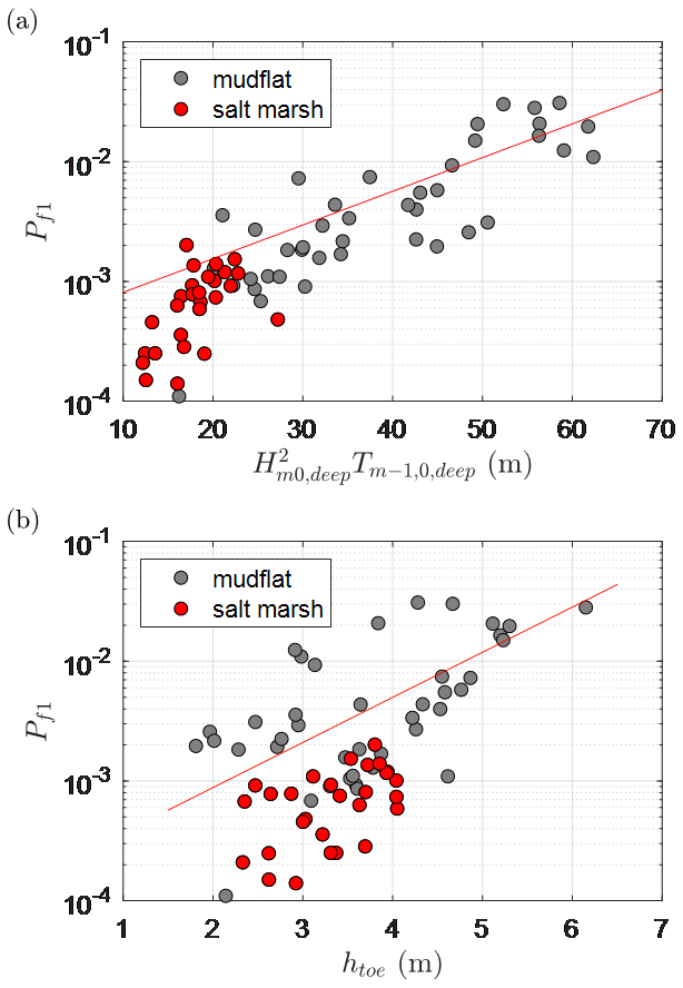
Figure 12 Relationship between the probability of failure for Scenario 1 (SS) and the following: (a) an offshore forcing parameter and (b) the water depth at the dike toe (h_toe), across the wider Dutch Wadden Sea area. Lines indicate the best fit through the data.

In order to identify the influence of the IG waves, the probability of failure by wave overtopping in Scenario 2 relative to that of Scenario 1 ($P_{{\mathrm{f}}_{\mathrm{2}}}{P}_{{\mathrm{f}}_{\mathrm{1}}}$) is assessed. Figure 11b shows that $P_{{\mathrm{f}}_{\mathrm{2}}}/P_{{\mathrm{f}}_{\mathrm{1}}}$ ranges from 1.1 to 1.6, with an average value of 1.2. This increase in P_f is due predominantly to the increase in $T_{m-\mathrm{1},\mathrm{0},\mathrm{toe}}/T_{m-\mathrm{1},\mathrm{0},\mathrm{deep}}$ (at the design point) between Scenario 2 and Scenario 1 – represented by ${\stackrel{\mathrm{̃}}{T}}_{\mathrm{2}}/{\stackrel{\mathrm{̃}}{T}}_{\mathrm{1}}$ (Fig. 13), where $\stackrel{\mathrm{̃}}{T}=T_{m-\mathrm{1},\mathrm{0},\mathrm{toe}}/T_{m-\mathrm{1},\mathrm{0},\mathrm{deep}}$ and subscripts 1 and 2 represent Scenario 1 and Scenario 2, respectively. Figure 13a shows a strong positive relationship between $P_{{\mathrm{f}}_{\mathrm{2}}}/P_{{\mathrm{f}}_{\mathrm{1}}}$ and ${\stackrel{\mathrm{̃}}{T}}_{\mathrm{2}}/{\stackrel{\mathrm{̃}}{T}}_{\mathrm{1}}$ (R²=0.76), where an increase of a factor of 2 in the spectral wave period (${\stackrel{\mathrm{̃}}{T}}_{\mathrm{2}}/{\stackrel{\mathrm{̃}}{T}}_{\mathrm{1}}$) corresponds to an increase of 1.4 times in the failure probability ($P_{{\mathrm{f}}_{\mathrm{2}}}/P_{{\mathrm{f}}_{\mathrm{1}}}$). On the other hand, the increase in wave height at the toe due to the IG waves between the two scenarios (${\stackrel{\mathrm{̃}}{H}}_{\mathrm{2}}/{\stackrel{\mathrm{̃}}{H}}_{\mathrm{1}}$) was negligible (0.5 % to 4.5 %, Fig. 13c) compared to the increase in wave period.

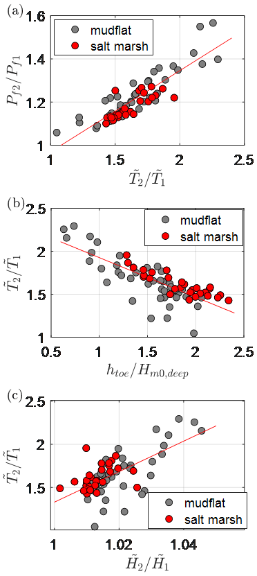
Figure 13 (a) Relationship between the change in probability of failure due to IG waves ($P_{{\mathrm{f}}_{\mathrm{2}}}/P_{{\mathrm{f}}_{\mathrm{1}}}$) and the increase in the relative spectral wave period at the toe (${\stackrel{\mathrm{̃}}{T}}_{\mathrm{2}}/{\stackrel{\mathrm{̃}}{T}}_{\mathrm{1}}$) with the relationship between ${\stackrel{\mathrm{̃}}{T}}_{\mathrm{2}}/{\stackrel{\mathrm{̃}}{T}}_{\mathrm{1}}$ and (b) the relative water depth ($h_{\mathrm{toe}}/H_{m_{\mathrm{0}},\mathrm{deep}}$) and (c) the relative wave height at the toe ($H_{\mathrm{2}}/{\stackrel{\mathrm{̃}}{H}}_{\mathrm{1}}$), across the wider Wadden area. Note that $\stackrel{\mathrm{̃}}{T}$ is a stand-in for $T_{m-\mathrm{1},\mathrm{0},\mathrm{toe}}/T_{m-\mathrm{1},\mathrm{0},\mathrm{deep}}$. Subscripts 1 and 2 refer to Scenario 1 and Scenario 2, respectively.

As $T_{m-\mathrm{1},\mathrm{0},\mathrm{toe}}/T_{m-\mathrm{1},\mathrm{0},\mathrm{deep}}$ depends largely on the offshore wave height, water depth at the toe and foreshore slope (Eq. 18), the spatial variations in $P_{{\mathrm{f}}_{\mathrm{2}}}/P_{{\mathrm{f}}_{\mathrm{1}}}$ (Fig. 11b) are due to variations in local bathymetric and forcing conditions. This is further demonstrated in Fig. 13b by examining the relationship between the increase in the spectral wave period (${\stackrel{\mathrm{̃}}{T}}_{\mathrm{2}}/{\stackrel{\mathrm{̃}}{T}}_{\mathrm{1}}$) and the relative water depth under proxy storm conditions ($\mathrm{1}/\mathrm{3000}$ per year). The relative water depth parameter, which takes into account the variations in both local water depth (h_toe) and offshore wave height ($H_{m_{\mathrm{0}},\mathrm{deep}}$), shows a clear negative relationship with ${\stackrel{\mathrm{̃}}{T}}_{\mathrm{2}}/{\stackrel{\mathrm{̃}}{T}}_{\mathrm{1}}$ (R²=0.61). Therefore, areas with low water depths at the toe relative to large offshore waves are expected to have a greater IG-wave influence on $T_{m-\mathrm{1},\mathrm{0},\mathrm{toe}}$. This is also seen by the areas with a higher IG-wave influence to the west in Fig. 11b, which correspond to points with higher offshore waves (>2.4 m, at the design point) and shallower water depths (<1.4 m), compared to the other locations (with offshore wave heights typically <2 m and water depths at the toe >3 m).

It should be noted that the increase in the spectral wave period due to IG waves is also sensitive to the estimated foreshore slope (Eq. 18). However, ${\stackrel{\mathrm{̃}}{T}}_{\mathrm{2}}/{\stackrel{\mathrm{̃}}{T}}_{\mathrm{1}}$ showed little correlation with the foreshore slope here (R²<0.1), since the foreshores of the Dutch Wadden Sea can all be considered very gentle (1:600, on average).

4 Discussion

4.1 Modelling approach

The combined numerical and empirical approach to wave transformation proved accurate when compared to the 2015 and 2017 storm data at Uithuizerwad, also highlighting the growth of ${\stackrel{\mathrm{̃}}{H}}_{\mathrm{IG}}$ (Fig. 7) and the associated increase in $T_{m-\mathrm{1},\mathrm{0}}/T_{m-\mathrm{1},\mathrm{0},\mathrm{deep}}$ (Fig. 8) as the water depth becomes shallower. Of particular note is the difference in $T_{m-\mathrm{1},\mathrm{0},\mathrm{toe}}/T_{m-\mathrm{1},\mathrm{0},\mathrm{deep}}$ calculated by the phase-averaged wave model SWAN compared to measurements. While the measurement data are likely contaminated by IG waves reflected from the dike, leading to longer wave periods, there is still a gross underestimation of $T_{m-\mathrm{1},\mathrm{0},\mathrm{toe}}/T_{m-\mathrm{1},\mathrm{0},\mathrm{deep}}$ by SWAN due to its exclusion of IG-wave dynamics (Lashley et al., 2020b). Recent works also indicate that the mismatch between the $T_{m-\mathrm{1},\mathrm{0},\mathrm{toe}}/T_{m-\mathrm{1},\mathrm{0},\mathrm{deep}}$ predictions made by SWAN and measurements may be partially explained by its misrepresentation of the frequency dependence of wave dissipation by vegetation (Ascencio, 2020; Jacobsen and McFall, 2019) – where the presence of vegetation significantly influences the shape of the wave spectrum. However, this topic is still under investigation. Despite this underestimation of $T_{m-\mathrm{1},\mathrm{0},\mathrm{toe}}/T_{m-\mathrm{1},\mathrm{0},\mathrm{deep}}$, SWAN was able to accurately model SS-wave transformation over the foreshore (Fig. 6). Likewise, the growth of ${\stackrel{\mathrm{̃}}{H}}_{\mathrm{IG}}$ (Fig. 7) and $T_{m-\mathrm{1},\mathrm{0}}/T_{m-\mathrm{1},\mathrm{0},\mathrm{deep}}$ (Fig. 8) at the dike toe are accurately captured using Eqs. (12) and (18), respectively.

The probabilistic method FORM was able to compute the P_f value within 20 to 30 iterations with a computation time of under 10 min per dike section. Other methods, such as crude Monte Carlo or numerical integration are known to be much more computationally demanding. However, other approaches such as Adaptive Directional Importance Sampling (Den Bieman et al., 2014) may also prove to be equally suitable for this application. This short computation time is also attributed to the use of a phase-averaged wave model (SWAN), which is roughly 100 times faster than its phase-resolving counterparts (e.g. SWASH – Simulating WAves till SHore – or XBeach non-hydrostatic) (Lashley et al., 2020b).

As the dike characteristics (crest level, slope and critical overtopping discharge) typically dominate the probabilistic analysis, their treatment as deterministic variables here allowed for the analysis to focus on the influence of foreshore parameters. Furthermore, by treating the influence of the IG waves as a separate module (Sect. 2.2.2), calculations with and without IG waves could be easily performed. Such a modular approach allows for the framework to be easily modified or adapted to varying conditions. For example, the module to calculate the actual overtopping discharge could be extended with the formulae of Lashley et al. (2021) for environments where the conditions at the structure toe are extremely shallow or in the case of vertical seawalls rather than sloping structures. Likewise, another numerical or empirical model more suited to the specific area of application could replace the model used here for SS-wave transformation (SWAN). This makes the overall approach easily adaptable and applicable to other coastlines where IG waves may play a critical role, such as the Belgian coast (Altomare et al., 2016), Japanese coast (Mase et al., 2013), and northern and southern coasts of Vietnam (Nguyen et al., 2020).

To account for the error in the empirical models, the estimates were multiplied by normally distributed factors with mean values and standard deviations to represent the bias and scatter (errors) associated with each model (Section 2.2). This uncertainty was also shown in Figs. 6 to 8 as error bars. As the overall approach is a succession of different numerical and empirical models, it is important to note the combined error. The combined error (or uncertainty) may be expressed using a coefficient of variation, which is equal to the combined standard deviation normalized by the combined mean. If we consider the means and standard deviations of Eqs. (4), (12), (18) and (19), the combined coefficient of variation or uncertainty is 0.15 or 15 %.

4.2 Applicability of formulae for the actual overtopping discharge

In the present study, the original overtopping formula of Van Gent (1999) (Eq. 19) was applied to all locations. This formula was selected because it was developed specifically for shallow foreshores considering the influence of both SS and IG waves and is considered valid for a wide range of breaker parameter (${\mathit{\xi }}_{m-\mathrm{1},\mathrm{0}}$) values. However, applying Eq. (19) here – to locations with ${\mathit{\xi }}_{m-\mathrm{1},\mathrm{0}}<\mathrm{5}$ at the design point – does not coincide with the current European standard (EurOtop, 2018). In EurOtop (2018), different formulae are applied depending on the ${\mathit{\xi }}_{m-\mathrm{1},\mathrm{0}}$ value (Van der Meer and Bruce, 2014; Altomare et al., 2016). An analysis of the different approaches revealed the following points:

• For ${\mathit{\xi }}_{m-\mathrm{1},\mathrm{0}}<\mathrm{1.8}$, which is typical for cot (α)=7, the spectral wave period showed a considerable influence on the overtopping discharge (q_a) calculated using the EurOtop (2018) approach. Figure 14a shows that an increase of 1.5 times in wave period (due to IG waves) (${\stackrel{\mathrm{̃}}{T}}_{\mathrm{2}}/{\stackrel{\mathrm{̃}}{T}}_{\mathrm{1}}$) resulted in an order of magnitude increase of P_f using the EurOtop (2018) approach. Since the EurOtop (2018) formula for ${\mathit{\xi }}_{m-\mathrm{1},\mathrm{0}}<\mathrm{1.8}$ (Van der Meer and Bruce, 2014) was not derived for shallow foreshore conditions (with IG waves), this significant increase in the P_f value is likely incorrect and requires further research.

• For $\mathrm{1.8}<{\mathit{\xi }}_{m-\mathrm{1},\mathrm{0}}<\mathrm{5}$, which is typical for cot (α)=3, the wave period no longer influences the EurOtop (2018) calculation, as a maximum q_a value is reached. This is evident in Fig. 14b, as no clear trend between ${\stackrel{\mathrm{̃}}{T}}_{\mathrm{2}}/{\stackrel{\mathrm{̃}}{T}}_{\mathrm{1}}$ and $P_{{\mathrm{f}}_{\mathrm{2}}}/P_{{\mathrm{f}}_{\mathrm{1}}}$ is visible for the EurOtop (2018) calculations. In these cases, the differences between EurOtop (2018) and the original Van Gent (1999) calculations are much smaller (Fig. 14).

• For ${\mathit{\xi }}_{m-\mathrm{1},\mathrm{0}}>\mathrm{7}$ or wave steepness at the toe less than 0.01, the modified version of the Van Gent (1999) formula based on an equivalent slope concept (Altomare et al., 2016) and described in EurOtop (2018) is only applicable to foreshore slopes steeper than or equal to 1:250. As the foreshore slopes of the Wadden Sea are typically gentler than 1:500, the modified formulae could not be used here. Therefore, locations meeting these criteria were excluded for the EurOtop (2018) calculations.

• The results using the original Van Gent (1999) formula were of the same order of magnitude for both dike slopes considered (Fig. 14), suggesting that the formula was not very sensitive to changes in ${\mathit{\xi }}_{m-\mathrm{1},\mathrm{0}}$. However, it should be noted that this formula was derived using a limited dataset with cot (α) values of 2.5 and 4 and cot (m) values of 100 and 250. Therefore, future studies should verify its performance for conditions with values of cot (α)>4 and cot (m)>250.

The above findings suggest that the EurOtop (2018) approach may be incorrect for shallow foreshore conditions with gentle dike slopes (e.g. 1:7), which often have ${\mathit{\xi }}_{m-\mathrm{1},\mathrm{0}}<\mathrm{1.8}$. The source of this uncertainty lies in the sensitivity of the formulae to $T_{m-\mathrm{1},\mathrm{0},\mathrm{toe}}$, a parameter whose magnitude increases proportionally with the magnitude of the IG waves (Eq. 18, Fig. C2). As Oosterlo et al. (2018) applied the EurOtop (2007) formulae to a dike with an average slope of 1:8, it can be concluded that the large influence of the IG waves – where including IG waves increased the failure probability by 10³ – reported by the authors was indeed due to the method used.

Table 4 Results of XBeach non-hydrostatic simulations taken at the dike toe for two different foreshore slopes under the same offshore forcing conditions ($H_{m_{\mathrm{0}},\mathrm{deep}}=\mathrm{1}$ m, $T_{m-\mathrm{1},\mathrm{0},\mathrm{deep}}=\mathrm{4.54}$ s and h_toe=1 m).

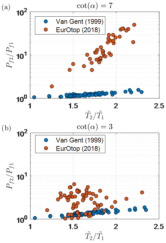
Figure 14 Relationship between the change in probability of failure due to IG waves ($P_{{\mathrm{f}}_{\mathrm{2}}}/P_{{\mathrm{f}}_{\mathrm{1}}}$) and the increase in the relative spectral wave period at the toe (${\stackrel{\mathrm{̃}}{T}}_{\mathrm{2}}/{\stackrel{\mathrm{̃}}{T}}_{\mathrm{1}}$) calculated using the original Van Gent (1999) and EurOtop (2018) approaches for the actual overtopping discharge for (a) cot (α)=7 and (b) cot (α)=3. Note that cases with wave steepness at the toe < 0.01 were excluded from the EurOtop (2018) calculations, since the equivalent slope concept could not be applied (Sect. 4.2).

4.3 Influence of IG waves on design parameters

The influence of IG waves may be represented as an increase in the magnitude of both design parameters ($H_{m_{\mathrm{0}},\mathrm{toe}}$ and $T_{m-\mathrm{1},\mathrm{0},\mathrm{toe}}$), compared to a situation where the IG waves are neglected. This was demonstrated by Lashley et al. (2020b), where the relative magnitude of the IG waves $({\stackrel{\mathrm{̃}}{H}}_{\mathrm{IG}}=H_{m_{\mathrm{0}},\mathrm{IG},\mathrm{toe}}/H_{m_{\mathrm{0}},\mathrm{SS},\mathrm{toe}})>\mathrm{0.5}$ had a notable influence on both parameters. In the present study, ${\stackrel{\mathrm{̃}}{H}}_{\mathrm{IG}}$ was much lower, ranging from 0.14 to 0.35 with a mean value of 0.19 (considering proxy storm conditions with $\mathrm{1}/\mathrm{3000}$ per year exceedance probability). As a result, the impact of the IG waves on the total wave height at the toe was negligible (0.5 % to 4.5 %), since $H_{m_{\mathrm{0}},\mathrm{toe}}=\sqrt{H_{m_{\mathrm{0}},\mathrm{IG},\mathrm{toe}}^{\mathrm{2}}+H_{m_{\mathrm{0}},\mathrm{SS},\mathrm{toe}}^{\mathrm{2}}}$. That said, there was still a notable increase in $T_{m-\mathrm{1},\mathrm{0},\mathrm{toe}}$. This is attributed to the following: (i) the sensitivity of $T_{m-\mathrm{1},\mathrm{0}}$ to wave energy density at low frequencies, by definition (Eq. 9), and (ii) the influence of the foreshore slope on the shape of the wave spectrum at the toe – where gentler foreshore slopes lead to wider surf zones and more energy transfer to lower frequencies. This makes $T_{m-\mathrm{1},\mathrm{0},\mathrm{toe}}$ more sensitive to very gentle foreshore slopes compared to the ${\stackrel{\mathrm{̃}}{H}}_{\mathrm{IG}}$ parameter alone (Appendix C). This is further demonstrated in Fig. 15 using the results of two numerical simulations (XBeach non-hydrostatic). The increase in $T_{m-\mathrm{1},\mathrm{0},\mathrm{toe}}$ due to IG waves is larger for the 1:500 foreshore slope than the one of 1:50, despite having similar ${\stackrel{\mathrm{̃}}{H}}_{\mathrm{IG}}$ values (Fig. 15, Table 4). Table 4 also highlights that while the influence of the IG waves on $T_{m-\mathrm{1},\mathrm{0},\mathrm{toe}}$ is noteworthy, their influence on the total wave height at the toe ($H_{m_{\mathrm{0}},\mathrm{toe}}$) is negligible.

Figure 15 Results of XBeach non-hydrostatic numerical simulations showing wave spectra at the dike toe for a 1:50 and 1:500 foreshore slope, under the same offshore forcing conditions ($H_{m_{\mathrm{0}},\mathrm{deep}}=\mathrm{1}$ m, $T_{m-\mathrm{1},\mathrm{0},\mathrm{deep}}=\mathrm{4.54}$ s and h_toe=1 m). Dashed vertical line indicates the frequency separating IG- and SS-wave motions.

The main takeaway here is that while IG waves may have a negligible influence on the design wave height at the structure, their influence on the design wave period can be considerable and should therefore not be neglected, particularly on gentle foreshore slopes.

4.4 Influence of salt marsh vegetation

Another discussion point is the influence of salt marsh vegetation and whether its effects should be considered for very high return period events. Figure 9 suggests that safety could be significantly improved by standing salt marsh vegetation; however, these findings must be interpreted with caution. In their analysis based on dikes with foreshores in the Wadden Sea, Vuik et al. (2018b) included a stem-breakage model and concluded that it was very likely that almost all vegetation would break at this location under extreme forcing – resulting in P_f values similar to that of non-vegetated foreshores. This flattening and breaking of salt marsh vegetation under storm conditions was also reported by Möller et al. (2014), who conducted large-scale flume experiments with transplanted Wadden Sea vegetation. Moreover, though the vegetation component of Eq. (12) was able to capture the influence of vegetation on IG waves for the two storms considered here (Figs. 6 to 8), its performance for more extreme events requires further validation. This is due to the low ratio of stem height to water depth ($h_{\mathrm{toe}}/h_{\mathrm{v}}=\mathrm{3.3}$) considered in its derivation. As a result, Eq. (12) may overestimate the influence of vegetation for high return period events with $h_{\mathrm{toe}}/h_{\mathrm{v}}\approx \mathrm{13}$. Thus, the influence of salt marsh vegetation on coastal safety under extreme forcing remains an important issue for future research.

4.5 Implications for practice

Including the effects of IG waves (Scenario 2) increases of P_f by up to 1.6 times, compared to Scenario 1 (Figs. 9 and 11b). This effect is considerably smaller than that reported by Oosterlo et al. (2018), where including the IG waves increased the P_f value by 3 orders of magnitude. Results here suggest that Oosterlo et al. (2018) likely overestimated the influence of the IG waves due to an inappropriate use of empirical overtopping formulae that were not formulated specifically for situations with IG waves (Van der Meer, 2002; EurOtop, 2007), as demonstrated in Sect. 4.2. But what does the presence of IG waves mean for practice? In general, the reliability of the existing defences may be overestimated, since IG waves are largely neglected in their assessment. By interpolating the results of Fig. 10 logarithmically, the required crest level at Uithuizerwad for a fixed target probability of failure can be determined. For a target annual failure probability of $\mathrm{1}/\mathrm{1000}$ per year (which corresponds to the safety standard), a crest level of 6.3 m (+ NAP) is needed for Scenario 1 (SS). For Scenario 2 (SS + IG), the required crest level is 6.5 m. Therefore, the influence of the IG waves may be alternatively seen as an increase in the required crest level of around 0.2 m with a cost of the order of magnitude of EUR 1 million per kilometre (Jonkman et al., 2013). If the influence of the IG waves on the P_f value were 1 order of magnitude larger, as suggested by the EurOtop (2018) formula (Fig. 14a), then the increase in the required crest level would be around 0.8 m with an order of magnitude increase in cost (EUR 10 million per kilometre).

This increase in P_f is attributed to the growth of $T_{m-\mathrm{1},\mathrm{0},\mathrm{toe}}$ due to the IG waves and the well-known relationship between wave overtopping and wave period, where longer waves (larger $T_{m-\mathrm{1},\mathrm{0},\mathrm{toe}}$ values) result in more overtopping (Sect. 2.2.3) and, by extension, higher P_f values. These findings suggest that attention should also be given to changes in wave period – and not to wave height attenuation alone – when considering the influence of shallow foreshores on safety. However, it is important to stress that this effect is highly dependent on local conditions, as $T_{m-\mathrm{1},\mathrm{0},\mathrm{toe}}/T_{m-\mathrm{1},\mathrm{0},\mathrm{deep}}$ (Eq. 18) is dependent on the offshore wave height, the water depth at the toe and the estimated foreshore slope. Therefore, it should be assessed on a case-by-case basis rather than assumed constant over a large area. This spatial variability is demonstrated in Fig. 11b. Additionally, the calculated $P_{{\mathrm{f}}_{\mathrm{2}}}$ value was found to be somewhat sensitive to the uncertainty in Eqs. (12) and (18) (Appendix D), which are based primarily on numerical simulations, since field and physical model data are lacking. Future studies should carry out experiments to further validate and improve the empirical formulations presented here and, if possible, reduce the uncertainty (scatter) in their estimates.

Even though vegetation itself was neglected in the probabilistic analysis of the wider Wadden Sea area, findings here still advocate for the importance of maintaining salt marshes. As (higher) salt marshes trap sediment, their raised platforms attenuate more SS waves than lower mudflats, which results in lower P_f values – even when IG waves are taken into account (Fig. 16). These findings support the arguments of Zhu et al. (2020) for the net positive impact of shallow foreshores on coastal safety. However, the estimated increase in safety due to the foreshore may be reduced when IG waves are included in the analysis – in particular where wave overtopping is concerned. In planning and implementing foreshore systems, it is therefore important to consider the effects of IG waves on safety as well.

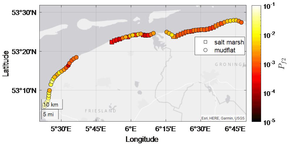
Figure 16 Influence of raised bed levels due to salt marshes on the spatial variation in the probability of dike failure by wave overtopping for Scenario 2: SS + IG waves ($P_{{\mathrm{f}}_{\mathrm{2}}}$) across the wider Dutch Wadden Sea area for dikes with identical crest heights (z_c=6 m + NAP) and dike slopes (cot (α)=7).

5 Conclusion

By combining several numerical and empirical models, the influence of infragravity (IG) waves on the probability of dike failure by wave overtopping (P_f) was quantified for a shallow intertidal area: the Dutch Wadden Sea. The model framework was first validated for a single location using data collected during two storms, each with exceedance probabilities of approximately $\mathrm{1}/\mathrm{5}$ per year. The approach accurately estimated the effects of shallow foreshores on wave propagation, namely (i) the dissipation of incident SS waves by depth-induced breaking, (ii) the increase in the relative magnitude of the IG waves (${\stackrel{\mathrm{̃}}{H}}_{\mathrm{IG}}$) and (iii) the increase in the relative spectral wave periods ($T_{m-\mathrm{1},\mathrm{0}}/T_{m-\mathrm{1},\mathrm{0},\mathrm{deep}}$). The framework was then applied to the wider Dutch Wadden Sea for a spatial analysis. Including the IG waves increased the P_f value by a factor of 1.1 to 1.6, suggesting that safety is indeed overestimated when they are neglected. This increase is attributed to the influence of the IG waves on the design wave period and, to a lesser extent, the wave height at the dike toe. The spatial variation in this effect, observed for the case considered, highlights its dependence on local conditions – with IG waves showing greater influence at locations with larger offshore waves, such as those behind tidal inlets, and shallower water depths.

For the mild dike slope considered (1:7), the change in P_f due to the IG waves showed high sensitivity to the empirical wave overtopping model applied – where the use of a model that was not developed for shallow foreshores and IG waves (EurOtop, 2018) resulted in failure probabilities up to 55 times higher compared to a method from Van Gent (1999). It is thus important that practitioners consider both the impact of IG waves and the appropriateness of the models used when assessing flood risk along coastlines with shallow foreshores. The methods proposed in this paper can aid in this by allowing practitioners to quickly identify areas where IG waves – and therefore tools which account for them – should be included in the analysis. Furthermore, given the modular characteristic of the approach, it could be easily fitted with different tools or adapted to other coastlines where IG waves may play a significant role. Examples of such sites include the sandy foreshores along the Belgian coast (Altomare et al., 2016); the wide shelves of the Mekong Delta, Vietnam (Nguyen et al., 2020); and the steep foreshores found in Japan (Mase et al., 2013).

Despite the utility of the proposed approach and importance of the findings herein, the results are subject to certain limitations. For instance, the analysis was conducted assuming a fixed dike height with a uniform slope at each location. Therefore, it is recommended that the analysis be repeated using the actual dike geometries where the crest level is notably higher, as findings here suggest that the influence of the IG waves would likely be higher (Fig. 10a). Furthermore, we have validated and applied the framework to a shallow intertidal area, but it is recommended that the framework be applied to sites with different hydrodynamic and geomorphological features, such as open coasts or those fronted by coral reefs. It must also be noted that the current study did not consider edge or leaky (free) IG waves (Reniers et al., 2021). Therefore, additional field campaigns focused on measuring IG waves are recommended to determine the contribution, if any, of free IG waves to wave conditions in the Dutch Wadden Sea. Finally, while vegetation had a notable influence on wave attenuation for storms with a relatively high probability of exceedance ($\mathrm{1}/\mathrm{5}$ per year, Fig. 6), it was assumed to be flattened or broken under more extreme conditions (Vuik et al., 2018a). Further research is required to assess the attenuation effects of salt marsh vegetation under extreme water level and wave forcing.

Appendix A: Overview of stochastic variables

Table A1 Extreme parameters for offshore wave and water level characteristics (Weibull distributions). Note that the scale (sc) and shape (sh) parameters, derived from Hydra-NL estimates, are dependent on location along the Wadden coast; the range of values is provided here.

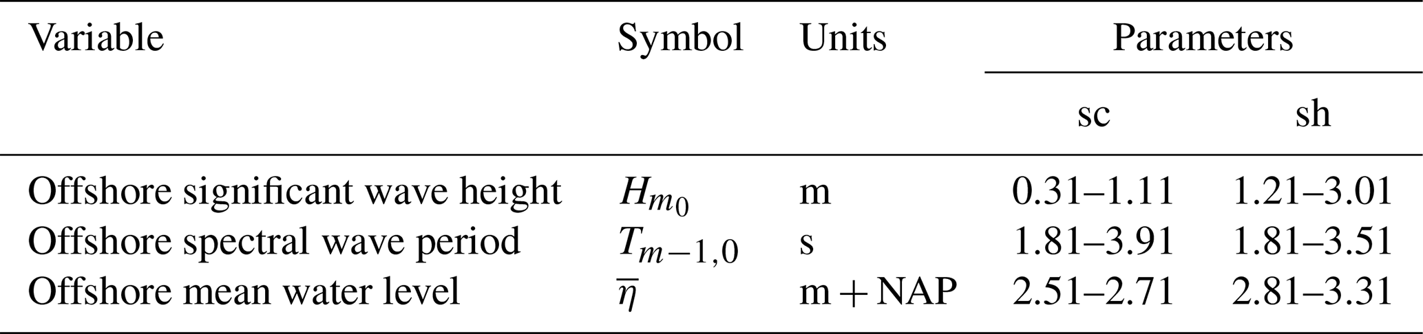
Table A2 Normally distributed foreshore parameters. Note that the mean value (μ^*) is dependent on location along the Wadden coast.

Appendix B: Wave spectra at Uithuizerwad (Wadden Sea) during 2015 and 2017 storms

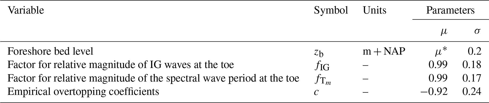
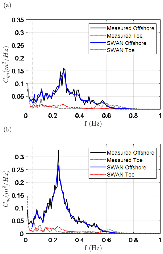
Figure B1 Comparison of observed and modelled wave spectra for (a) January 2015 and (b) January 2017. Dashed vertical lines separate SS and IG frequencies. (See Fig. 5 for reference to instrument locations.)

Appendix C: Derivation of formulae for the spectral wave period at the toe

Hofland et al. (2017) showed that the ratio of the spectral wave period at the structure toe to its deep-water equivalent ($T_{m-\mathrm{1},\mathrm{0},\mathrm{toe}}/T_{m-\mathrm{1},\mathrm{0},\mathrm{deep}}$) may be empirically modelled as a function of relative water depth and foreshore slope (Eqs. C1 to C3). For long-crested waves (no directional spreading), this is

$$\begin{array}{}\text{(C1)}& {\displaystyle \frac{T_{m-\mathrm{1},\mathrm{0},\mathrm{toe},\mathrm{in}}}{T_{m-\mathrm{1},\mathrm{0},\mathrm{deep}}}}-\mathrm{1}=\mathrm{6}\cdot \exp (-\mathrm{4}\stackrel{\mathrm{̃}}{h})+\exp (-\stackrel{\mathrm{̃}}{h}),\end{array}$$

and for cases with short-crested wave, it is

$$\begin{array}{}\text{(C2)}& {\displaystyle \frac{T_{m-\mathrm{1},\mathrm{0},\mathrm{toe},\mathrm{in}}}{T_{m-\mathrm{1},\mathrm{0},\mathrm{deep}}}}-\mathrm{1}=\mathrm{6}\cdot \exp (-\mathrm{6}\stackrel{\mathrm{̃}}{h})+\mathrm{0.25}\cdot \exp (-\mathrm{0.75}\stackrel{\mathrm{̃}}{h}),\end{array}$$

where

$$\begin{array}{}\text{(C3)}& \stackrel{\mathrm{̃}}{h}={\displaystyle \frac{h_{\mathrm{toe}}}{H_{m_{\mathrm{0}},\mathrm{deep}}}}{\left({\displaystyle \frac{\cot {\mathit{\alpha }}_{\mathrm{fore}}}{\mathrm{100}}}\right)}^{\mathrm{0.2}}.\end{array}$$

However, as Eqs. (C1) to (C3) were based on tests with $\mathrm{35}\le \cot {\mathit{\alpha }}_{\mathrm{fore}}\le \mathrm{250}$, they tend to over- and underestimate $T_{m-\mathrm{1},\mathrm{0},\mathrm{toe}}$ for steep (cot α_fore<35) and very gentle slopes (cot α_fore>250), respectively, with R²=0.30 when applied to the numerical dataset (Fig. C1).

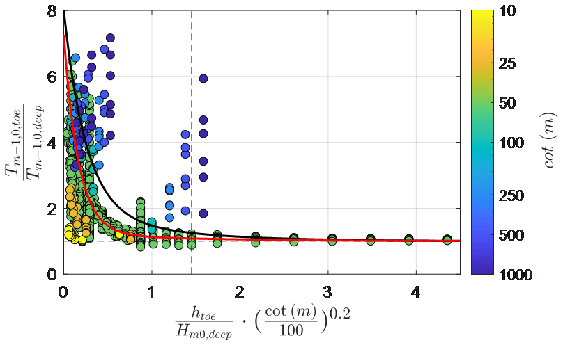
Figure C1 Numerically modelled relative spectral wave period as a function of relative water depth and foreshore slope, following Hofland et al. (2017). Black and red lines represent Eqs. (C1) and (C2), respectively.

This inaccuracy, particularly for very gentle slopes (cot α_fore>250), has also been reported by Nguyen et al. (2020) and suggests that a new formulation is required for application to the Dutch Wadden Sea – where foreshore slopes are typically 1:500 or gentler.

Since both $T_{m-\mathrm{1},\mathrm{0},\mathrm{toe}}$ and ${\stackrel{\mathrm{̃}}{H}}_{\mathrm{IG}}$ describe the amount of energy in the IG band compared to the SS band, it stands to reason that a simple relation should exist between the two parameters. From the Lashley et al. (2020a) numerical dataset, it can be seen that $T_{m-\mathrm{1},\mathrm{0},\mathrm{toe}}{T}_{m-\mathrm{1},\mathrm{0},\mathrm{deep}}$ increases with increasing ${\stackrel{\mathrm{̃}}{H}}_{\mathrm{IG}}$ (R²=0.76) but with scatter related to the foreshore slope (Fig. C2a). Based on these trends, the following relation is proposed:

$$\begin{array}{}\text{(C4)}& {\displaystyle \frac{T_{m-\mathrm{1},\mathrm{0},\mathrm{toe}}}{T_{m-\mathrm{1},\mathrm{0},\mathrm{deep}}}}=\left\{\begin{array}{ll}\mathrm{1.59}\cdot {\stackrel{\mathrm{̃}}{H}}_{\mathrm{IG}}^{\mathrm{0.69}}\cdot {\left(cot{\mathit{\alpha }}_{\mathrm{fore}}\right)}^{\mathrm{0.17}}& \frac{h_{\mathrm{toe}}}{H_{m_{\mathrm{0}},\mathrm{deep}}}\le \mathrm{1}\\ \mathrm{1}& \frac{h_{\mathrm{toe}}}{H_{m_{\mathrm{0}},\mathrm{deep}}}>\mathrm{1}\end{array}\right.,\end{array}$$

where the exponents were determined empirically, by minimizing scatter. Including the foreshore slope term significantly reduces the scatter in the data (R²=0.92, Fig. C2b) and gives a better representation for mild slopes. This is due to the influence of the foreshore slope, not only on the relative magnitude of the IG waves – as already accounted for in Eq. (12) – but also on the spectral shape. As the area over which shoaling occurs increases with gentler foreshore slopes, energy transfer by nonlinear (difference) triad interactions occurs over a longer duration than on steeper slopes. This causes the spectral peak to migrate to lower frequencies and results in larger values of $T_{m-\mathrm{1},\mathrm{0},\mathrm{toe}}$ for gentler foreshore slopes (Battjes, 2004), despite having similar ${\stackrel{\mathrm{̃}}{H}}_{\mathrm{IG}}$ values.

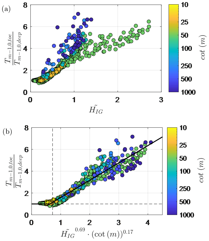
Figure C2 Numerically modelled relative spectral wave period as a function of (a) ${\stackrel{\mathrm{̃}}{H}}_{\mathrm{IG}}$ alone and (b) ${\stackrel{\mathrm{̃}}{H}}_{\mathrm{IG}}$ and an additional foreshore slope term. Solid line represents Eq. (C4). Dashed vertical line indicates $h_{\mathrm{toe}}/H_{m_{\mathrm{0}},\mathrm{deep}}=\mathrm{1}$, and dashed horizontal line represents the deep-water limit, where $T_{m-\mathrm{1},\mathrm{0},\mathrm{toe}}/T_{m-\mathrm{1},\mathrm{0},\mathrm{deep}}\approx \mathrm{1}$.

It should also be noted that for deep-water cases, where $h_{\mathrm{toe}}/H_{m_{\mathrm{0}},\mathrm{deep}}>\mathrm{1}$, $T_{m-\mathrm{1},\mathrm{0},\mathrm{toe}}/T_{m-\mathrm{1},\mathrm{0},\mathrm{deep}}\approx \mathrm{1}$ and is independent of the foreshore slope and ${\stackrel{\mathrm{̃}}{H}}_{\mathrm{IG}}$ parameters (Fig. C2b). This is consistent with the findings of Lashley et al. (2021) which suggest that the foreshore's influence only becomes significant for cases with $h_{\mathrm{toe}}/H_{m_{\mathrm{0}},\mathrm{deep}}\le \mathrm{1}$.

Appendix D: Analysis of sensitivity factors for the Uithuizerwad case

With respect to the stochastic parameters, the sensitivity of the calculated P_f value to uncertainties in each parameter is assessed using the FORM α_sf values (Sect. 2.2.4, Fig. D1). Negative α_sf values represent variables that contribute to the load by increasing the actual overtopping discharge (q_a). In both scenarios, the uncertainty in the offshore water level ($\stackrel{\mathrm{‾}}{\mathit{\eta }}$) dominates the probability of failure with $\mathit{\alpha }\le -\mathrm{0.96}$. This is expected, since the dike is unlikely to fail without extreme water levels (i.e. a severe storm). In Scenario 1 (Fig. D1a), the variables that also contribute to the load are the following: the empirical wave overtopping coefficient (c), since larger c values increase q_a (Sect. 2.2.3); the SWAN breaker parameters (γ_BJ), which controls the magnitude of breaking waves such that higher γ_BJ leads to larger wave heights at the structure toe and thus larger q_a; and the offshore wave forcing parameters ($H_{m_{\mathrm{0}},\mathrm{deep}}$ and $T_{m-\mathrm{1},\mathrm{0},\mathrm{deep}}$).

As expected, when the influence of the IG waves is included in the analysis (Scenario 2, Fig. D1b) the uncertainty in factors for the relative IG-wave height, $f_{\mathrm{IG}}(\mathit{\alpha }=-\mathrm{0.03}$), and spectral wave period, $f_{\mathrm{TM}}(\mathit{\alpha }=-\mathrm{0.02}$), also contribute to the load, as larger $H_{m_{\mathrm{0}},\mathrm{toe}}$ and $T_{m-\mathrm{1},\mathrm{0},\mathrm{toe}}$ values increase q_a. This suggests that the calculated P_f value is indeed sensitive to the accuracy of Eqs. (12) and (18). The uncertainty in the bed level (z_b) also contributes to the load due to its influence on the water depth at the toe, which directly influences the relative magnitude of the IG waves at the dike toe (${\stackrel{\mathrm{̃}}{H}}_{\mathrm{IG}}$).

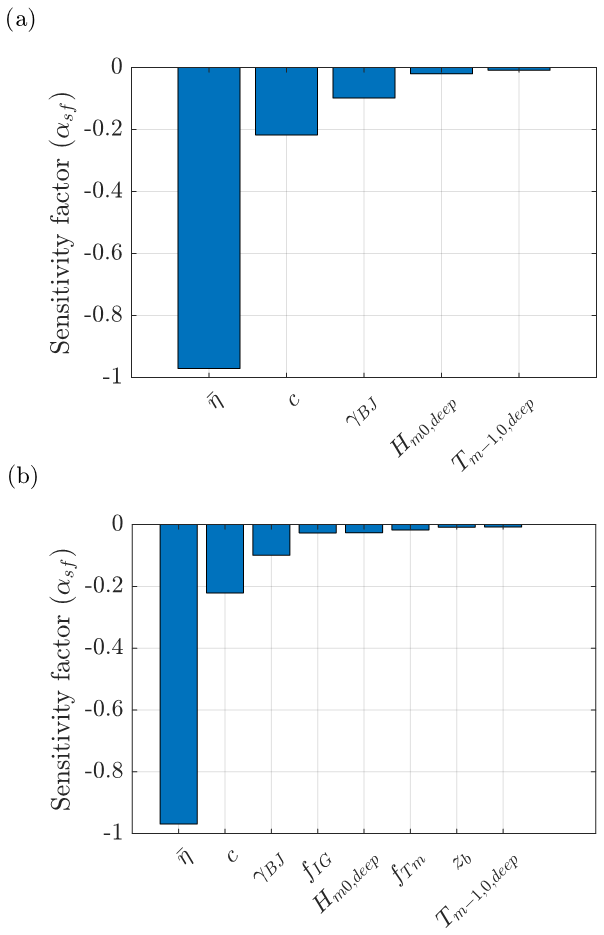
Figure D1 Sensitivity factors (α_sf) ranked from left to right in order of importance, for (a) Scenario 1 of SS and (b) Scenario 2 of SS + IG. Negative values indicate load parameters.