the Creative Commons Attribution 4.0 License.
the Creative Commons Attribution 4.0 License.
 | 10 Mar 2021
A statistical–parametric model of tropical cyclones for hazard assessment
William C. Arthur
We present the formulation of an open-source, statistical–parametric model of tropical cyclones (TCs) for use in hazard and risk assessment applications. The model derives statistical relations for TC behaviour (genesis rate and location, intensity, speed and direction of translation) from best-track datasets, then uses these relations to create a synthetic catalogue based on stochastic sampling, representing many thousands of years of activity. A parametric wind field, based on radial profiles and boundary layer models, is applied to each event in the catalogue that is then used to fit extreme-value distributions for evaluation of return period wind speeds. We demonstrate the capability of the model to replicate observed behaviour of TCs, including coastal landfall rates which are of significant importance for risk assessments.
- Article
(12540 KB) - Full-text XML
- BibTeX
- EndNote


The author's copyright for this publication is transferred to the Commonwealth of Australia (Geoscience Australia) 2020.
Tropical cyclones (TCs) present a significant physical and economic threat to Australian communities. Around 20 % of reported costs from natural disasters arise from TCs (Handmer et al., 2016), while over 30 % of insured loss is caused by TCs (Chen, 2004), due to extreme winds and riverine and coastal storm surge flooding. Minimising the losses in the built environment from these events can be approached in a range of ways. In Australia, the Wind Loading Standard (AS/NZS 1170.2, 2011) specifies minimum design loads for buildings under the action of wind loading. Design loads vary across the country, depending on the sources and magnitude of winds, in an effort to minimise average annual losses across the country. Areas around the northern coastline have higher design loads, due to the exposure to TCs which generate higher wind speeds than mid-latitude storms. Design criteria are defined with reference to a likelihood of exceedance over the expected lifetime of residential structures – this is a 10 % likelihood in 50 years, commonly described as an (approximately) 1-in-500-year average recurrence interval (ARI).
The historical record of TCs in the Australian region covers barely 100 years (Kuleshov et al., 2010). Of that record, only the last 30 years includes reasonably consistent information based on satellite data to assess the intensity of TCs. The short length of record makes it difficult to infer ARI wind speeds due to TCs at ARIs greater than 100 years (Emanuel and Jagger, 2010; Jagger and Elsner, 2006; Sanabria and Cechet, 2007). It is a common approach to use stochastic simulations to estimate the wind speeds to establish building design standards and for assessing TC risk (Vickery et al., 2009). Many of these models exploit the statistical characteristics of TC behaviour to generate catalogues of synthetic events (Emanuel et al., 2006; Hall and Jewson, 2007; James and Mason, 2005; Li and Hong, 2014; Nakajo et al., 2014; Powell et al., 2005; Rumpf et al., 2007).
In this vein, Geoscience Australia has developed a statistical–parametric model of TC behaviour – called the Tropical Cyclone Risk Model (TCRM) – to generate synthetic-event sets that represent many thousands of years of TC activity. TCRM is designed to run on desktop computers with modest computational resources available but is scalable to large multi-processor systems. As such, the model forgoes the more computationally intensive dynamical approach used in some TC hazard models (Emanuel et al., 2006). Instead, we use an autoregressive process to model synthetic TC tracks, including intensity, and use a two-dimensional parametric model to describe the TC wind field.
TCRM is unique in that it is freely available for use in hazard and risk assessment applications. There are a number of published stochastic models (noted above); however these models are, as a general rule, not publicly available (exceptions include the model of Powell et al., 2005) or free. Further, the formulation of these models may preclude application in regions other than those demonstrated in publications. That is, they may be tailored to the region where they are applied. TCRM is formulated such that it is largely independent of the region being simulated, though some components are derived using regionally specific data. Where there are region-specific formulations in a component of the model, these can be readily adapted for different regions. TCRM is also an open-source software package, enabling users to contribute to ongoing development of the model and influence the future directions of development priorities.
While the primary purpose for developing the model is to evaluate TC severe wind hazard, it can be configured to rapidly evaluate the swath of destructive winds from a single TC at a high temporal and spatial resolution. In this configuration, a two-dimensional wind field at a 0.02∘ horizontal resolution, covering the entire track of a TC, is calculated in a matter of minutes. Using TCRM in this manner, we have evaluated the impact of individual TCs on Australian communities, with applications in emergency management and urban planning (Arthur et al., 2008; Krause and Arthur, 2018).
In Sect. 2, we describe the data used to develop and evaluate TCRM. Section 3 provides details of the track generation component of the model, and Sect. 4 describes the wind field modelling process. Section 5 describes the use of extreme-value distributions to calculate ARI wind speeds, and Sect. 6 presents some initial results using TCRM in the Australian region.
The analysis of TC wind hazard is based on historical observations of TC events and their characteristics. Specifically, the essential fields required for running the model include the date and time of TC observations, the location (longitude and latitude), intensity (central pressure), and a flag identifying unique TC events. Additional fields, such as the radius to maximum wind (Rmax) and the pressure of the outermost closed isobar (poci), can be included, though they are not essential.
For the Australian region, we use the International Best Track Archive for Climate Stewardship (IBTrACS – Knapp et al., 2010), which provides the most complete global set of historical TCs (Fig. 1). IBTrACS provides the date, time, position (longitude and latitude) and estimated central pressure of TCs in the Southern Hemisphere every 6 h (or more frequently) for seasons between 1981 and 2016 (36 years). The data have been quality controlled and provide a homogeneous set of TC records from World Meteorological Organization-sanctioned forecast agencies. This time period does exclude some historically significant storms, which is more due to their impacts on the community rather than to any physical characteristics. However, for testing and development, homogeneity of the input dataset is prioritised over the length of record.
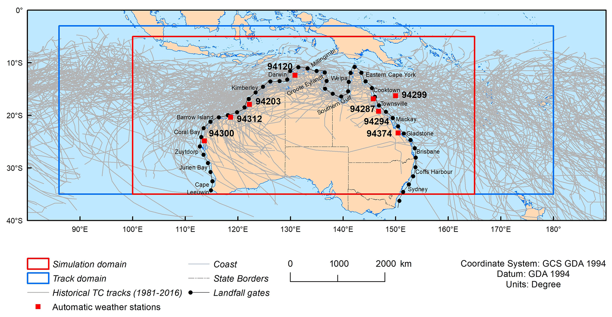
Figure 1Historical TC tracks (1981–2016), simulation domain, track domain, automatic weather stations (with station number) and coastal gates (50 km offshore, 200 km wide) used for landfall analysis (selected gates labelled).
Further, the absolute accuracy of the input data is viewed as a source of uncertainty in the hazard values presented here. For example, Courtney and Burton (2019) reported on progress to improve the best-track archive in Australia, noting the reassessment of intensity due to improved reanalysis methods. Such changes in the intensity values will flow through the hazard model to produce changes in the likelihood of extreme wind speeds. A thorough treatment of the accuracies arising from changes in the best track is warranted (Harper et al., 2008), and the hazard values herein should be considered only one view of the true wind hazard arising from TC events. Yet another aspect that remains to be explored is the effect of centennial and longer variability in TC activity (Haig et al., 2014; Nott et al., 2007).
There are some attributes of TCs that are not reported in the IBTrACS dataset. The radius to maximum wind (Rmax) and pressure of the outermost closed isobar (poci) are two useful values that can provide additional constraints on the intensity and size of TCs. For these variables, we use data obtained from the Joint Typhoon Warning Center (2017), spanning 2002–2016 (15 years). These data are used to develop parametric models for these variables (described in Sect. 3), which are then used in the stochastic track generation process.
It is possible to use data sources other than observational best-track archives as input to TCRM. For example, Siqueira et al. (2014) used tropical-cyclone-like vortices (TCLVs) extracted from global circulation models as a source of track data for evaluating TC wind hazard in the southwest Pacific. After correcting the intensity distribution of the TCLV data, the resulting hazard assessment provided quantitative estimates of the projected change in TC wind hazard.
The TCRM software has been developed at Geoscience Australia as a free, open-source software package. It is written in Python (version 2.7), utilising the Numerical Python “NumPy” (van der Walt et al., 2011), Scientific Python “SciPy” (Oliphant, 2007), netcdf4-python (Unidata, 2018), pandas (McKinney, 2010), Matplotlib (Hunter, 2007) and seaborn (Waskom et al., 2018) packages for statistical and visualisation functions. Additionally, we use some C code for optimisation. The software is available from Geoscience Australia's GitHub repository (Geoscience Australia, 2018), and users can contribute to further development of the model. For this study, we used TCRM version 2.1 (commit reference 8cd4c22 – https://github.com/GeoscienceAustralia/tcrm/releases/tag/v2.1, last access: 12 October 2018), and made use of the National Computational Infrastructure's high-performance computing systems for executing the simulations and analysis of the results.
Simulation times are dependent on the extent of the domain and the number of simulated years. For the domain used in this paper, the data processing and statistical analysis stages take around 15 min to complete on a modern desktop computer. The generation of tracks for a 10 000-year simulation takes around 5 to 6 CPU hours (2.6 GHz clock speed), while the corresponding wind fields (a total of around 160 000 separate events for this simulation) take around 3000 CPU hours. The determination of ARI wind speeds requires a similar amount of CPU time, but the majority is consumed in reading the required data from the wind field files.
TCs in the Australian region often display complex behaviour, with many tracks exhibiting sudden turns (e.g. TC George, 2007) and loops (e.g. TC Hamish, 2009). Despite this behaviour, the translation speed and bearing of TCs still display significant autocorrelation (Figs. 2 and 3), while there is also a moderate autocorrelation in the rate of pressure change across the entire region (Fig. 4).
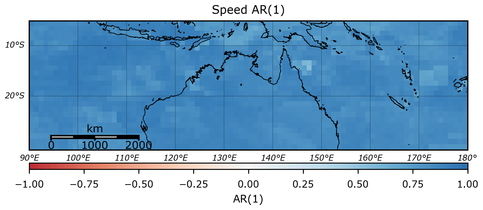
Figure 2Lag-1 autocorrelation of TC translation speed, based on IBTrACS v03r09 (1981–2016). Values are calculated on a 1×1∘ grid.

Figure 3Lag-1 autocorrelation of TC bearing (direction of movement), based on IBTrACS v03r09 (1981–2016).
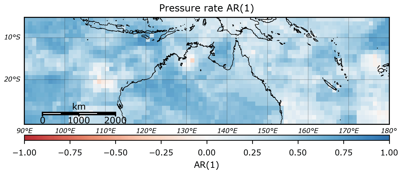
Figure 4Lag-1 autocorrelation of central pressure rate of change, based on IBTrACS v03r09 (1981–2016).
The track model is based on the approach used by Hall and Jewson (2007) and Rumpf et al. (2007), utilising a lag-1 autoregressive technique to model the future behaviour of each synthetic TC. We extend this autoregressive technique and apply it to the intensity (minimum central pressure) of the simulated TCs as well as to the track behaviour.
Users specify a simulation domain, over which the TC wind hazard will be evaluated (Fig. 1). To ensure the simulated events capture the complete range of potential tracks entering this domain, an expanded track domain is defined. The track domain is determined by examining the extent of all historical tracks that enter the simulation domain. The frequency and behaviour of simulated TCs is then determined on the basis of observed events in the track domain.
The model is trained on the observed track data, using a series of 1∘ by 1∘ grid cells across the track domain to capture spatial variability in the descriptive statistics (mean, standard deviation and lag-1 autocorrelation coefficient) for selected TC parameters (speed of forward motion; bearing; intensity; and, where available, Rmax). For each grid cell, a minimum of 100 valid observations are required before descriptive statistics are calculated. If there are insufficient valid observations, then the search area is expanded in steps of 1∘ zonally (east–west) and 0.5∘ meridionally (north–south) – to the maximum extent of the track domain – until sufficient observations are found. Distributions for at-sea and over-land conditions are calculated separately to allow for different behaviours in these circumstances – specifically intensity in near-coastal areas.
Regression models are used to control specific sub-components of the track model – Rmax, poci and landfall decay rate. These regression models are derived from observed data in the Australian region but could equally be adapted to other regions. The code repository provides access to the analysis tools used to determine these regression models and can be used to re-evaluate the regressions for other basins. The model is intended to be applied to regional basins, rather than to a global domain, but the ability to adapt these regression models allows users to run them in basins other than Australia.
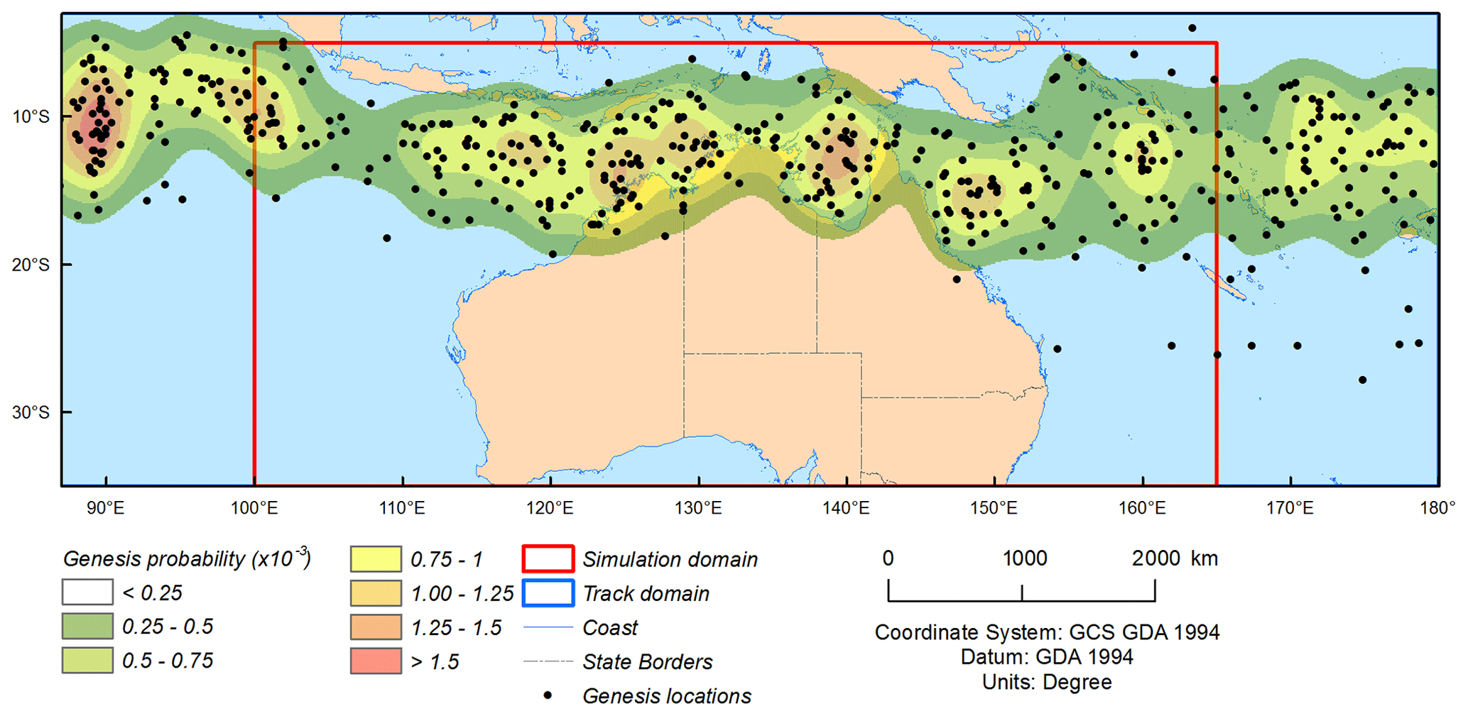
Figure 5TC genesis points for historical TC events (1981–2016) and the corresponding probability density function (TCs per year). Points do not represent the first observation of TC intensity – rather, they represent the first point recorded in the best-track database.
4.1 Genesis
Genesis of TCs is modelled as a Poisson process based on historic frequency in the track domain, with locations of genesis randomly sampled from a two-dimensional probability density function (PDF) of historic genesis points (Fig. 5). The PDF is generated using multivariate kernel density estimation (Silverman, 1986), utilising a two-dimensional Gaussian kernel. The PDF for genesis at a location (λ, ϕ) is
where N is the number of genesis points and di is the distance between genesis point i and the point (λ, ϕ) (latitude and longitude). L is a two-by-two bandwidth matrix determined automatically from the covariance of observed genesis points using a cross-validated maximum-likelihood approach and is held constant over the entire simulation domain. The annual cycle of genesis is included in determining the start time of TC events.
This can result in simulation of genesis over land in the stochastic sampling step. In the Australian region, it is not unusual to observe the formation of precursor tropical lows over land. To allow for this in TCRM, weak lows are maintained if their central pressure deficit increases above 5 hPa within 12 h of the initial time. This allows for initial formation over land (or in areas of positive pressure tendency), as long as the incipient TC intensifies sufficiently (through the stochastic process described in the next section) – usually associated with a move over open water.
The resulting genesis distribution of simulated events does not exactly match the historical distribution for a number of reasons (Fig. 6). Firstly, the stochastic sampling of the distribution for each simulated year will produce a different spatial pattern. In the case of simulating a large number of years, this would intuitively converge to the observed distribution. However, the subsequent track behaviour determines if the track is retained – for example the simulated genesis density may be reduced in regions where tracks are excluded due to rapid weakening or exiting the domain.
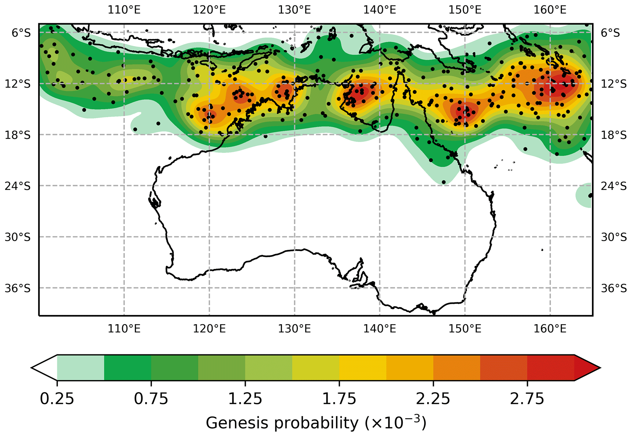
Figure 6TC genesis points and corresponding probability density function for a sample of 35 simulated years of TC activity. Note the different scale compared to Fig. 5.
4.2 Tracks
Following determination of the initial location, intensity, translation speed and bearing of a TC event, the model applies an autoregressive process to step the TC forward in time. Equations (2) and (3) describe the translation speed of the TC located in grid cell i at time t (for the translation speed v):
where is the observed mean translation speed v in grid cell i, is the observed standard deviation of v, is the observed lag-1 autocorrelation, and . controls the magnitude of the random variation ε and is related to through Eq. (4) (noting the change in use for the symbol ϕ from Eq. 1):
ε is a random value sampled from a logistic distribution with zero mean and unit variance. A logistic distribution is used because the heavier tails provide a better representation of the distribution of residuals. Further, comparisons of full track simulations gave qualitatively better results when using the logistic distribution. A corresponding approach is used for the bearing (direction of movement) of simulated TCs.
Intensity, measured as the minimum central pressure p(t), is also modelled in a similar manner, except it is the rate of change in intensity that is predicted at each time step t, rather than the intensity itself as described by Eqs. (5)–(7):
where Δt is the model time step in hours. The statistics for central pressure rates of change ( and ) are normalised to be in units of hPa h−1. and are dimensionless and have the corresponding definitions to those for and . The maximum achievable central pressure of a TC is set to and is a purely statistical bound. However, we note that potential intensity (Holland, 1997) is potentially a more instructive limit, and we are presently working on enhancements that will consider this.
is preferred to the absolute pressure deficit due to the lower lag-1 autocorrelation in the tendency values, making it more akin to a true Markov process than to simulating the absolute pressure deficit. Figure 7 shows the autocorrelation for both and p for a selected grid cell in the Coral Sea. In this case, the lag-1 autocorrelation of is 0.3, compared to that of p which is 0.79. Using absolute values leads to rapid and almost one-way variation (i.e. constant increase or decrease) in the intensity. There remains a strong autocorrelation beyond lag 1 for absolute pressure values but not for pressure tendency values (Fig. 8). Figure 9 shows the time history of central pressure of a small sample of tracks that are generated from a single genesis point (20∘ S, 155∘ E) and the same initial central pressure (995 hPa). One storm weakens rapidly over the first 12 h. The remaining storms take between 30 and 200 h to attain maximum lifetime intensity.
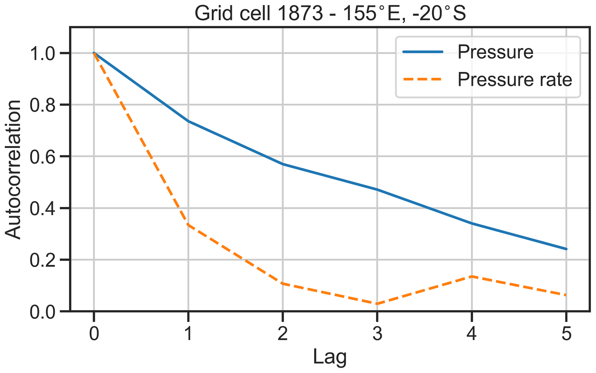
Figure 7Autocorrelation values for minimum central pressure and pressure rate of change, for a single grid cell in the Coral Sea.
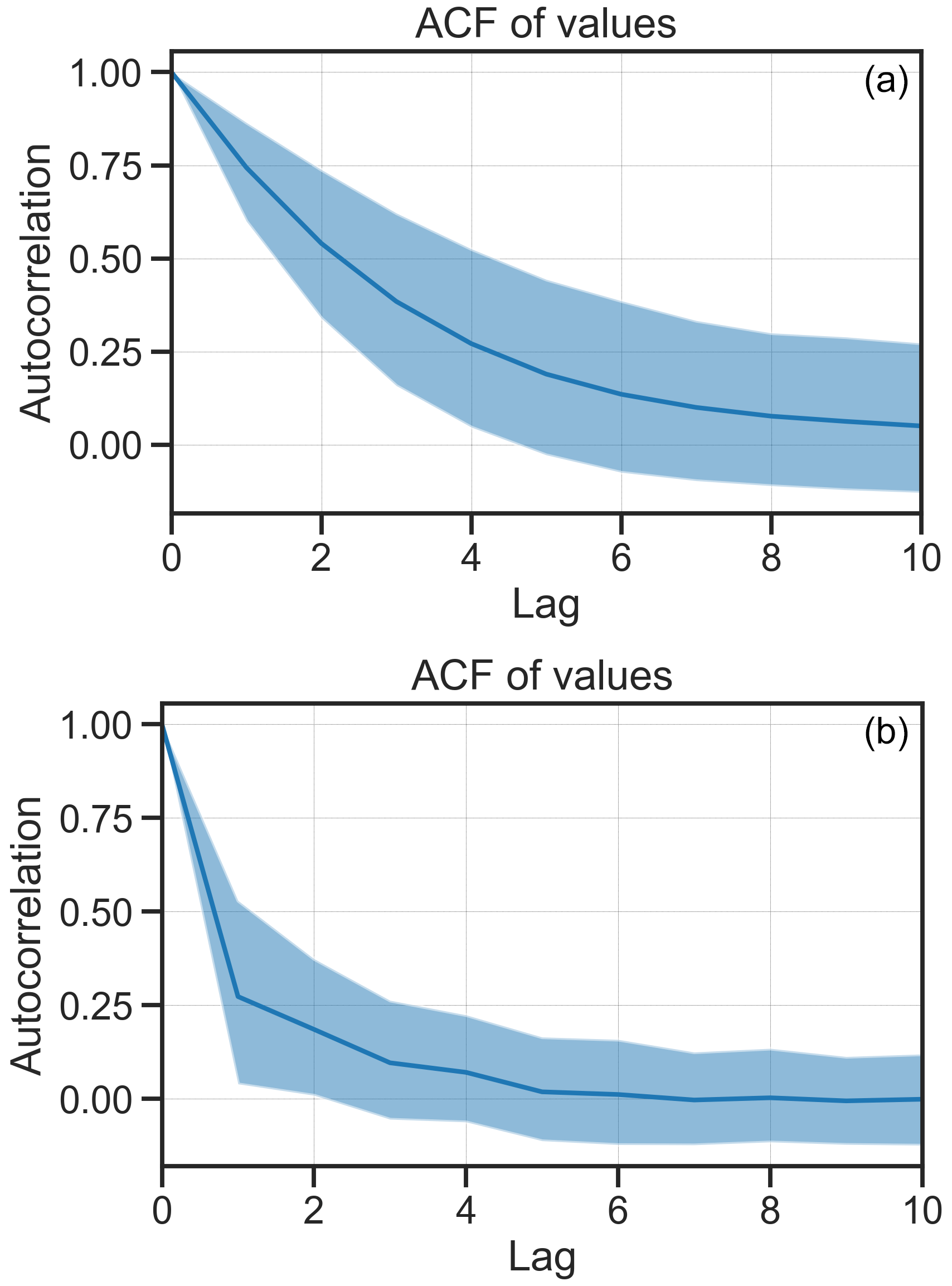
Figure 8Autocorrelation of minimum central pressure (a) and pressure rate of change (b) for lagged observations between 1 and 10 steps. The solid blue line is the mean for all grid cells in the track domain, and the shading is 1 standard deviation.
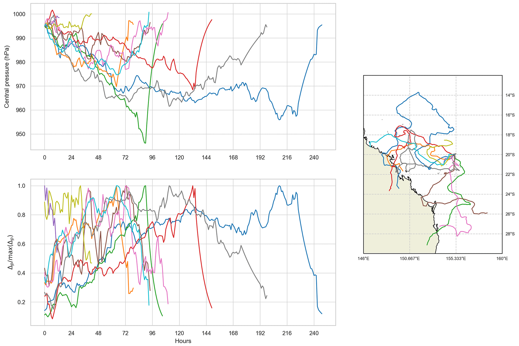
Figure 9Central pressure, normalised intensity, and tracks of 10 events with a common genesis point (20∘ S, 155∘ E) and initial intensity (995 hPa). The lower left panel presents the normalised intensity Δp max(Δp). Colours are for clarity only.
Initial values for , v and storm bearing θ are sampled from the observed distributions of initial values in the initial grid cell, based on the randomly selected genesis point.
4.3 Radius to maximum winds
Where sufficient observed data are available, Rmax is modelled in a similar manner to intensity – i.e. an autoregressive model of the rate of change in Rmax, with statistics calculated from the observed values. In the Southern Hemisphere, Rmax has only been recorded consistently since 2002 by the Joint Typhoon Warning Center (JTWC) (Fig. 10). This means there are generally insufficient data to develop the autoregressive model with confidence across the entire model domain.
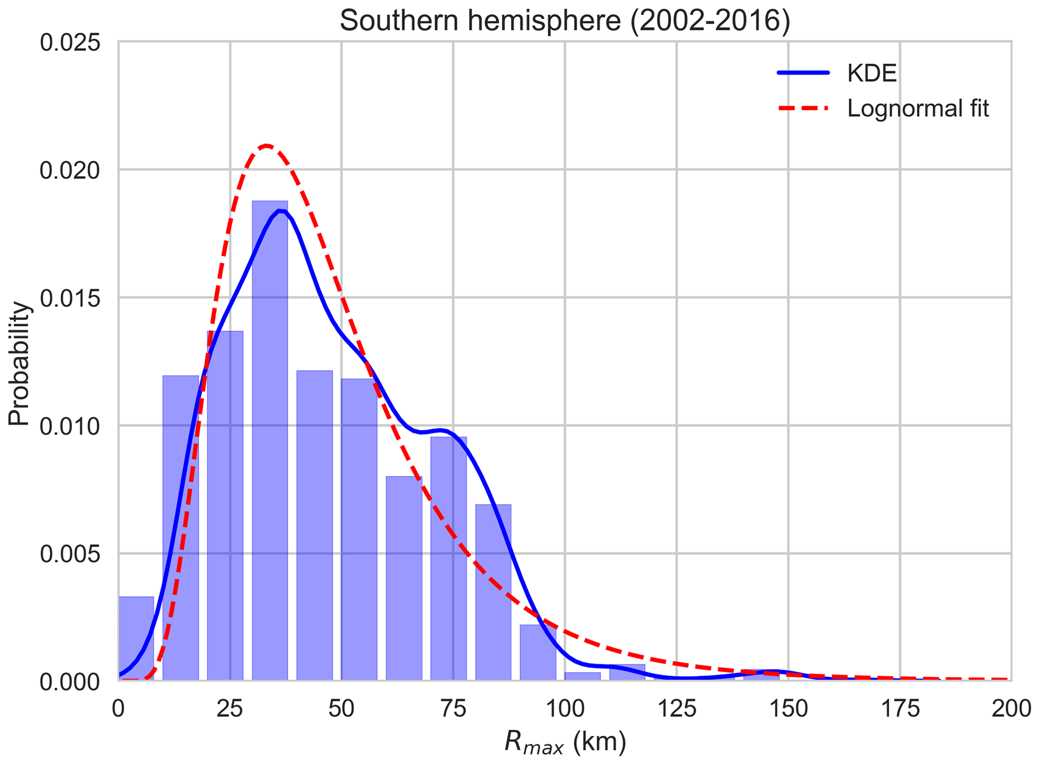
Figure 10Distribution of radius to maximum wind for all Southern Hemisphere TCs (2002–2016). “KDE” is the empirical distribution determined using kernel density estimation; “Lognormal fit” is a fitted lognormal distribution using maximum-likelihood estimation. Data source: JTWC (2017).
In the case of insufficient observations, a parametric model of Rmax is used, based on the model of Powell et al. (2005) and derived using recorded Rmax values from 2002–2016 JTWC records for the South Pacific and south Indian Ocean basins (n=3033):
where Δp is the central pressure deficit (hPa); λ is the latitude (∘); and ε is a random normal variate with mean μ=0 and variance σ=0.335, which is held constant for the life of each individual simulated TC. The functional form is selected to ensure the Rmax values remain bounded at high intensity (large Δp). Coefficients were fitted using non-linear least-squares regression. Figure 11 presents modelled and observed values of Rmax versus Δp, where the modelled values are derived using randomly selected values of Δp and λ. The model slightly overpredicts Rmax at low intensity ( hPa) but otherwise provides an excellent match to the observations.
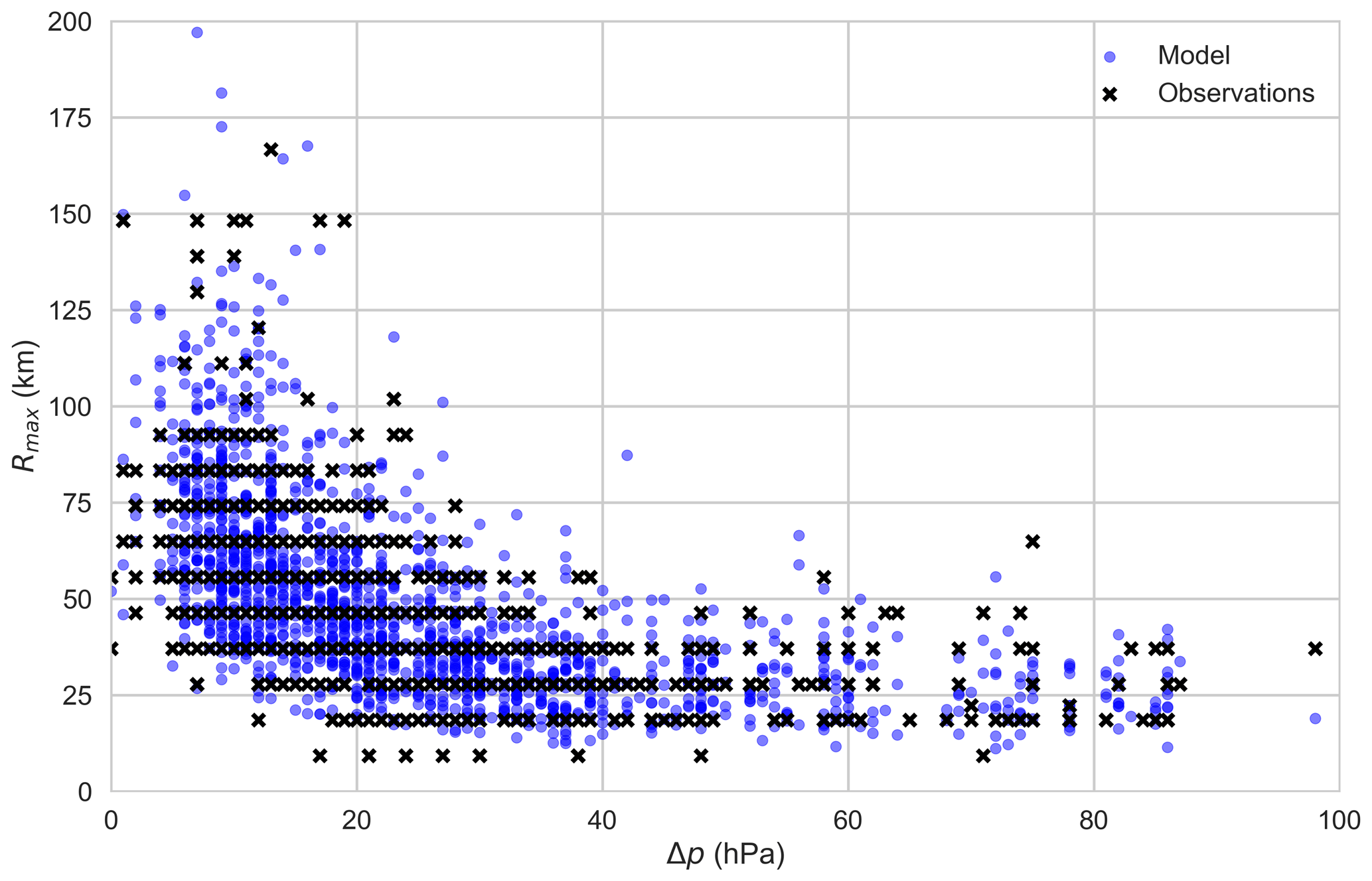
Figure 11Modelled (o) and observed (x) Rmax for Southern Hemisphere TCs (2002–2016), plotted against central pressure deficit. Modelled values are based on a random selection of observed combinations of central pressure deficit and latitude.
4.4 Pressure of outermost closed isobar
The central pressure deficit Δp used to quantify the intensity of synthetic TCs is the difference between the central pressure and the pressure of the outermost closed isobar poci. We initially considered the daily long-term mean sea level pressure at the location of the TC (pltm) as a proxy for poci. However, there are substantial and systematic differences between the two (Fig. 12). Using pltm will lead to synthetic TCs generating sufficient wind speeds to remain defined as TCs at higher central pressure values than observed. To define poci for the synthetic TCs, we modify pltm based on the central pressure, latitude and day of year, plus a random innovation:
where pltm is the daily long-term mean sea level pressure at the location of the TC, pc is the central pressure, λ is the latitude and dyear is the day of year. ε is a random innovation sampled from a normal distribution with μ=0 and σ=2.572. The coefficients were determined using ordinary least-squares fitting to the parameters, using observed values of poci from 2002–2016 JTWC records (n=1833).
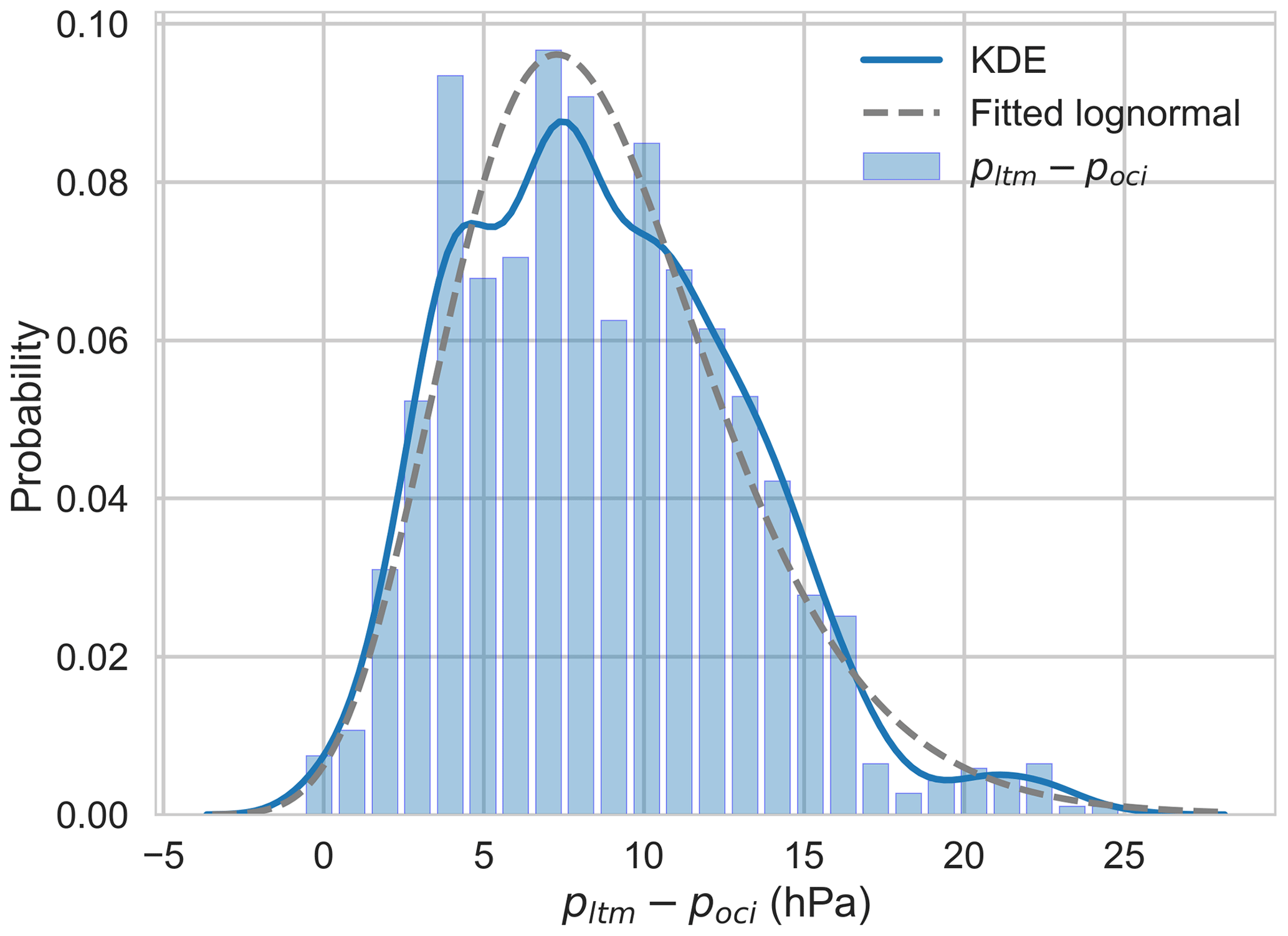
Figure 12Difference between pltm and poci for Southern Hemisphere TCs (2002–2016). Solid line is the empirical distribution determined using kernel density estimation. Dashed line is a fitted lognormal distribution. Data source: JTWC (2016).
Modelled values of poci qualitatively match the observed values (Fig. 13), with l2 norm values all less than 0.4. Closer inspection however reveals subtle differences. When plotted against pltm (Fig. 13a), the maximum density of modelled values of poci is skewed to lower values (approximately 3 hPa lower). For pc versus poci (Fig. 13b), the comparison is much closer, with the peaks in the PDF for both modelled and observed poci coinciding near weak intensity (high pc) and poci near 1006 hPa. Comparison by latitude (Fig. 13c) is very good, with the peak of the PDF of modelled values overlaying the observed peak. The PDF of modelled poci against day of year (Fig. 13d) is also very close to the observed distribution.

Figure 13Observed (shaded) and modelled (contours) distribution of poci for Southern Hemisphere TCs, plotted against (a) pltm, (b) pc, (c) latitude and (d) day of year. Modelled values are based on a random selection of observed combinations of pc, pltm, latitude and day of year. Contour interval is 0.01. Note the different horizontal scale in each panel.
4.5 Landfall
Initial testing using only the autoregressive model for intensity after landfall resulted in unrealistically long-lived tracks after landfall. Instead, the filling rate of TCs after landfall is modelled in the same manner as Vickery (2005), where the central pressure deficit Δp decreases as an exponential function of time over land t, the central pressure deficit at landfall Δp0 and the translation speed at landfall v0:
where
To determine an optimum value for the parameters α0, α1 and α2, the decay behaviour of 174 landfalling TCs recorded in the IBTrACS dataset was analysed (Fig. 14). Δp0 is the last observation of the central pressure deficit prior to landfall, and all observations of Δp after landfall are normalised by this value. Differences in the decay rate of TCs can be identified between those making landfall on the northwest Australian coastline and the eastern coastline (Fig. 15). We hypothesise that this is due to the presence of the Great Dividing Range along the eastern coast of Australia, with elevations exceeding 1400 m in places (e.g. Mt Bartle Frere and Mt Bellenden Ker). Further, the mean central pressure of landfalling cyclones in eastern Australia is higher than those along the western Australian coastline (Fig. 16). In the interest of minimising the data demands (especially with a view to application in other basins), topography was not included in the regression such that we do not have to source suitable topographic data for all potential basins. However this is an area for future development.
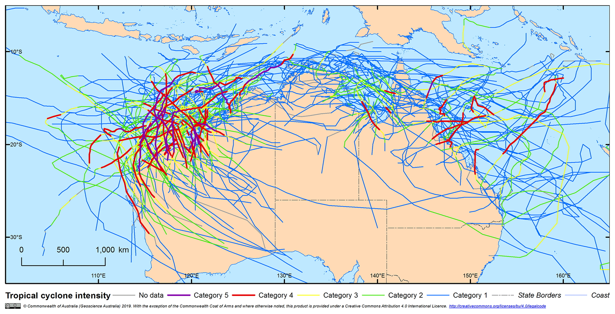
Figure 14Landfalling tropical cyclones in Australia, 1981–2016. Source: IBTrACS v03r09 (1981–2016).
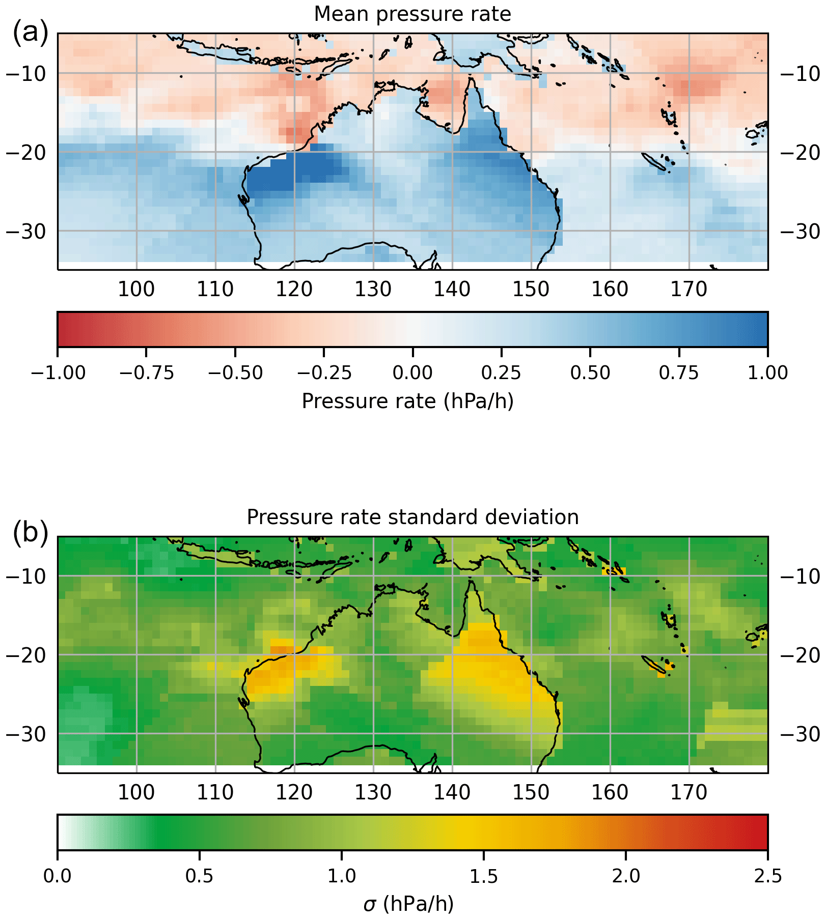
Figure 15Mean (a) and standard deviation (b) of rate of change in central pressure (hPa h−1), based on IBTrACS v03r09 (1981–2016).

Figure 16Mean central pressure (hPa), based on IBTrACS v03r09 (1981–2016).
An exponential decay function was fitted to the normalised pressure deficit for the 174 landfalling TCs (Fig. 17). In general, Δp follows the expected exponential decay form with α defined as
where ε is a random variate sampled from a lognormal distribution with μ=0.6953 and σ=0.0471 and held fixed for each event. Coefficients were fitted using non-linear least-squares optimisation. This gives a decay rate parameter that is influenced by central pressure at landfall and replicates the observed decay rates well (Fig. 18). The effect of the landfall decay model can also be seen in several of the storms in Fig. 9. Storms that move back over open water revert back to the stochastic intensity model, with some storms showing reintensification. For example, track 0 makes landfall after about 220 h and weakens but reverts back to the stochastic intensity model near 235 h, before a second landfall at 242 h.
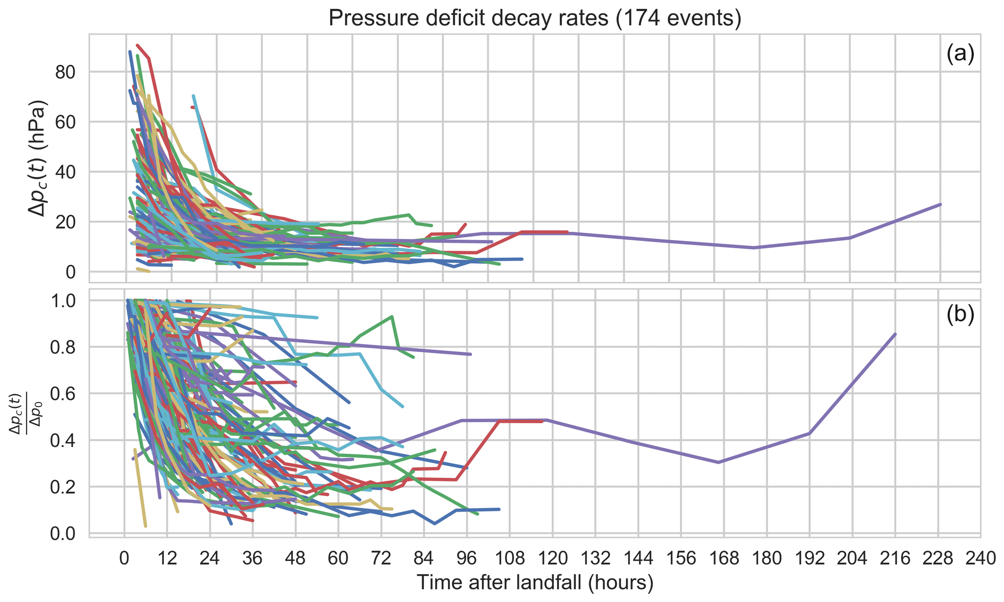
Figure 17Observed pressure deficit versus time after landfall (a) and normalised by pressure deficit at landfall (t=0, b). Colours are for clarity only.
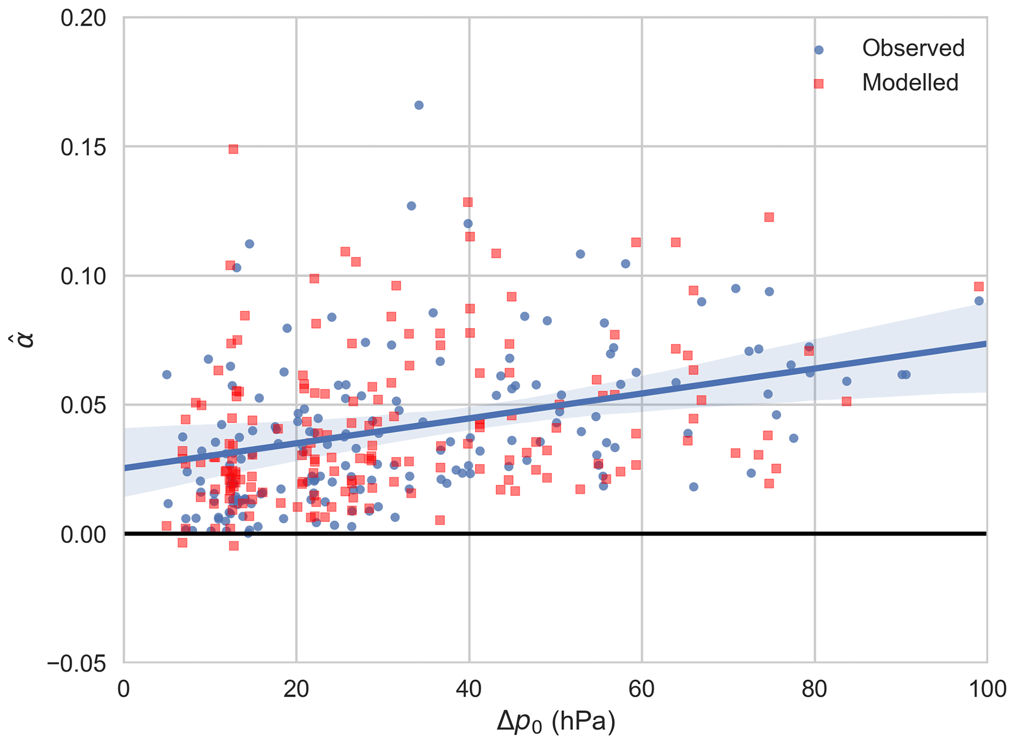
Figure 18Observed and modelled pressure deficit decay rates (α) as a function of landfall pressure deficit (Δp0). The regression line includes the approximate 95 % confidence interval (shaded) based on bootstrap resampling of the observed values. Δp0 values used for the modelled decay rates are randomly sampled from the observed values. See text for details of the model equation.
4.6 Lysis
Lysis of a synthetic TC occurs when Δp falls below an arbitrary threshold, set to be 5 hPa, either due to the decline in intensity following landfall or through the autoregressive process described above. TCs are also terminated on exiting the track domain.
Parametric wind fields are calculated for each event in the synthetic catalogue to enable a high-spatial-resolution understanding of the ARI wind speeds. The additional benefit of this calculation is that users can select individual synthetic events from the catalogue and obtain a wind field for use in scenario simulations.
5.1 Radial wind profile
The wind field around each TC is calculated at high spatial resolution (up to 0.01∘) to ensure the peak wind speeds near the eye are accurately captured. TCRM first uses a radial profile to estimate the gradient level wind associated with the vortex. To allow users to explore the range of variability in ARI wind speeds associated with different radial profiles, we have implemented a number of profiles in TCRM. These include the Holland (1980), Schloemer (1954), Willoughby and Rahn (2004), Powell et al. (2005), and Jelesnianski (1966) profiles; the McConochie et al. (2004) double exponential profile; and a Rankine vortex profile. The Willoughby, Schloemer and Powell et al. profiles are all variants of the Holland profile – the difference being the definition of the peakedness or β parameter. While more complex radial profiles are available in the literature, we have chosen to implement simpler models that rely only on readily available best-track parameters (e.g. central pressure, latitude). For this verification study, the Powell et al. (2005) profile was used, with β defined as
where λ is the latitude of the TC centre and ε is a random variate sampled from a normal distribution with zero mean and a standard deviation of 0.286. The random innovation term is held fixed for each storm event.
5.2 Boundary layer model
In addition to the range of radial profiles, users can also select one of three boundary layer models. These boundary layer models relate the winds at the gradient level to those near the surface, taking into account the asymmetry induced by the forward motion of the TC and surface friction effects. In parametric TC models, this is often achieved by vector addition of the forward motion and the gradient winds together with a surface wind reduction factor. Examples of this type include the McConochie et al. (2004) model, which varies the inflow angle as a function of radial distance, or the Hubbert model (Hubbert et al., 1991). Alternatively, a linear analytic model (Kepert, 2001) of the boundary layer flow can be applied with minimal computational cost.
In this study, the linear boundary layer model of Kepert (2001) was applied to relate gradient level winds to surface winds. This model utilises a bulk formulation for the boundary layer with the drag coefficient set to a constant value of 0.002 and the turbulent diffusivity for momentum set to 50 m2 s−1, as recommended by Kepert (2001). The model assumes Vtangential≫Vtranslation, which may be violated for low-intensity storms (e.g. incipient TCs). The boundary layer model is modified to linearly reduce the effects of translation speed when Vtranslation>0.2Vtangential. The effects are also reduced to zero at distances greater than 2Rmax, using an inverse-square decay function.
The linear analytic model generates a surface wind speed corresponding to a 1 min mean wind speed (Khare et al., 2009). This is converted to a 0.2 s gust wind speed using a wind speed conversion factor determined using the approach outlined in Harper et al. (2010). The resulting wind fields represent a 10 m above ground, 0.2 s gust wind speed over flat terrain with an aerodynamic roughness length of 0.02 m. This is carried across the entire simulation domain, including over-water areas. This choice is made to enable direct comparison to other measures of regional-scale wind hazard such as weather station observations. For more localised wind speeds that can be used for detailed wind impact calculations (e.g. Krause and Arthur, 2018), local site conditions can be incorporated via an offline calculation that can incorporate local accelerations over topography and varying surface roughness conditions (Yang et al., 2014).
Throughout the simulations, it is assumed the gradient level wind is axisymmetric. However, the simulated tracks can extend to mid-latitudes, where TCs undergo transition to extra-tropical cyclones and the gradient level wind becomes asymmetric (Foley and Hanstrum, 1994; Jones et al., 2003; Loridan et al., 2013). Further, the assumption in the linear boundary layer model that Vtangential≫Vtranslation does not hold for transitioning storms, where Vtranslation can exceed 70 km h−1 (Foley and Hanstrum, 1994). This means the simulated hazard values in the mid-latitudes (approximately poleward of 30∘ in the southeastern Indian Ocean) are likely not indicative of the true wind hazard associated with (transitioning) TCs. It is also likely in these regions that other phenomena (e.g. thunderstorms) are the predominant source of extreme wind gusts. There are promising developments in the area of extra-tropical transition (Loridan et al., 2015; Bieli et al., 2019), which have direct application in probabilistic modelling frameworks and may be integrated into TCRM in future releases.
Once wind swaths for the simulated TCs have been generated using the wind field module, the maximum wind speed from all simulated events, irrespective of direction, for each grid point is stored. Because of the large number of events simulated, it is possible to estimate average recurrence intervals (ARIs) for the wind speeds at each grid point. The simplest approach is to use an empirical approach based on Eq. (14):
where ri is the wind speed rank of the ith event, nobs=365.25 is the number of values per simulated year and is the total number of simulated “daily” observations for the 10 000-year simulation. For each point across the simulation domain, we treat each simulated event as an individual daily observation and rank the simulated wind speeds from all events. This usually produces around 105 records (depending on the frequency of TCs at that location). The remaining daily records are zero filled.
A more sophisticated approach is also implemented, where the simulated maximum wind speed values are fitted to a generalised Pareto distribution (GPD) using a peaks-over-threshold approach. ARI wind speeds are estimated from the GPD parameters using Eq. (15):
where w is the wind speed with an ARI of t years. μ, σ and ξ are the location, scale and shape parameters of the fitted GPD distribution respectively, and ρ is the rate of exceedances above the threshold u. The threshold is set to the 99.5th percentile of the simulated wind speed values. As wind speeds are considered a bounded phenomenon (Lechner et al., 1992), the fitted shape parameter ξ can be constrained to be positive to ensure the resulting distribution is bounded at long return periods (Holmes and Moriarty, 1999). Again, this parameter fitting is performed at each point across the region of interest, leading to a spatial representation of ARI wind speeds.
Confidence intervals are estimated from the covariance matrix of the parameter fit. This method is useful for estimating winds speeds at very long ARIs, where the frequency of events is very low. ARI wind speeds estimated using this method tend to be underestimated at lower ARIs compared to the empirical approach, largely because the threshold selection excludes lower, more frequent wind speeds.
7.1 Track model verification
To evaluate the performance of the model, we run a series of comparisons between the observed tracks and a large number of simulated track sets. A total of 1000 synthetic-event sets were generated, each representing 35 years of TC activity, mimicking the length of the input historical record. For each metric, historical values are compared to the mean value for the collection of synthetic-event sets, with 90th-percentile confidence intervals calculated using bootstrapping methods.
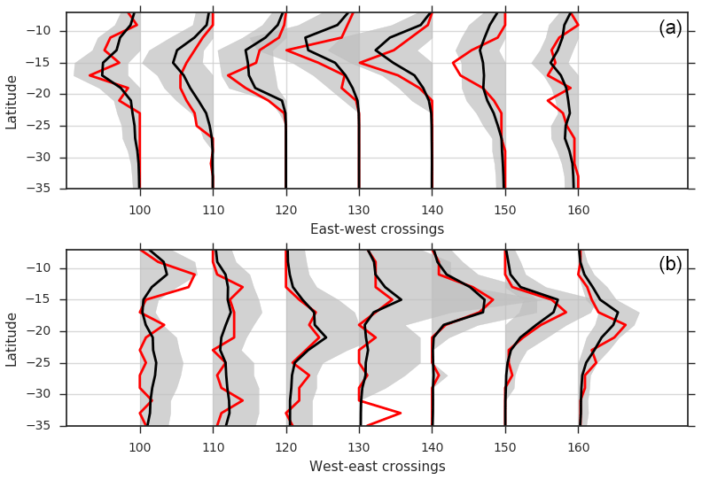
Figure 19Distribution of longitude crossing rates for synthetic and observed TCs. Values represent 100 times the probability density of events crossing each longitude in 2∘ latitudinal segments. (a) TCs moving east to west; (b) TCs moving west to east. Red lines are the observed distribution (IBTrACS v03r09 1981–2016); black lines are the mean of 1000 simulations each representing 30 years of activity. Shaded band indicates the 90th-percentile range of the simulations.
The distribution of observed longitude crossing rates is well modelled for both eastward- and westward-moving storms (Fig. 19). The values represent the probability density of events crossing each longitude in 2∘ latitudinal segments. In general, the model simulates the longitude crossing rates well. Near 15∘ S, 150∘ E, the model does not capture the rate of TCs crossing the Cape York Peninsula, which is related to the termination of TCs due to low intensity. Similar overall results are obtained for longitude crossing rates when the model is tested in the western North Pacific and Atlantic basins (not shown), including in middle to high latitudes, capturing the paths of recurving TCs.
TCRM simulations of minimum central pressure perform well, especially for the more intense (lower minimum central pressure) TC events (Fig. 20). The lower tail of the simulated distribution closely follows the observed tail. For weak TC events (>980 hPa), the observed distributions lie outside the 90th percentile of the simulations. This has little impact on the derived extreme wind speeds, which are generated by the most intense TCs.
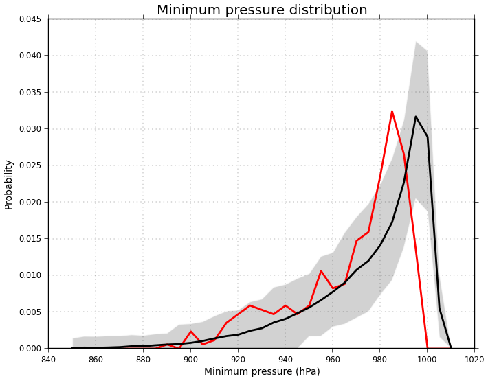
Figure 20Distribution of minimum central pressure values (hPa). Red line is the observed distribution (IBTrACS v03r09 1981–2016); black line is the mean of 1000 simulations each representing 35 years of activity. Shaded band indicates the 90th-percentile range of the simulations.
The spatial distribution of minimum central pressure is presented in Fig. 21. Values represent the lowest minimum central pressure value observed in each 1∘ by 1∘ grid cell in the historical record. We apply the same process to each 1000 synthetic-event set, and the mean of those is presented. There is general agreement between the synthetic and observed (historic) distributions, though individual events in the historic record do result in greater variability. The spatial distribution of the mean central pressure (Fig. 22), calculated in a similar manner to the minimum central pressure, again shows good agreement between the synthetic and observed event sets, without the large variability seen in the historic minima.
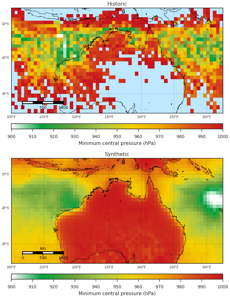
Figure 21Historic and synthetic minimum central pressure values over the simulation domain. Synthetic values are the mean of 1000 simulations of 35 years of TC activity.

Figure 22Historic (a) and synthetic (b) mean central pressure values across the simulation domain. Synthetic values are the mean of 1000 simulations of 35 years of TC activity.
Lifetime maximum intensity (LMI), defined as the maximum wind speed for the life of the TC, can be used to evaluate how well the model simulates the evolution of intensity of TCs. Figure 23 shows the mean location of LMI in the observed (top) and simulated (bottom) records. There is little discernible pattern in the location of LMI for observed TCs. This may in part be due to the small numbers of events available for the analysis (n=377), as only those events with a maximum wind speed recorded were used. The mean LMI is generally evenly distributed throughout the domain, though lower LMI values can be seen over Cape York (145∘ E) and south of Indonesia at low latitudes. For the simulated events, there is a clear trend towards higher LMI at higher latitudes in the Indian Ocean, with the highest LMI simulated at 20–25∘ S. There are also indications that LMI increases towards the south in the Coral Sea to the east of Australia.
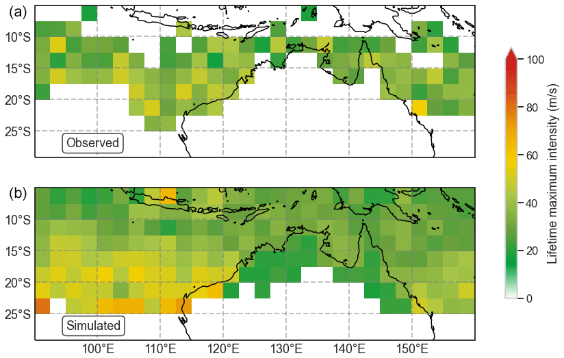
Figure 23Historic (a) and synthetic (b) mean lifetime maximum intensity. Synthetic values are the mean of 1000 simulations of 35 years of TC activity.
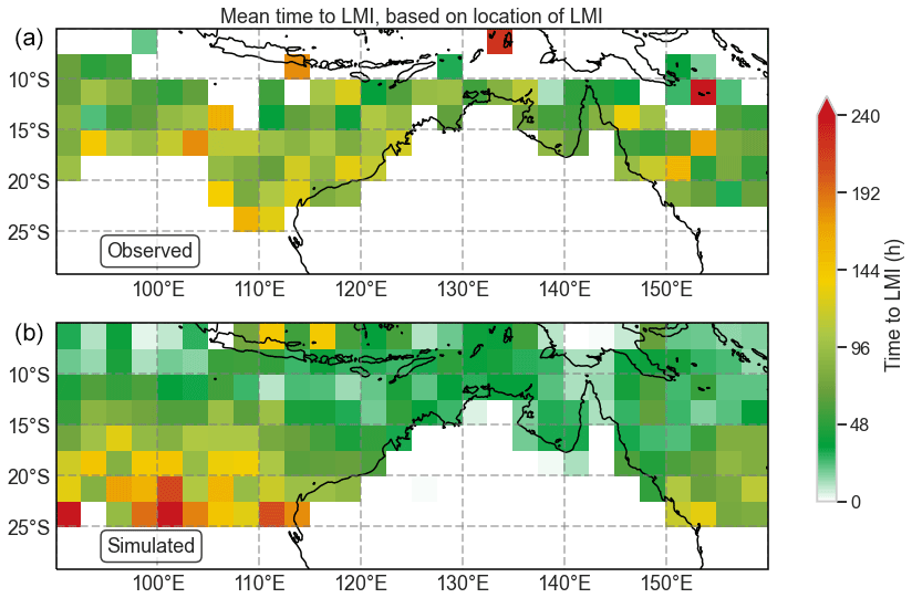
Figure 24Mean time taken (h) to achieve lifetime maximum intensity for historical (a) and synthetic (b) TCs. Synthetic values are the mean of 1000 simulations of 35 years of TC activity.
The average time taken to achieve LMI for observed TCs (Fig. 24, top) shows little clear pattern, though the areas off the western coast of Australia do tend to be slightly higher. The simulated tracks (bottom) display a strong tendency to achieve LMI at higher latitudes (>17.5∘ S) and take longer to achieve LMI in these areas. This may lead to higher ARI wind speeds at these higher latitudes. Comparing geographical areas, the observed time to reach LMI off the northwest coastline is around 96–144 h, while the mean time to reach LMI is only around 48–72 h for simulated events. On the east coast, there appears to be less difference between observed and simulated time to reach LMI, but there are a greater range of values, ranging between 48 and 120 h.
Figure 25 presents the landfall probabilities around the Australian coastline. Each gate is 200 km wide and located approximately 50 km off the coast (Fig. 1). TCRM replicates the observed probability of landfall well, with the mean of the synthetic-event sets generally close to the observed probability. The relatively low occurrence of landfall around the Australian coastline (on average only four TCs cross the coast each year) means there is large variability in the landfall count for any given synthetic-event set. Again, qualitatively similar results are obtained for simulations in the western North Pacific and Atlantic basins (not shown).
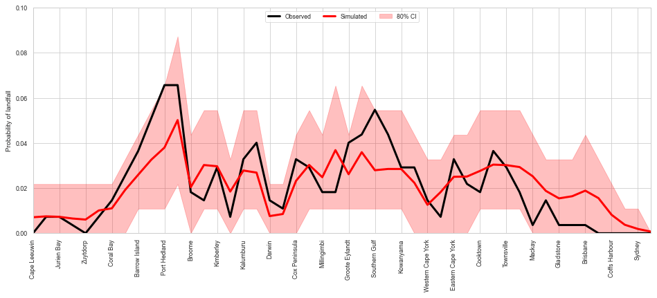
Figure 25Probability of a TC making landfall around the Australian coastline. Black line is the observed distribution (IBTrACS v03r09 1981–2016); red line is the mean of 1000 simulations each representing 35 years of activity. Shaded band indicates the 80th-percentile range of the simulations.
At all times the 80th-percentile range captures the observed landfall probability, as expected. However, the mean landfall probability in the simulations for the region between Coral Bay and Port Hedland is substantially lower than the observed landfall probability. This is possibly linked to lower genesis probabilities directly to the north of this area. Historically, there is a local maximum in genesis probability between 120 and 130∘ E, extending westward into the Indian Ocean near 10∘ S (Fig. 5). The mean genesis density for the simulations does not show the same local maximum or the westward extension. This lower genesis density is likely translating into lower track densities in the region and therefore lowers landfall rates along the northwest Australian coast. This in turn acts to reduce ARI wind speeds along this part of the coastline compared to observed ARI wind speeds.
When examining the distribution of intensity at landfall (Fig. 26), the proportion of category-5 landfalls along the lower west coast is high, representing around 25 % of landfalls through gates between Cape Leeuwin and Coral Bay. This is hypothesised to be linked to the poor representation of transitioning TCs in this region. The region from Coral Bay to Port Hedland (noted previously for a low landfall probability) displays a similar landfall intensity distribution to observations, where the majority of landfalling TCs are severe (category 3–5). Along the east coast, between Mackay and Coffs Harbour, the proportion of category-5 landfalls is also high (around 20 %). Additionally, the probability of any landfall in this region is significantly higher than for the observations. These two factors contribute to an overestimate of the ARI wind speeds in southern Queensland and northern New South Wales.
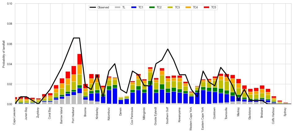
Figure 26Mean distribution of landfall intensity (by TC intensity category) for synthetic TCs. Categories are based on the Australian TC intensity scale. The observed landfall probability is shown in black.
7.2 Wind field model verification
To demonstrate the reliability of the wind field model, we modelled a number of historical TC events using the parametric wind field and compared to observed wind speeds recorded at Bureau of Meteorology weather stations near to the track of the TC. We select stations that are within 100 km of the track, in an effort to verify the modelled events against the strongest winds of the TC and provide a meaningful result. In total, 29 stations and 14 TCs are examined, providing a cursory analysis of the wind field model performance.
The configuration is kept consistent with that used to derive the ARI wind speeds, so no calibration of the parameters (e.g. peakedness parameter) is performed for individual TCs used in the verification (cf. McConochie et al., 2004). We chose not to calibrate for each individual event so as to quantify the capability of the wind field model to reproduce gross features of observed TCs. In a stochastic model such as TCRM, it is important that the wind field model displays no significant bias in wind speed and errors in the mean wind field are minimised. By using a consistent configuration for verifying the wind field model, it is possible to quantify the bias in the wind field that might arise from applying that configuration to a set of synthetically generated TCs. This will generally result in a poorer simulation of each individual TC when assessed using metrics such as root mean square error, since the parameters have not been optimised for the evolution of each individual event. The reader is directed to the references for the profiles and boundary layer model for more thorough validation of those models.
Simulated wind speeds are matched to corresponding observations from weather stations based on the time of observation. The wind field model provides data at 5 min intervals, so it is possible that absolute peak observed values may not match the time interval. Observed wind speeds are corrected for gust averaging time periods (Harper et al., 2010), as the default configuration for TCRM is to produce wind speeds representing a 0.2 s gust wind speed. No corrections for site exposure (e.g. topographic enhancement, surface roughness changes) are made.
Weather station wind histories
For each simulated event, time histories of wind speed and direction at all weather stations within the modelled domain are recorded. Figures 27–30 present the time history for four stations (Mardie, Carnarvon, Lucinda Point and Flinders Reef) during the passage of four separate TCs (Glenda, Olwyn, Yasi and Larry respectively). For each of these events, the TCRM wind field simulation captures the increase in wind speed as the TC approaches the station, with the time of peak wind speeds accurately modelled.

Figure 27Modelled and observed wind speed (a) and direction (b) at Mardie (Western Australia) for the passage of TC Glenda (2006).

Figure 28Modelled and observed wind speed (a) and direction (b) for Carnarvon (Western Australia) for the passage of TC Olwyn (2015).
Changes in wind direction follow the observations closely, except for Lucinda Point (Fig. 29) where the observed winds quickly returned to a southerly direction after the passage of TC Yasi. The simulation shows winds turning anti-clockwise as the TC passes at around 00:00 Z on 3 February 2011, consistent with a cyclonic vortex passing north of the observation site. It appears a similar shift occurs in the observations several hours earlier, but winds turn back to the south rapidly at around 18:00 Z on 2 February. This difference is likely due to the model not containing any other sources of pressure gradient winds from synoptic-scale weather patterns such as high-pressure ridging into the Coral Sea following the passage of the TC (for example, see the discussion in McConochie et al., 1999).
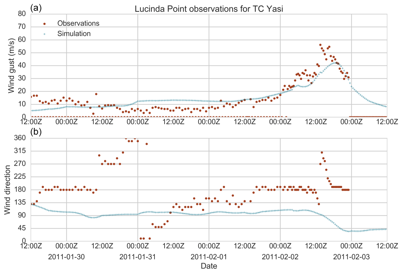
Figure 29Modelled and observed wind speed (a) and direction (b) at Lucinda Point (Queensland) for the passage of TC Yasi (2011).
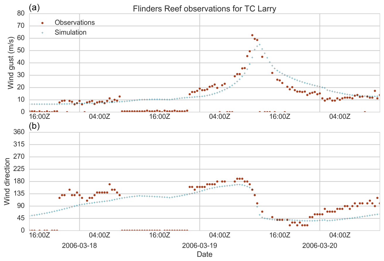
Figure 30Modelled and observed wind speed (a) and direction (b) for Flinders Reef (Queensland) for the passage of TC Larry (2006).
Peak wind speeds are closely simulated, except for Lucinda Point in TC Yasi, where the wind field model underestimates the peak wind speed by nearly 20 m s−1. Among other events (Fig. 29, lower right panel), the tendency is for the TCRM wind field simulation to overestimate peak wind speeds. There are likely several factors (for example, instrument failure or site exposure) leading to this overestimation, which may be drawn out in a more thorough validation of the wind field model and analysis of those events. The results here are likely due to our decision not to correct the observed wind speeds for site exposure, which would reduce the modelled wind speeds.
For the complete time histories (all corresponding time records, not just the peak), Fig. 31 presents the root mean square error, bias and mean absolute error for all 29 stations and 14 events modelled. The average RMSE is 9.2 m s−1 and the bias 1.2 m s−1. In the context of a stochastic model where many thousands of events will be simulated, the average RMSE outcome is acceptable, but the tendency for peak wind speeds to be overestimated requires further investigation.
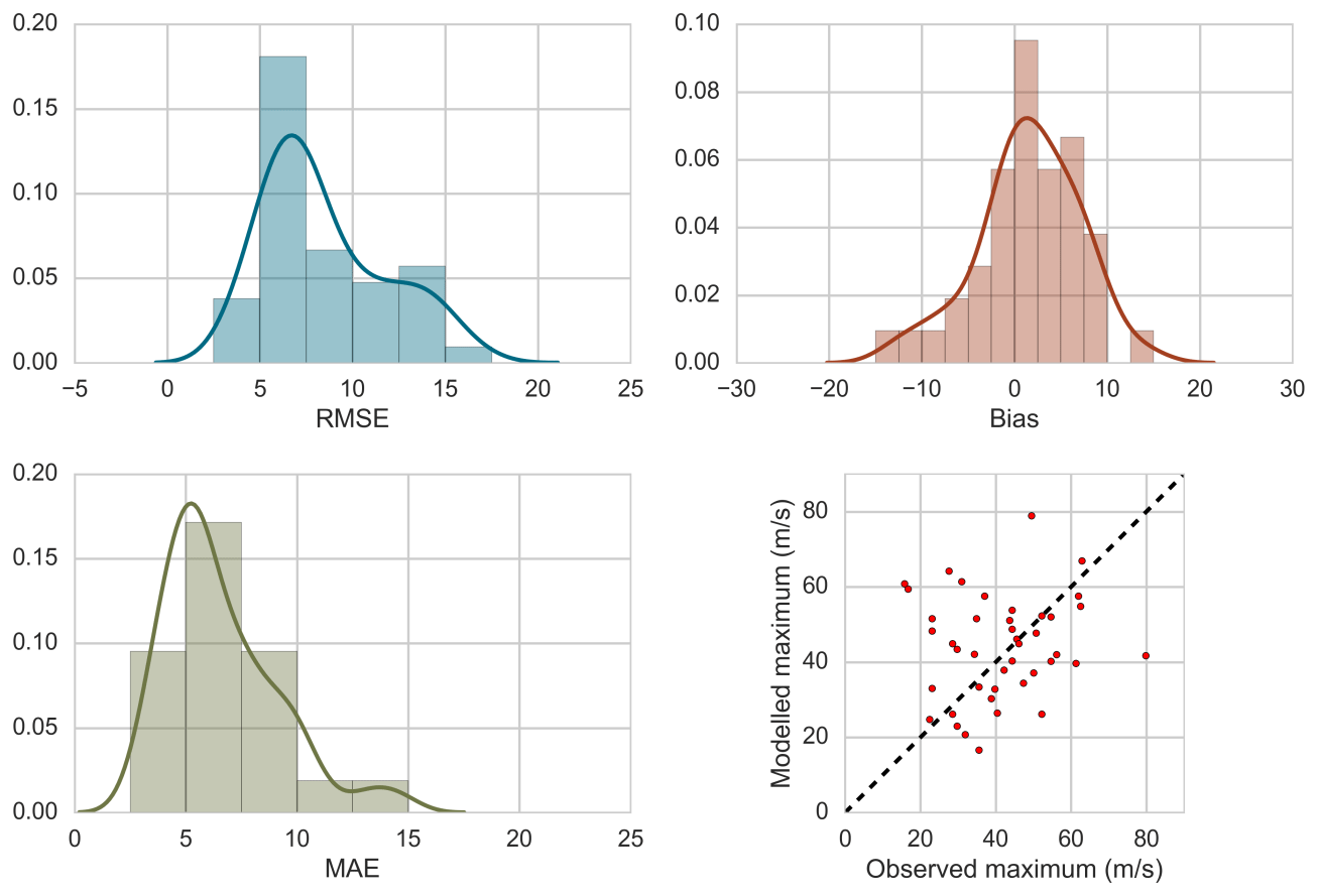
Figure 31Root mean square error (RMSE), bias (Bias), mean absolute error (MAE) and scatter plot of observed versus modelled maximum wind speed for 42 weather station observations associated with the passage of a TC.
7.3 ARI wind speed verification
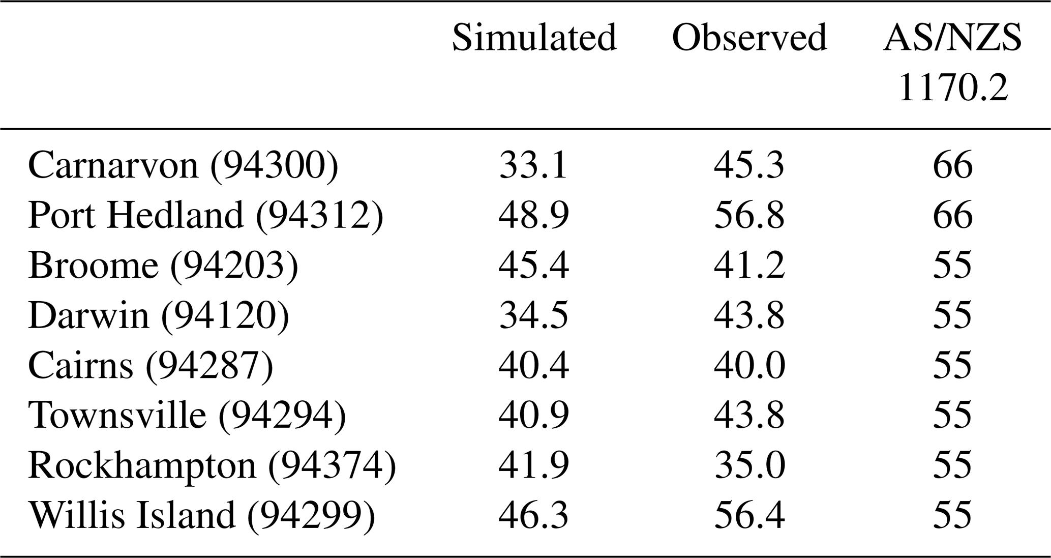
ARI wind speeds for the Australian region are calculated from a simulation of 10 000 simulated TC seasons, or over 160 000 individual simulated TC events. Two ARI wind speeds are examined – the 50-year ARI wind speeds are compared to observed TC-related wind speeds, while the 500-year ARI wind speed is compared to the regional design wind speeds detailed in AS/NZS 1170.2 (2011). We use the 500-year ARI wind speed for comparison, as it represents the regional design wind speed for residential housing in AS/NZS 1170.2 (2011).
Table 1Observed and simulated 50-year ARI wind speeds for selected locations. Simulated ARI wind speeds are taken to be the empirical ARIs. All values are in m s−1.
Observed ARI wind speeds were estimated from daily maximum gust wind speed observations that may be attributable to the passage of a TC, recorded at Bureau of Meteorology weather stations (Fig. 1). All TCs passing within 200 km of the station, when the station was open, were recorded. Daily maximum wind gusts corresponding to the closest passage of each TC were then extracted and empirical ARI values determined based on Eq. (14). Corrections are made for gust wind speed averaging times where instrumentation is known (Harper et al., 2010).
The 500-year ARI wind speed map (Fig. 32) displays qualitative similarities to existing design wind-loading standards (see Fig. 3.1A in AS/NZS 1170.2), at least over continental Australia (the design standard does not define wind speeds over the ocean). The highest wind speeds are estimated along the northwest coast of Australia, with a peak value near 70 m s−1 near Port Hedland (near 120∘ E) for the 500-year ARI. The remainder of the northern and much of the eastern coastline indicates lower wind speeds, generally between 50 and 60 m s−1. The wind speeds drop below 45 m s−1 across Cape York (142∘ E), where there is also a marked decrease in TC frequency. The highest values of 500-year ARI wind speed along the east coast occur around the Rockhampton region, reaching 60 m s−1. ARI wind speeds steadily decline further south, reaching around 50 m s−1 in northern New South Wales. The comparatively high values at higher latitudes (cf. AS/NSZ 1170.2) are likely indicative of the model failing to correctly simulate the extra-tropical transition process noted in Sect. 5.2.
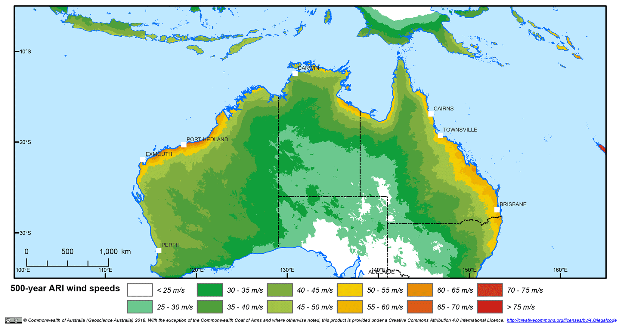
Figure 32The 500-year ARI wind speed due to tropical cyclones across Australia, using empirically estimated return period wind speeds (Eq. 11).
ARI curves for selected locations are presented in Fig. 33, along with estimated ARI wind speeds for observed TC-related wind speeds (see below) at those locations. The solid line is a GPD fitted to the simulated wind speeds using peaks over threshold with a 99.5th-percentile threshold, but here we have relaxed the constraint of ξ>0. The 90th-percentile confidence intervals are determined from the covariance matrix of the fitting routine.
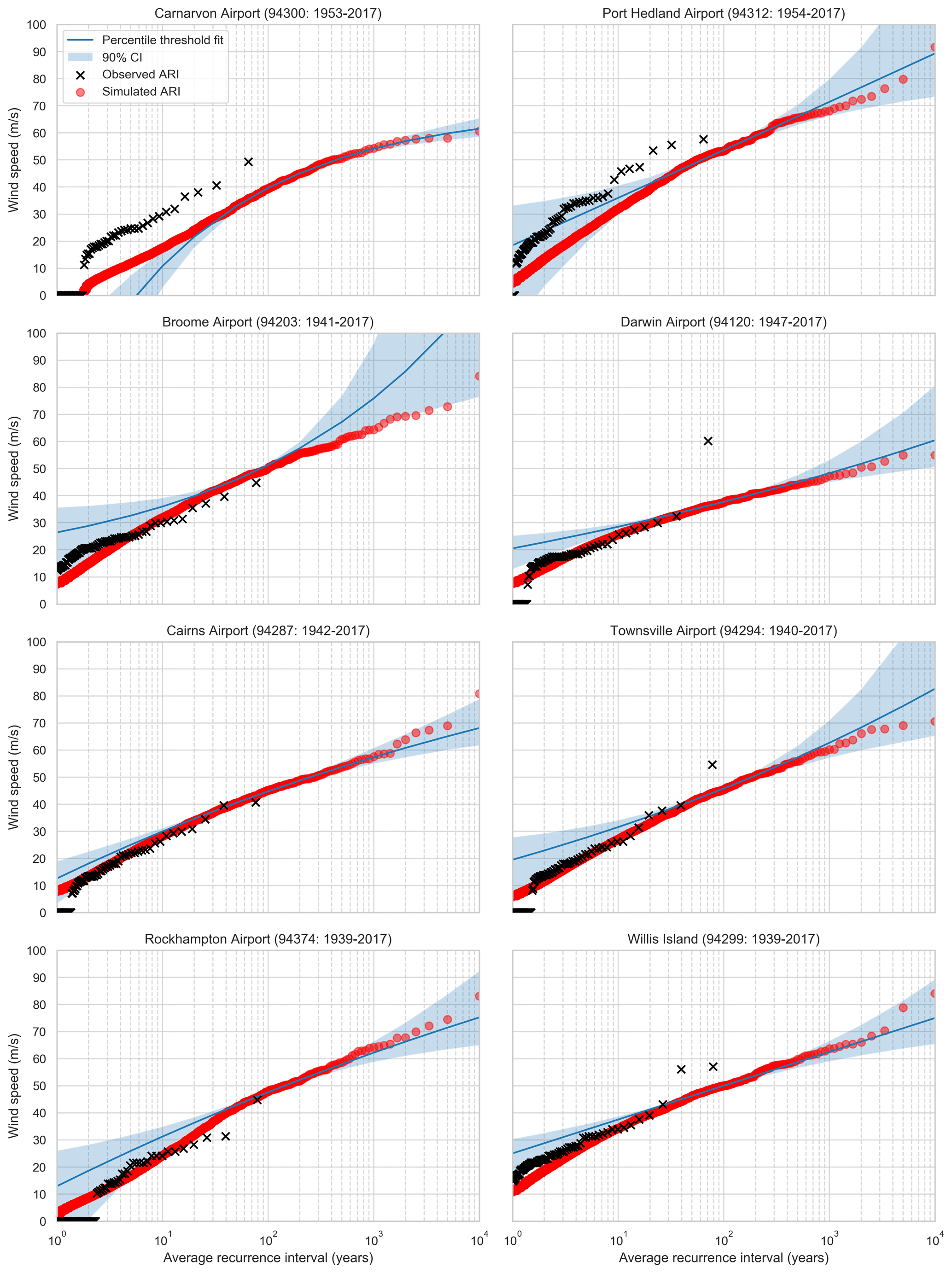
Figure 33Hazard profile for locations around Australia. Estimated ARI wind speeds derived from observed TC wind speeds are marked by “×”. “Percentile threshold fit” (blue line) uses the 99.5th percentile as the threshold for the peaks over threshold for fitting the GPD to the simulated wind speeds from the stochastic-event set (red circles). The blue shading is the 90th-percentile confidence interval of the GPD fit. The title for each panel includes the years of available observational data for the location.
For locations along the west coast (Carnarvon, Port Hedland), the model underestimates the hazard profile compared to the observed hazard profile. For Port Hedland (64 years of records), the simulated 50-year ARI wind speed is just under 50 m s−1, while the observed 50-year ARI is approximately 57 m s−1 (Table 1). Similarly at Carnarvon (65 years of records), the simulated 50-year ARI is 35 m s−1 and the observed 50-year ARI is close to 45 m s−1. This is a significant discrepancy between the simulation and observations. In part, this is attributed to the comparatively low landfall rates along this section of the coastline (Figs. 25 and 26) and so points to additional work on improving the simulation of intense TCs along this section of the Australian coastline, in terms of both event rates and intensity.
In other parts of the country, model performance is much better. Simulated ARI wind speeds at Darwin closely match the observed ARI wind speeds, but the outlying observation of TC Tracy (1974 – 67 m s−1) is cause for further investigation. This analysis places the observed wind speed of Tracy at around a 5000-year ARI, but there is significant uncertainty regarding this estimate and conjecture about the most appropriate way to estimate this from observations (Harper et al., 2012). For east coast locations, the simulated ARI wind speeds for Cairns, Townsville and Rockhampton are all close to the observed ARI wind speeds, varying at the 50-year ARI by at most a few percent. The observed ARI wind speeds generally fall within the 95th-percentile confidence interval of a GPD fitted to the simulated values (not shown). It is also notable that observed and simulated ARI wind speeds lie below the corresponding regional wind-loading design levels specified in AS/NZS 1170.2 (2011) for all locations, except for Port Hedland where observed ARI wind speeds are close to the regional design level.
An important component of stochastic models is to check for convergence in solutions (Shome et al., 2018). For TCRM, this can be checked by splitting the synthetic catalogue into two subsets, calculating ARI values from each and examining the range of values. A large difference in ARI wind speeds indicates the model has not converged. It is expected that at large ARIs the model would not converge, as variability in the tail of the distribution is to be expected when modelling rare events. Significant difference in the ARI values for the two subsamples indicates the variability in the distribution is large. Figure 34 shows the convergence checks for the locations mentioned above. Carnarvon, Port Hedland and Willis Island show little difference in the subsets below the 1000-year ARI level – generally differing by less than 2 %. Darwin, Townsville and Broome show divergence in the subsets at around the 500-year ARI level. Cairns and Rockhampton both display weak convergence beyond the 100-year ARI level but converge again above 1000 years. These results suggest that it may be required to run larger catalogues to achieve robust convergence of the ARI values, in line with other hurricane catastrophe models (Shome et al., 2018).

Figure 34ARI convergence tests for locations around Australia. The 95th-percentile range is determined using bootstrap resampling.
The Tropical Cyclone Risk Model, developed at Geoscience Australia, is a new statistical–parametric model of TC behaviour that is capable of delivering a high-resolution (approximately 2 km) spatial understanding of ARI gust wind speeds due to TCs, at continental scales. It is a free and open-source software model, with the goal of delivering TC wind hazard information to the hazard and risk modelling community in a free and transparent manner. Potential applications include evaluation of risk, scenario modelling for emergency management planning, informing wind-loading requirements for building standards, and projections of future climate hazard and risk. The model provides information that can readily be used to guide other hazard assessments, such as wave climate modelling and coastal storm surge, and there is potential to include other perils such as rainfall through appropriate parametric models (Lonfat et al., 2007; Mudd et al., 2015).
Initial evaluation of the model was performed using historical best-track data for the Australian region to generate a catalogue of 10 000 years of events. The statistical track model performs well in areas with a high density of TC events, but confidence is reduced at higher latitudes and near the Equator due to the lower number of historical events. Simulated ARI wind speeds are generally consistent with observations of TC-generated winds around Australia, except in the northwest of the country where the simulated ARI wind speeds are significantly lower than observed. This deficit is linked to low landfall rates in this part of the country and will be investigated in the future. There are also significant opportunities to improve model performance at mid-latitudes, especially in processes such as extra-tropical transition, where other types of weather phenomena may have a substantial influence on the wind hazard climate.
The Tropical Cyclone Risk Model code described in this paper is available at https://doi.org/10.5281/zenodo.4579936 (Arthur, 2018). Code used in the analysis is available on request from the author.
The author declares that he has no conflict of interest.
This article is part of the special issue “Global- and continental-scale risk assessment for natural hazards: methods and practice”. It is a result of the European Geosciences Union General Assembly 2018, Vienna, Austria, 8–13 April 2018.
The author gives thanks to the Australian Bureau of Meteorology for making available the best-track data for the Southern Hemisphere and daily wind observation datasets. The simulations were completed using the resources of the National Computational Infrastructure National Facility (NCI), which is supported by the Australian Government. The manuscript benefitted greatly from the contributions of Gareth Davies and Claire Krause and two external reviewers. This paper is published with the permission of the CEO of Geoscience Australia.
This work has been in part supported by the former Department of Climate Change and Energy Efficiency.
This paper was edited by Gregor C. Leckebusch and reviewed by James Done and one anonymous referee.
Arthur, C.: (2018, October 12). Tropical Cyclone Risk Model version 2.1 (Version v2.1), Zenodo, https://doi.org/10.5281/zenodo.4579937, 2018.
AS/NZS 1170.2: Standards Australia/Standards New Zealand – Structural design actions, Part 2: Wind actions, SAI Global Limited, Sydney, Australia, 2011.
Arthur, W. C., Schofield, A., and Cechet, R. P.: Assessing the impacts of tropical cyclones, Aust. J. Emerg. Manage., 23, 14–20, 2008.
Bieli, M., Camargo, S. J., Sobel, A. H., Evans, J. L., and Hall, T.: A Global Climatology of Extratropical Transition. Part I: Characteristics across Basins, J. Climate, 32, 3557–3582, https://doi.org/10.1175/jcli-d-17-0518.1, 2019.
Chen, K.: Relative Risk Rating for Local Government Areas, Risk Front. Quart., 3, 1–2, 2004.
Courtney, J. and Burton, A.: Updating the Australian tropical cyclone historical record: recent subjective and objective reanalyses, in: Australian Meteorological and Oceanographic Society National Conference, June 2019, Darwin, Australia, 2019.
Emanuel, K. A. and Jagger, T. M.: On Estimating Hurricane Return Periods, J. Appl. Meteorol. Clim., 49, 837–844, 2010.
Emanuel, K. A., Ravela, S., Vivant, E., and Risi, C.: A Statistical Deterministic Approach to Hurricane Risk Assessment, B. Am. Meteorol. Soc., 87, 299–314, 2006.
Foley, G. R. and Hanstrum, B. N.: The Capture of Tropical Cyclones by Cold Fronts off the West Coast of Australia, Weather Forecast., 9, 577–592, 1994.
Geoscience Australia: Tropical Cyclone Risk Model, Zenodo, https://doi.org/10.5281/zenodo.4579936, 2018.
Haig, J., Nott, J., and Reichart, G.-J.: Australian tropical cyclone activity lower than at any time over the past 550–1500 years, Nature, 505, 667–671, 2014.
Hall, T. M. and Jewson, S.: Statistical modelling of North Atlantic tropical cyclone tracks, Tellus A, 59, 486–498, 2007.
Handmer, J., Ladds, M., and Magee, L.: Disaster losses from natural hazards in Australia, 1967–2013, RMIT University, Melbourne, Australia, 2016.
Harper, B. A., Stroud, S. A., McCormack, M., and West, S.: A review of historical tropical cyclone intensity in northwestern Australia and implications for climate change trend analysis, Aust. Meteorol. Mag., 57, 121–141, 2008.
Harper, B. A., Kepert, J. D., and Ginger, J. D.: Guidelines for converting between various wind averaging periods in tropical cyclone conditions, WMO/TD-No. 1555, World Meteorological Organisation, Geneva, Switzerland, 2010.
Harper, B. A., Holmes, J. D., Kepert, J. D., Mason, L. B., and Vickery, P. J.: Comments on “Estimation of Tropical Cyclone Wind Hazard for Darwin: Comparison with Two Other Locations and the Australian Wind-Loading Code”, J. Appl. Meteorol. Clim., 51, 161–171, 2012.
Holland, G. J.: An Analytic Model of the Wind and Pressure Profiles in Hurricanes, Mon. Weather Rev., 108, 1212–1218, 1980.
Holland, G. J.: The Maximum Potential Intensity of Tropical Cyclones, J. Atmos. Sci., 54, 2519–2541, 1997.
Holmes, J. D. and Moriarty, W. W.: Application of the generalized Pareto distribution to extreme value analysis in wind engineering, J. Wind Eng. Indust. Aerodynam., 83, 1–10, 1999.
Hubbert, G. D., Holland, G. J., Leslie, L. M., and Manton, M. J.: A Real-Time System for Forecasting Tropical Cyclone Storm Surges, Weather Forecast., 6, 86–97, 1991.
Hunter, J. D.: Matplotlib: A 2D graphics environment, Comput. Sci. Eng., 9, 90–95, 2007.
Jagger, T. H. and Elsner, J. B.: Climatology Models for Extreme Hurricane Winds near the United States, J. Climate, 19, 3220–3236, 2006.
James, M. K. and Mason, L. B.: Synthetic Tropical Cyclone Database, J. Waterway Port Coast. Ocean Eng., 131, 181–192, 2005.
Jelesnianski, C. P.: Numerical Computations of Storm Surges without Bottom Stress, Mon. Weather Rev., 94, 379–394, 1966.
Jones, S. C., Harr, P. A., Abraham, J., Bosart, L. F., Bowyer, P. J., Evans, J. L., Hanley, D. E., Hanstrum, B. N., Hart, R. E., Lalaurette, F., Sinclair, M. R., Smith, R. K., and Thorncroft, C.: The Extratropical Transition of Tropical Cyclones: Forecast Challenges, Current Understanding, and Future Directions, Weather Forecast., 18, 1052–1092, 2003.
JTWC – Joint Typhoon Warning Center: JTWC Best Track Archive, available at: http://www.usno.navy.mil/JTWC (last access: 19 November 2018), 2017.
Kepert, J. D.: The Dynamics of Boundary Layer Jets within the Tropical Cyclone Core. Part I: Linear Theory, J. Atmos. Sci., 58, 2469–2484, 2001.
Khare, S. P., Bonazzi, A., West, N., Bellone, E., and Jewson, S.: On the modelling of over-ocean hurricane surface winds and their uncertainty, Q. J. Roy. Meteorol. Soc., 135, 1350–1365, 2009.
Knapp, K. R., Kruk, M. C., Levinson, D. H., Diamond, H. J., and Neumann, C. J.: The International Best Track Archive for Climate Stewardship (IBTrACS): Unifying tropical cyclone best track data, B. Am. Meteorol. Soc., 91, 363–376, 2010.
Krause, C. E. and Arthur, W. C.: Workflow for the development of tropical cyclone local wind fields, Geoscience Australia Record 2018/001, Geoscience Australia, Canberra, Australia, 2018.
Kuleshov, Y., Fawcett, R., Qi, L., Trewin, B., Jones, D., McBride, J., and Ramsay, H.: Trends in tropical cyclones in the South Indian Ocean and the South Pacific Ocean, J. Geophys. Res., 115, D01101, https://doi.org/10.1029/2009JD012372, 2010.
Lechner, J. A., Leigh, S. D., and Simiu, E.: Recent Approaches to Extreme Value Estimation with Application to Wind Speeds. Part I: the Pickands Method, J. Wind Eng. Indust. Aerodynam., 41, 509–519, 1992.
Li, S. H. and Hong, H. P.: Use of historical best track data to estimate typhoon wind hazard at selected sites in China, Nat. Hazards, 76, 1–20, 2014.
Lonfat, M., Rogers, R., Marchok, T., and Marks, F. D.: A Parametric Model for Predicting Hurricane Rainfall, Mon. Weather Rev., 135, 3086–3097, 2007.
Loridan, T., Scherer, E., Dixon, M., Bellone, E., and Khare, S.: Cyclone Wind Field Asymmetries during Extratropical Transition in the Western North Pacific, J. Appl. Meteorol. Clim., 53, 421–428, 2013.
Loridan, T., Khare, S., E., S., Dixon, M., and Bellone, E.: Parametric modeling of transitioning cyclone's wind fields for risk assessment studies in the western North Pacific, J. Appl. Meteorol. Clim., 54, 624–642, 2015.
McConochie, J. D., Mason, L. B., and Hardy, T. A.: A Coral Sea Cyclone Wind Model Intended for Wave Modelling, in: 14th Conference on Coastal and Ocean Engineering, National Committee on Coastal and Ocean Engineering, Perth, Western Australia, 413–418, 1999.
McConochie, J. D., Hardy, T. A., and Mason, L. B.: Modelling tropical cyclone over-water wind and pressure fields, Ocean Eng., 31, 1757–1782, 2004.
McKinney, W.: Data Structures for Statistical Computing in Python, in: Proceedings of the 9th Python in Science Conference, 28 June–3 July 2010, Austin, TX, USA, 51–56, 2010.
Mudd, L., Letchford, C. W., Rosowsky, D. V., and Lombardo, F. T.: A Probabilistic Hurricane Rainfall Model and Possible Climate Change Scenarios, in: 14th International Conference on Wind Engineering, 21–26 June 2015, Porto Alegre, Brazil, 2015.
Nakajo, S., Mori, N., Yasuda, T., and Mase, H.: Global Stochastic Tropical Cyclone Model Based on Principal Component Analysis and Cluster Analysis, J. Appl. Meteorol. Clim., 53, 1547–1577, 2014.
Nott, J., Haig, J., Neil, H., and Gillieson, D.: Greater frequency variability of landfalling tropical cyclones at centennial compared to seasonal and decadal scales, Earth Planet. Sc. Lett., 255, 367–372, 2007.
Oliphant, T. E.: Python for Scientific Computing, Comput. Sci. Eng., 9, 10–20, https://doi.org/10.1109/MCSE.2007.58, 2007.
Powell, M., Soukup, G., Cocke, S., Gulati, S., Morisseau-Leroy, N., Hamid, S., Dorst, N., and Axe, L.: State of Florida hurricane loss projection model: Atmospheric science component, J. Wind Eng. Indust. Aerodynam., 93, 651–674, 2005.
Rumpf, J., Weindl, H., Hoppe, P., Rauch, E., and Schmidt, V.: Stochastic modelling of tropical cyclone tracks, Math. Meth. Operat. Res., 66, 475–490, 2007.
Sanabria, L. A. and Cechet, R. P.: A Statistical Model of Severe Winds, Geocat 65052, Geoscience Australia, Canberra, Australia, 2007.
Schloemer, R. W.: Analysis and synthesis of hurricane wind patterns over Lake Okeechobee, NOAA Hydrometeorology Report 31, NOAA, Washington, D.C., USA, 1954.
Shome, N., Rahnama, M., Jewson, S., and Wilson, P.: Chapter 1 – Quantifying Model Uncertainty and Risk, in: Risk Modeling for Hazards and Disasters, edited by: Michel, G., Elsevier, Amsterdam, the Netherlands, 3–46, 2018.
Silverman, B. W.: Density Estimation for Statistics and Data Analysis, in: Density Estimation for Statistics and Data Analysis, Chapman and Hall, London, 1986.
Siqueira, A., Arthur, W. C., and Woolf, H. M.: Evaluation of severe wind hazard from tropical cyclones – current and future climate simulations: Pacific-Australia Climate Change Science and Adaptation Planning Program, Geoscience Australia Record 47, Geoscience Australia, Canberra, Australia, 2014.
Unidata: netCDF4 module – Version 1.4.2, available at: https://github.com/Unidata/netcdf4-python/releases/tag/v1.4.1rel, last access: 25 October 2018.
van der Walt, S., Colbert, S. C., and Varoquaux, G.: The NumPy Array: A Structure for Efficient Numerical Computation, Comput. Sci. Eng., 13, 22–30, 2011.
Vickery, P. J.: Simple Empirical Models for Estimating the Increase in the Central Pressure of Tropical Cyclones after Landfall along the Coastline of the United States, J. Appl. Meteorol., 44, 1807–1826, 2005.
Vickery, P. J., Masters, F. J., Powell, M. D., and Wadhera, D.: Hurricane hazard modeling: The past, present, and future, J. Wind Eng. Indust. Aerodynam., 97, 392–405, 2009.
Waskom, M., Botvinnik, O., O'Kane, D., Hobson, P., Ostblom, J., Lukauskas, S., Gemperline, D. C., Augspurger, T., Halchenko, Y., Cole, J. B., Warmenhoven, J., de Ruiter, J., Pye, C., Hoyer, S., Vanderplas, J., Villalba, S., Kunter, G., Quintero, E., Bachant, P., Martin, M., Meyer, K., Miles, A., Ram, Y., Brunner, T., Yarkoni, T., Williams, M. L., Evans, C., Fitzgerald, C., and Qalieh, A.: seaborn: statistical data visualization, Zenodo, https://doi.org/10.5281/zenodo.1313201, 2018.
Willoughby, H. E. and Rahn, M. E.: Parametric Representation of the Primary Hurricane Vortex. Part I: Observations and Evaluation of the Holland (1980) Model, Mon. Weather Rev., 132, 3033–3048, 2004.
Yang, T., Cechet, R. P., and Nadimpalli, K.: Local Wind Assessment in Australia: Computational Methodology for Wind Multipliers, Geoscience Australia Record 2014/033, Geoscience Australia, Canberra, Australia, 2014.
- Abstract
- Copyright statement
- Introduction
- Data
- Model software
- Tropical cyclone track model
- Tropical cyclone wind field model
- Extreme-value distribution fitting
- Results
- Conclusion
- Code availability
- Competing interests
- Special issue statement
- Acknowledgements
- Financial support
- Review statement
- References