the Creative Commons Attribution 4.0 License.
the Creative Commons Attribution 4.0 License.
 | 05 Mar 2021
Simulating synthetic tropical cyclone tracks for statistically reliable wind and pressure estimations
Kees Nederhoff
Jasper Hoek
Tim Leijnse
Maarten van Ormondt
Sofia Caires
Alessio Giardino
The design of coastal protection measures and the quantification of coastal risks at locations affected by tropical cyclones (TCs) are often based solely on the analysis of historical cyclone tracks. Due to data scarcity and the random nature of TCs, the assumption that a hypothetical TC could hit a neighboring area with equal likelihood to past events can potentially lead to over- and/or underestimations of extremes and associated risks. The simulation of numerous synthetic TC tracks based on (historical) data can overcome this limitation. In this paper, a new method for the generation of synthetic TC tracks is proposed. The method has been implemented in the highly flexible open-source Tropical Cyclone Wind Statistical Estimation Tool (TCWiSE). TCWiSE uses an empirical track model based on Markov chains and can simulate thousands of synthetic TC tracks and wind fields in any oceanic basin based on any (historical) data source. Moreover, the tool can be used to determine the wind extremes, and the output can be used for the reliable assessment of coastal hazards. Validation results for the Gulf of Mexico show that TC patterns and extreme wind speeds are well reproduced by TCWiSE.
- Article
(20117 KB) - Full-text XML
- Companion paper
- BibTeX
- EndNote


Tropical cyclones (TCs) are among the most destructive natural disasters worldwide. TCs can cause hazardous weather conditions including extreme rainfall and wind speeds, leading to coastal hazards such as extreme storm surge levels and wave conditions. In assessing the impacts of these hazards and consequent risks, the spatial distribution of surface winds is needed. Past observed best-track data (BTD) can be used to reliably reproduce spatially varying wind conditions during individual TCs using parametric models (Nederhoff et al., 2019) and consequent hazards (e.g., Giardino et al., 2018). For TCs, one often refers either to the first-order hazards due to the TC (e.g., maximum wind speed) or to second-order effects (e.g., storm surge levels and wave heights). This is required, for example, to define design conditions for coastal protection measures or to quantify coastal risks. Extreme value theory is concerned with the distribution of rare events, rather than usual occurrences.
A wide range of such statistical methods exist, all of which rely on the use of numerous observational points to derive reliable extreme values. When the dataset covers the return period of the event, the extreme value estimation can be based directly on historical values (i.e., non-parametric). However, for the estimation of extremes associated with longer return periods, one must resort to fitting a statistical distribution to the data (i.e., parametric). The simplest technique is to fit either a Gumbel distribution with two parameters (location and scale) under certain assumptions or a generalized extreme value (GEV) to a time series of annual maxima (Coles, 2001). Other methods make better use of the available data, for example, via a peaks-over-threshold (POT) approach to identify all extremes within a year and to fit the generalized Pareto distribution (GPD) to them (Caires, 2016).
Worldwide the length of TC track records varies from approximately 50 years (from the 1970s onward) to more than 150 years in the Gulf of Mexico (GoM), with arguably increasing accuracy for more recent observations compared to very old data. Thus, depending on the region, the number (and accuracy) of events recorded in the direct vicinity of a location varies significantly. Furthermore, in certain regions, the frequency of occurrence is also very low, making the sample size of historical events very limited. Only using a handful of observed TCs in recent history has severe limitations when estimating extreme wind, storm surge and wave conditions for rare (e.g., 1000-year) return periods, since individual storms will start to affect the derived extremes. In particular, biases (both over- and underestimations) will emerge due to sampling errors.
To overcome this data scarcity problem, one potential approach is to generate synthetic TC tracks, which increases the amount of data by introducing cyclones that could potentially occur. Two different types of models are available for the generation of synthetic tropical cyclones: simple track model (STM) and empirical track model (ETM). STM (e.g., Vickery and Twisdale, 1995) was the first method developed to generate synthetic cyclones. The basic idea is that specific observed TC characteristics (e.g., wind speed, central pressure deficit, the radius of maximum winds (RMW), heading (the direction in which the TC is propagating in degrees), translation speed, coast-crossing position) are obtained and used to construct probability density functions. Next, these characteristics are sampled from their distributions using Monte Carlo simulations and passed along a track that does not vary, ensuring that TC characteristics are kept constant along the track. The downside of this method is that it is very site-specific as all parameters are gathered for a single area or coastline. ETM is, in principle, the evolution of STM (e.g., Vickery et al., 2000). It uses the same technique of gathering the statistics and then sampling them, utilizing Monte Carlo simulations. Instead of sampling all parameters once, the variables can change in their characteristics every time step along the track.
In the recent literature, several synthetic TC databases and/or methods have been published. Vickery et al. (2000) used statistical properties of historical tracks and intensities to generate a large number of synthetic storms in the North Atlantic (NA) basin. Six-hour changes in TC properties were modeled as linear functions of previous values of those quantities as well as position and sea surface temperature. James and Mason (2005) applied a similar, yet slightly simpler and less data-intensive, approach since the focus was on synthetic TCs affecting the Queensland coast of northeastern Australia, where fewer data were available compared to the NA basin. Arthur (2019) used a fairly similar approach to James and Mason (2005) but instead focused on the entire continent of Australia, included the fitting of extreme value distributions and made the code open-source. Vickery et al. (2009) added a second step in the TC generation by including thermodynamic and atmospheric environmental variables such as sea surface temperature, tropopause temperature and vertical wind shear. Emanuel et al. (2006) also used the ETM; however, for the generation of the synthetic tracks they applied Markov chains (Brzeźniak and Zastawniak, 2000) with kernel density estimates (KDEs) conditioned on a prior state, time and position, instead of using a linear function. Bloemendaal et al. (2020) developed a synthetic TC database on a global scale following the principles outlined in James and Mason (2005). Other approaches (e.g., Lee et al., 2018) are less data-intensive but more environmentally forced.
While there are numerous methods and tools available to generate synthetic TCs, most of them were developed with a very specific focus in mind and therefore may not be suitable to use for other areas in the world or different utilizations. Moreover, none of these methods are yet available open-source for review by other peers, and all these methods are focused purely on the generation of the track itself. For example, for coastal engineering or risk-based applications, the possibility to easily link the track to other processes (e.g., generation of wind profiles, rainfall, hazard modeling) could offer a wide range of opportunities for different utilizations.
In this paper, a new method for the generation of synthetic cyclone tracks and wind fields is described. The method has been implemented in a new tool to compute synthetic TC tracks, based on the ETM method, for any oceanic basin in the world. This new tool, named TCWiSE (Tropical Cyclone Wind Statistical Estimation Tool), has been made publicly free and open-source via https://www.deltares.nl/en/software/tcwise/. The tool is set up as a Markov model where (historical) meteorological data serve as a source to compute synthetic tracks. Additionally, TCWiSE can create meteorological forcings for further use in different hazard models (e.g., surface wind fields, TC-induced rainfall), including the possibility to assess current and future climate variability.
TCWiSE has been developed with an attempt to give users flexibility in their choices. For example, while a comprehensive historical TC database is already included in IBTrACS (International Best Track Archive for Climate Stewardship; Knapp et al., 2010), the tool offers the option to choose from different sources within this dataset. Additionally, variables like the resolution of KDEs and internal parameters can be optimized if desired. Also, it is possible to choose among several wind profiles to create temporally and spatially varying wind fields. This approach makes it feasible to calibrate parameters in TCWiSE that arguably vary from case study to case study. TCWiSE has been successfully applied in several studies prior to this publication (e.g., de Lima Rego et al., 2017; Hoek, 2017; Bader, 2019). In general, the whole tool is data-driven, but, due to the usage of Markov chains and KDEs, variability within the dataset can also be explored (i.e., combinations of statistically plausible parameters that have not occurred historically).
This paper is outlined as follows: Sect. 2 describes the method and code structure of TCWiSE. Section 3 presents a validation case study for the GoM. Finally, Sects. 4 and 5 discuss and summarize the main conclusions of the study.
2.1 Introduction
TCWiSE comprises a Monte Carlo method for synthetic TC generation and involves four main components: track initiation, track evolution, wind field construction and determination of extreme surface wind speeds. Based on the average number of TCs per year, their monthly distribution and the distribution of the genesis location, timestamps and synthetic genesis locations are generated. Subsequently, an ETM is used to determine the changes in track and intensity at certain time intervals (i.e., 3-hourly by default). The ETM is a Markov model where the values of the next time step solely depend on that of the previous time step, similar to the methods developed by, for example, Vickery et al. (2000) and Emanuel et al. (2006). The main variables it keeps track of are location (latitude and longitude), time, maximum sustained wind speeds (vmax), forward speed (c) and heading (θ) of the synthetic TC track. After the TC tracks have been generated, the temporally and spatially varying surface wind fields are constructed using the updated Holland wind profile (Holland et al., 2010) with calibrations based on Nederhoff et al. (2019). Finally, the generated data of wind fields are used to estimates TC wind extremes. The main outputs of the tool are the synthetic tracks, the wind fields per TC and the wind extremes. The output wind fields can be used further to derive extremes of associated second-order effects, such as storm surges and waves. The tool is written in MATLAB and leverages the Parallel Computing Toolbox to allow the utilization of the multicore processors on computer clusters.
2.2 Flowchart
A compact flowchart of the method which is used to generate the synthetic tracks is shown in Fig. 1.
The steps of this process are as follows:
-
Define settings. The user specifies the data source, the area of interest, the number of years which are to be simulated and a number of numerical parameters. In particular, the included IBTrACS dataset contains data from several meteorological agencies from which the user can choose. Also, the users can define settings such as the kernel size. The user can also define bulk climate variability parameters such as changes in TC frequency and intensity due to climate change.
-
Construct statistics of original data. TCWiSE processes the (historical) data and computes the probability of genesis and termination per location on the map. Moreover, it computes change functions for the three variables of which the tool keeps track. In particular, KDE of the conditionally dependent changes in maximum sustained wind speeds (intensity; vmax), forward speed (c) and heading (θ) as a function of the location and the variable itself are determined and saved for later usage. This information will be used within the Markov chains during the simulation of synthetic tracks.
-
Compute cyclone genesis. The tool computes the number of storms to be generated by taking the average number of storms observed per year within the oceanic basin of interest. The monthly distribution (i.e., seasonality) is also taken into account by first using a Poisson distribution for the number of TCs per each year, after which the monthly distribution is taken into account by giving each track a unique timestamp within the number of years to be simulated based on a KDE of historical data. For every track, its genesis location is determined, and each TC track gets an associated initial vmax, c and θ associated with the genesis location. See Sect. 2.3 for more information.
-
Compute new location and intensity. For every track, TCWiSE samples in 3-hourly intervals change to the three sampled parameters (vmax, c and θ) until termination of the track. KDE is used to randomly sample changes to these parameters as a function of location and the parameter itself. The tool uses the maximum sustained wind speeds as the intensity parameter. Heading and forward speed are the location parameters. All these three parameters are sampled at a use-definable time step (3-hourly by default).
-
Compute landward decay. It is possible to include an additional decrease in intensity on land via relationships developed by Kaplan and DeMaria (1995). Implicitly, part of the decrease of intensity on land is already accounted for via the KDE of vmax. However, due to search windows, some of this effect is smoothed out. See Sect. 2.4.2 for more information.
-
Terminate track. After each interval of 3 h, the tool checks if the tracks should be terminated. The termination criteria are defined in three different ways: probability, wind speed criteria and sea surface temperature (SST). See Sect. 2.4.3 for more information.
-
Validate track. To make sure realistic TC tracks are generated, the tool checks if the synthetic track that is terminated has reached a wind speed of at least 17 m s−1 (default threshold definition TC, but user-definable) during its lifetime (approximate TC category 1 based on the Saffir–Simpson hurricane wind scale (SSHWS)). This prevents the generation of extratropical storms that never reach TC status.
-
Finalize tracks. TCWiSE continues with this loop until the last synthetic TC track has been generated. This is reached once the total number of synthetic tracks has been created.
-
Create temporally and spatially varying surface wind field maps. The tool creates meteorological forcing conditions, i.e., the surface wind fields per time step per TC, for subsequent analysis and for the application within numerical models (currently only Delft3D4 and Delft3D-FM are supported including flow and wave; Lesser et al., 2004; Kernkamp et al., 2011).
-
Create wind swaths: TCWiSE creates maximum surface wind speeds for each TC by taking the maximum over all the timestamps of the TC. The maximum surface wind speeds of a single TC are also called wind swath or wind extremes. Via non-parametric and parametric estimates probabilities or return periods can also be given to wind swaths. In particular, output wind speeds are in units of meters per second and by default 10 min averaged, though this is user-definable. Note that different meteorological agencies use different wind speed averaging periods. Harper et al. (2010) recommend for at-sea conditions a conversion factor of 1.05 going from 10 min to 1 min averaged wind speeds.
A more detailed description of the track initialization, track and intensity evolution, termination, climate variability, and wind fields is described in the paragraphs below.
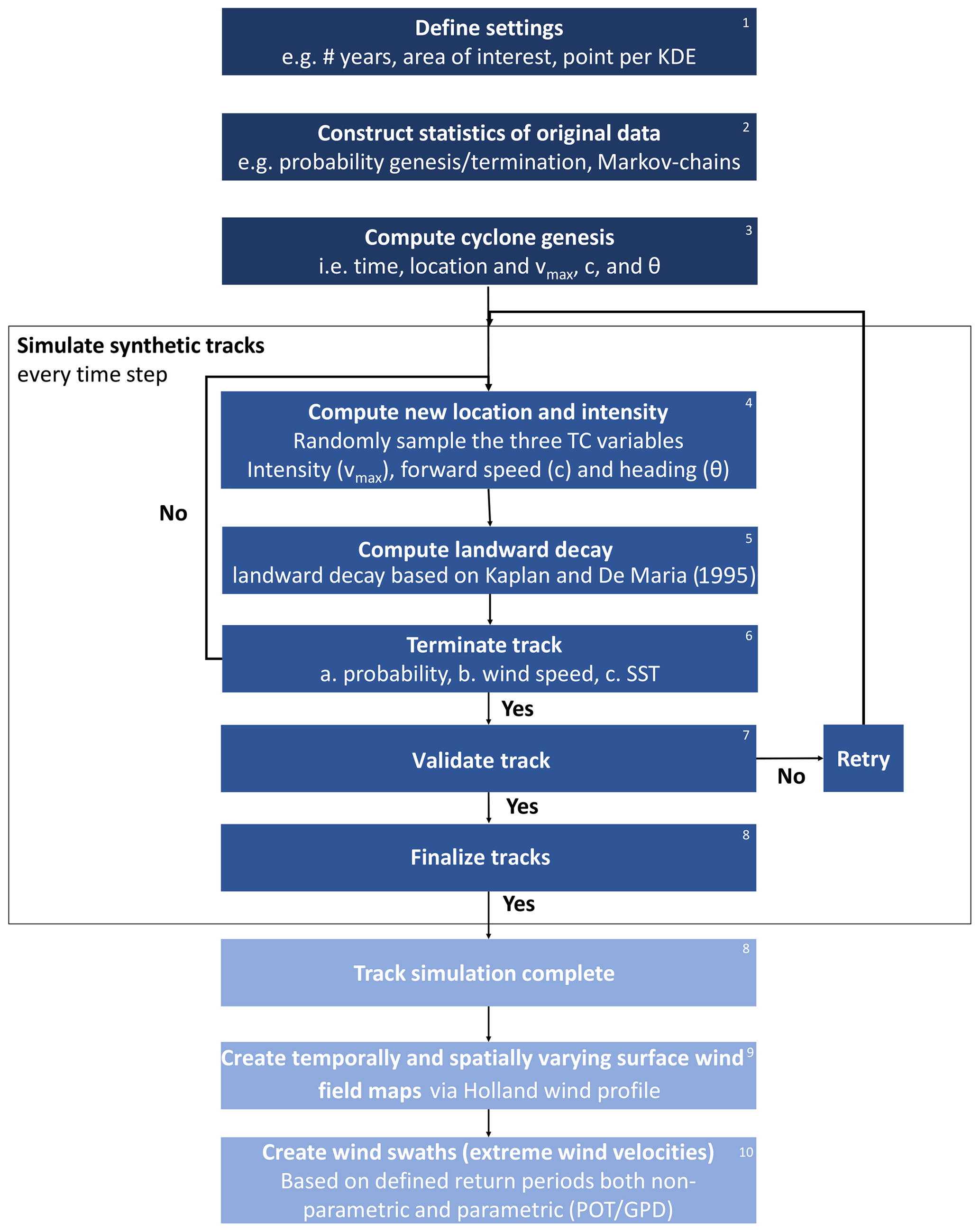
Figure 1Flowchart of the track modeling procedure. Dark blue colors are pre-processing steps, blue colors the computational core of TCWiSE and light blue post-processing steps. KDE stands for kernel density estimation, SST stands for sea surface temperature and POT/GPD is the acronym of peak over threshold and generalized Pareto distribution.
2.3 Track initialization
The track initialization is done through random sampling of the genesis locations for each track from a spatially varying probability constructed based on (historical) input data. Only the spatial occurrence of the genesis locations is sampled, as no temporal variability of genesis locations or other input parameters are included in genesis. The spatially varying probability used to sample the genesis locations is constructed by first drawing a rectangular grid of a user-definable size (default: ∘) around all historical events under consideration. For each grid point, all genesis locations within a certain distance (user-definable; default: 200 km) are counted and normalized with the total number of counted genesis points to obtain the genesis density at each grid point.
Genesis that occurred in ocean surface temperatures less than a user-definable value (default: 24 ∘C) are deleted since high SST is the driving force behind TC genesis, and without it TCs cannot occur (e.g., Gray, 1968). TCWiSE uses SST data from the International Research Institute of Columbia University (Reynolds et al., 2002), which provides a worldwide monthly average SST map at 1∘ resolution.
After generating the genesis locations, the matching timestamp, intensity and track propagation of genesis are determined. The timestamp is determined by applying a Poison distribution per year (i.e., the number of TCs per year varies from year to year), after which the within-the-year distribution is taken into account by giving each track a day number relative to 1 January of that year based on a KDE of historical data. The latter step allows taking into account average climatological patterns such as a higher number of TCs during the months of August and September. The intensity, heading and forward speed of the TC at the genesis location are determined by randomly sampling from all the historical occurrences at genesis within a certain (user-definable) distance. Hence, this sampling is using only the data points during TC genesis and results in initial values for intensity, heading and forward speed (and not changes to these variables as will be done for the track evolution).
2.4 Track evolution
After the generation of the genesis location and parameters, the evolution of the track and intensity is modeled during its lifetime in (by default) 3-hourly intervals. The propagation is modeled by sampling the change in the heading (Δθ), forward speed (Δc) and intensity (Δvmax) for each time step.
2.4.1 Search range
The KDE is constructed for each grid point based on input data within a specific search range. This search range is defined by a rectangular box of a user-definable size (default: ∘) around the point of interest. The minimum number of data points required within the search range is 250 (default, user-definable). If less than the specified amount of points is located within the search range, the search range is increased until the required number of data points is found or until the maximum is reached (user-definable; default: ).
The change in intensity evolution and track propagation, which includes the heading and forward speed, is all treated similarly. Changes are sampled from the pre-processed KDEs that are conditionally dependent on the previous time step. Historical occurrences are smoothed since a KDE from raw histograms is used (Wand and Jones, 1994). This smoothing overcomes possible discrete signals. By default, the heading is divided into 17 equally large bins and partly overlapping bins of 45∘, forward speed is divided into 17 overlapping bins of 2.5 kn and wind speed is divided into 37 overlapping bins of 5 kn. This ensures that the full parameter range for TCs is covered. For each variable, the search range (i.e., range for which values are included in the bin) is twice the window size (i.e., the difference per each subsequent bin) to ensure a smooth transition between different bins. All these settings are user-definable. Data points that are on land can be excluded in the computation of the intensity evolution.
No additional parameters are defined for the track evolution. Effects such as intensification, the Coriolis effect, wind shear and beta drift (Holland, 1983) are not explicitly defined nor controlled for. The conditionally dependent KDE of change per variable per location drives the complete track evolution.
2.4.2 Effect of land
When a TC makes landfall, TCs weaken due to, among other factors, a lack of heat sources (e.g., Tuleya, 1994). This effect should be part of the conditionally dependent KDE, but due to the possibly large search ranges per location (and thus blending of on-land and on-water conditions) the effect of land can be underestimated (and the intensity on water underestimated). Therefore, the user can exclude data points on land. When this is chosen, one should use additional formulations to reduce intensity when the synthetic TC is on land. Among other relationships available in the literature, Kaplan and DeMaria (1995) created a simple empirical model for computing cyclone wind decay after landfall. In TCWiSE, a similar method can be used to compute the decay of wind speed after landfall. Following the relationships of Kaplan and DeMaria, wind speed decreases exponentially based on how long a TC is on land. The specific amount of decay as a function of time is, again, user-definable.
2.4.3 Track termination
During each interval of 3 h, the tool checks if the tracks should be terminated. The termination criteria are defined in three different ways:
-
when the wind speed is lower than a user-definable low value (default 10 kn)
-
when the synthetic TC is over a user-definable low water temperature (default 10 ∘C)
-
the probability of termination based on (historical) input data.
When different methods of termination are used, the termination of a synthetic TC is thus not completely similar to the historical probability of termination. Hence, termination within TCWiSE can also be triggered by low wind speeds (due to the fact the TC is on land) and/or too-low SST.
2.4.4 Climate variability
Projected effects of climate change on frequency and intensity of TCs can also be taken into account via the heuristic implementation of a factor on both the frequency and intensity. These factors can be defined using expert assessment of TC climate predictions (e.g., Knutson et al., 2015), allowing, for instance, the assessment of changes in TC coastal hazards in the next century. The effect of climate variability on possible shifts of the TC tracks or regional changes of parameters are not included yet but could be included by modifying the (historical) KDEs or using global climate models as an input source for TCWiSE.
2.5 Temporally and spatially varying surface wind field
After the generation of the track (time, location and intensity), temporally and spatially varying wind fields are computed based on the parametric model of Holland et al. (2010) via the Wind Enhanced Scheme (WES; Deltares, 2018). The relationships of Nederhoff et al. (2019) are used either to compute the most probable TC geometry (RMW and radius of gale-force winds, also known as radius of 35 kn or R35) or to take geometry into account as a stochastic variable. The user has the choice between generic relationships and calibrations for different basins. This ensures reliable azimuthal wind speeds. TC asymmetry is considered based on Schwerdt et al. (1979) and assumes a constant inflow angle of 22∘ (Zhang and Uhlhorn, 2012). More details on the implementation of the Holland parametric wind model are provided in Deltares (2018).
2.6 Wind swaths
After the generation of the wind fields, wind swaths for different return periods are generated. Both non-parametric and parametric extremes based on a fitted POT/GPD for different return periods are computed. TCWiSE utilizes the POT method combined GPD (Caires, 2016) for extreme value analysis. In particular, the choice of the threshold for the POT and the fitting of the coefficients are automatically performed. Parametric estimates of extremes are preferred when statistical uncertainties need to be quantified or when fewer observations are available on which to base the non-parametric estimates.
3.1 Introduction
The United States (US) is one of the countries most affected by TCs over the years. In particular, the US Gulf Coast has suffered severely from hurricanes in the past, which have caused a significant number of casualties and a significant amount of damage. Among the most notorious, TCs Andrew in 1992, Katrina in 2005 and Harvey in 2012 devastated US territory. In the severe hurricane season of 2017 alone, Harvey, Irma and Maria resulted in more than USD 250 billion in damage in the US (NOAA, 2018).
In this section, a validation of generation, occurrence, propagation and termination of synthetic TC is carried out, by comparing with historical tracks for the entire NA basin. A more detailed comparison between historical BTD from the IBTrACS database and simulated synthetic tracks by TCWiSE is performed for nine control points in the GoM. Subsequently, extreme wind speed estimates from TCWiSE and from historical data are compared along the coastline and also validated against the literature. Figure 2 presents the area of interest for the validation case study, including relevant locations for this analysis.
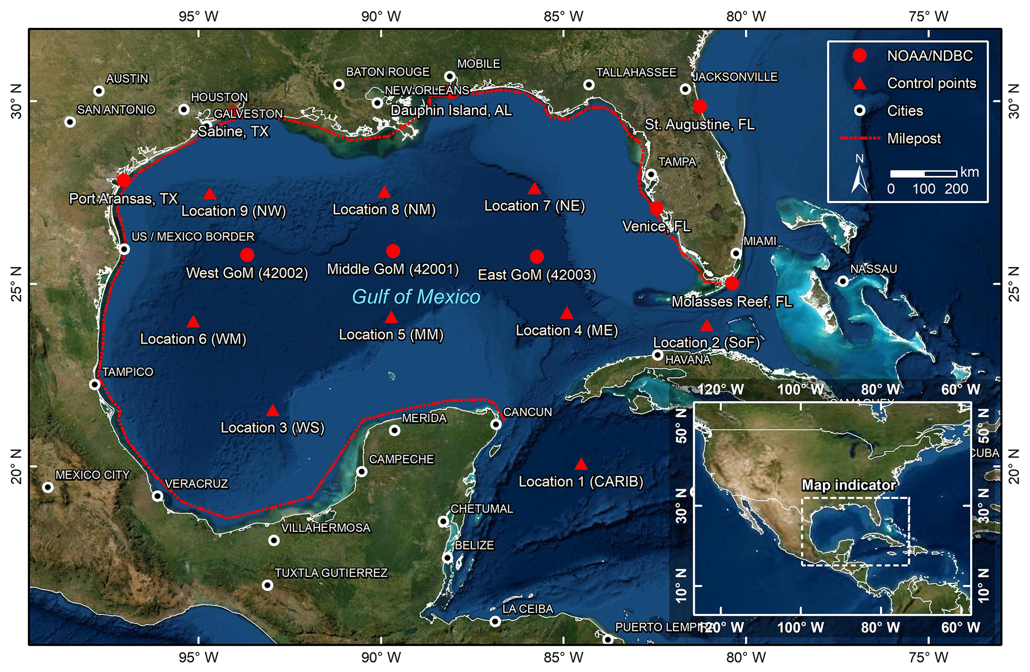
Figure 2Area of interest of the Gulf of Mexico, including the locations of the nine control points in the GoM (red triangles), NOAA/NDBC measurement location (red dots), cities (white circles) and milepost (red dashed line). © Esri, DigitalGlobe, GeoEye, Earthstar Geographics, CNES/Airbus DS, USDA, USGS, AeroGRID, IGN and the GIS User Community. Sect. 3.2.
3.2 Data
The NA basin data from the IBTrACS database are used within the TCWiSE algorithm to compute 10 000 years of synthetic TCs. Only historical data observed from 1886 up to 2019 are considered. The cutoff year of 1886 is chosen because of the increase in accuracy of the observation of the maximum wind speeds. This yields 955 historical TCs and 71 320 synthetic TCs for the entire NA basin.
Measured winds from a total of nine National Data Buoy Center (NDBC, https://www.ndbc.noaa.gov/, last access: 22 December 2019) buoys across the GoM have been used in this study to validate the TCWiSE-computed extreme wind speeds. Computed and observed wind speeds are all converted if needed to 10 m height and 10 min averaged (see, e.g., Harper et al., 2010). This is generally the height and the averaging period needed for hydrodynamic models (in wave modeling this is typically the 1 h average wind speed). Only observations from buoys with at least 20 years of data have been used to validate modeled wind speeds. Furthermore, only observations within a 200 km radius of an active TC (based on IBTrACS) are considered. This prevents the inclusion of peak wind speeds due to extra-tropical storms instead of TCs in the validation.
Moreover, TCWiSE-computed extreme values are compared to values found in the literature. For example, Vickery et al. (2009) present simulated TC-induced wind speeds across the US coastline for return periods of 50 up to 2000 years. Following the methodology of Neumann (1991), along the US coastline, NOAA (National Oceanic and Atmospheric Administration) presents hurricane return periods for both hurricanes (>64 kn) and major hurricanes (>96 kn) within 50 nautical miles (92.6 km) based on the track information. TCWiSE-computed return periods are compared to NOAA's reported values (https://www.nhc.noaa.gov/climo/, last access: 1 February 2019).
3.3 Validation computed vs. historic cyclone parameters
3.3.1 Statistical test for TC validation
A variety of tests are available for statistical comparison between computed and historical cyclone parameters. The tests are used to prove the hypothesis that the historical values come from the same statistical population as the simulated values. For each parameter, such as forward speed, a goodness of fit for the historical cumulative distribution function (CDF) can be performed and compared to the CDF from the synthetic tracks. Strictly, this would require that different datasets are employed for model fitting and for model testing so that distributional parameters of the model used to generate the large-sample CDF are not estimated from the historical sample. However, in this paper, we utilized all available observational data to include as much climate variability in the synthetic tracks as possible.
Several tests exist (e.g., Kolmogorov–Smirnov, Cramér–von Mises, Anderson–Darling, Kuiper, Watson) to test the null hypothesis that the samples' x and y come from the same (continuous) distribution (Stephens, 1974). In addition, a more pragmatic approach is available which consists of simply computing the mean absolute error (MAE) on the historical and computed CDFs. In this paper, we present a combination of different statistics to test if the synthetic tracks have similar statistical properties to the BTD. In particular, normalized mean absolute error (nMAE; MAE divided by variance of BTD), root-mean-square error (RMSE) and bias are presented. Additionally, the CDFs of several TCs physical properties are compared for the historical and synthetic tracks. Finally, the Kirchhofer (1974) method is used for quantifying similarities and differences in spatial patterns (e.g., TC genesis, evolution).
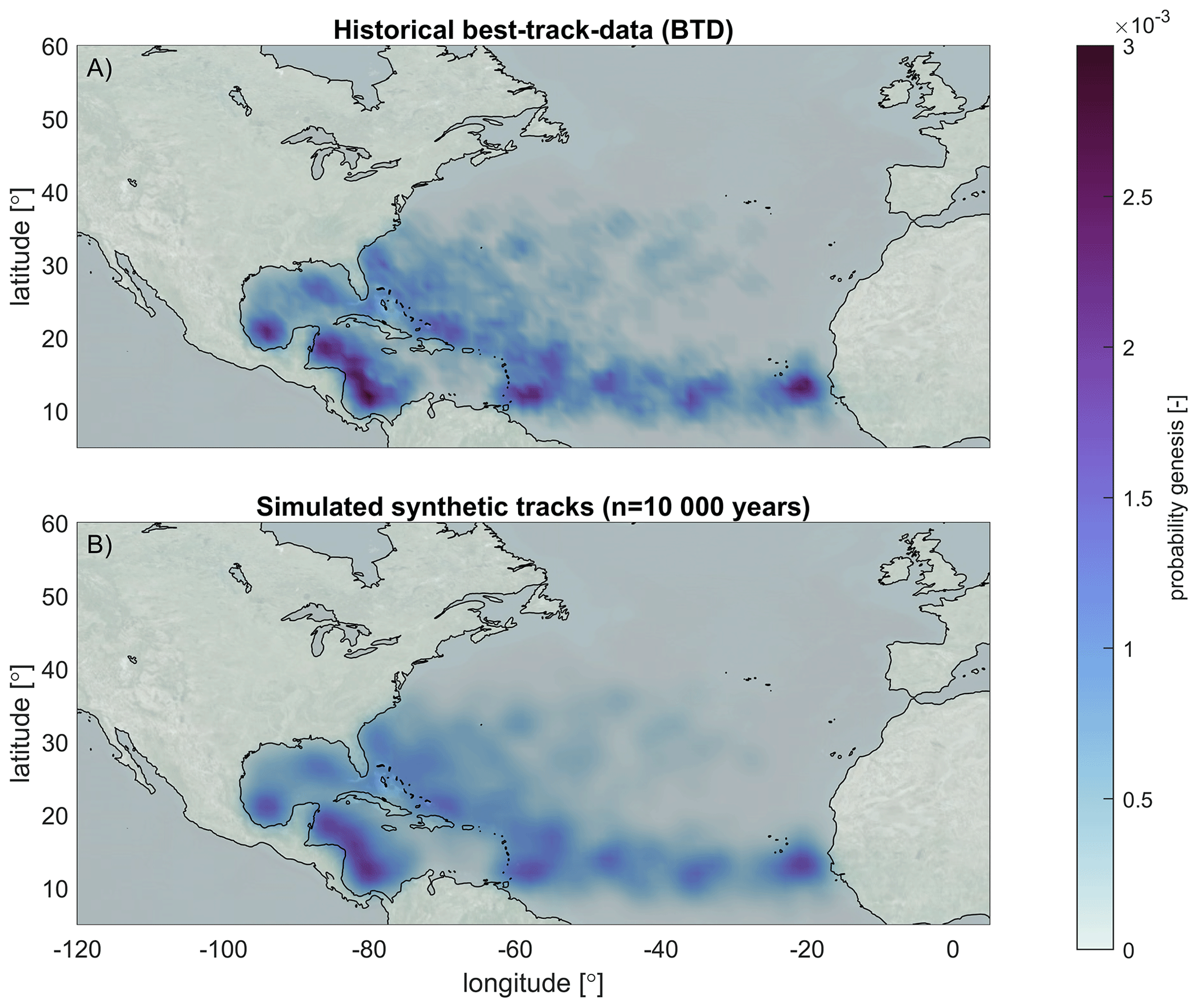
Figure 3Genesis probability of historical BTD (a) and simulated TCs with TCWiSE (b) for the NA basin. Occurrence is based on TCs within 200 km per grid cell for historical TCs from 1886–2019 and 10 000 years of simulated events. © Microsoft Bing Maps.
3.3.2 Computed and historic TC parameters
In the following section, the modeled results of TCWiSE are compared to historical BTD. Validation follows the life of a TC first with a visual and qualitative validation of the generation being presented. Subsequently, the track occurrence, evolution and CDFs of the three main parameters of TCWiSE are compared quantitatively to historical data. Lastly, a visual and qualitative validation of the termination is presented.
Generation
Historical and simulated genesis probability for the entire NA basin is shown in Fig. 3. Cyclone genesis is taken as the first point which the BTD identifies as such, which means it is the point from where meteorological institutes started tracking the storm. As shown in Fig. 3a, the simulated and the historical genesis match well visually. A hot spot of TC genesis is illustrated on the west coast of the African continent. Additionally, two hot spots are visible east of the Caribbean Sea and in the western part of the Caribbean. Within the GoM some areas also show cyclone genesis. The spatial patterns of genesis are almost identical, while being slightly smoothed out in the simulated synthetic tracks (Fig. 3b). This visual assessment was quantified and confirmed by using the Kirchhofer metric score, which provided a value equal to 0.967 (a value of 1.0 represents a perfect match). In particular, grid cells that are zero (either in the historical or synthetic dataset) are not taken into account in the analysis. This gives confidence that TCWiSE can reproduce the genesis patterns observed in the historical BTD.
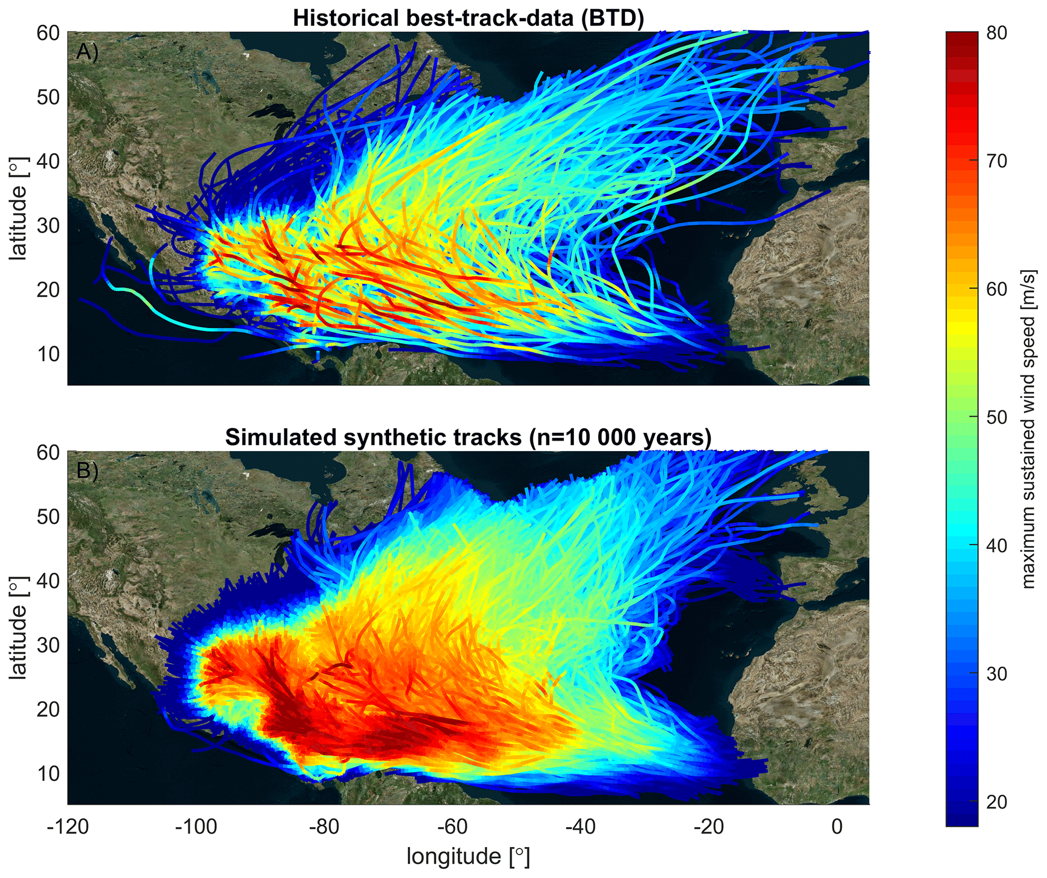
Figure 4(a) Overview of historical tropical cyclone tracks in the IBTrACS database for the period 1886–2019. (b) 10 000 years of simulated tracks with TCWiSE. Colors indicate the maximum intensity of the eye. Note that the maximum intensity is the maximum wind speed at the core of the TC, which is different from the temporally and spatially varying wind field and/or spatially varying wind swaths. In particular, further away from the TC eye, gale-force winds can still be present due to the TC. © Microsoft Bing Maps.
Track occurrence, evolution and CDFs
Historical and simulated TC intensity tracks are shown in Fig. 4. All individual tracks are plotted with a color code derived from the intensity of the eye of the storm (i.e., maximum sustained wind speed). Tracks with higher intensity are plotted on top of those with lower intensity. The figure shows that TCs are generated around latitudes of ±10–20∘ (see also Fig. 3). Some of the TCs increase in intensity while moving towards the northwest, making landfall in the US, in Central America, in the northern countries of South America and across the Caribbean. Others turn back in an eastward direction and propagate towards Europe. Intensities are generally larger in the Caribbean and GoM, while TCs that propagate northward decrease in intensity. Similar patterns can be observed in the simulated synthetic TCs (Fig. 4b). However, higher intensities can be observed for individual simulated synthetic tracks due to the larger number of years of data that are presented (10 000 years of simulated tracks vs. 134 years for the historical tracks) and thus a larger likelihood of having a more intense TC. Moreover, it does seem that synthetic TC tracks have a less clear southwest–northeast orientation in heading on the North Atlantic Ocean.
The average yearly occurrence of historical and synthetic TCs is presented in Fig. 5. A high occurrence of TCs in the GoM, in the Caribbean and along the east coast of the US is observed for both historical and simulated tracks. The simulated occurrence is quite similar but, as expected, more smoothened for the synthetic tracks. The Kirchhofer metric score for occurrence confirms the matching of the patterns with a high score of 0.926. This gives confidence that TCWiSE produces synthetic TCs with a similar occurrence rate to what has been historically observed.

Figure 5Average occurrence of historical BTD (a) and simulated TCs with TCWiSE (b) for the NA basin. Occurrence is based on TCs within 200 km per grid cell for historical TCs from 1886–2019 and 10 000 years of simulated events. © Microsoft Bing Maps.
The generation of synthetic TCs includes three distinct parameters that can be compared between the historical and synthetic tracks, namely forward speed (c), heading (θ) and maximum sustained wind speeds (vmax). The CDFs are presented for these parameters in Figs. 6 to 8 for the nine locations as shown on the map in Fig. 2. Visually the CDFs of the synthetic data appear to match those of the historical data rather well. nMAEs of the forward speed (Fig. 6) vary between 0.02–0.20 with an average RMSE of around 0.43 m s−1 and with a bias of +0.31 m s−1. Location 3 (WS) and location 9 (NW) have a larger error due to the positive bias. Statistical errors in the headings (Fig. 7) are generally small too. Locations 2 and 9 have larger nMAE than the other control locations (possibly due to the effect of land), while locations 7 and 8 have the lowest errors. The nMAE of maximum sustained wind speed (Fig. 8) varies between 0.00–0.04 with, on average, a RMSE of around 3.62 m s−1 and with a bias of −3.10 m s−1. These error statistics do reveal a general tendency for larger deviations closer to land but give confidence in the synthetic generation and propagation of the TC.
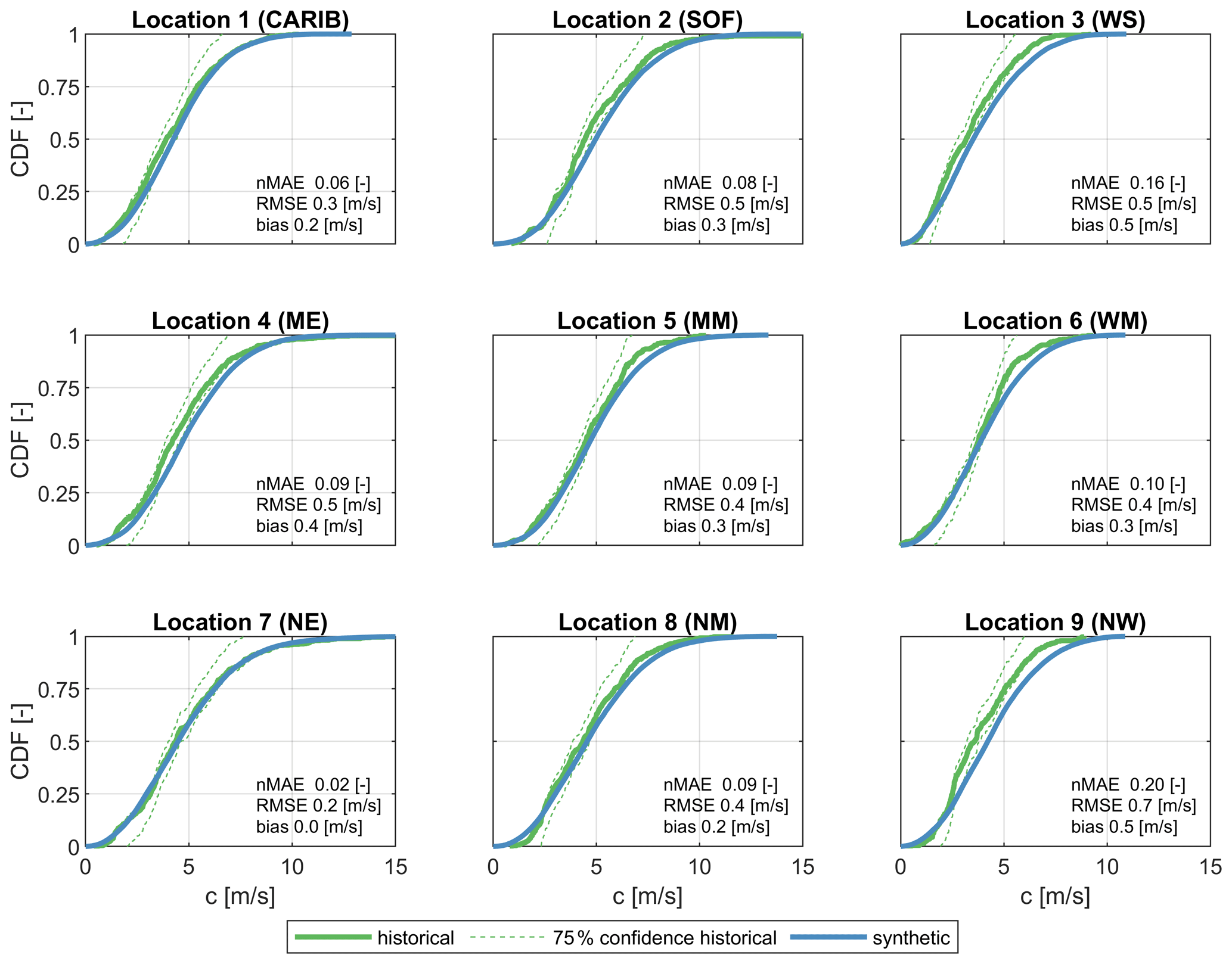
Figure 6CDFs of forward speed (c [m s−1]) of historical (green line) and synthetic (blue line) TCs at nine locations within the NA basin, as shown on the map in Fig. 2. The 75 % confidence interval (dashed green line) of historical data is also shown. Historic data are based on data available between 1886 and 2019, while synthetic data are derived from 10 000 years of simulated events with TCWiSE. Data points within 200 km from the control location are included in the analysis for both the historical and synthetic data.
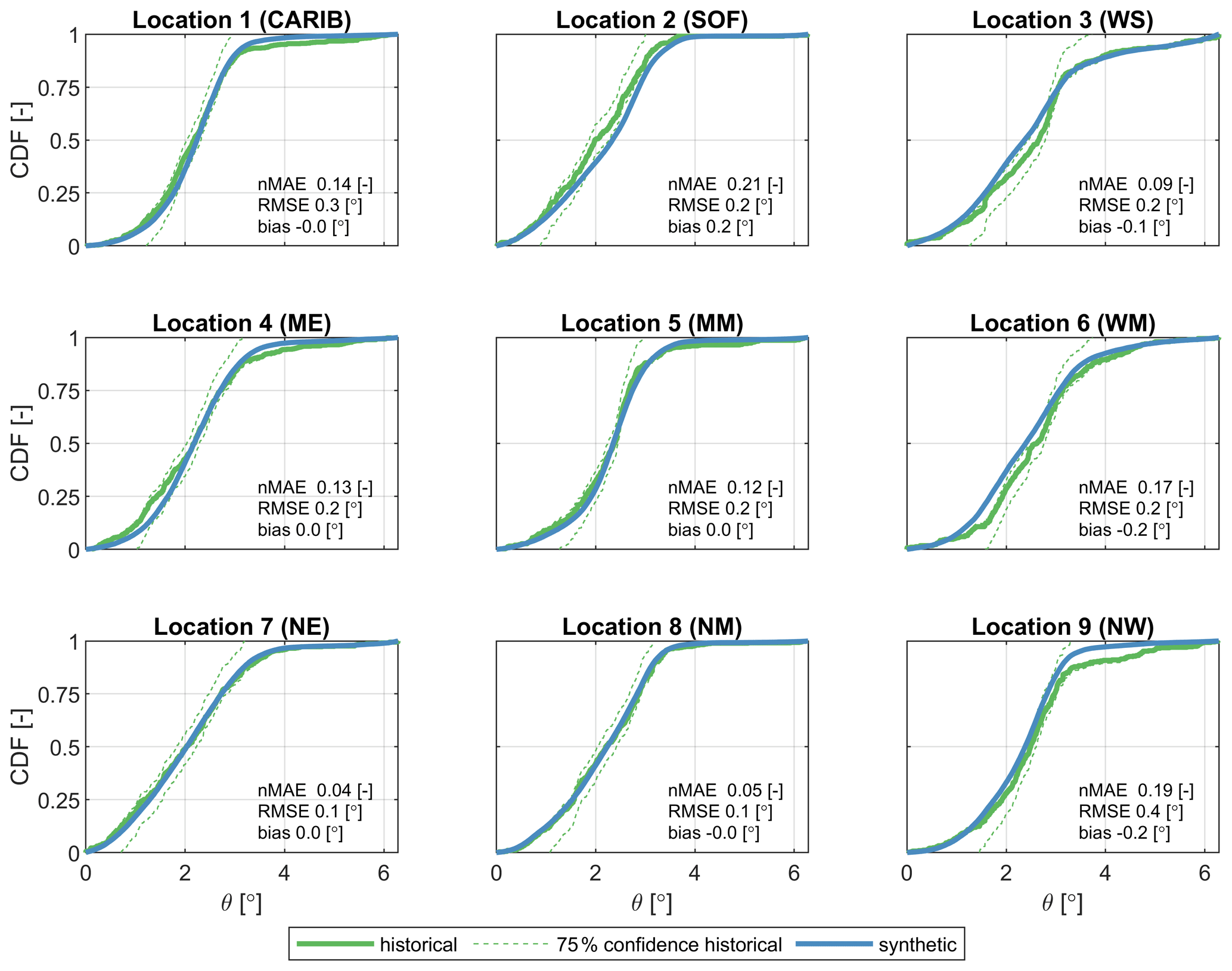
Figure 7CDFs of heading (θ [∘]) of historical (green line) and synthetic (blue line) TCs at 9 locations within the NA basin, as shown on the map in Fig. 2. The 75 % confidence interval (dashed green line) of historical data is also shown. Historic data are based on data available between 1886 and 2019, while synthetic data are derived from 10 000 years of simulated events with TCWiSE. Data points within 200 km from the control location are included in the analysis for both the historical and synthetic data.

Figure 8CDFs of maximum sustained wind speed (vmax [m s−1]) of historical (green line) and synthetic (blue line) TCs at nine locations within the NA basin, as shown on the map in Fig. 2. The 75 % confidence interval (dashed green line) of historical data is also shown. Historic data are based on data available between 1886 and 2019, while synthetic data are derived from 10 000 years of simulated events with TCWiSE. Data points within 200 km from the control location are included in the analysis for both the historical and synthetic data.
Track termination
Historical and simulated termination probability is shown in Fig. 9. In TCWiSE, cyclone termination is defined as the last point of TC that is obtained from the BTD. The figure shows that historically there is a large probability of termination at the east coast of Canada (i.e., Nova Scotia and the island of Newfoundland) (see, e.g., Elsner et al., 1999) and the east coast of Mexico. In some cases, TCs terminate after landfall in the US or while propagating on the Atlantic Ocean. Visually, the historical and simulated termination does not align as well. The reasons for deviations are that termination can be triggered by several different physical processes and is thus not so closely related to the input data. In particular, in TCWiSE, synthetic TCs can terminate due to a low ocean temperature or low wind speed on land. Hence, the differences in this comparison can be explained due to the schematization of the physical processes which lead to a different TC termination in TCWiSE than based on the historical probability alone. Also, errors from the previous steps in the TC life cycle (i.e., genesis location, propagation) will be compounded in the track termination. The comparison between historical and simulated termination probability was quantified by using the Kirchhofer metric score for termination, which provided a value of 0.622 (compared to 0.967 for genesis and 0.926 for occurrence).
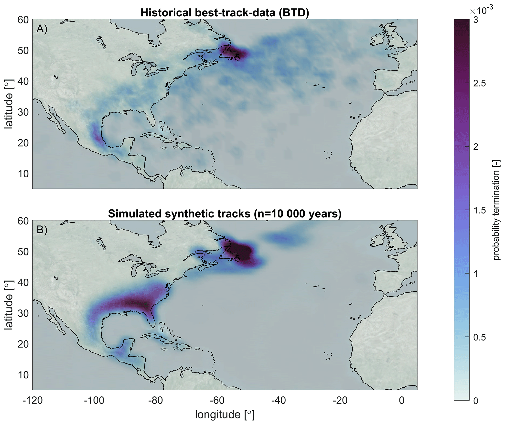
Figure 9Termination probability of historical BTD (a) and simulated TCs with TCWiSE (b) for the NA basin. Occurrence is based on TCs within 200 km per grid cell for historical TCs from 1886–2019 and 10 000 years of simulated events. © Microsoft Bing Maps.
3.4 Computed and historic TC maximum wind speeds
3.4.1 Observed extreme wind speeds
Figure 10 presents the non-parametric 10-year return value estimates of TC wind speed for the GoM based on synthetic TCs. Cooler colors depict lower TC wind speeds, and warmer colors higher wind speeds. The circles indicate the non-parametric estimates based on buoy observations for the same return period; given that the observations cover about 40 years, they are the fourth-highest ever recorded value. The figure shows how the general patterns of higher wind speeds in the central GoM and lower values near land, as shown by the data, are reproduced correctly by TCWiSE. The model-computed values are biased high (i.e., overestimation) for stations near land. This is most likely due to land-related processes not being fully accounted for in TCWiSE. Also, the data scarcity (sub-sampling) affects the estimates from the observations.
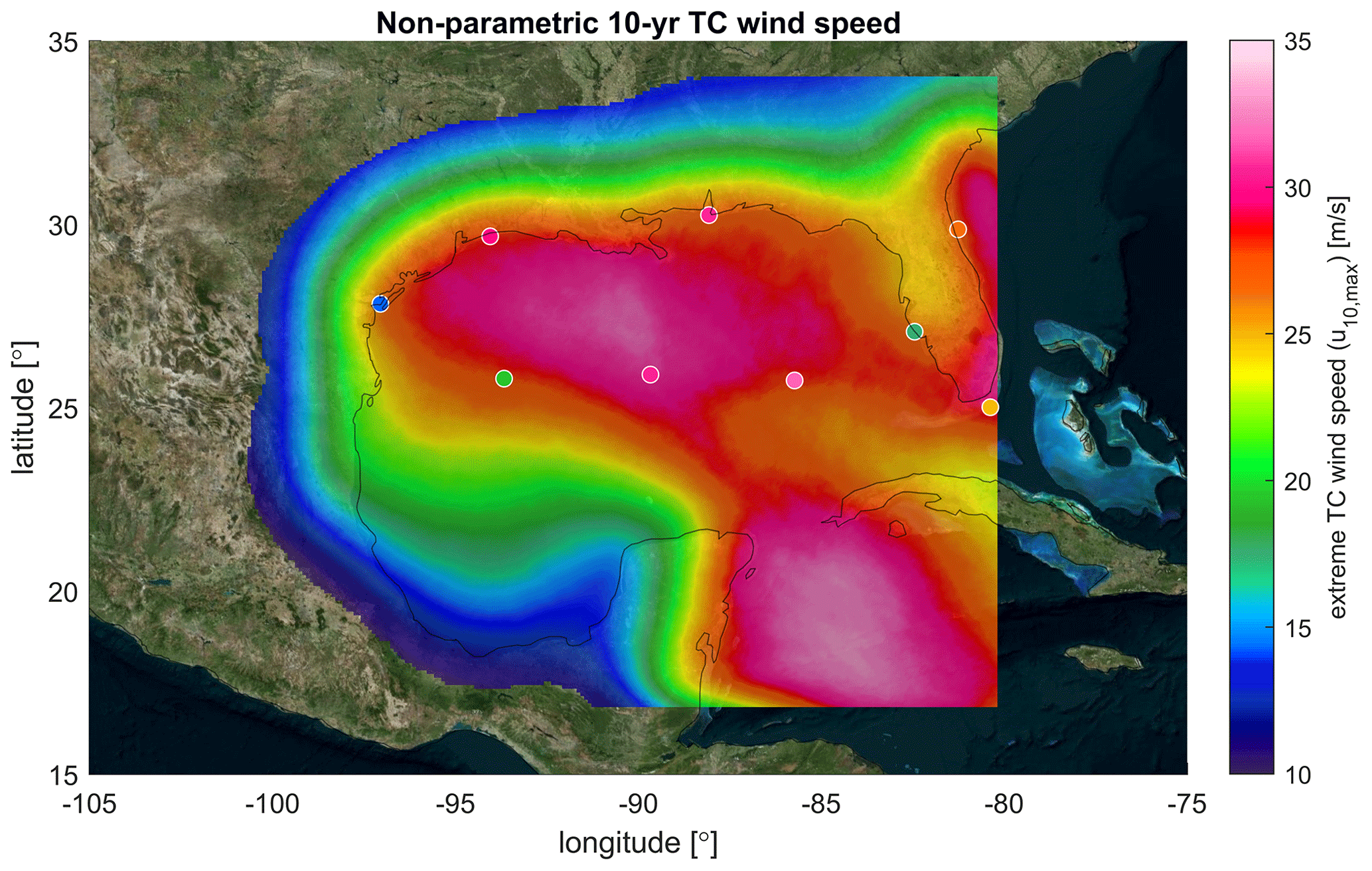
Figure 10Model estimates for non-parametric empirical estimate of 10-year TC wind speed return values based on extreme wind speeds based on 10 000 years of TCWiSE computations. The white circles indicate observed TC wind speed extremes based on NDBC wave buoys and NOAA data. All wind speeds are in meters per second, 10 min averaged and determined at a 10 m height. © Microsoft Bing Maps.
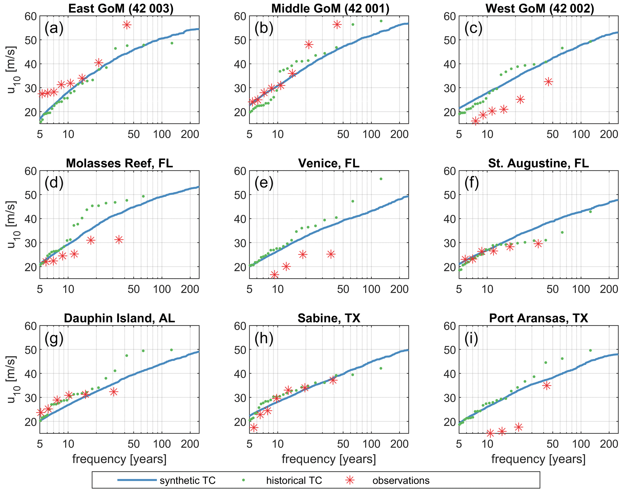
Figure 11Observed and TCWiSE-computed TC extreme wind speeds for different return periods. Red stars are observed events from NDBC and NOAA wave buoys. Green dots are historical TCs based on BTD and the Holland wind profile, and blue line are synthetic modeled events based on synthetic tracks and the Holland wind profile. All wind speeds are in meters per second, 10 min averaged and determined at a 10 m height).
Figure 11 presents a comparison between observed and TCWiSE-computed TC extreme wind speeds, for different return periods, at nine locations throughout the GoM, both based on 134 years of historical and 10 000 years of synthetic tracks. As could already be seen in Fig. 10, there is some scatter between observed, historical and synthetic TC wind speeds. For example, the peak in the observed wind speed, in particular that of larger return periods, in the east GoM (Fig. 11a) and middle GoM (Fig. 11b) are underestimated by both the historical and synthetic TCs. These are respectively peaks corresponding to Hurricane Rita (2005) and Hurricane Kate (1985). Based on the observation record of 40 years, the non-parametric return period estimate is 40 years, whereas TCWiSE indicates that the return period associated with those events is higher. The cause of the large difference between observed wind speeds and values derived from historical and synthetic TCs wind speed for the west GoM (Fig. 11c) is unclear. On the other hand, wind speed extremes at Venice, FL (Fig. 11e), and Port Aransas, TX (Fig. 11i), seem to be overestimated by the historical and synthetic TCs, which could be related to unresolved land-related processes.
3.4.2 Modeled extreme wind speeds
Figure 12 presents the 1000-year parametric TC wind speed for the GoM, estimated by fitting a GPD to the POT of the generated data. The figure shows a spatial pattern similar to that of the 10-year non-parametric TC wind speeds (Fig. 10). The highest values are found in the Caribbean Sea and central GoM. Lower values can be found in northwest Florida and in the southwest of the GoM. This is in line with the literature (e.g., Neumann, 1991). Computed occurrence rates are also in line with NOAA values for both hurricanes (>64 kn) and major hurricane (>96 kn) within 50 nautical miles (92.6 km). Occurrence rates for major hurricanes (>96 kn) are the highest for south Florida and Louisiana, with a respective return period of 17–20 years. TCWiSE estimates are 19–22 years.
Figure 13 presents the estimated TC wind speed return value swaths versus coastal milepost which starts at Cancún, Mexico and goes across the GoM in a clockwise orientation. Several return periods are depicted in different colors. Moreover, TC wind speed is presented both averaged over 10 min in units of meters per second and averaged over 1 min in units of knots. The SSHWS is included as well. TCWiSE simulation indicates for a return period of 10 years TC wind speed of around 30 m s−1 (close to SSHWS-1) near Cancún and large stretches of the US coastline. For a return period of 1000 years, this increases to values around 60 m s−1 (around SSHSS-4). Generally, values near Villahermosa are the lowest for all of the GoM. Vickery et al. (2009) reported maximum gust TC wind speeds with a return period of 100 years that vary between 33–57 m s−1 (using a conversion factor of 1.23 based on Harper et al., 2010). TCWiSE indicates values on the same order of magnitude but with less spatial variability.
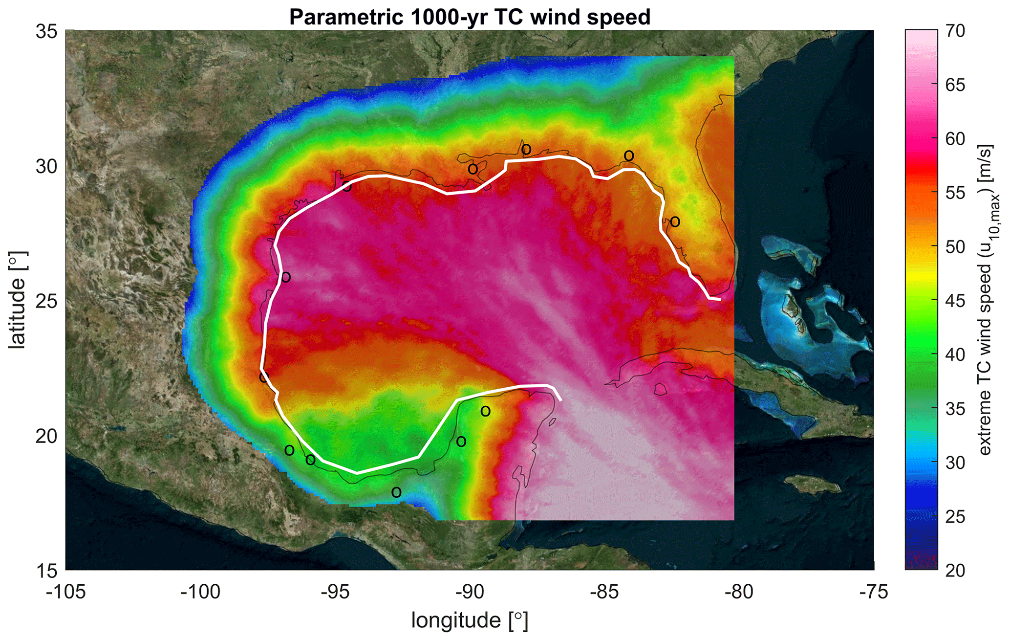
Figure 12Model estimates for the parametric empirical estimate of 1000-year TC wind speed return values based on extreme wind speeds based on 10 000 years of TCWiSE computations. All wind speeds are in meters per second, 10 min averaged and determined at a 10 m height. Black dots are the location of cities as plotted in Figs. 10 and 13. © Microsoft Bing Maps.
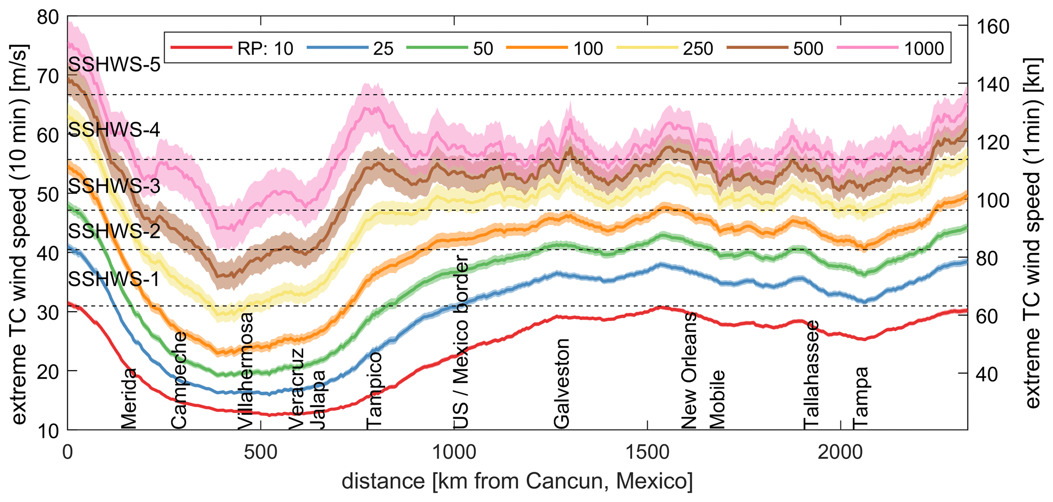
Figure 13TCWiSE 10-, 25-, 50-, 100-, 250-, 500- and 1000-year return value estimates of wind speed. All wind speeds are in meters per second, 10 min averaged and determined at a 10 m height (left axis) or 1 min averaged in knots (right axis). Cities on the x axis are also depicted in Fig. 12 as black circles. Milepost is presented in the same figure as a white line. Shading shows the 5–95 % confidence interval. SSHWS value indicates the corresponding Saffir–Simpson hurricane wind scale.
For clarity, discussion points have been grouped under three main topics: the TCWiSE tool, validation study and computational performance.
4.1 The TCWiSE tool
The philosophy which guided the development of TCWiSE is to release an open-source tool, giving modelers full control over the track generation, propagation and termination. However, this makes TCWiSE also more sensitive to input errors compared to pre-generated global synthetic TC data products (e.g., Bloemendaal et al., 2020). However, the strength of this approach is 2-fold. First of all, this allows the user of TCWiSE to rigorously calibrate and validate assumptions within the code for the user's own case study site. Secondly, due to the flexible MATLAB coding language, it allows easy adjustments of the tool and implementation of additional processes. For example, stochastic rainfall was recently added to the original code by Bader (2019).
TCWiSE is an almost completely data-driven tool to simulate synthetic TCs. As such, output values are highly dependent on the (historical) input data and not the physical processes describing the genesis, propagation and termination of these TCs. This limits the possibility of synthetic TCs computed by TCWiSE that are physically credible but statistically unlikely. Moreover, this assumes stationarity of the historical record. If cyclone characteristics are expected to behave identically to the last decades, this method has been proven accurate for the determination of extremes. However, climate change is expected to influence the frequency and intensity of future TCs (e.g., Knutson et al., 2010). This can already be accounted for by a heuristic factor to adjust both the frequency and intensity of the TC (or other variations implemented by the user) to reflect changes due to climate change. Other ways to account for this – such as by adjusting the KDE, applying data-driven probabilities of TC genesis as a function of SST and/or further use of datasets derived by global climate models – are currently being investigated.
The effect of land on intensity can be taken into account either directly via the conditionally dependent KDE or landward decay based on De Maria and Kaplan (1995). The latter is beneficial since TC information on land contaminates the KDE of intensity. In particular, due to the applied search range methodology, information from decreasing winds on land start to affect winds on the water. The downside of this method is that this does introduce an additional calibration coefficient for the user and larger deviations in the termination. Moreover, TCWiSE does not include a boundary layer model, which means that the physical wind response to variable surface drag and terrain height is not included. In particular, the at-sea TC wind will extend inland before the TC center crosses the coast and the decay turns on. Done et al. (2020) have shown, however, that the output of parametric wind models can be used to simulate the near-surface wind swaths of landfalling TCs, accounting for terrain effects such as coastal hills and abrupt changes in surface roughness due to coastlines and forested or urban areas.
In TCWiSE, track termination can be either be purely based on historical track termination or via additional formulations based on user-definable cut-off wind speed and/or SST. While these additional formulations were of importance to get the track evolution (and thus associated coastal hazards) simulated correctly, they do result in deviations of simulated track termination compared to historical data. However, arguably, track termination is not of importance for the simulation of coastal hazards, and therefore this is deemed an acceptable trade-off for the more reproductive skill in the track evolution.
TCWiSE does not take into account errors in the wind fields or the associated impact on the confidence interval for the computed return periods for wind speeds. Nederhoff et al. (2019) demonstrated that the Holland wind profile in combination with reliable estimates of the TC geometry (i.e., the radius of maximum wind and gale-force winds) to calibrate the wind profile wind has a median root-mean-square difference of 2.9 m s−1. Other approaches (e.g., Vickery et al., 2009) do include error estimates in their estimates of the extreme winds. Vickery et al. (2009) conclude that uncertainty in the estimated 100-year return period wind speed varies by around 6 %, which corresponds to about ±3–5 m s−1.
4.2 Validation study
Validation results across the NA basin and in particular the GoM have shown that TCWiSE can reproduce the main patterns seen in the BTD, wind observations and literature. This can be done despite the lack of physical description of the climate dynamics given that TCWiSE is a purely data-driven tool and does not include specific processes to steer TC propagation.
A comparison of similarities in spatial patterns between synthetic tracks and historic tracks, evaluated by means of the Kirchhofer metric score, shows that TCWiSE is able to correctly reproduce genesis and TC occurrence, while differences were found for the TC termination. These differences can be attributed to TC termination, which can get triggered by several criteria in TCWiSE. Hence, it is not just related to the historical probability of termination. At the same time, this has a relatively minor effect on the track evolution and consequently coastal hazards.
The comparison of CDFs of forward speed, heading and maximum sustained wind speed of historical and synthetic tracks shows a good agreement for the different stations in general. While differences between observed and modeled CDFs are apparent, results of the goodness-of-fit tests are generally acceptable (Figs. 6–8), with a mean nMAE of 0.08. More classical statistical tests such as Kolmogorov–Smirnov were not presented here and often reject the null hypothesis that the observed and modeled data are from the same distribution. This is related to the methodology of providing inputs to the Markov chains. While this method resulted in reliable probability distributions, it also smoothed out some local spatial patterns and therefore resulted in differences at the nine control locations. Arguably, locally patterns in the BTD (features <500 km) could well be subject to a sampling error and not necessarily a feature of the TC climate we aim to reproduce.
All BTD, since 1866, have been included as a basis for the generation of synthetic tracks. Especially for pre-satellite records, errors in the BTD can be quite significant, so previous studies (e.g., Holland, 2008) selected a specific subset of the BTD to ensure the quality of the data and remove potential inconsistencies. However, the advantage of including all data entries is that the derived TC climate is more widely defined (i.e., larger parameter space). But it is easily possible in TCWiSE to only include tracks from more recent years.
4.3 Computational performances
To provide the reader with a rough estimate of the computation performance of the tool, TCWiSE simulations for the NA and in particular GoM were performed on a 16-core Windows machine. The simulation of 10 000 years of synthetic tracks took several hours. The generation of temporally and spatially varying wind fields, wind swaths and matching extreme value analysis took another ±15 d.
A new methodology and highly flexible open-source tool have been developed with which synthetic TCs can be generated and used for subsequent analysis of (coastal) hazards. In particular, TCWiSE handles track initialization, evolution and termination based on historical TC information. Subsequently, the tool creates a temporally and spatially varying wind field based on the Holland wind profile calibrated for TC geometry. Lastly, TCWiSE computes non-parametric and parametric wind swaths for user-definable return periods.
The validation study for the NA and in particular the GoM showed reliable skill in terms of track initialization and evolution compared to the historical BTD. A more detailed assessment of the goodness of fit at nine control locations showed that normalized errors are generally smaller than 10 %. Extreme wind speeds show agreement for more frequent return periods, with possible deviation for the most extreme cases. This is the result of biases associated with the scarcity of observed data.
TCWiSE can be useful in a variety of applications. Improved estimates of extreme TC conditions can lead to a better quantification of coastal hazards (e.g., extreme storm surge levels and waves) and consequent risks and damages resulting from these hazards. Similarly, an improved assessment of those hazards can help guide the design of appropriate adaptation measures. Other fields of application may vary from improved design parameters for offshore structures to navigation. In all these types of applications, the flexibility of TCWiSE to tailor the synthetic TC generation to user-specific needs and questions makes the tool very well suited for coastal engineers. The application of the tool for determining coastal hazards will be presented as part of a separate paper currently under preparation.
TCWiSE is freely available for other researchers and consultants. The repository consists of the MATLAB code and required input data (such as BTD and SST) map. Registration is required before getting access to the subversion. Please go to https://www.deltares.nl/en/software/tcwise/ (Deltares, 2021) for more information and registration.
KN, TL, JH and MvO developed the MATLAB code for computing synthetic tropical cyclone tracks. SC and AG supported the development of the idea and the writing of the paper.
The authors declare that they have no conflict of interest.
The authors thank Deepak Vatvani for all his inspiring cyclone work over last decades at Deltares and Bjorn Robke for Fig. 2. The authors also would like to thank reviewers James Done and Lorenzo Mentaschi for their comments and help on improving this paper. Final thanks are due to Patrice Lucas for proofreading the article and providing valuable comments, which have led to an improved paper.
This research has been supported by Deltares internal research programs “Flood Risk Strategies”, “Planning for disaster risk reduction and resilience”, “Offshore Engineering” and “Extreme Weather Events”.
This paper was edited by Gregor C. Leckebusch and reviewed by James Done and one anonymous referee.
Arthur, W. C.: A statistical-parametric model of tropical cyclones for hazard assessment, Nat. Hazards Earth Syst. Sci. Discuss. [preprint], https://doi.org/10.5194/nhess-2019-192, in review, 2019.
Bader, D. J.: Including stochastic rainfall distributions in a probabilistic modelling approach for compound flooding due to tropical cyclones, Delft University of Technology, available at: http://resolver.tudelft.nl/uuid:57b9e495-0c90-4cf5-ab22-e169fb908ac1 (last access: 1 March 2018), 2019.
Bloemendaal, N., Haigh, I. D., de Moel, H., Muis, S., Haarsma, R. J., and Aerts, J. C. J. H.: Generation of a global synthetic tropical cyclone hazard dataset using STORM, Sci. Data, 7, 1–19, https://doi.org/10.1038/s41597-020-0381-2, 2020.
Brzeźniak, Z. and Zastawniak, T.: Basic Stochastic Processes, Springer, London., 2000.
Caires, S.: A Comparative Simulation Study of the Annual Maxima and the Peaks-Over-Threshold Methods, J. Offshore Mech. Arct., 138, 051601, https://doi.org/10.1115/1.4033563, 2016.
Coles, S.: An introduction to statistical modeling of extreme values, Springer-Verlag, London, 2001.
de Lima Rego, J., Winsemius, H., and Minns, T.: Mozambique, 2017 – Coastal Flooding Hazard Assessment, Deltares Report 1230818-000-ZKS-007 (for World Bank's Global Facility for Disaster Reduction and Recovery; GFDRR), Deltares, the Netherland, 2017.
Deltares: Wind Enhancement Scheme for cyclone modelling – User Manual, Version 3.01, Deltares, the Netherlands, 2019, 214, 2018.
Deltares: TCWiSE, available at: https://www.deltares.nl/en/software/tcwise/, 26 February 2021.
Done, J. M., Ge, M., Holland, G. J., Dima-West, I., Phibbs, S., Saville, G. R., and Wang, Y.: Modelling global tropical cyclone wind footprints, Nat. Hazards Earth Syst. Sci., 20, 567–580, https://doi.org/10.5194/nhess-20-567-2020, 2020.
Elsner, J. B., Elsner, T. M. G. J. B., and Kara, A. B.: Hurricanes of the North Atlantic: Climate and Society, Oxford University Press, available at: https://books.google.com/books?id=Pa-I-7UFMHAC (last access: 1 February 2020), 1999.
Emanuel, K., Ravela, S., Vivant, E., and Risi, C.: Supplement to A Statistical Deterministic Approach to Hurricane Risk Assessment, B. Am. Meteorol. Soc., 87, S1–S5, https://doi.org/10.1175/bams-87-3-emanuel, 2006.
Giardino, A., Nederhoff, K., and Vousdoukas, M.: Coastal hazard risk assessment for small islands: assessing the impact of climate change and disaster reduction measures on Ebeye (Marshall Islands), Reg. Environ. Change, 18, 2237–2248, https://doi.org/10.1007/s10113-018-1353-3, 2018.
Gray, W. M.: A global view of the origin of tropical disturbances and storms, Mon. Weather Rev., 96, 669–700, 1968.
Harper, B. A., Kepert, J. D., and Ginger, J. D.: Guidelines for converting between various wind averaging periods in tropical cyclone conditions, World Meteorol. Organ, October, available at: https://library.wmo.int/doc_num.php?explnum_id=290 (last access: 1 February 2020), 2010.
Hoek, J.: Tropical Cyclone Wind Statistical Estimation In Regions with Rare Tropical Cyclone Occurrence, Delft University of Technology, available at: https://repository.tudelft.nl/islandora/object/uuid%3A2986959f-53ce-42a6-9299-c24833353616 (last access: 1 February 2020), 2017.
Holland, G. J.: Tropical cyclone motion: environmental interaction plus a beta effect., J. Atmos. Sci., 40, 328–342, https://doi.org/10.1175/1520-0469(1983)040<0328:TCMEIP>2.0.CO;2, 1983.
Holland, G.: A Revised Hurricane Pressure–Wind Model, Mon. Weather Rev., 136, 3432–3445, 2008.
Holland, G. J., Belanger, J., and Fritz, A.: A Revised Model for Radial Profiles of Hurricane Winds, Mon. Weather Rev., 138, 4393–4401, https://doi.org/10.1175/2010MWR3317.1, 2010.
James, M. K. and Mason, L. B.: Synthetic tropical cyclone database, J. Waterw. Port, Coast., 131, 181–192, https://doi.org/10.1061/(ASCE)0733-950X(2005)131:4(181), 2005.
Kaplan, J. and DeMaria, M.: A Simple Empirical Model for Predicting the Decay of Tropical Cyclone Winds after Landfall, J. Appl. Meteorol, 34, 2499–2512, https://doi.org/10.1175/1520-0450(1995)034<2499:ASEMFP>2.0.CO;2, 1995.
Kernkamp, H. W. J., Van Dam, A., Stelling, G. S., and De Goede, E. D.: Efficient scheme for the shallow water equations on unstructured grids with application to the Continental Shelf, Ocean Dynam., 61, 1175–1188, https://doi.org/10.1007/s10236-011-0423-6, 2011.
Kirchhofer, W.: Classification of European 500 mb Patterns, Arbeitsbericht der Schweiz. Meteorol. Zurich Zent., 1974.
Knapp, K. R., Kruk, M. C., Levinson, D. H., Diamond, H. J., and Neumann, C. J.: The international best track archive for climate stewardship (IBTrACS), B. Am. Meteorol. Soc., 91, 363–376, https://doi.org/10.1175/2009BAMS2755.1, 2010.
Knutson, T. R., Tuleya, R. E., Garner, S. T., Bender, M. A., Vecchi, G. A., Held, I. M., and Sirutis, J. J.: Modeled Impact of Anthropogenic Warming on the Frequency of Intense Atlantic Hurricanes, Science, 327, 454–458, https://doi.org/10.1126/science.1180568, 2010.
Knutson, T. R., Sirutis, J. J., Zhao, M., Tuleya, R. E., Bender, M., Vecchi, G. A., Villarini, G., and Chavas, D.: Global projections of intense tropical cyclone activity for the late twenty-first century from dynamical downscaling of CMIP5/RCP4.5 scenarios, J. Climate, 28, 7203–7224, https://doi.org/10.1175/JCLI-D-15-0129.1, 2015.
Lee, C. Y., Tippett, M. K., Sobel, A. H., and Camargo, S. J.: An environmentally forced tropical cyclone hazard model, J. Adv. Model. Earth Sy., 10, 223–241, https://doi.org/10.1002/2017MS001186, 2018.
Lesser, G. R., Roelvink, J. A., van Kester, J. A. T. M., and Stelling, G. S.: Development and validation of a three-dimensional morphological model, Coast. Eng., 51, 883–915, https://doi.org/10.1016/j.coastaleng.2004.07.014, 2004.
Nederhoff, K., Giardino, A., van Ormondt, M., and Vatvani, D.: Estimates of tropical cyclone geometry parameters based on best-track data, Nat. Hazards Earth Syst. Sci., 19, 2359–2370, https://doi.org/10.5194/nhess-19-2359-2019, 2019.
Neumann, C. J.: NOAA Technical Memorandum NWS NHC 38: The National Hurricane Center Risk Analysis Program (HURISK), NHC: Costliest U.S. tropical cyclones tables updated, NOAA Tech. Memo. NWS NHC-6, 3, available at: https://www.nhc.noaa.gov (last access: 1 February 2020), 1991.
NOAA: Costliest U.S. tropical cyclones tables updated, NOAA Tech. Memo. NWS NHC-6, 3, available at: https://www.nhc.noaa.gov/pdf (last access: 1 February 2020), 2018.
Reynolds, R. W., Rayner, N. A., Smith, T. M., Stokes, D. C., and Wang, W.: An Improved In Situ and Satellite SST Analysis for Climate, J. Climate, 15, 1609–1625, https://doi.org/10.1175/1520-0442(2002)015<1609:AIISAS>2.0.CO;2, 2002.
Schwerdt, R. W., Ho, F., and Watkins, R. R.: Meteorological criteria for standard project hurricane and probable maximum hurricane windfields, gulf and east coasts of the United States, NOAA Technical Report NWS 23, September, 1979.
Stephens, M. A.: Stephens_EDF Statistics and some comparisons, J. Am. Stat. Assoc., 69, 730–737, 1974.
Tuleya, R. E.: Tropical storm development and decay: sensitivity to surface boundary conditions, Mon. Weather Rev., 122, 291–304, https://doi.org/10.1175/1520-0493(1994)122<0291:TSDADS>2.0.CO;2, 1994.
Vickery, P. J. and Twisdale, L. A.: Prediction of hurricane wind speeds in the united states, J. Struct. Eng., 121, 1691–1699, https://doi.org/10.1061/(ASCE)0733-9445(1995)121:11(1691), 1995.
Vickery, P. J., Skerlj, P. F., Steckley, C., and Twisdale, L. A.: Hurricane wind field model for use in hurricane simulations, J. Struct. Eng., 126, 1203–1221, 2000.
Vickery, P. J., Wadhera, D., Twisdale, L. A., and Lavelle, F. M.: U.S. Hurricane Wind Speed Risk and Uncertainty, J. Struct. Eng., 135, 301–320, https://doi.org/10.1061/(ASCE)0733-9445(2009)135:3(301), 2009.
Wand, M. P. and Jones, M. C.: Kernel Smoothing, Chapman and Hall, Boca Raton, FL, U.S., available at: http://oro.open.ac.uk/28198/ (last access: 1 February 2020), 1994.
Zhang, J. A. and Uhlhorn, E. W.: Hurricane Sea Surface Inflow Angle and an Observation-Based Parametric Model, Mon. Weather Rev., 140, 3587–3605, https://doi.org/10.1175/mwr-d-11-00339.1, 2012.