the Creative Commons Attribution 4.0 License.
the Creative Commons Attribution 4.0 License.
 | 23 Feb 2021
Typhoon rainstorm simulations with radar data assimilation on the southeast coast of China
Jiyang Tian
Ronghua Liu
Liuqian Ding
Liang Guo
Bingyu Zhang
As an effective technique to improve the rainfall forecast, data assimilation plays an important role in meteorology and hydrology. The aim of this study is to explore the reasonable use of Doppler radar data assimilation to correct the initial and lateral boundary conditions of the numerical weather prediction (NWP) systems. The Weather Research and Forecasting (WRF) model is applied to simulate three typhoon storm events on the southeast coast of China. Radar data from a Doppler radar station in Changle, China, are assimilated with three-dimensional variational data assimilation (3-DVar) model. Nine assimilation modes are designed by three kinds of radar data and at three assimilation time intervals. The rainfall simulations in a medium-scale catchment, Meixi, are evaluated by three indices, including relative error (RE), critical success index (CSI), and root mean square error (RMSE). Assimilating radial velocity at a time interval of 1 h can significantly improve the rainfall simulations, and it outperforms the other modes for all the three storm events. Shortening the assimilation time interval can improve the rainfall simulations in most cases, while assimilating radar reflectivity always leads to worse simulations as the time interval shortens. The rainfall simulations can be improved by data assimilation as a whole, especially for the heavy rainfall with strong convection. The findings provide references for improving the typhoon rainfall forecasts at catchment scale and have great significance on typhoon rainstorm warning.
- Article
(13283 KB) - Full-text XML
- BibTeX
- EndNote


Although the resolution of numerical weather prediction (NWP) systems is increasing with the improvement of computational efficiency and abundance of observation data, rainfall is still one of the most difficult meteorological factors to forecast (Lu et al., 2017; Avolio and Federico, 2018). A typhoon always comes with heavy rainfall which leads to great loss. However, due to the uncertainty of the rainfall and the imperfect generation of NWP systems, rainfall forecast with severe convection is unsatisfactory in medium and small catchment scales (Tian et al., 2017a). Data assimilation plays an important role in NWP and is always applied to correct the initial and lateral boundary condition of NWP systems, which can effectively improve the rainfall forecast (Mohan et al., 2015; Liu et al., 2018).
Various kinds of observation data have been tested and assimilated by different assimilation methods. Wan and Xu (2011) simulated a heavy rainstorm using the Weather Research and Forecasting (WRF) model with the Gridpoint Statistical Interpolation (GSI) data assimilation (DA) system in the central Guangdong Province of southeast China. The rainfall simulation error was reduced at 4 km grid scale by assimilating satellite radiance data, which helped to analyze rainfall causes accurately. Giannaros et al. (2016) evaluated a lightning data assimilation (LTNGDA) technique over eight rainfall events occurring in Greece. The verification scores of the rainfall simulations were significantly improved by the employment of the WRF-LTNGDA scheme, especially for heavy rainfall. Zhang et al. (2013) presented a regional ensemble data assimilation system that assimilated microwave radiances into the WRF model for hydrological applications. The rainfall simulations were improved in terms of the accumulated rainfall and spatial rainfall distribution in the southeastern United States. Yucel et al. (2015) assimilated conventional meteorological data by a three-dimensional variational data assimilation (3-DVar) model into the coupled atmospheric–hydrological system. The rainfall simulations, as well as the runoff simulations, improve significantly in large basins in the western Black Sea region of Turkey.
Due to their high spatiotemporal resolution, radar data are assimilated to correct the NWP system for mesoscale and microscale weather prediction (Milan et al., 2008; Zhao and Jin, 2008). Wang et al. (2013) tested the four-dimensional variational data assimilation (4-DVar) system by simulating a midlatitude squall-line case in the US Great Plains, and the results indicated that radar data assimilation was able to improve rainfall forecasts from the WRF model at the convective scale. Liu et al. (2013) selected four storm events in a small catchment (135.2 km2) located in southwest England to explore the effect of data assimilation for rainfall forecasts based on the WRF model, and assimilating radar reflectivity by the 3-DVar model can significantly improve the forecasting accuracy for the events with one-dimensional evenness in either space or time. By using the WRF model and Advanced Regional Prediction System (ARPS) 3-Dvar, Hou et al. (2015) improved the short-term forecast skill by up to 9 h by assimilating radar data in southern China.
Most studies focus on the assimilation algorithm and data selection. However, consistent conclusions have not been obtained for the option of radar reflectivity and radial velocity, and few studies pay attention to the time interval setting of data assimilation. Based on the WRF and 3-DVar models, Tian et al. (2017b) found that radar reflectivity assimilation led to better rainfall simulations than radial velocity assimilation at the time interval of 6 h. Maiello et al. (2014) assimilated both radar reflectivity and radial velocity by the 3-DVar model with a 3 h assimilation cycle to improve the WRF high-resolution initial conditions, and the rainfall forecast became more accurate for several experiments in the urban area of Rome. Bauer et al. (2015) used the WRF model in combination with the 3-DVar scheme to estimate the rainfall simulations, and the results showed that radar data assimilation significantly improved the rainfall simulations by a 1 h Rapid Update Cycle at the high resolution of 3 km in Germany.
In reality, the operational forecasts from meteorological departments are guidance forecasts with a large forecasting area. It is impossible to focus on the accuracy of the rainfall in small and medium catchment scales. Limited computing power means that the number of restarting times for the forecasting system is only 2–4 times per day (Xie et al., 2016). The forecasting accuracy descends gradually as the run time goes on because the data assimilation is not in real time. Due to the poor accuracy at small scales and low resolutions, the rainfall forecasting from the meteorological department cannot be used directly as the input for hydrological forecasting in small and medium catchments (Tian et al., 2019). The local meteorological observations are necessary to be assimilated to improve the high-resolution rainfall forecast. The NWP model may not be corrected in a timely manner at a long time interval of data assimilation, while shortening the time interval needs a lot of computational resources, and the observation errors in local meteorological observations may also be amplified with high assimilation frequency in the NWP model.
China suffers approximately nine tropical cyclones (TCs) each year on average (Shen et al., 2017). Most TCs develop into typhoons which always bring huge economic losses and a great number of casualties. Fujian is one of the most regularly affected provinces on the coastline of southeast China, and heavy rainfall caused by the interaction of typhoons and complex terrain leads to severe flood disasters. Accurate rainfall forecasting is of great significance to flood control and disaster mitigation. However, typhoon rainstorms are still difficult to predict (Li et al., 2019). There are eight Doppler radar stations to obtain full coverage for meteorological monitoring in Fujian Province. The plentiful radar data provide convenience and a basis for the exploration of radar data assimilation at catchment scale.
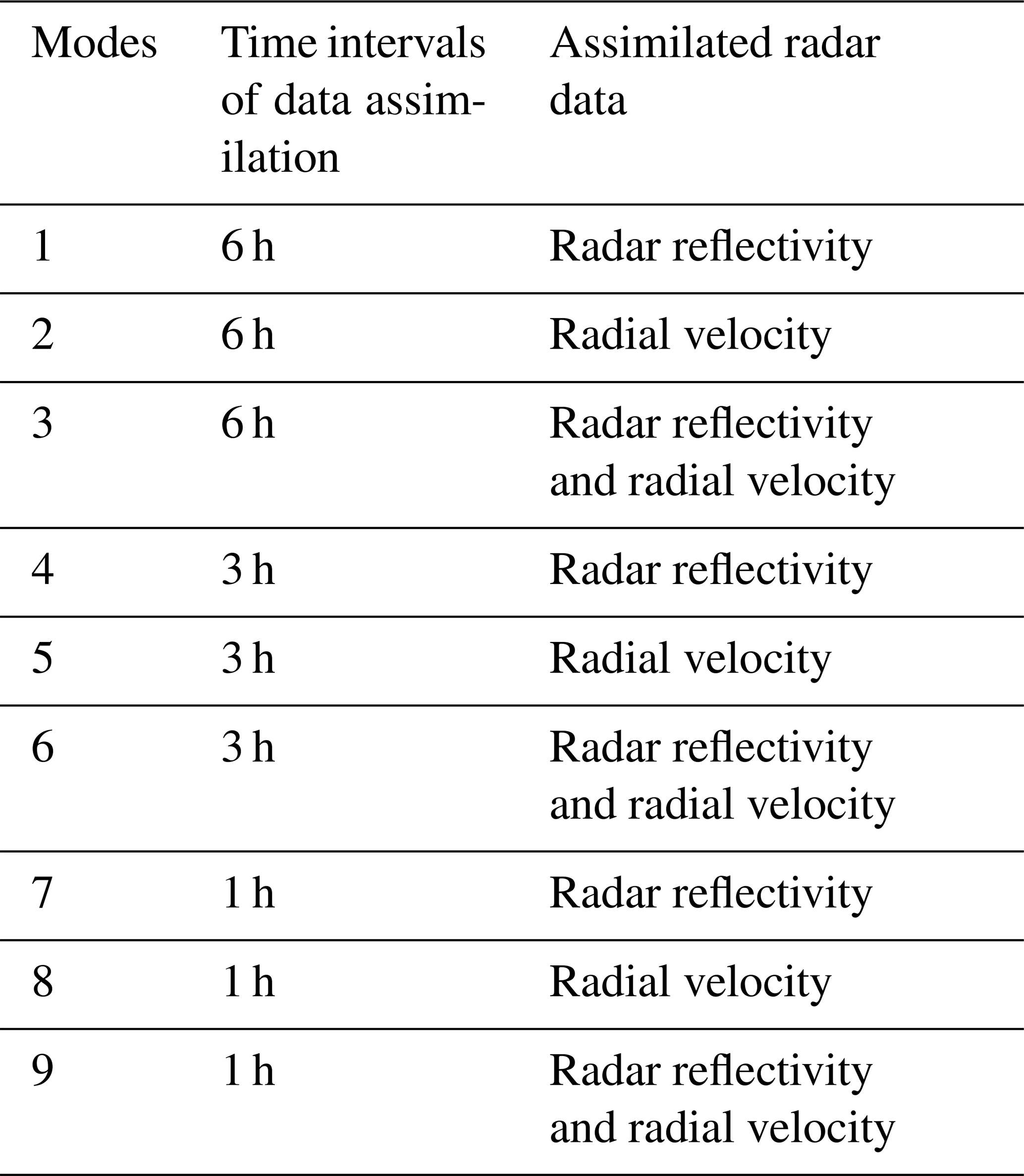
In this study, Meixi catchment located in Fujian Province is chosen as the study area. Due to the frequent heavy rainfall, flood disasters are up more than 20 times since 1949. On 9 July 2016, heavy rainfall caused by typhoon Nepartak led to severe flooding and attracted strong interest from the public, academics, and government. Accurate rainfall simulations have a great practical significance in the study area. In order to explore the reasonable use of Doppler radar data assimilation to correct the initial and lateral boundary conditions of the NWP systems, the WRF model is applied to simulate three typhoon storm events affecting the Meixi catchment, and the 3-DVar model is used to assimilate the radar data to improve the typhoon rainstorm simulations. Nine assimilation modes are designed by three kinds of radar data (radar reflectivity, radial velocity, and radar reflectivity and radial velocity) and at three assimilation time intervals (1, 3, and 6 h). The rainfall simulations are evaluated by three indices, including relative error (RE), critical success index (CSI), and root mean square error (RMSE).
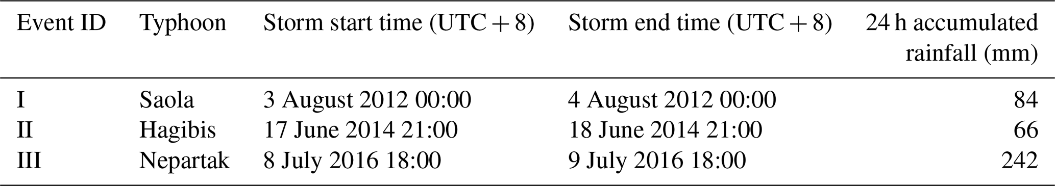
The Meixi catchment lies in central-eastern Fujian Province with a subtropical monsoon climate (Fig. 1). The drainage area is 956 km2, and the average annual rainfall is approximately 1560 mm. There are eight rain gauges and one hydrologic station (Fig. 2). In order to investigate the radar data assimilation effects on rainfall simulations, different kinds of rainfall processes caused by different stages of the typhoons are chosen in Meixi catchment. Three rainfall storms are shown in Table 1. Saola formed on 28 July 2012 and landed at Fuding, Fujian, by 3 August. Then Saola weakened into a tropical storm at Jiangxi. With the movement of Saola, Meixi catchment was not directly affected, and the accumulated 24 h rainfall was only 84 mm. Hagibis landed at Shantou, Guangdong, on 15 June 2014 and then moved toward the north at a fast-moving speed. Fortunately, Hagibis weakened into a tropical depression quickly while moving to northeastern Fujian on 17 June. Event II occurred after the typhoon passed Meixi catchment, and the accumulated 24 h rainfall was only 66 mm. Nepartak reached Fujian on 9 July 2016 and strengthened at Putian. Then Nepartak moved towards the northwest at a fast-moving speed, and event III occurred when Nepartak was close to Meixi catchment. During the period, Nepartak reached its peak intensity. The 24 h accumulated rainfall was 242 mm, which led to a high peak flow of 4710 m3 s−1 in Meixi catchment. The most destructive flood caused water and power outages in 11 villages and towns. Official figures stand at 74 dead and 15 missing from the flood, which also caused a direct economic loss of CNY 5.234 billion. Accurate rainfall forecasts appeared to be particularly important for Meixi catchment.

Figure 1The location of the Meixi catchment and three nested domains.
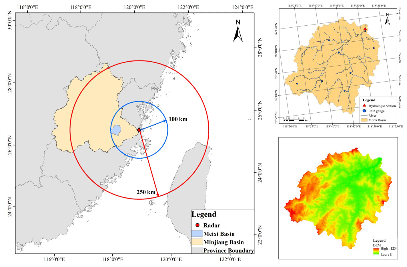
Figure 2Radar scan area and Meixi basin.
3.1 Model description
3.1.1 WRF model and configurations
As the latest-generation mesoscale NWP system, the WRF model in version 4.0 is used to simulate the three typhoon storm events. Three nested domains (Dom 1, Dom 2, and Dom 3) with two-way nesting are designed and centered over Meixi catchment. The grid spacings are set at 4, 12, and 36 km for the three nested domains from inside to outside (Chen et al., 2017). The grid numbers for the nested domain sizes are 100×100 for Dom 1, 210×210 for Dom 2, and 300×300 for Dom 3 (Fig. 1). Meixi catchment is completely covered by the innermost domain. All domains are comprised of 40 vertical pressure levels with the top level set at 50 hPa (Maiello et al., 2014). The NCEP Final (FNL) Operational Global Analysis data with grids are used to drive the WRF model and provide the initial and lateral boundary conditions. The time step is set to be 1 h for the WRF model output. The spin-up period of 12 h is applied to obtain a more accurate rainfall simulation. The option of physical parameterizations has a significant effect on the rainfall simulations, especially for microphysics, planetary boundary layer (PBL), radiation, land surface model (LSM), and cumulus physics (Otieno et al., 2019). According to the previous studies on physics options selection, WRF Single-Moment 6 (WSM 6) for microphysics, Yonsei University (YSU) for PBL, the Rapid Radiative Transfer Model for application to GCMs (RRTMG) for longwave and shortwave radiation, Noah for LSM, and Kain–Fritsch (KF) for cumulus physics are adopted in this study (Srivastava et al., 2015; Hazra et al., 2017; Cai et al., 2018; Tian et al., 2021).

3.1.2 The 3-DVar data assimilation and observation operator
The fundamental aim of the 3-DVar data assimilation is to produce an optimal estimate of the true atmospheric state by the iterative solution of a prescribed cost function (Ide et al., 1997):
where x is the vector of the analysis, xb is the vector of first guess or background, y is the vector of the model-derived observation that is transformed from x by the observation operator H, i.e., y=H(x), and y0 is the vector of the observation. B is the background error covariance matrix, and R is the observational and representative error covariance matrix. Equation (1) shows that the 3-DVar is based on a multivariate incremental formulation. Velocity potential, total water mixing ratio, unbalanced pressure, and stream function are all preconditioned control variables. Radial velocity has already been derived into component winds that are the same as the analysis variables; hence, radial velocity can be assimilated directly by Eq. (1). However, radar reflectivity assimilation needs an additional forward operator that associates the model hydrometeors with the radar reflectivity. Due to the wide applicability, the matrix of CV3 is adopted in this study to simplify the data assimilation procedure (Meng and Zhang, 2008).
The observation operator H in Eq. (1) links the model variables to the observation variables. For radar reflectivity, the observation operator is shown as follows (Sun and Crook, 1997):
where Z is the radar reflectivity (in dBZ), ρ is the density of air (in kg m−3), and qr is rainwater mixing ratio (in g kg−1). Equation (2) is derived by assuming a Marshall–Palmer raindrop size distribution and that the ice phases have no effect on reflectivity.
For radial velocity, the model-derived radial velocity Vr can be calculated as follows (Tian et al., 2017b):
where u, v, and w are the three-dimensional wind field, x, y, and z represent the location of the observation point, and xi, yi, and zi represent the location of the radar station; ri is the distance between the location of a data point and the radar station, and vt is the hydrometeor fall speed or terminal velocity. According to Sun and Crook (1998), vt can be given by
where a is the correction factor, is the base-state pressure, and p0 is the pressure at the ground.
3.2 Numerical experiments
3.2.1 Assimilation modes
An S-band Doppler weather radar located at Changle can completely cover Meixi catchment. The observation radius of Changle radar reaches 250 km, and the distance between Meixi catchment and the radar station is less than 100 km (Fig. 2), which makes the quality of radar data credible. The assimilated data – radar reflectivity and radial velocity – can be obtained once every 6 min continuously. All the radar data with quality control are provided by the newest generation weather radar network of China (CINRAD/SC). The observation error standard deviations of radar reflectivity and radial velocity are set 2 dBZ and 1 m s−1 in the 3-DVar model, respectively (Caya et al., 2005). The radar data assimilation modes are designed by three kinds of radar data (radar reflectivity, radial velocity, and radar reflectivity and radial velocity) and at three assimilation time intervals (1, 3, and 6 h). The rainfall simulation without data assimilation is used as the control mode. Nine modes are shown in Table 3.
Table 3Radar data assimilation modes designed with data types and time intervals.
3.2.2 WRF cycling runs for data assimilation
In order to obtain the whole process of the rainfall simulations, the running time is set at 3, 42, and 36 h for storm events I, II, and III, respectively. As shown in Fig 3, the cycling runs are set according to the time interval of data assimilation, and run 1 can be regarded as the WRF run without data assimilation. The dashed line segment represents the model spin-up. The first guess generated by run 1 is applied to drive run 2. As time progresses, the first guess file generated in the previous run is used to provide the initial conditions for the following run. For storm event I, data assimilation starts on 3 August 2012 at 00:00 (all times are UTC+8) and occurs at intervals of 6, 3, and 1 h. The start time of data assimilation is 18:00 on 17 June 2014, and the end time is 00:00 on 18 June 2014 for storm event II. Data assimilation takes place on 8 July at 18:00 and ends on 9 July at 18:00 at intervals of 6, 3, and 1 h for storm event III.
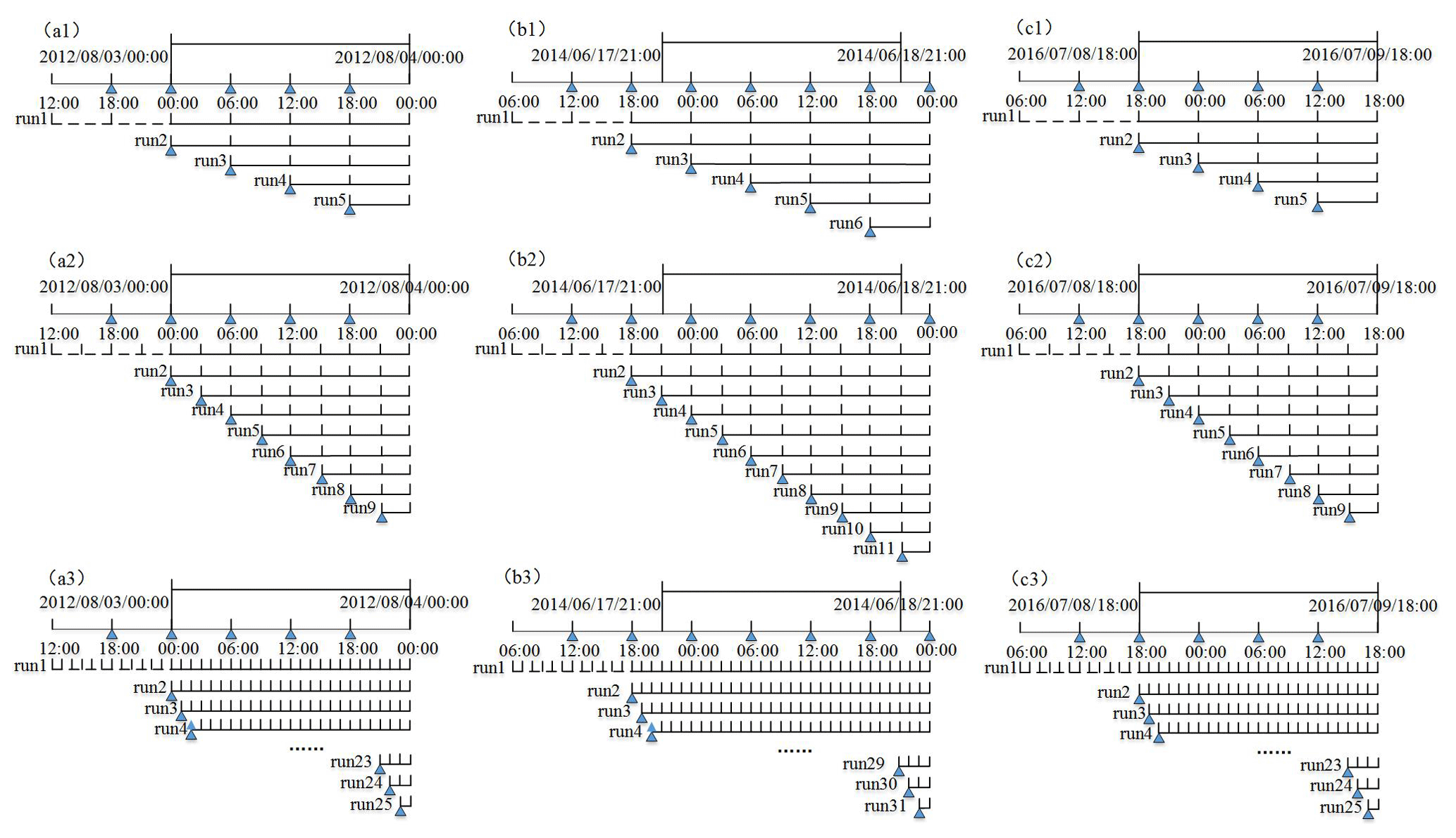
Figure 3The time bars of the assimilation cycling runs for (a) storm event I, (b) storm event II, and (c) storm event III.
In this study, the observation of areal rainfall in Meixi catchment is averaged by the eight stations with the Thiessen polygon method (Sivapalan and Blöschl, 1998), while the simulation of areal rainfall is averaged from all grids of the WRF model inside the Meixi catchment. The relative error (RE) is used to evaluate the total rainfall amount simulation:
where P′ is the simulation of 24 h accumulated areal rainfall, and P is the observation of 24 h accumulated areal rainfall.
The spatiotemporal patterns of the rainfall simulations are evaluated by the critical success index (CSI) and modified root mean square error (m-RMSE), which is defined as the ratio of root mean square error (RMSE) to the mean values of the corresponding observations (Liu et al., 2012; Prakash et al., 2014; Agnihotri and Dimri, 2015):
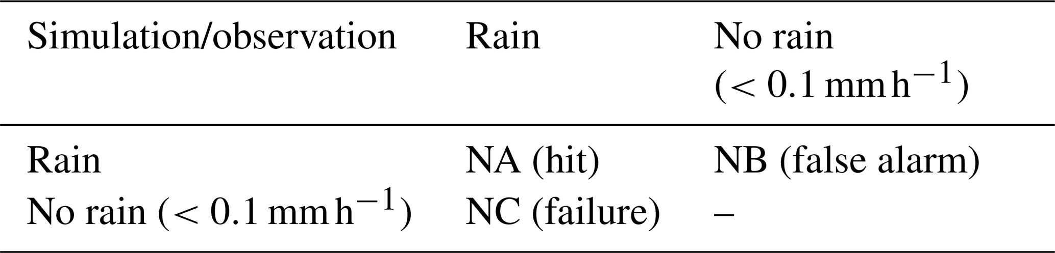
The CSI is calculated based on the rain or no rain contingency table (Dai et al., 2019). Table 4 shows that rainfall<0.1 mm h−1 as the threshold is regarded as no rain. In order to evaluate the simulation of spatial rainfall distribution by CSI, NAi, NBi, and NCi at each time step i (i=1 h) are calculated by comparing the rainfall observation with the simulation extracted at eight rain gauge locations, and then the values of NAi, NBi, and NCi at all time steps are averaged to produce the final verification results. Therefore, N refers to the total time steps (N=24). For temporal dimension evaluation, NAi, NBi, and NCi are first calculated using the time series data of simulations and observations at each rain gauge i (i=1), then the averaged index values of all rain gauges are regarded as the final verification results. Thus instead of the simulation time steps, N represents the total number of the rainfall gauges (N=8) for temporal dimension evaluation. The perfect score of CSI is 1.
Table 4Rain/no rain contingency table for the WRF simulation against observation.
The m-RMSE is calculated using Eq. (8). For spatial dimension evaluation, and Pj refer to the simulation and observation of 24 h accumulated rainfall at rain gauge j, respectively. M is the total number of rain gauges (M=8). For temporal dimension evaluation, and Pj are the simulation and observation of areal rainfall at each time j, respectively. M represents the total amount of time (M=24). The perfect score of RMSE is 0.
5.1 Accumulated rainfall simulations of the nine data assimilation modes
Nine data assimilation modes for three storm events are evaluated by RE for 24 h accumulated areal rainfall. The average values of the RE (ARE) of the three storm events for each mode are also calculated. As shown in Table 5, data assimilation modes make the rainfall simulations worse according to the REs of event I. Only mode 8 has the closest rainfall simulation to the observation in the nine data assimilation modes, and the RE is below 1 %. For event II, all data assimilation modes can improve the accumulated rainfall simulations, while for event III, most modes make the accumulated rainfall simulations better except for modes 2 and 3. Mode 8, i.e., assimilating radial velocity at a time interval of 1 h, always has the lowest RE and performs the best. The improvement of the rainfall simulations is the most obvious for event III, and the rainfall magnitude is quite close to the observation, which has important significance in torrential rainfall forecasts and catastrophic flood forecasts in medium and small basins.
Table 5Accumulated rainfall simulation values (mm) and RE values (%) of the nine data assimilation modes for three storm events.
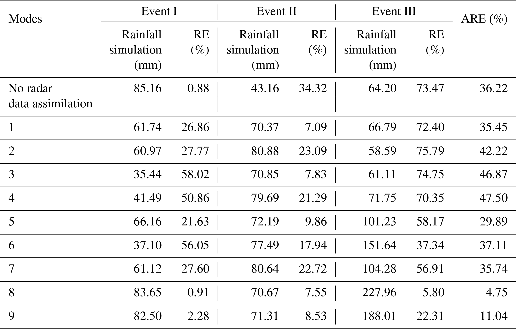
5.1.1 Evaluation of assimilating effects for the different kinds of radar data
The assimilating effects for three kinds of radar data are compared at different assimilating time intervals. Based on the REs of modes 1, 2, and 3, assimilating radar reflectivity always leads to better simulations than assimilating the other two kinds of radar data at a time interval of 6 h. The worst mode for event I is assimilating both radar reflectivity and radial velocity, while for events II and III, it is assimilating radial velocity. According to the REs of modes 4, 5, and 6, assimilating radial velocity becomes the best choice at a time interval of 3 h for the three storm events. Assimilating radar reflectivity has the worst performance in the three modes for events II and III, whereas assimilating radar reflectivity and radial velocity together has the worst performance for event I. When the time interval of data assimilation becomes 1 h, the ranking of assimilation modes for accumulated rainfall simulations is assimilating radial velocity>assimilating radar reflectivity and radial velocity>assimilating radar reflectivity.
5.1.2 Evaluation of assimilation effects for the different assimilation time intervals
The influences of assimilating time intervals on rainfall simulations are analyzed in this section. Comparing the REs of modes 1, 4, and 7, shortening the time interval of radar reflectivity assimilation has no obvious improvement for rainfall simulations and even makes the rainfall simulations worse. For assimilating radial velocity, all the rainfall simulations of the three storm events become more accurate, and the assimilation effects are significantly improved as the time interval shortens from 6 to 1 h. The REs of the three storm events are all lower than 8 % for the radial velocity assimilation at a time interval of 1 h. According to modes 3, 6, and 9, shortening the assimilation time interval can improve the rainfall simulations in most cases for assimilating radar reflectivity and radial velocity at the same time, while only the RE of mode 6 is higher than the RE of mode 3.
5.2 Spatiotemporal distribution of rainfall simulations based on the nine data assimilation modes
The spatiotemporal patterns of the rainfall have a significant effect on flood peak and peak time in medium and small catchments. The indices of CSI and RMSE are also applied to compare the nine radar data assimilation modes. The average CSI values and the average RMSE values for the three storm events are also calculated for different modes.
5.2.1 Evaluation in the spatial dimension
Table 6 indicates that although mode 8 with the highest CSI and lowest RMSE is the best choice in the nine data assimilation modes, rainfall simulations with data assimilation are always worse than without data assimilation for event I. Figure 4 shows that the observed rainfall center is located in the east of Meixi catchment, and it rains more in the upstream side than the downstream side. However, the spatial distribution of the accumulated 24 h rainfall with no data assimilation is even. Modes 1 and 2 simulate the rainfall on the east side of Meixi catchment accurately, while the simulated rainfall on the west side is much smaller than the observation. The rainfall simulations of modes 3, 4, 5, and 6 are all even in spatial dimension and lower than the observation. The simulation of mode 7 shows that the rainfall in the downstream side is less than the upstream side, whereas the different distribution in a east–west direction is not obvious, and the simulated rainfall is smaller than the observation. For mode 9, the spatial distribution of rainfall is also inconsistent with the observation. Only the simulation of mode 8 is close to the observed rainfall.
Table 6CSIs and RMSEs for the spatial distribution of rainfall simulations based on the nine data assimilation modes.
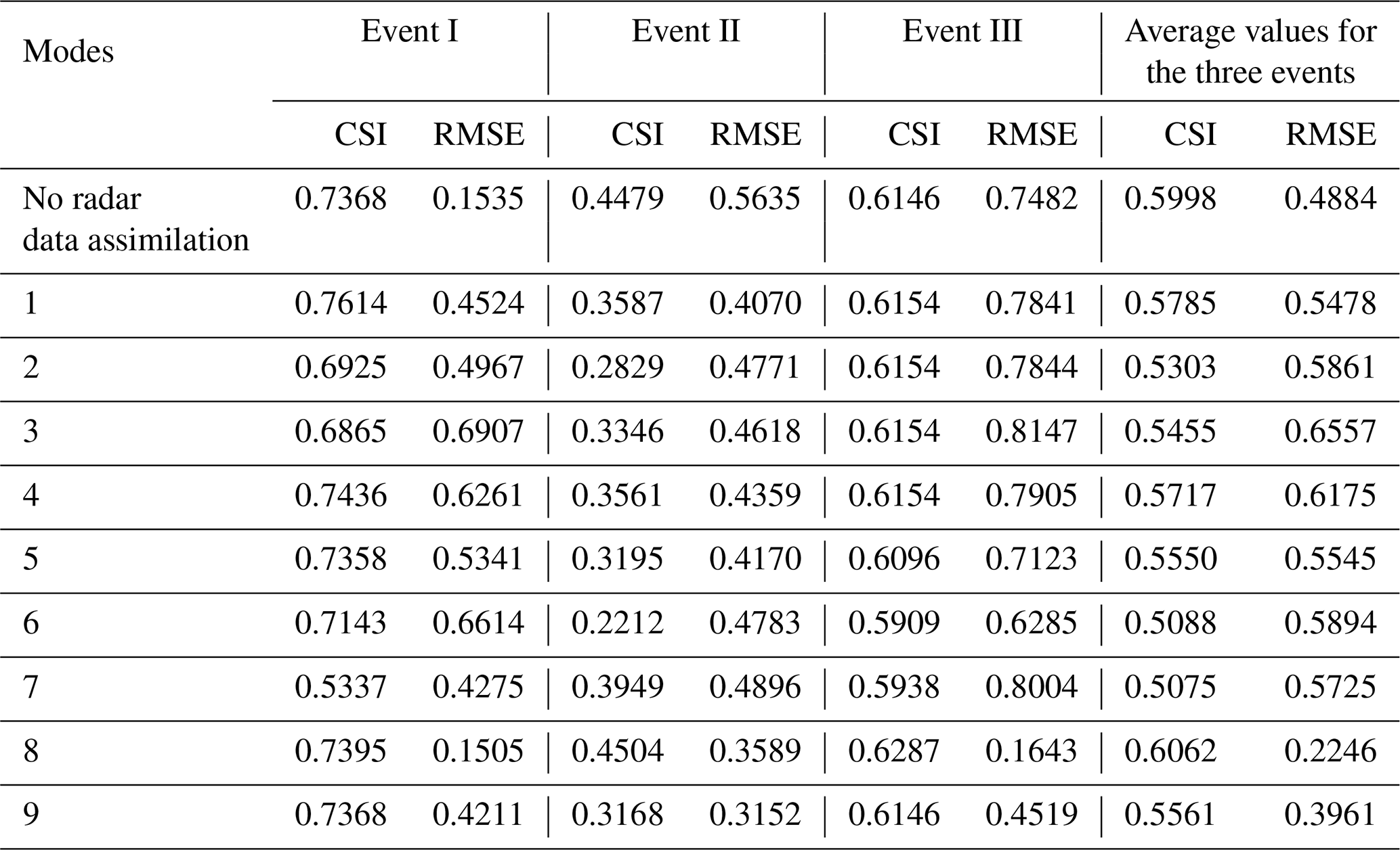
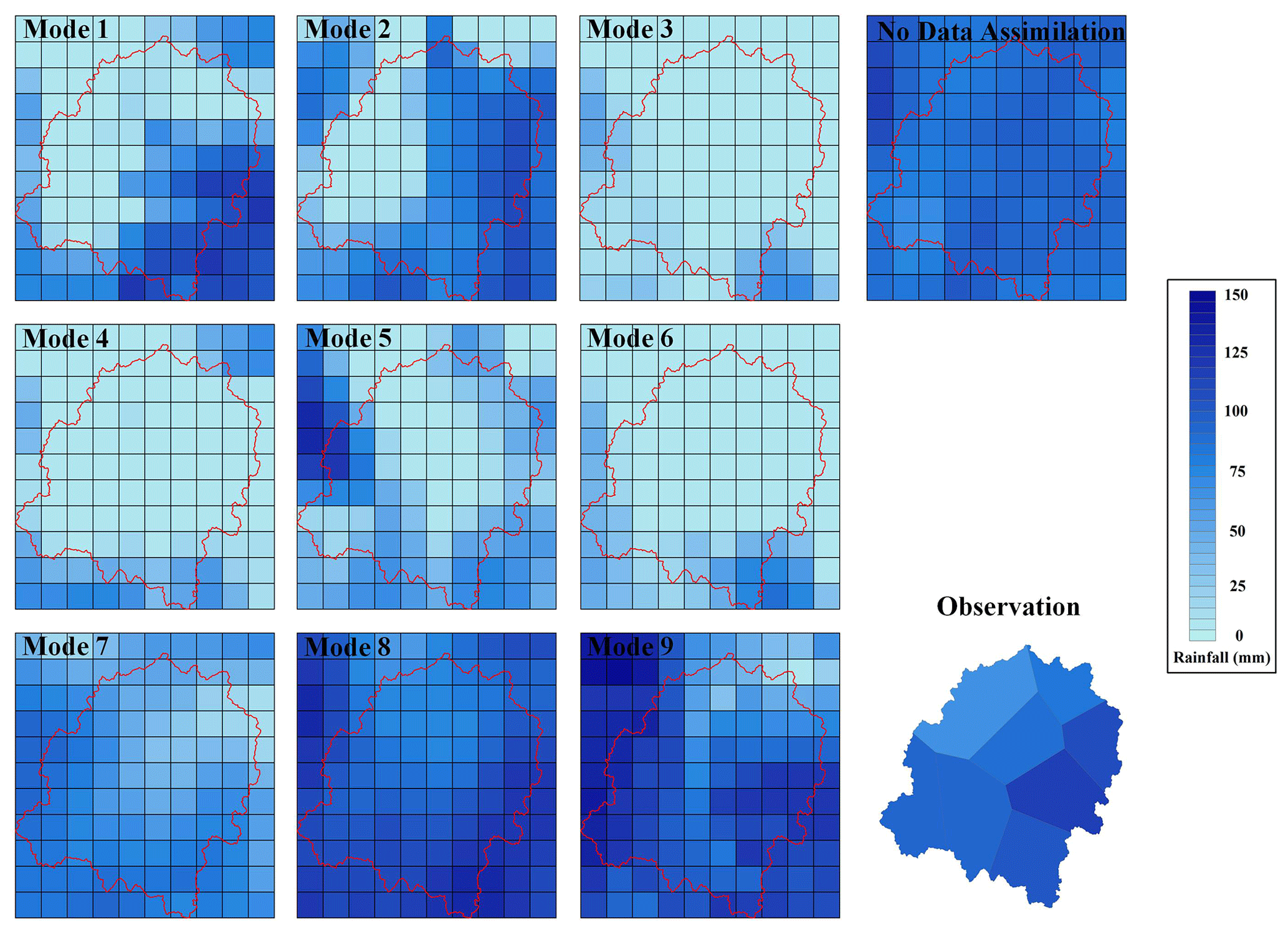
Figure 4Spatial distribution of the simulated 24 h rainfall accumulations with nine data assimilation modes for event I.
All RMSEs of the simulations with radar data assimilation are lower than without data assimilation, and only the CSI of mode 8 is higher than the simulation without data assimilation for event II. According to the rainfall distribution shown in Fig. 5, the falling areas of simulated rainfall without data assimilation are totally wrong. The observed rainfall center is located in the middle of the upstream and downstream catchment. However, the rainfall centers of modes 1, 4, and 7 are all located in the middle and lower region. The rainfall center is in the middle reaches for mode 2, while it is in the western catchment for mode 3. For modes 5 and 6, the spatial distributions of rainfall are also inconsistent with the observation. The simulated rainfall in the middle of the upstream catchment is close to the observation for modes 8 and 9 but in the downstream catchment is poor. Although the spatial rainfall distributions have deviations, nine modes get better than the simulations without data assimilation as a whole.
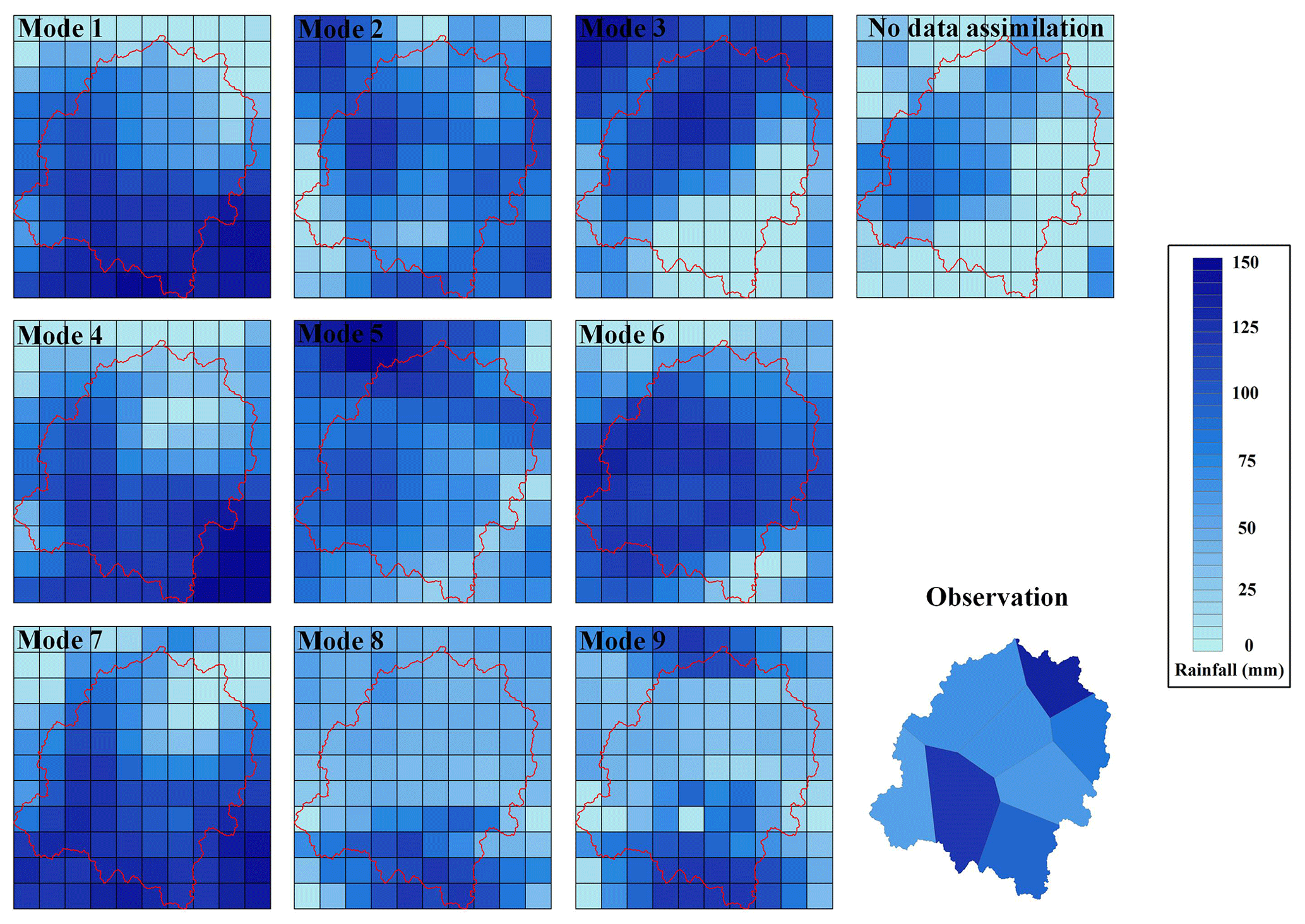
Figure 5Spatial distribution of the simulated 24 h rainfall accumulations with nine data assimilation modes for event II.
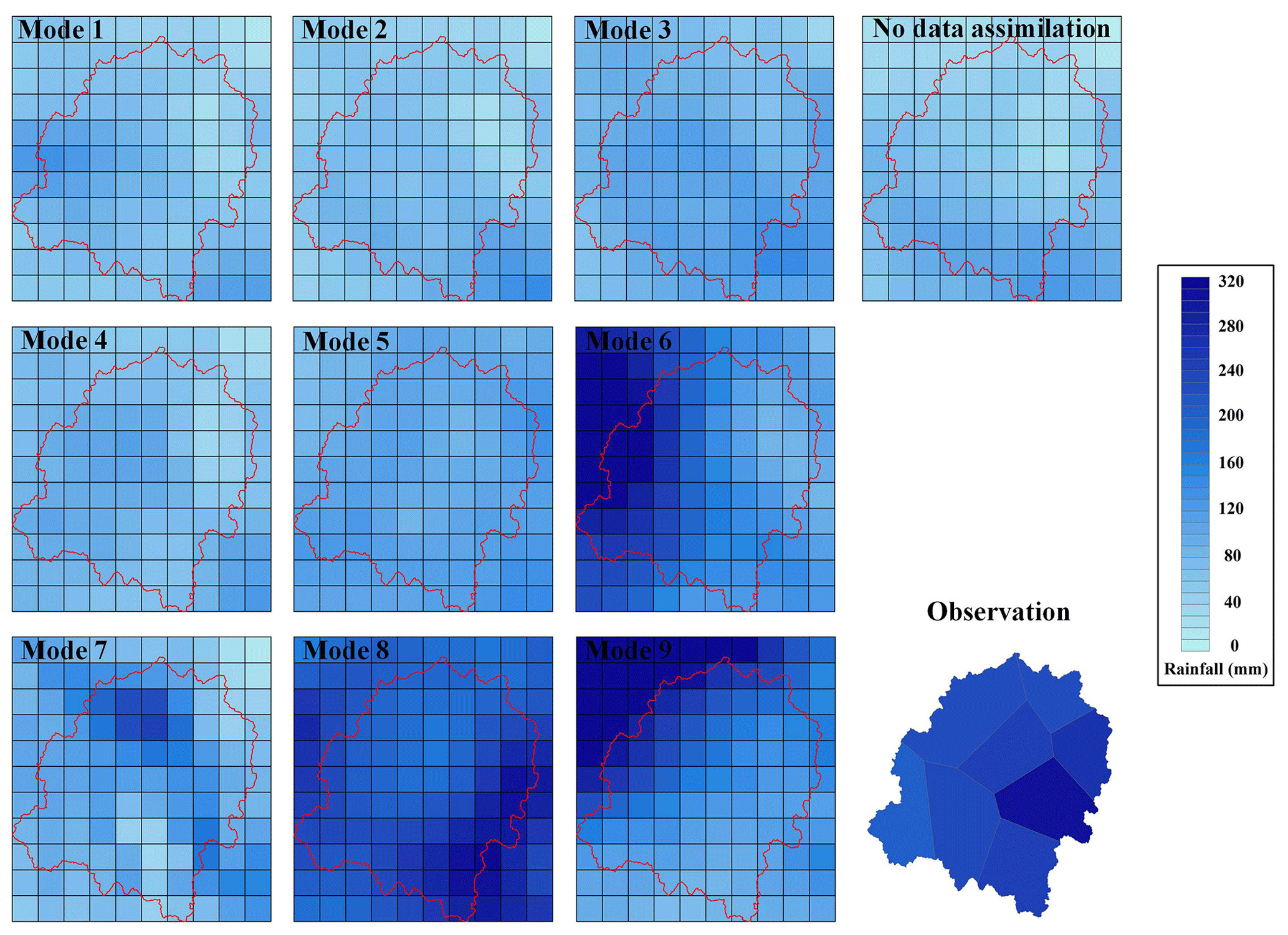
Figure 6Spatial distribution of the simulated 24 h rainfall accumulations with nine data assimilation modes for event III.
Based on Table 6, not all data assimilation modes help improve the rainfall simulations for event III. Modes 4, 5, and 9 have just a little improvement on rainfall simulations in spatial distribution, and only the simulation of mode 8 is close to the observation. The simulations of modes 1, 2, 3, 4, and 5 are much lower than the observation in the whole catchment. Most observed rainfall falls in the east of the catchment, while the simulated rainfall concentrates in the west for modes 6 and 9 and in the downstream catchment for mode 7.
Based on the CSIs and RMSEs of modes 1, 2, and 3, assimilating radar reflectivity performs better than assimilating the other two kinds of radar data at a time interval of 6 h. Assimilating radar reflectivity and radial velocity at the same time always leads to the worst simulations. Comparing the two indices of modes 4, 5, and 6, assimilating radar reflectivity at a time interval of 3 h can obtain the highest CSI for the three storm events, while assimilating radial velocity has a better performance than the other two modes based on RMSE for events I and II. For the time interval of 1 h, the ranking of assimilation modes for the spatial distribution of rainfall simulations is assimilating radial velocity>assimilating radar reflectivity and radial velocity>assimilating radar reflectivity.
Table 7CSIs and RMSEs for the temporal distribution of rainfall simulations based on the nine data assimilation modes.
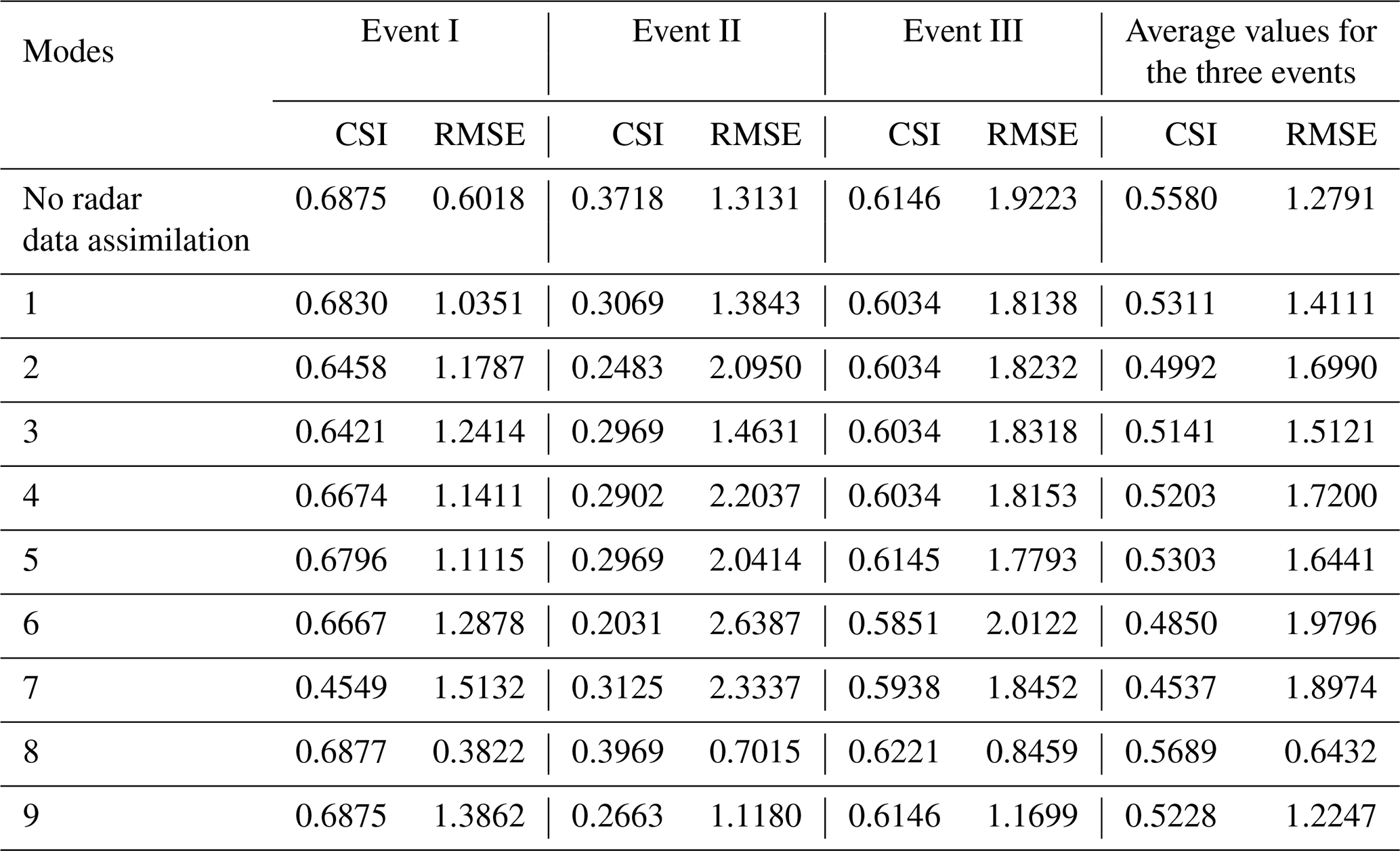
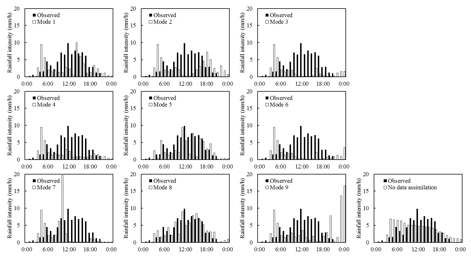
Figure 7Time series bars of observed and simulated areal rainfall with nine data assimilation modes and the rainfall observation for event I.
Comparing the two indices of modes 1, 4, and 7, rainfall simulations become even worse as the time interval of radar reflectivity assimilation shortens. For the three modes of assimilating radial velocity, most simulations become more accurate, and the assimilation effects are significantly improved as the time interval shortens from 6 to 1 h. The same conclusion can be obtained for assimilating radar reflectivity and radial velocity at the same time, while the improvement is not as obvious as assimilating radial velocity.
5.2.2 Evaluation in the temporal dimension
As shown in Table 7, similar results can be found that most data assimilation modes cannot help the simulations of the WRF model get better for event I. Only mode 8 is outstanding with the highest CSI and lowest RMSE. Figure 7 shows that the rainfall is concentrated at 10:00–16:00 for the observation. However, the main rainfall processes occur at 03:00–05:00 for modes 3, 4, and 6, 03:00–05:00 and 14:00–15:00 for mode 1, 03:00–05:00 and 17:00–19:00 for mode 2, 03:00–05:00 and 09:00–10:00 for mode 7, and 03:00–05:00 and 20:00–24:00 for mode 9. The rainfall processes of modes 5 and 8 are similar with the observation, while the rainfall simulations at 12:00–13:00 and 15:00 for mode 5 are worse than for mode 8.
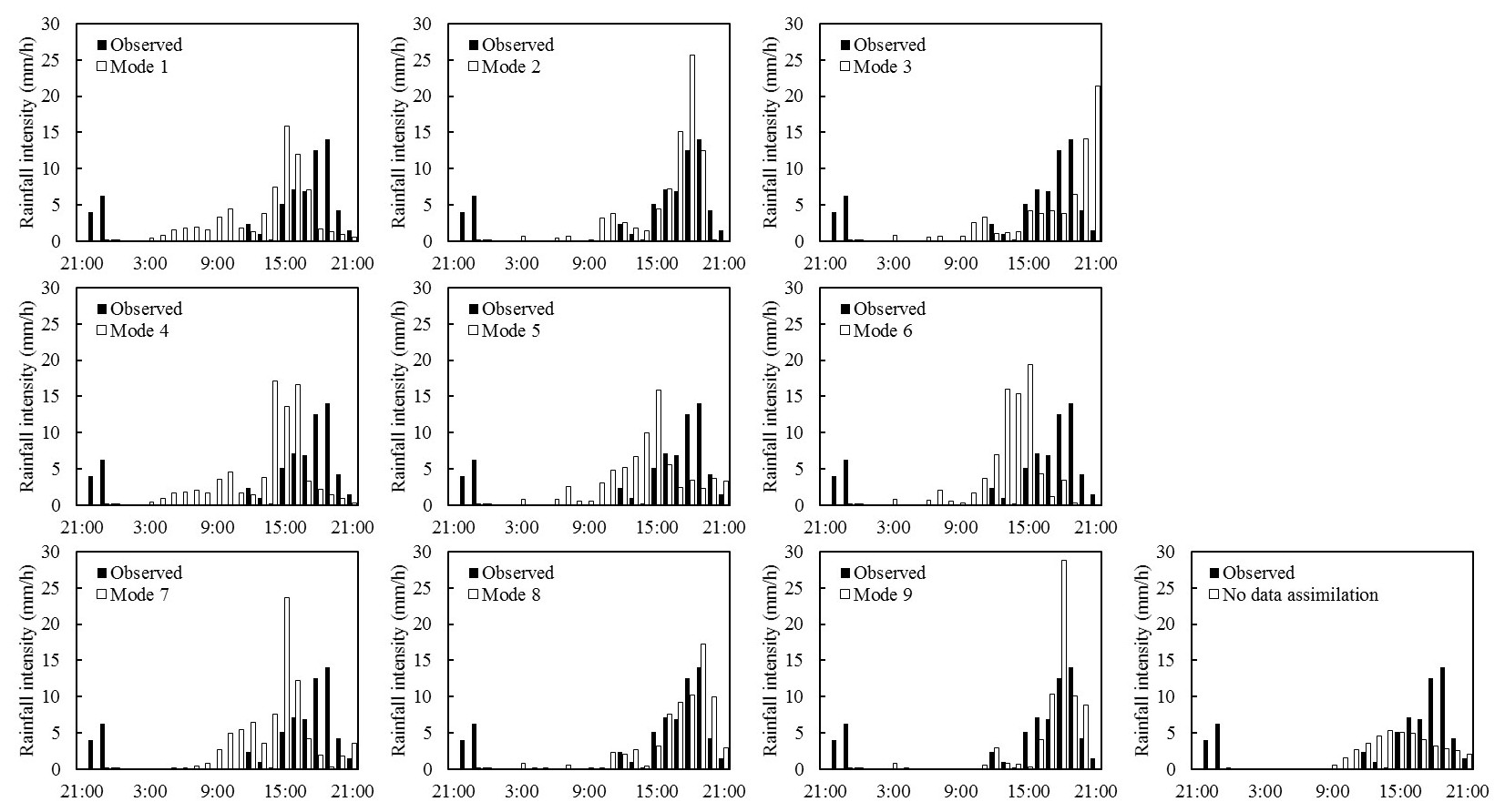
Figure 8Time series bars of observed and simulated areal rainfall with nine data assimilation modes and the rainfall observation for event II.
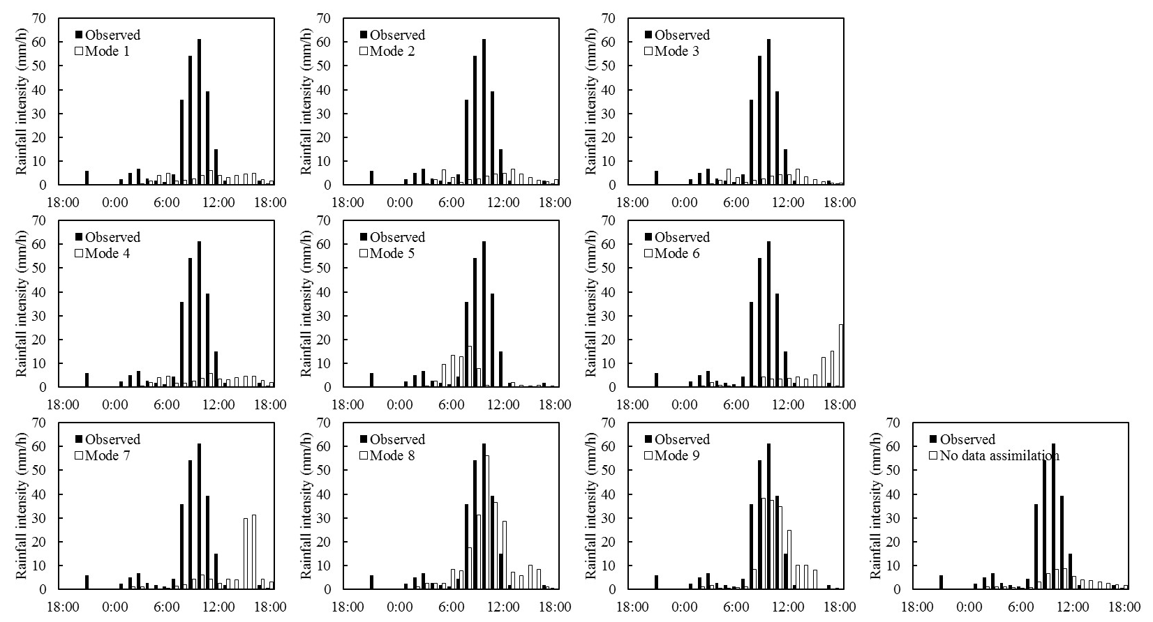
Figure 9Time series bars of observed and simulated areal rainfall with nine data assimilation modes and the rainfall observation for event III.
According to the values of CSI and RMSE, only modes 8 and 9 are useful for the improvement of rainfall simulations, and obvious improvement can be found in mode 8 for event II. The actual main rainfall process occurs at 15:00–18:00, while the time is advanced by 3 h for modes 1, 4, 5, 6, and 7. There is a delay of 3 h for the main rainfall process of mode 3. Although the times of heavy rainfall for modes 2 and 9 are consistent with the observation, the areal rainfall at 18:00 is much higher than the observation.
For event III, although most CSIs of the simulations with radar data assimilation are lower than the simulations without data assimilation, the RMSEs show the opposite conclusions. From Fig. 9, the observed rainfall is concentrated at 08:00–11:00. It can be easily found that modes 1, 2, 3, 4, 5, and 6 cannot reproduce the heavy rainfall process in temporal dimension. The simulated rainfall is concentrated at 15:00–16:00 for mode 7. Only the simulation of mode 8 is basically consistent with the observation, while the simulation of mode 9 is worse than mode 8 at 08:00 and 10:00.
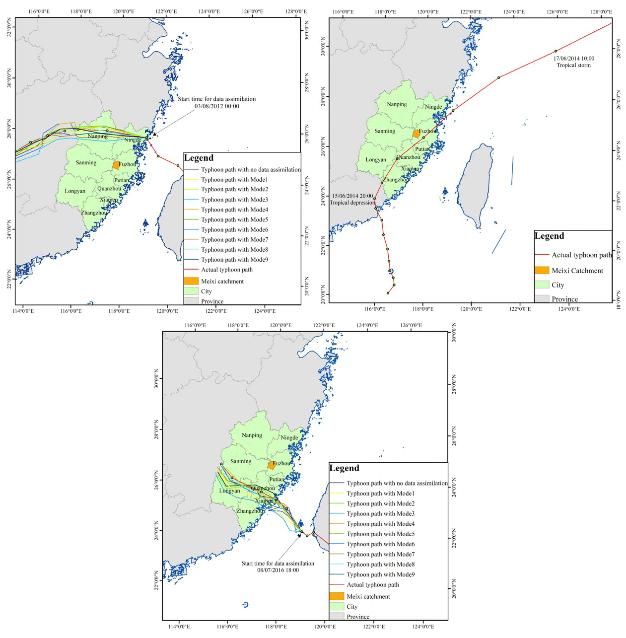
Figure 10Typhoon path and simulations for (a) Saola, (b) Hagibis, and (c) Nepartak.
According to the CSIs and RMSEs of modes 1, 2, and 3, assimilating radar reflectivity at a time interval of 6 h performs better than assimilating the other two kinds of radar data. Assimilating radial velocity performs the worst for event II, and assimilating radar reflectivity and radial velocity at the same time always leads to the worst simulations for events I and III. Based on the two indices of modes 4, 5, and 6, assimilating radial velocity at a time interval of 3 h can obtain the highest CSI and lowest RMSE for the three storm events, while assimilating radar reflectivity and radial velocity at the same time performs worse than the other two modes. For the time interval of 1 h, the ranking of assimilation modes for the temporal distribution of rainfall simulations is assimilating radial velocity>assimilating radar reflectivity and radial velocity>assimilating radar reflectivity.
Comparing the indices of modes 1, 4 and 7, rainfall simulations for temporal distribution become even worse as the time interval of radar reflectivity assimilation shortens from 6 to 1 h. For modes 2, 5, and 8, shortening the time interval can significantly improve the rainfall simulations by assimilating radial velocity. Modes 3, 6, and 9 indicate that rainfall simulations are improved by shortening the time interval as a whole, whereas assimilating radar reflectivity and radial velocity at the same time at a time interval of 3 h obtains the worst rainfall simulations for events II and III.
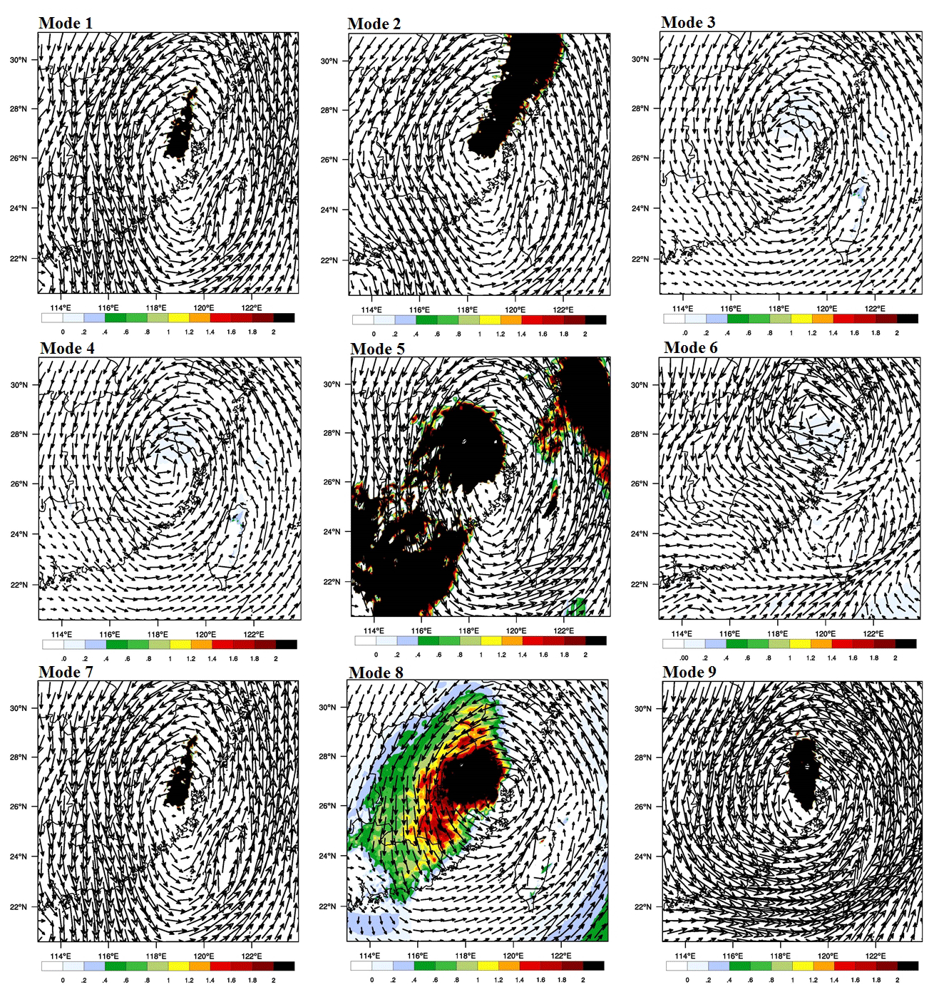
Figure 11Water vapor transportation increment and wind field (850 hPa) for event I at 12:00 on 3 August 2012.
In order to prove the accuracy of the assimilation results, typhoon paths for different assimilation modes are also simulated (Fig. 10). According to the simulations of Saola and Nepartak, the accurate typhoon path simulations always lead to accurate rainfall simulations. However, for typhoon Hagibis, the actual typhoon center is far away from the Meixi catchment during the assimilation process. Hence, only the actual typhoon path for Hagibis is added in Fig. 10. Comparing the nine radar data assimilation modes, assimilating radial velocity at a time interval of 6 h always performs the worst in rainfall simulations, while the rainfall simulations can be significantly improved by shortening the time interval of data assimilation. According to Eq. (3), although the physical process of the rainfall formation cannot be influenced by the radial velocity assimilation directly, the wind field and the water vapor transportation in initial and lateral boundary conditions can be changed with the wind information in radial velocity. However, the wind field is quite variable, especially for stormy weather. As the time interval becomes longer, the WRF model cannot be corrected by the radial velocity in time, whereas compared to the simulations without data assimilation, the inevitable observation errors caused by atmospheric refractivity in the radial velocity might lead to worse performance in the WRF model as the running time goes on (Montmerle and Faccani, 2009). That is the main reason that assimilating radial velocity at a time interval of 6 h cannot obtain satisfactory simulations. Increasing the frequency of data assimilation, the effective information in radial velocity can correct the wind field and the water vapor transportation in the background field of the WRF model timely, which is helpful to improve the rainfall simulations (Kawabata et al., 2014).
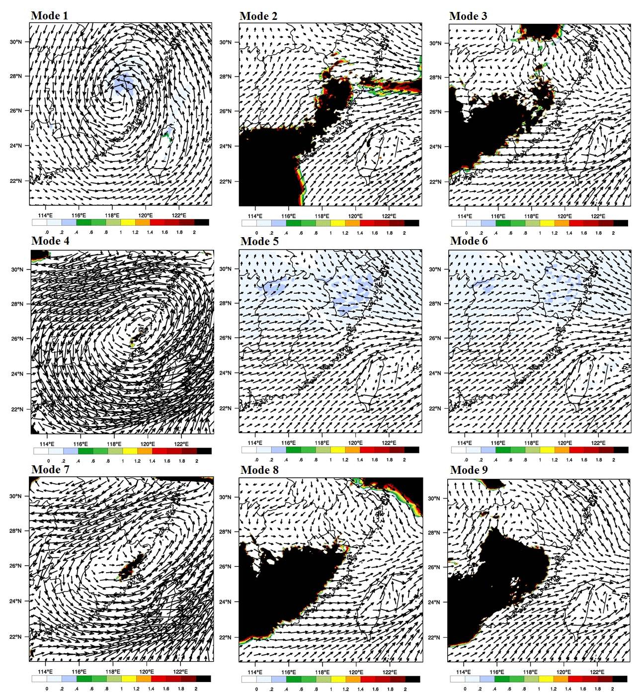
Figure 12Wind field and water vapor transportation increment (850 hPa) for event II at 18:00 on 18 June 2014.
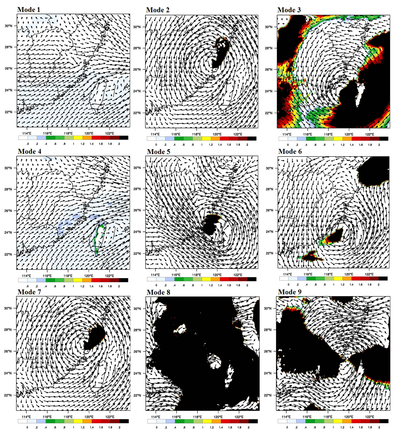
Figure 13Wind field and water vapor transportation increment (850 hPa) for event III at 06:00 on 9 July 2016.
The water vapor transportation increments and wind field for different modes at the rainfall concentrating time are used to show how assimilating radial velocity and radar reflectivity affects the WRF model's initial and boundary conditions (Figs. 11–13). The shadows in Figs. 11–13 mean that water vapor transportation in the analysis field is more than in the background field. The darker the shadow in the figures is, the more the water vapor transportation increment is, which is one of the most important factors that affects the amount of rainfall. For event I, counterclockwise wind field has contributed to the water vapor transportation from ocean to inland at 12:00 on 3 August 2012. Modes 1, 2, 5, 7, 8, and 9 all obtain the shadow area with the obvious water vapor transportation increment. However, according to the coverage area of the shadow, only modes 5 and 8 influence Meixi catchment directly, which is consistent with the result that rainfall simulations with modes 5 and 8 are higher than simulations with no data assimilation at 12:00, while the increment of simulated rainfall is quite obvious for mode 8. The differences of nine modes can be easily found in both the wind field and water vapor transportation increments for event II. The water vapor transportation increases significantly in modes 2, 3, 8, and 9 at 18:00 on 18 June 2014, which has a direct impact on the rainfall simulations in Meixi catchment. That is the main reason why simulated rainfalls with modes 2, 3, 8, and 9 are higher than the simulated rainfall with no data assimilation. However, the wind fields in these modes indicate a lack of warm and wet flow supply, and the rainfall weakening is almost inevitable after 18:00. Considering the wind field and the range of water vapor transportation increments, the rainfalls may continue for a period of time after 18:00 in modes 3, 8, and 9, which can also be reflected by hourly simulated rainfall shown in Fig. 8. For event III, the water vapor transportation increases significantly in modes 2, 3, 5, 6, 7, 8, and 9 at 06:00 on 9 July 2016, while only modes 8 and 9 affect Meixi catchment directly. The range of shadows in Fig. 13 is also consistent with the rainfall simulations. The wind field indicates that water vapor transportation is sufficient for mode 8 at a later time, which leads to a significant increase in simulated rainfall.
Does further shortening the assimilation interval obtain better rainfall simulations? In terms of theory, the answer is yes because improving the assimilation frequency can correct the initial and lateral boundary conditions in a timely manner. However, the observation errors of radial velocity may be amplified with the high assimilation frequency in the WRF model. There may be an “inverted u” relationship between the accuracy of the rainfall simulations and the assimilation time interval (Myung et al., 2000). Further study should be carried out to investigate the optimal assimilation time interval.
On the contrary, assimilating radar reflectivity offers little help for improving rainfall simulations except for accumulated rainfall. Furthermore, rainfall simulations become even worse as the time interval of radar reflectivity assimilation shortens from 6 to 1 h. The background field of the WRF model has large differences from the actual weather situation, which can be reflected in the rainfall simulations without data assimilation against the rainfall observations for the three storm events. As shown in Eq. (2), radar reflectivity is closely related to the humidity field and contains the information of rainfall hydrometeors (Wattrelot et al., 2014). That is to say the humidity information in radar reflectivity is quite different from the actual weather situation, which makes it difficult for the 3-DVar data assimilation to produce an optimal estimate of the true atmospheric state by the iterative solution of a prescribed cost function. It should also be mentioned that due to its unchangeability, the matrix of CV3 has wide applicability but is not practical for all cases (Kong et al., 2017). The inadaptability of CV3 in the typhoon synoptic system and the large differences between the humidity information in radar reflectivity and the actual weather situation might be the main reasons for the poor performance of radar reflectivity assimilation (Sun, 2005). The more frequent the radar reflectivity assimilation is, the greater the pressure on the 3-DVar data assimilation model is. Other data assimilation models with variable background error covariance, such as the hybrid ensemble transform Kalman filter–three-dimensional variational data assimilation (ETKF-3DVAR) (Wang et al., 2012; Shen et al., 2016), should be tested for radar reflectivity assimilation in future studies.
For the even rainfall events in space and time, such as storm event I, data assimilation should be used carefully. The WRF model has good performance in rainfall simulations, especially for accumulated rainfall. The errors in the assimilated data may have a negative effect on the rainfall simulations. Additionally, assimilating other kinds of data and radar data together may help to improve the rainfall simulations. Though the conventional observations, such as upper-air and surface observations from meteorological stations and sounding balloons, have low spatiotemporal resolution, the kinds of data are various and have wide coverage, which can help to improve the atmospheric motion in the WRF model at large scales (Li et al., 2018). Yesubabu et al. (2016) indicate that assimilating the satellite observation also has a positive effect on the rainfall simulations. Assimilating different data sources, together with the radar data, may further improve the rainfall simulations at catchment scale. In reality, ECMWF was also tested for the data assimilation before FNL was used in this study (Zhang et al., 2018; Zhao et al., 2012). Although the rainfall simulations show some differences based on the two kinds of boundary conditions, the patterns of improvements from different data assimilation modes are quite similar, and the same conclusions can be obtained.
Data assimilation is an efficient technique for improving rainfall simulations. In order to explore the reasonable use of Doppler radar data assimilation to correct the initial and lateral boundary conditions of the NWP systems, three typhoon storm events, including Saola, Hagibis, and Nepartak, are chosen to be simulated by the WRF model with nine modes in Meixi catchment located on the southeast coast of China. The FNL analysis data with grids are used to drive the WRF model, and radar data from the Changle Doppler radar station are applied to correct the initial and lateral boundary conditions. Three evaluating indices, RE, CSI, and RMSE, are used to evaluate the nine radar data assimilation modes, which are designed by three kinds of radar data (radar reflectivity, radial velocity, and radar reflectivity and radial velocity) and at three assimilation time intervals (1, 3, and 6 h).
Contrastive analyses of the nine modes are carried out from three aspects: accumulated rainfall simulations, spatial rainfall distribution, and temporal rainfall distribution. Four main conclusions are obtained: (1) in the nine radar data assimilation modes, assimilating radial velocity at a time interval of 1 h can significantly improve the rainfall simulations and outperform the other modes for all the three storm events; (2) shortening the assimilation time interval can improve the rainfall simulations in most cases, while assimilating radar reflectivity always leads to worse simulations as the time interval shortens; (3) radar reflectivity is the best choice for the data assimilation at a time interval of 6 h, while radial velocity performs best for the data assimilation at a time interval of 1 h; and (4) data assimilation can improve the rainfall simulations as a whole, especially for the heavy rainfall with strong convection, whereas the improvement for evenly distributed rainfall in space and time is limited. More numerical simulation experiments should be tested in other catchments in different climate conditions. Further studies also should be carried out to investigate the data assimilation techniques to improve the ability of the simulations of heavy rainfall in the study areas.
The rainfall data from gauges used in this study were provided by the Fujian Institute of Water Resources and Hydropower. The radar data were provided by the newest-generation weather radar network of China (CINRAD/SC). The NCEP Final (FNL) Operational Global Analysis data are available at https://rda.ucar.edu/datasets/ds083.2/ (NCAR, 2020).
All the authors contributed to the conception and the development of this paper. JT and RL contributed to radar data assimilation and paper writing. LD and LG assisted in the design and analyses of the data assimilation modes. BZ helped with the figure production.
The authors declare that they have no conflict of interest.
We thank the NHESS editor and two reviewers for constructive comments which improved the study.
This research has been supported by the National Key R&D Program (grant nos. 2019YFC1510605 and 2018YFC1508105), the National Natural Science Foundation of China (grant nos. 51909274 and 51822906), and the IWHR Research & Development Support Program (grant nos. JZ0145B032020 and WR0145B732017).
This paper was edited by Vassiliki Kotroni and reviewed by two anonymous referees.
Agnihotri, G. and Dimri, A. P.: Simulation study of heavy rainfall episodes over the southern Indian peninsula, Meteorol. Appl., 22, 223–235, https://doi.org/10.1002/met.1446, 2015.
Avolio, E. and Federico, S.: WRF simulations for a heavy rainfall event in southern Italy: Verification and sensitivity tests, Atmos. Res., 209, 14–35, https://doi.org/10.1016/j.atmosres.2018.03.009, 2018.
Bauer, H. S., Schwitalla, T., Wulfmeyer V., Bakhshaii, A., Ehret, U., Neuper, M., and Caumont, O: Quantitative precipitation estimation based on high-resolution numerical weather prediction and data assimilation with WRF – a performance test, Tellus A., 67, 25047, https://doi.org/10.3402/tellusa.v67.25047, 2015.
Cai, Y., Lu, X., Chen, G., and Yang, S: Diurnal cycles of Mei-yu rainfall simulated over eastern China: Sensitivity to cumulus convective parameterization, Atmos. Res., 213, 236–251, https://doi.org/10.1016/j.atmosres.2018.06.003, 2018.
Caya, A., Sun, J., and Snyder, C.: A comparison between the 4DVAR and the Ensemble Kalman Filter techniques for radar data assimilation, Mon. Weather Rev., 133, 3081–3094, https://doi.org/10.1175/MWR3021.1, 2005.
Chen, X., Wang, Y., Zhao, K., and Wu, D: A numerical study on rapid intensification of typhoon Vicente (2012) in the South China Sea. Part I: verification of simulation, storm-scale evolution, and environmental contribution, Mon. Weather Rev., 145, 877–898, https://doi.org/10.1175/MWR-D-16-0147.1, 2017.
Dai, Q., Yang, Q., Han, D., Rico-Ramirez, M. A., and Zhang, S: Adjustment of radar-gauge rainfall discrepancy due to raindrop drift and evaporation using the Weather Research and Forecasting model and dual-polarization radar, Water Resour. Res., 55, 9211–9233, https://doi.org/10.1029/2019WR025517, 2019.
Giannaros, T. M., Kotroni, V., and Lagouvardos, K.: WRF-LTNGDA: A lightning data assimilation technique implemented in the WRF model for improving precipitation forecasts, Environ. Model. Softw., 76, 54–68, https://doi.org/10.1016/j.envsoft.2015.11.017, 2016.
Hazra, A., Chaudhari, H. S., Ranalkar, M., and Chen, J. P: Role of interactions between cloud microphysics, dynamics and aerosol in the heavy rainfall event of June 2013 over Uttarakhand, India, Q. J. Roy. Meteor. Soc., 143, 986–998, https://doi.org/10.1002/qj.2983, 2017.
Hou, T., Kong, F., Chen, X., Lei, H., and Hu, Z: Evaluation of radar and automatic weather station data assimilation for a heavy rainfall event in southern China, Adv. Atmos. Sci., 32, 967–978, https://doi.org/10.1007/s00376-014-4155-7, 2015.
Ide, K., Courtier, P., Ghil, M., and Lorenc, A. C: Unified Notation for data assimilation: Operational, sequential and variational, J. Meteorol. Soc. Jpn., 75, 181–189, https://doi.org/10.1175/1520-0469(1997)054<0679:OTRBTS>2.0.CO;2, 1997.
Kawabata, T., Iwai, H., Seko, H., Shoji, Y., Saito, K., Ishii, S., and Mizutani, K: Cloud-resolving 4D-Var assimilation of Doppler wind lidar data on a Meso-Gamma-Scale convective system, Mon. Weather Rev., 142, 4484–4498, https://doi.org/10.1175/MWR-D-13-00362.1, 2014.
Kong, R., Xue, M., and Liu, C. Development of a hybrid En3DVar data assimilation system and comparisons with 3DVar and EnKF for radar data assimilation with observing system simulation experiments, Mon. Weather Rev., 146, 175–198, https://doi.org/10.1175/MWR-D-17-0164.1, 2017.
Li, X., Fan, K., and Yu, E.: Hindcast of extreme rainfall with high-resolution WRF: model ability and effect of physical schemes, Theor. Appl. Climatol., 139, 639–658, https://doi.org/10.1007/s00704-019-02945-2, 2019.
Li, Z., Ballard, S. P., and Simonin, D.: Comparison of 3D-Var and 4D-Var data assimilation in an NWP-based system for precipitation nowcasting at the Met Office, Q. J. Roy. Meteor. Soc., 144, 404–413, https://doi.org/10.1002/qj.3211, 2018.
Liu, J., Bray M., and Han, D.: Sensitivity of the Weather Research and Forecasting (WRF) model to downscaling ratios and storm types in rainfall simulation, Hydrol. Process., 26, 3012–3031, https://doi.org/10.1002/hyp.8247, 2012.
Liu, J., Bray, M., and Han D.: Exploring the effect of data assimilation by WRF-3DVar for numerical rainfall prediction with different types of storm events, Hydrol. Process., 27, 3627–3640, https://doi.org/10.1002/hyp.9488, 2013.
Liu, J., Tian, J., Yan, D., Li, C., Yu, F., and Shen, F.: Evaluation of Doppler radar and GTS data assimilation for NWP rainfall prediction of an extreme summer storm in northern China: from the hydrological perspective, Hydrol. Earth Syst. Sci., 22, 4329–4348, https://doi.org/10.5194/hess-22-4329-2018, 2018.
Lu, X., Wang X., Li Y., Tong, M., and Ma, X: GSI-based ensemble-variational hybrid data assimilation for HWRF for hurricane initialization and prediction: impact of various error covariances for airborne radar observation assimilation, Q. J. Roy. Meteor. Soc., 143, 223–239, https://doi.org/10.1002/qj.2914, 2017.
Maiello, I., Ferretti, R., Gentile, S., Montopoli, M., Picciotti, E., Marzano, F. S., and Faccani, C.: Impact of radar data assimilation for the simulation of a heavy rainfall case in central Italy using WRF–3DVAR, Atmos. Meas. Tech., 7, 2919–2935, https://doi.org/10.5194/amt-7-2919-2014, 2014.
Meng, Z. and Zhang, F.: Tests of an ensemble Kalman filter for mesoscale and regional-scale data assimilation. Part III: Comparison with 3DVAR in a real-data case study, Mon. Weather Rev., 136, 522–540, https://doi.org/10.1175/mwr3352.1, 2008.
Milan, M., Venema, V., Schüttemeyer, D., and Simmer, C: Assimilation of radar and satellite data in mesoscale models: A physical initialization scheme, Meteorol. Z., 17, 887–902, https://doi.org/10.1127/0941-2948/2008/0340, 2008.
Mohan, G. M., Srinivas, C. V., and Naidu, C. V.: Real-time numerical simulation of tropical cyclone Nilam with WRF: experiments with different initial conditions, 3D-Var and Ocean Mixed Layer Model, Nat. Hazards., 77, 597–624, https://doi.org/10.1007/s11069-015-1611-3, 2015.
Montmerle, T. and Faccani, C.: Mesoscale assimilation of radial velocities from Doppler radars in a preoperational framework, Mon. Weather Rev., 137, 1939–1953, https://doi.org/10.1175/2008MWR2725.1, 2009.
Myung, J. I.: The importance of complexity in model selection, J. Math. Psychol., 44, 190–204, https://doi.org/10.1006/jmps.1999.1283, 2009.
NCAR: NCEP Final (FNL) Operational Global Analysis data, available at: https://rda.ucar.edu/datasets/ds083.2/, last access: 10 January 2020.
Otieno, G., Mutemi, J. N., Opijah, F. J., Ogallo, L. A., and Omondi, M. H: The sensitivity of rainfall characteristics to cumulus parameterisation schemes from a WRF model. Part I: a case study over East Africa during wet years, Pure Appl. Geophys., 1, 1–16, https://doi.org/10.1007/s00024-019-02293-2, 2019.
Prakash, S., Sathiyamoorthy, V., Mahesh, C., and Gairola, R. M: An evaluation of high-resolution multisatellite rainfall products over the Indian monsoon region, Int. J. Remote Sens., 35, 3018–3035, https://doi.org/10.1080/01431161.2014.894661, 2014.
Shen, F., Min, J., and Xu, D.: Assimilation of radar radial velocity data with the WRF Hybrid ETKF-3DVAR system for the prediction of Hurricane Ike (2008), Atmos. Res., 169, 127–138, https://doi.org/10.1016/j.atmosres.2015.09.019, 2016.
Shen, F., Xue, M., and Min, J.: A comparison of limited-area 3DVAR and ETKF-En3DVAR data assimilation using radar observations at convective scale for the prediction of Typhoon Saomai (2006), Meteorol. Appl., 24, 628–641, https://doi.org/10.1002/met.1663, 2017.
Sivapalan, M. and Blöschl, G.: Transformation of point rainfall to areal rainfall: Intensity-duration-frequency curves, J. Hydrol., 204, 150–167, https://doi.org/10.1016/S0022-1694(97)00117-0, 1998.
Srivastava, P. K., Han, D., Rico-Ramirez, M. A., O'Neill, P., Islam, T., Gupta, M., and Dai, Q: Performance evaluation of WRF-Noah Land surface model estimated soil moisture for hydrological application: Synergistic evaluation using SMOS retrieved soil moisture, J. Hydrol., 529, 200–212, 2015.
Sun, J.: Convective-scale assimilation of radar data: progress and challenges, Q. J. Roy. Meteor. Soc., 131, 3439–3463, 2005.
Sun, J. and Crook, N. A.: Dynamical and microphysical retrieval from Doppler radar observations using a cloud model and its adjoint, Part I: model development and simulated data experiments, J. Atmos. Sci., 54, 1642–1661, https://doi.org/10.1175/1520-0469(1997)054<1642:DAMRFD>2.0.CO;2, 1997.
Sun, J. and Crook, N. A.: Dynamical and microphysical retrieval from Doppler radar observations using a cloud model and its adjoint. Part II: retrieval experiments of an observed Florida convective storm, J. Atmos. Sci., 55, 835–852, https://doi.org/10.1175/1520-0469(1998)0552.0.CO;2, 1998.
Tian, J., Liu, J., Wang, J., Li, C., Yu, F., and Chu, Z: A spatio-temporal evaluation of the WRF physical parameterisations for numerical rainfall simulation in semi-humid and semi-arid catchments of Northern China, Atmos. Res., 198, 132–144, https://doi.org/10.1016/j.atmosres.2017.03.012, 2017a.
Tian, J., Liu, J., Yan, D., Li, C., Chu, Z., and Yu, F: An assimilation test of Doppler radar reflectivity and radial velocity from different height layers in improving the WRF rainfall forecasts, Atmos. Res., 198, 132–144, https://doi.org/10.1016/j.atmosres.2017.08.004, 2017b.
Tian, J., Liu, J., Yan, D., Ding, L., and Li, C.: Ensemble flood forecasting based on a coupled atmospheric-hydrological modeling system with data assimilation, Atmos. Res., 224, 127–137, https://doi.org/10.1016/j.atmosres.2019.03.029, 2019.
Tian, J., Liu, R., Ding, L., Guo, L., and Liu, Q.: Evaluation of the WRF physical parameterisations for Typhoon rainstorm simulation in southeast coast of China, Atmos. Res., 247, 105130, https://doi.org/10.1016/j.atmosres.2020.105130, 2021.
Wan, Q. and Xu, J.: A numerical study of the rainstorm characteristics of the June 2005 flash flood with WRF/GSI data assimilation system over south-east China, Hydrol. Process., 25, 1327–1341, https://doi.org/10.1002/hyp.7882, 2011.
Wang, H., Sun, J., Zhang, X., Huang, X. Y., and Auligné, T: Radar data assimilation with WRF 4D-Var. Part I: System development and preliminary testing, Mon. Weather Rev., 141, 2224–2244, https://doi.org/10.1175/MWR-D-12-00168.1, 2013.
Wang, X., Barker, D. M., Snyder, C., and Hamill, T. M: A hybrid ETKF–3DVAR data assimilation scheme for the WRF model. Part II: real observation experiments, Mon. Weather Rev., 136, 5132–5147, https://doi.org/10.1175/2008MWR2445.1, 2012.
Wattrelot, E., Caumont, O., and Mahfouf, J. F.: Operational implementation of the 1D+3D-Var assimilation method of radar reflectivity data in the AROME model, Mon. Weather Rev., 142, 1852–1873, https://doi.org/10.1175/mwr-d-13-00230.1, 2014.
Xie, Y., Xing, J., Shi, J., Dou, Y., and Lei, Y.: Impacts of radiance data assimilation on the Beijing 7.21 heavy rainfall, Atmos. Res., 169, 318–330, https://doi.org/10.1016/j.atmosres.2015.10.016, 2016.
Yesubabu, V., Srinivas, C. V., Langodan, S., and Hoteit, I.: Predicting extreme rainfall events over Jeddah, Saudi Arabia: impact of data assimilation with conventional and satellite observations, Q. J. Roy. Meteorol. Soc., 142, 327–348, https://doi.org/10.1002/qj.2654, 2016.
Yucel, I., Onen, A., Yilmaz, K. K., and Gochis, D. J: Calibration and evaluation of a flood forecasting system: Utility of numerical weather prediction model, data assimilation and satellite-based rainfall, J. Hydrol., 523, 49–66, https://doi.org/10.1016/j.jhydrol.2015.01.042, 2015.
Zhang, S. Q., Zupanski, M., Hou, A. Y., Lin, X., and Cheung, S. H: Assimilation of precipitation-affected radiances in a cloud-resolving WRF ensemble data assimilation system, Mon. Weather Rev., 141, 754–772, https://doi.org/10.1175/mwr-d-12-00055.1, 2013.
Zhang, X., Xiong, Z., Zheng, J., and Ge, Q: High-resolution precipitation data derived from dynamical downscaling using the WRF model for the Heihe River Basin, northwest China, Theor. Appl. Climatol., 131, 1249–1259, https://doi.org/10.1007/s00704-017-2052-6, 2018.
Zhao, P. K., Wang, B., and Liu, J.: A DRP–4DVar data assimilation scheme for typhoon initialization using sea level pressure data, Mon. Weather Rev., 140, 1191–1203, https://doi.org/10.1175/MWR-D-10-05030.1, 2012.
Zhao, Q. and Jin, Y.: High-resolution radar data assimilation for hurricane Isabel (2003) at landfall, Bull. Am. Meteorol. Soc., 89, 1355, https://doi.org/10.1175/2008BAMS2562.1, 2008.