the Creative Commons Attribution 4.0 License.
the Creative Commons Attribution 4.0 License.
 | 16 Feb 2021
Are OpenStreetMap building data useful for flood vulnerability modelling?
Marco Cerri
Max Steinhausen
Heidi Kreibich
Kai Schröter
Flood risk modelling aims to quantify the probability of flooding and the resulting consequences for exposed elements. The assessment of flood damage is a core task that requires the description of complex flood damage processes including the influences of flooding intensity and vulnerability characteristics. Multi-variable modelling approaches are better suited for this purpose than simple stage–damage functions. However, multi-variable flood vulnerability models require detailed input data and often have problems in predicting damage for regions other than those for which they have been developed. A transfer of vulnerability models usually results in a drop of model predictive performance. Here we investigate the questions as to whether data from the open-data source OpenStreetMap is suitable to model flood vulnerability of residential buildings and whether the underlying standardized data model is helpful for transferring models across regions. We develop a new data set by calculating numerical spatial measures for residential-building footprints and combining these variables with an empirical data set of observed flood damage. From this data set random forest regression models are learned using regional subsets and are tested for predicting flood damage in other regions. This regional split-sample validation approach reveals that the predictive performance of models based on OpenStreetMap building geometry data is comparable to alternative multi-variable models, which use comprehensive and detailed information about preparedness, socio-economic status and other aspects of residential-building vulnerability. The transfer of these models for application in other regions should include a test of model performance using independent local flood data. Including numerical spatial measures based on OpenStreetMap building footprints reduces model prediction errors (MAE – mean absolute error – by 20 % and MSE – mean squared error – by 25 %) and increases the reliability of model predictions by a factor of 1.4 in terms of the hit rate when compared to a model that uses only water depth as a predictor. This applies also when the models are transferred to other regions which have not been used for model learning. Further, our results show that using numerical spatial measures derived from OpenStreetMap building footprints does not resolve all problems of model transfer. Still, we conclude that these variables are useful proxies for flood vulnerability modelling because these data are consistent (i.e. input variables and underlying data model have the same definition, format, units, etc.) and openly accessible and thus make it easier and more cost-effective to transfer vulnerability models to other regions.
- Article
(3993 KB) - Full-text XML
- BibTeX
- EndNote


Floods have huge socio-economic impacts globally. Driven by increasing exposure, as well as increasing frequency and intensity of extreme weather events, consequences of flooding have sharply risen during recent decades (Hoeppe, 2016; Lugeri et al., 2010). Therefore, effective adaptation to growing flood risk is an urgent societal challenge (UNISDR, 2015; Jongman, 2018). With the transition to risk-oriented approaches in flood management, flood risk models are important tools to conduct quantitative risk assessments as a support for decision-making from continental to local scales (Alfieri et al., 2016; de Moel et al., 2015; Winsemius et al., 2013). While macro- or meso-scale risk assessment approaches target regional, national or continental studies, risk assessment on the micro-scale is needed to guide urban planning and optimize investment for protection and other mitigation measures considered in flood risk management plans (Meyer et al., 2013; de Moel et al., 2015; Rehan, 2018). Flood risk models include components to represent the key elements of flood risk: hazard, exposure and vulnerability (Kron, 2005). Flood hazard is usually modelled with high spatial resolutions in order to realistically capture variability in flood hazard intensity in consideration of local topographic characteristics (Apel et al., 2009; Teng, 2017). For consistent risk assessments, exposure and vulnerability need to be analysed on similar scales and with appropriate spatial resolution. With an increasing availability of new exposure data sets including for instance information about the number, occupancy and characteristics of exposed objects (Figueiredo and Martina, 2016; Paprotny et al., 2020; Pittore et al., 2017), micro-scale exposure and vulnerability modelling gains much traction (Lüdtke et al., 2019; Schröter et al., 2018; Sieg et al., 2019).
Both synthetic (e.g. Blanco-Vogt and Schanze, 2014; Dottori et al., 2016; Penning-Rowsell and Chatterton, 1977) and empirically based models (e.g. Thieken et al., 2005; Zhai et al., 2005) have been proposed for micro-scale vulnerability modelling. As flood damaging processes are complex, a large diversity of influencing factors needs to be taken into account to capture and appropriately represent flooding intensity and resistance characteristics of exposed elements in flood vulnerability models (Thieken et al., 2005). In this context, multi-variable modelling approaches are an important advance from simple stage–damage curves, which relate only water depth to flood loss. While multi-variable vulnerability models usually outperform traditional stage–damage functions (Merz et al., 2004; Schröter et al., 2014), the downside of these approaches is an increased need of detailed data on the level of individual objects (Merz et al., 2010, 2013), which are often not available in the target area of the analysis (Apel et al., 2009; Cammerer et al., 2013; Dottori et al., 2016). Missing standards for collecting comparable and consistent data are one reason for this problem (Changnon, 2003; Meyer et al., 2013). Hence, providing the input variables for multi-variable flood vulnerability models on the micro-scale is a key challenge for their practical applicability. Another challenge is the generalization of locally derived vulnerability models. A number of studies confirm a model performance mismatch between regions where models have been developed and the target areas for application (Cammerer et al., 2013; Jongman et al., 2012; Schröter et al., 2016; Wagenaar et al., 2018). It is argued that the generalized application of vulnerability models to different geographic and socio-economic conditions needs to consider an adequate representation of local characteristics and damage processes (Felder et al., 2018; Figueiredo et al., 2018; Sairam et al., 2019). Hence, consistency in input data is an important requirement for the spatial transfer of vulnerability models (Lüdtke et al., 2019; Molinari et al., 2020). The availability, accessibility and consistency of data sources are important requirements for generalized vulnerability model applications but also pose requirements on modelling approaches. With an increased number of input variables and an enlarged diversity of data sources used for vulnerability modelling, we usually deal with heterogeneous data in terms of different scaling, degrees of detail, resolution and complex inter-dependencies (Schröter et al., 2016, 2018). Tree-based algorithms are a suitable approach to handle heterogeneous data, represent non-linear and non-monotonic dependencies and, as a non-parametric approach, do not require assumptions about independence of data (Carisi et al., 2018; Merz et al., 2013; Schröter et al., 2014; Wagenaar et al., 2017). The random forest (RF) algorithm (Breiman, 2001) is broadly used in many disciplines, due to its high predictive accuracy, simplicity in use and flexibility concerning input data. In the domain of flood risk modelling, Wang et al. (2015) have successfully applied RF for flood risk assessment, and Bui et al. (2020) used RF for flood susceptibility mapping. Merz et al. (2013) demonstrated the suitability of tree-based algorithms for flood vulnerability modelling. Following this, Carisi et al. (2018), Chinh et al. (2015), Hasanzadeh Nafari et al. (2016), Sieg et al. (2017) and Wagenaar et al. (2017) have used RF and other tree-based algorithms for flood loss estimation in flood-prone regions in Vietnam, Australia, the Netherlands and Italy. In these studies, vulnerability modelling using RF was based on site-specific empirical data sets which had been collected ex post major flood events. In contrast, the framework proposed by Amirebrahimi et al. (2016) successfully used 3D building information for flood damage assessment of individual buildings. Gerl et al. (2016) and Schröter et al. (2018) investigated the suitability of alternative general data sources for flood vulnerability modelling using urban structure type information derived from remote sensing images, virtual 3D city models and numerical spatial measures which describe the extent and shape complexity of residential buildings. It was shown that geometric information such as building area and height are useful variables for describing building characteristics relevant for estimating flood losses (Schröter et al., 2018). From these studies it has been concluded that data about building geometry work as a proxy to describe resistance characteristics of buildings. However, further analyses are needed to understand whether building geometry data enable consistent flood vulnerability modelling with high resolution and are suitable to characterize differences in flood vulnerability across regions. With new data sources emerging from crowdsourcing projects and open-data initiatives, detailed building data are increasingly available and accessible (Irwin, 2018). Open and/or standardized building data are a promising data source to coherently describe exposure and characterize vulnerability of residential buildings and to improve the spatial transfer of vulnerability models given a consistent underlying data model and clear specification of input variables across regions. Data science methods are predestined to make use of these data in flood vulnerability modelling. Against this backdrop, we investigate the suitability of the open-data source OpenStreetMap (OSM) (OpenStreetMap Contributors, 2020) for flood vulnerability modelling of residential buildings. OSM is a geographic database with a worldwide coverage which is nowadays considered reliable (Barrington-Leigh and Millard-Ball, 2017). The information about building footprints is freely available and straightforward to obtain from public online servers. The OSM contributors’ community is constantly growing and assures regular updates in terms of accuracy and completeness of the data (Hecht et al., 2013).
We test the hypothesis that numerical spatial measures derived from OSM building footprints provide useful information for the estimation of flood losses to residential buildings. From the underlying consistent OSM data model and standardized calculation of spatial measures, we expect an improvement of the spatial transfer of flood vulnerability models across regions. Accordingly, the research objectives are (i) to understand which building-geometry-related variables are useful to describe building vulnerability, (ii) to learn predictive flood vulnerability models, and (iii) to test and evaluate model transfer across regions. In Sect. 2 the data sources, the derived variables and the preparation of data sets are described. Section 3 introduces the methods to identify predictor variables and to derive predictive models. Further, it describes the set-up for testing and evaluating model performance in spatial transfers. The results from these analyses are reported and discussed in Sect. 4. Conclusions are drawn in Sect. 5.
We use an empirical data set of relative loss to residential buildings and influencing factors which has been collected via computer-aided telephone interview (CATI) data during survey campaigns after major floods in Germany since 2002. Another data source is OSM (OpenStreetMap Contributors, 2020), providing information about building locations, geometries, occupancy and other characteristics. OSM data are complemented with numerical spatial measures calculated from geometries of OSM building footprints.
2.1 Computer-aided telephone interview data
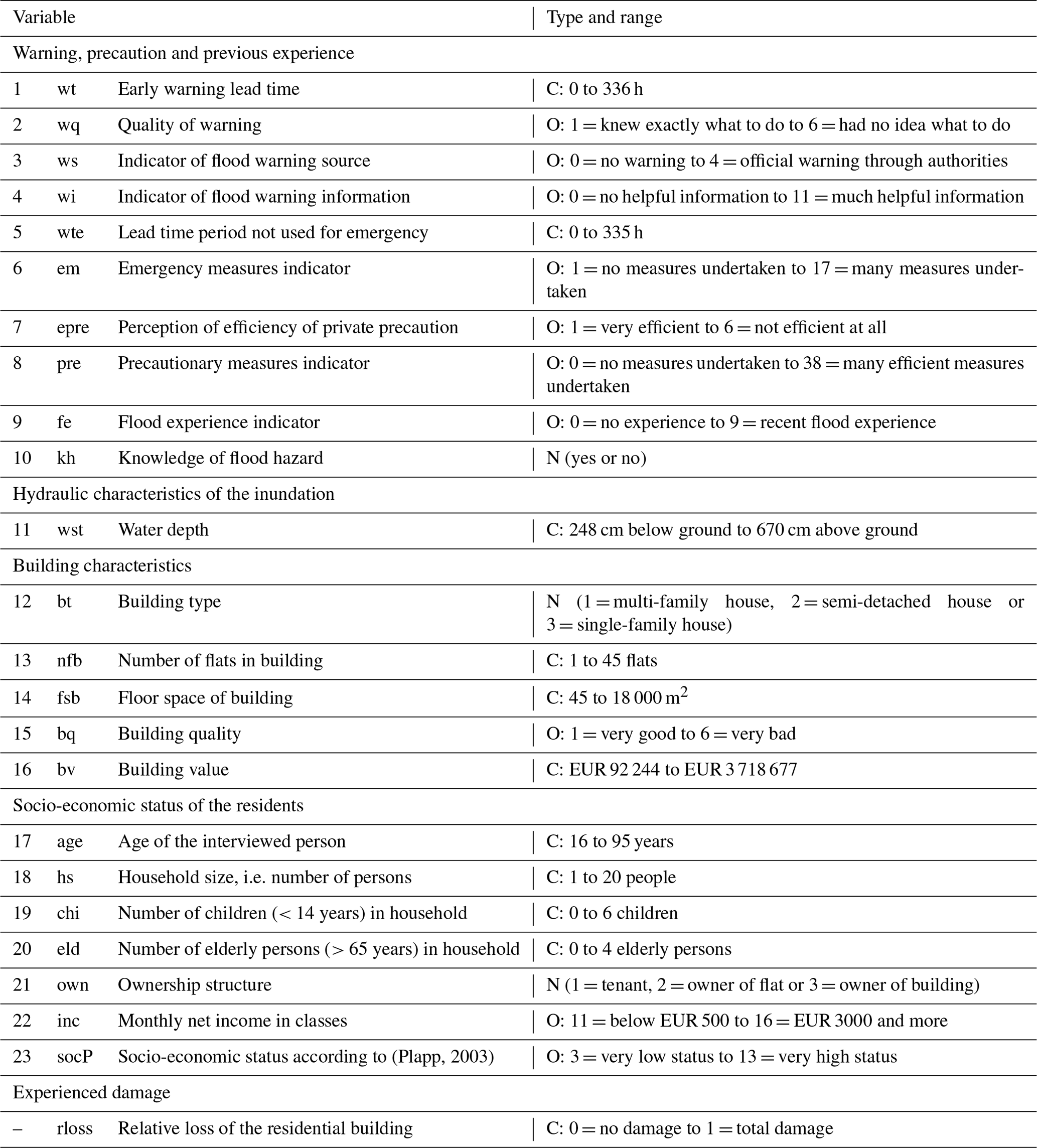
CATI surveys were conducted with affected private households ex post major floods in Germany. The regional focal points of flood impacts were the Elbe catchment in eastern Germany and the Danube catchment in southern Germany. Particularly noteworthy are the floods of 2002 and 2013, which caused economic losses of EUR 11.6 billion (reference year 2005) and EUR 8 billion respectively in Germany (Thieken et al., 2006, 2016). With EUR 1 billion in economic damage, the city of Dresden at the Elbe River in Saxony had been a hotspot of flood impacts during the August 2002 flood (Kreibich and Thieken, 2009). In August 2002, flash floods triggered by record-breaking precipitation and numerous levee failures caused widespread flooding along the Elbe River and its tributaries in Saxony and Saxony-Anhalt as well as along the Regen River and other southern tributaries to the Danube River in Bavaria (Schröter et al., 2015). The magnitude of flood peak discharges along these rivers well exceeded a statistical return period of 100 years (Ulbrich et al., 2003). In May 2013 a pronounced precipitation anomaly with subsequent extreme precipitation at the end of May and beginning of June caused severe flooding in June 2013, especially along the Elbe and Danube rivers, with new water level records and major dike breaches both at the Elbe and Danube rivers (Conradt et al., 2013; Merz et al., 2014; Schröter et al., 2015). The magnitude of flood peak discharges exceeded statistical return periods of 100 years along the Elbe, Mulde and Saale tributaries and along the Danube and Inn River in Bavaria (Blöschl et al., 2013; Schröter et al., 2015). With 180 questions, the CATI surveys cover a broad range of flood-impact-related factors including building characteristics, effects of warnings, precaution and the socio-economic background of households. The survey campaigns for different floods are consistent in terms of acquisition methodology, type and scope of questions. The interviewees were randomly selected from lists of potentially affected households along inundated streets which have been identified from satellite data, flood reports and press releases. With an average response rate of 15 %, in total 3056 interviews have been completed. For further details about the surveys and data processing, refer to Kienzler et al. (2015) and Thieken et al. (2005, 2017). Building on the findings of previous work (Merz et al., 2013; Schröter et al., 2014), for this study 23 variables have been preselected with a focus on building characteristics, flood intensity at the building and socio-economic status as well as warning, precaution and previous flood experience (Table 1). In addition, relative loss to the building has been determined as the ratio of reported actual losses and the building value (replacement cost) at the time of the flood event (Elmer et al., 2010). Hence, it describes the degree of building damage on a scale from 0 (no damage) to 1 (total damage). Building values are based on the standard actuarial valuation method of the insurance industry in Germany (Dietz, 1999), which estimates replacement costs using information about the floor space, basement area, number of storeys, roof type, etc. that are available from CATI data. Relative loss to the building and water depth (“wst”) at the building are the key variables from the CATI data set used in this study. The variable rloss is used to learn predictive models and to evaluate their performance. Consequently, the records in the CATI data set without values for rloss are removed. This reduces the number of available records from 3056 to 2203. The variable wst is the most commonly used predictor in flood vulnerability modelling (Gerl et al., 2016) because it is a highly relevant characteristic of flood intensity, and it is usually available from hydrodynamic numerical simulations; wst from CATI is a continuous variable with a length unit in centimetres. Negative values represent a water level below the ground surface, which affects only the basement of a building.
(Plapp, 2003)Table 1Preselected variables from CATI surveys; C: continuous, O: ordinal, N: nominal-scaled variables.
2.2 OpenStreetMap data
OSM is a free web-based map service built on the activity of registered users who contribute to the database by adding, editing or deleting features based on their local knowledge. The contributors use GPS devices and satellite as well as aerial imagery to verify the accuracy of the map. OSM is an open-data project, and the cartographic information can be downloaded, altered and redistributed under the Open Data Commons Open Database License (ODbL) (OpenStreetMap Contributors, 2020). Among the so-called volunteered geographic information (VGI) projects (Goodchild, 2007), OSM is the most widely known. OSM data provide information about building locations, footprint geometries, occupancy and other characteristics. The positional accuracy of OSM data, as well as the completeness of the database in respect to the number of mapped objects present in the real world, is nowadays considered satisfactory for most developed countries and urban areas (Barrington-Leigh and Millard-Ball, 2017; Hecht et al., 2013). On the contrary, information on object attributes such as road names or building types is often scarce and inconsistent. The tag “building” is used to identify the outline of a building object in OSM. The majority of buildings (82 %) have no further description, and only 12 % are specified as primarily “residential” or a single-family “house” (https://taginfo.openstreetmap.org/keys/building#values, last access: 28 February 2020). Therefore, the filtering for residential buildings from the OSM database uses the underlying “residential” land use information of OSM. By joining the land use information to the building polygons, those of residential occupation can be identified and selected.
2.3 Data preparation
The OSM and CATI data sets have been conflated in order to link the empirically observed variables rloss and wst with OSM data for individual residential buildings. This operation uses the geolocation information of both data sources. The CATI data are provided with address details including community, postal code, street name and the house number ranges in blocks of five numbers. Geocoding algorithms including open web API (application programming interface) services like Google (https://developers.google.com/maps/documentation/geolocation/overview, last access: 3 February 2021), Photon (https://photon.komoot.io/, last access: 3 February 2021) and Nominatim (https://nominatim.org/, last access: 3 February 2021) were applied to obtain geocoordinates for the address information from the interview data.
OSM is a spatial data set including georeferenced building outlines. The geolocated interviews are spatially matched with OSM building polygons using an overlay operation which merges interview points with OSM building polygons. In view of limited address details regarding the building house number ranges and inherent inaccuracies of geocoding databases and algorithms (Teske, 2014), a buffer radius of 5 m has been used to correct for offsets between geocoding points and building polygons. CATI records which still could not be matched with OSM geometries and with obviously erroneous geolocations, e.g. position is far away from flood-affected areas or urban settlements, have been removed from the data set. After these steps 1649 records remain from the original set of CATI surveys. The spatial distribution of these data points highly concentrates on the Elbe catchment (1234 records) including Dresden (310 records) and on the Danube catchment (105 records) (Fig. 1)
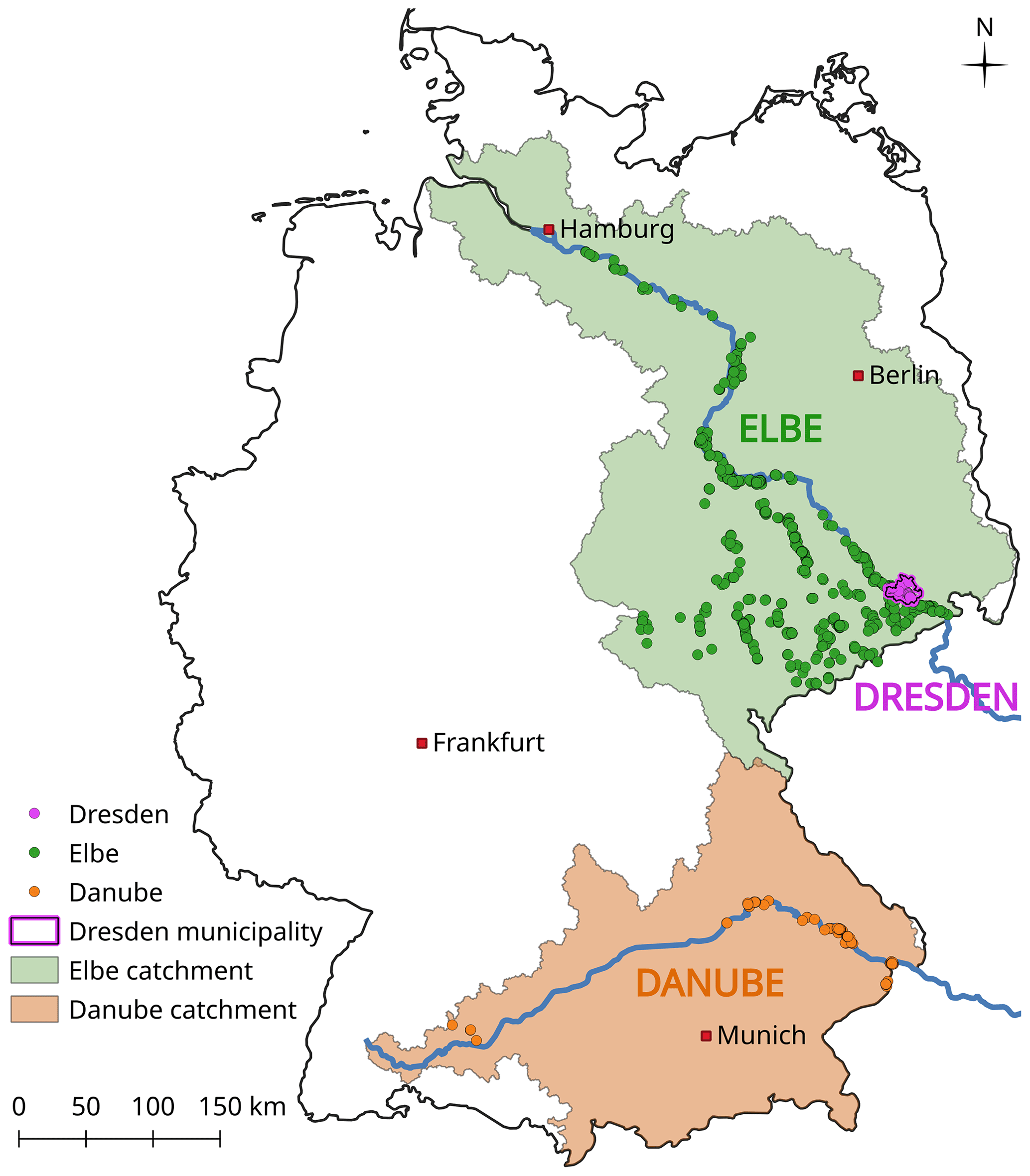
Figure 1Regional subdivision of the data set for spatial split-sample testing (Dresden municipality, the Elbe catchment and the Danube catchment).
2.4 Numerical measures
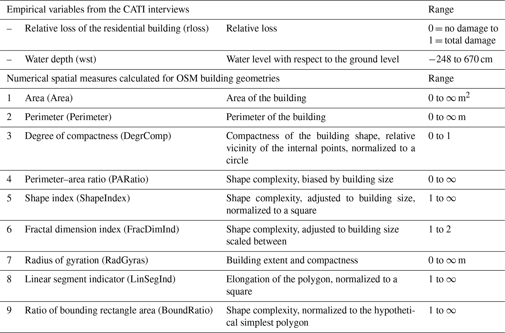
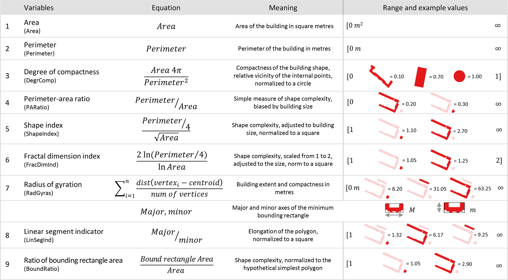
Information about the building geometry is useful to support the estimation of flood losses to residential buildings (Schröter et al., 2018). Building on this knowledge, numerical spatial measures are calculated for OSM building footprints with the aim to add potential explanatory variables to the estimation of relative loss to residential buildings. For this purpose, image analysis algorithms typically used in landscape ecology are adopted. These algorithms calculate numerical spatial measures like area, perimeter, elongation and complexity based on the analysis of geometries identified in aerial or remote sensing images (Jung, 2016; Lang and Tiede, 2003; Rusnack, 2017). The numerical spatial measures are calculated for each OSM building polygon and are compiled in Table 2 along with the other CATI variables that are used to derive flood vulnerability models. The meaning of these spatial measures, the equations, and range of values and examples are listed in the Appendix A1.
Table 2Variables of the amended OSM data set for each building object
We analyse the created data set with two main objectives. First, we strive to identify those variables from Table 2 which are most useful for explaining relative loss to residential buildings. Second, we aim to derive flood vulnerability models for residential buildings and to test these models for spatial transfers across regions. The data analysis workflow including data pre-processing, model learning, model selection and model transfer is illustrated in Fig. 2. The data pre-processing steps with data preparation and numerical spatial measures have been described in the previous section. For model learning and model transfer we use the random forest (RF) machine learning algorithm introduced by Breiman (2001).
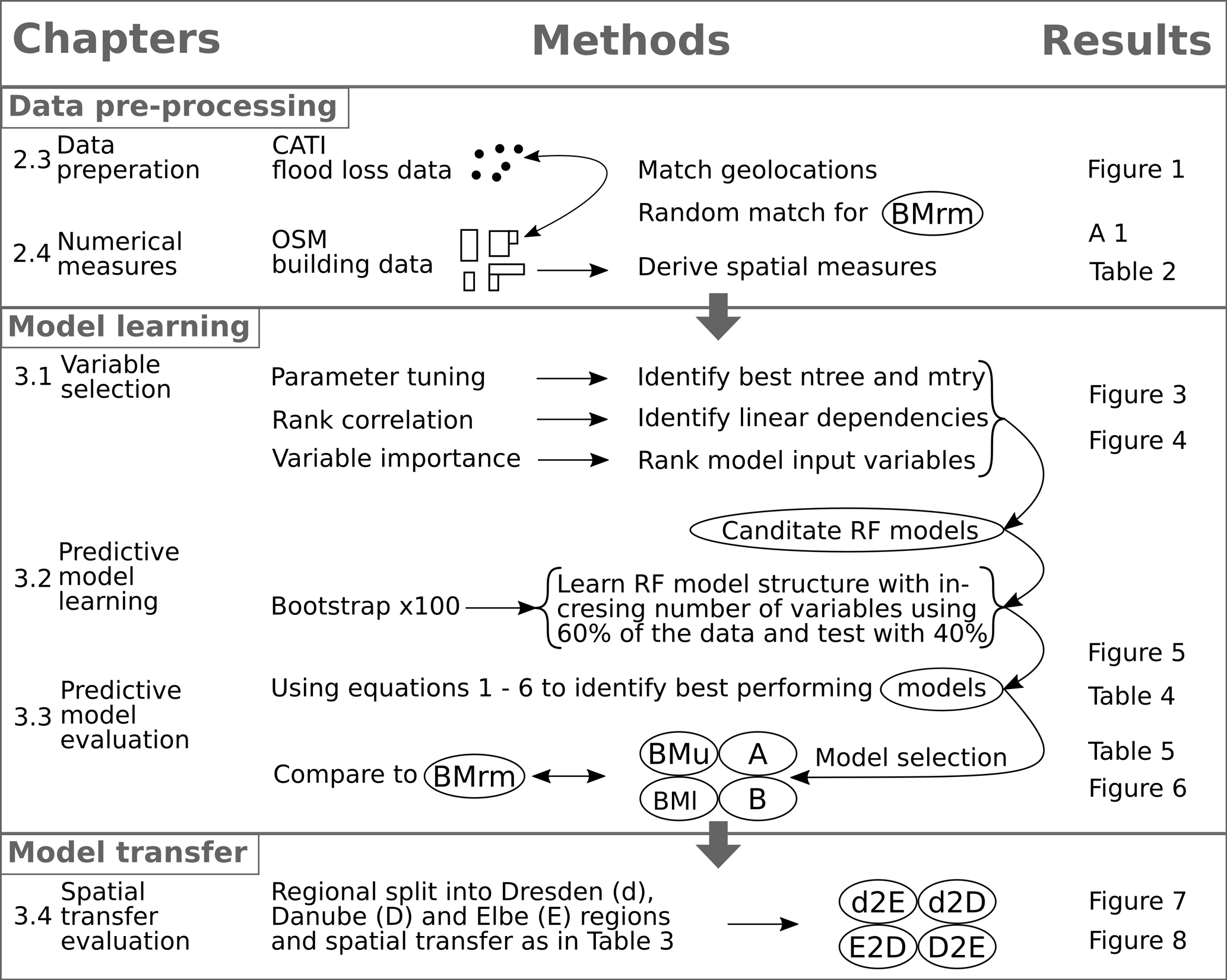
Figure 2Data pre-processing, model learning and model transfer workflow with BMu (upper-benchmark model); BMl (lower-benchmark model); BMrm (benchmark model with random match of interview locations with OSM building data); A (random forest model using eight predictors); B (random forest model using eight predictors); and model transfers d2E (learning with Dresden and predictions for Elbe), d2D (learning with Dresden and predictions for Danube), E2D (learning with Elbe and predictions for Danube) and D2E (learning with Danube and predictions for Elbe).
RFs are an extension of the classification and regression tree (CART) algorithm (Breiman et al., 1984), which aims to identify a regression structure among the variables in the data set. Regression trees recursively subdivide the space of predictor variables to approximate a non-linear regression structure. This subdivision is driven by optimizing the accuracy of local regression in these regions, which, by repeated partitioning, leads to a tree structure. Predictions are made by following the division criteria along the nodes and branches from the root node to the leaves, which finally contain the predicted value for a given set of input variables. RFs make predictions based on a large number of decision trees, i.e. a forest, which is learned by randomly selecting the variables considered for splitting the features space of the data. RFs incorporate bootstrap aggregation (bagging) as a simple and powerful ensemble method to reduce the variance of the CART algorithm. In comparison to single trees, RFs are more suitable to identify complex patterns and structures in the data (Basu et al., 2018). As an ensemble approach, RFs learn a regression tree for a number of bootstrap replica of the learning data. This results in a number of trees (“ntree”) forming a forest of regression trees. To reduce correlation between trees, the RF algorithm randomly selects a subset of variables (“mtry”) which are evaluated for dividing the space of predictor variables. This efficiently reduces overfitting and makes RF less sensitive to changes in the underlying data. Each bootstrap replica is created by randomly sampling with replacement about two-thirds of observations from the original data set. The remaining data are indicated as out-of-bag (OOB) observations and are used for evaluating the predictive accuracy of the tree, in terms of the OOB error. For regression trees the OOB error is the mean squared sum of residuals. For loss estimation, the predictions of all trees are combined by aggregating the individual predictions as the mean prediction from the forest. The predictions of the individual trees, i.e. from the ensemble of models, provide an estimate of predictive uncertainty.
For variable selection and predictive model learning RFs provide a concept to quantify the importance of candidate explanatory variables which allow for selecting the subset of most relevant variables. RFs are also an efficient algorithm to learn predictive models from heterogeneous data sets with complex interactions and with different scales like continuous or categorical information (Huang and Boutros, 2016).
RF predictive model performance is sensitive to specifications of the algorithm parameters mtry and ntree (Huang and Boutros, 2016). Therefore, the optimum values for both parameters are identified as those which yield minimum OOB errors on an independent data set. For parameter tuning, we pursue the variation approach implemented by Schröter et al. (2018) by selecting parameters from a broad and comprehensive range of values, ntree ∈ [100, 500, 1000, 2000, 3000, … 15 000] and mtry ∈ [, , 23] with p as the number of candidate predictors, and derive RF models for each combination. For each pair of chosen values, the algorithm is repeated 100 times to account for inherent data variability. The optimum parameters will minimize the prediction error on the OOB sample data. Using the optimum RF parameter settings, we derive predictive models for rloss.
3.1 Variable selection
The first step in model learning is the selection of variables to be used as predictors in the model. The analysis of the Spearman’s rank correlation between the variables gives a first insight into the linear dependency structure of the data set. Furthermore, RF supports the evaluation and ranking of potential predictors by quantification of variable importance which also accounts for variable interaction effects. The importance of a selected variable is evaluated by calculating the changes of the squared error of the predictions when the values of that variable are randomly permuted in the OOB sample. The increase of the average error will be larger for more important variables and smaller for less important variables. On this basis it is possible to decide which variables to include in a predictive model. The outcomes of variable importance evaluations are sensitive to the RF algorithm parameters mtry and ntree (Genuer et al., 2010). Therefore, to achieve stable results for these analyses, we implement a robust approach which averages the outcomes of multiple runs with variations in RF parameters (Schröter et al., 2018): ntree ∈ [500, 1000, 1500, 2000, … 5000], whereby each tree is repeatedly built for mtry ∈ [, , 2], with p as the number of candidate predictors, which correspond to the lower limit, the default value and the upper limit, suggested by (Breiman, 2001). Following this procedure, the potential explanatory variables of our data set (Table 2) are evaluated and ranked according to their relative importance to predict rloss.
3.2 Predictive model learning
Variable selection needs to be considered as an essential part of the model evaluation process. Therefore, candidate RF models using different numbers of variables are assessed in terms of predictive performance for independent data.
The OSM-based numerical spatial measures differentiate building form and shape complexity. To gain further insights into the suitability of these variables for flood vulnerability modelling, we incrementally add explanatory variables to the learning data set. Based on the outcomes of variable importance ranking the learning set is expanded variable by variable, and models of increasing complexity are learned (cf. Table 2). From the comparison of model predictive performance between these candidate models, the best balance between model performance and number of input variables is assessed. This is implemented by bootstrapping the splitting of the data into subsets for learning (60 %) and testing (40 %) with 100 iterations.
Further, for an independent assessment of OSM-based vulnerability model performance we consider two benchmark models. We argue that the set of CATI variables (Table 1) represents the most detailed data set available for flood loss estimation of residential buildings (Merz et al., 2013; Schröter et al., 2014; Thieken et al., 2016). Therefore, a RF model is learned using all 23 CATI predictors as an upper benchmark (BMu). In contrast, a RF model using only wst as a predictor is learned as a lower benchmark. The reasoning is that using extra variables in addition to wst will improve the predictive performance of the models (Schröter et al., 2016, 2018). As described in Sect. 2.3, the detail of geolocation information from CATI data is limited to ranges of house numbers. Therefore, we face uncertainty in whether CATI data and OSM building footprints have been matched correctly. To assess the potential implications of this source of uncertainty, we derive a model (BMrm) which is based on a data set with rloss and wst observations randomly assigned to OSM building footprints. We keep the RF modelling approach for the benchmark models consistent to ensure that any observed difference in model performance stems from differences in the underlying input variables.
3.3 Predictive model evaluation
Model predictive performance is evaluated by comparing predicted (P) and observed (O) rloss values from the validation sample using the following metrics. In these metrics RF predictions are evaluated for the median prediction (P50) derived from the ensemble of individual tree predictions.
Mean absolute error (MAE) quantifies the precision of model predictions, with smaller values indicating higher precision:
Mean bias error (MBE) is a measure of accuracy, i.e. systematic deviation from the observed value. Unbiased predictions yield a value of 0; underestimation results in negative; and overestimation in positive values:
Mean squared error (MSE) combines the variance of the model predictions and their bias. Again, smaller values indicate better model performance:
The ensemble of model predictions from the RF models offers insight into prediction uncertainty. This property is analysed by evaluating the 90 % quantile range, i.e. the difference between the 5 % quantile and 95 % quantile in relation to the median, as a measure of ensemble spread:
with the 95 % quantile, 5 % quantile and 50 % quantile, i.e. the median of the predictions. QR90 (quantile range) is a measure of sharpness with smaller values indicating a smaller prediction uncertainty.
Reliability of model predictions is quantified in terms of the hit rate (HR) (Gneiting and Raftery, 2007):
HR calculates the ratio of observations within the 95 %–5 % quantile range of model predictions. For a reliable prediction HR should correspond to the expected nominal coverage of 0.9.
HR and QR90 are combined to the interval score (IS), which accounts for the trade-off between HR values and QR90 ranges (Gneiting and Raftery, 2007):
3.4 Spatial-transfer evaluation
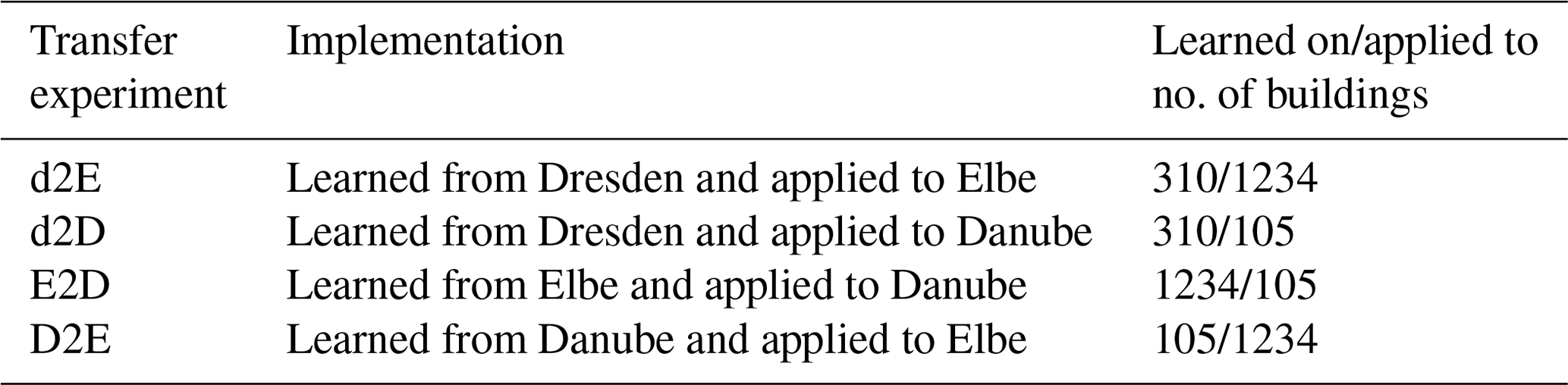
We investigate the question of whether the consistent data basis of OSM-derived numerical spatial measures supports the transfer of flood vulnerability models across regions by splitting the available data set into subsets for different regions affected by major floods. The CATI data are mainly located in the Elbe and Danube catchments in Germany, which are the regions mostly affected by inundations and flood impacts. This suggests a regional subdivision of the empirical data set according to these river basins for the investigation of spatial model transfer. In detail we partition the data set between the metropolitan area of Dresden (Saxony), the Elbe catchment (Saxony, Saxony-Anhalt and Thuringia) and the Danube catchment (Bavaria and Baden-Württemberg); see Fig. 1. This split is applied irrespective of the CATI survey campaign year, and thus the regional subsets contain records from different flood events. The idea is to investigate examples with a small set of learning data for a small specific region (Dresden), a large learning data set from an extended region (Elbe catchment) and a small set of learning data from an extended region (Danube catchment). The details for the learning and transfer applications are listed in Table 3. For these three regions we learn RF models using the selected variables and assess their predictive performance when transferred to the other regions. As we use a completely independent data set for model transfer testing, no additional bootstrap on top of RF internal bootstrapping is required.
Random forest OOB errors are sensitive to the choice of RF parameters mtry and ntree. From the variation of RF parameters we observe that OOB errors decrease with smaller values for mtry and larger numbers of trees in a forest (ntree); see Fig. 3.
The coloured bands represent the 90 % quantile range of OOB values from the 100 bootstrap repetitions for each RF algorithm configuration and illustrate the inherent variability of input variables in the learning data set. The colour code distinguishes the number of variables used to determine splits at each node (mtry). For mtry = 2 the smallest OOB errors are achieved throughout the variations in the number of trees (ntree). This value represents the lower bound of recommended values for mtry in RF regression models (Breiman, 2001). For smaller values of mtry less variables are considered for splitting the space of predictor variables, which reduces the correlation between individual trees of the forest. Further, increasing values of ntree asymptotically approximate smaller OOB values. It appears that for the given data set OOB values are virtually stable above ntree = 7000. As the computational effort increases with larger forests it has to be balanced with improvements regarding predictive performance. Building on these results we use RF parameters mtry = 2 and ntree = 7000, which are comparable to those used by Schröter et al. (2018).
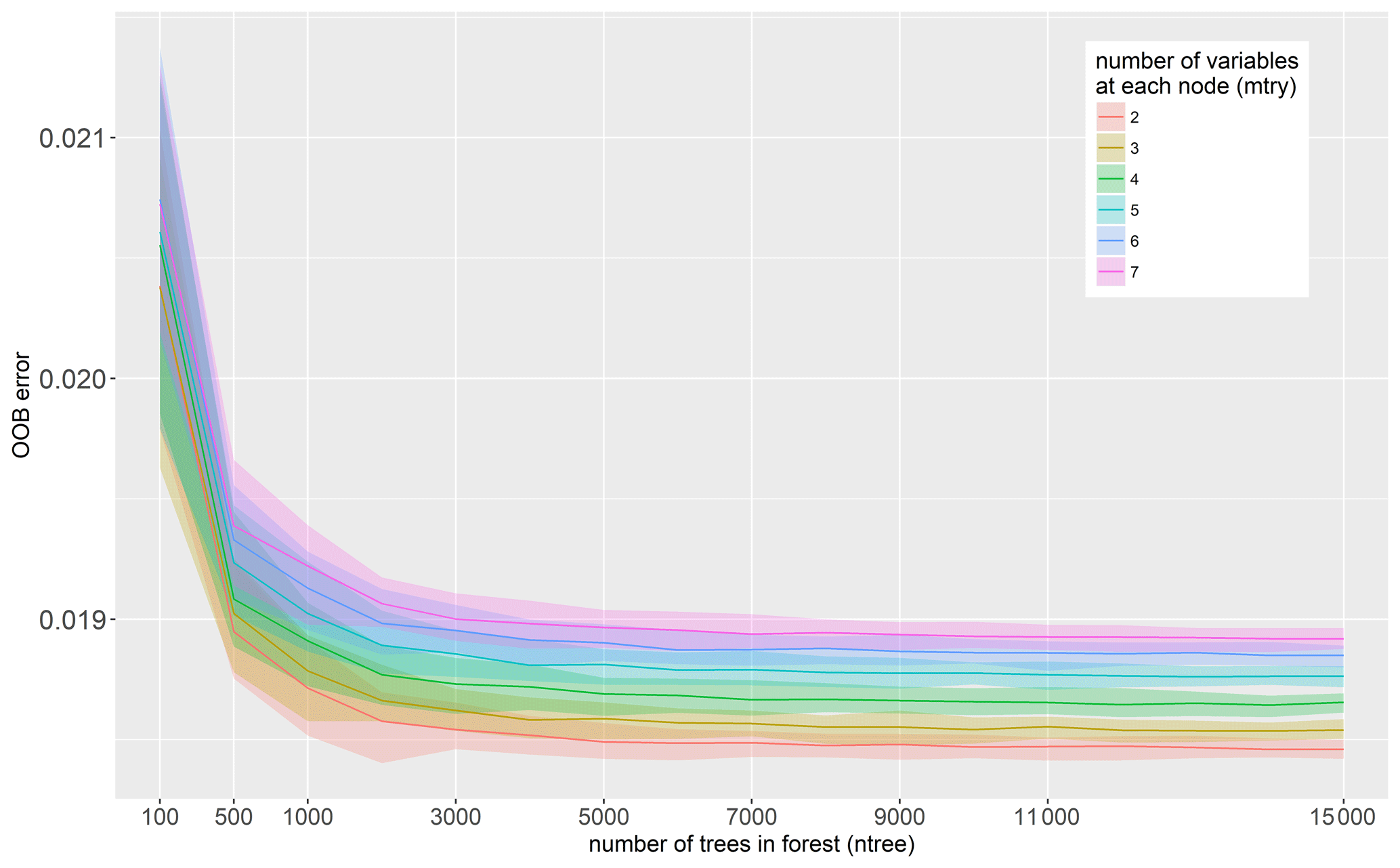
Figure 3Out-of-bag error for variations of mtry and ntree RF parameters. Colour bands represent the variation range of OOB errors obtained from 100 bootstrap repetitions.
4.1 Variable selection and predictive model learning
The numerical spatial measures (Table 2 and Appendix A1) evaluate properties of the building footprints including area, perimeter and elongation of main building axes. Accordingly some of these variables are strongly correlated (Fig. 4). The Spearman’s rank correlation matrix of the variables confirms a high degree of correlation in the data set, as for instance between Area, Perimeter and RadGyras. In contrast, the spatial measures are only slightly correlated with wst and rloss. The presence of multi-colinearity may influence the analysis of variable importance (Gregorutti et al., 2017). The robust importance analysis uses different RF parameter settings and reports an average importance rank, which alleviates this problem.
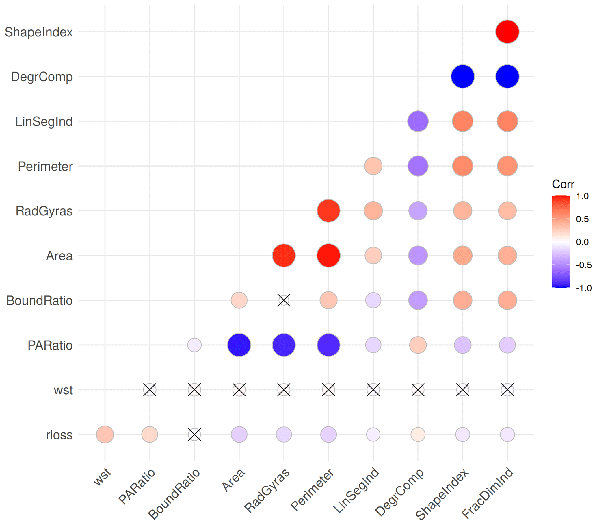
Figure 4Spearman’s correlation of model variables (significance level of 1 %); non-significant correlations are crossed out.
The variable wst ranks first in the importance analysis (results not shown), which confirms common knowledge in flood loss modelling (Gerl et al., 2016; Smith, 1994). In comparison to wst, the numerical spatial measures of OSM building footprints have clearly smaller importance values with relatively small differences between them. In terms of building characteristics, both spatial measures which express the size and extension of the building (e.g. Area and Perimeter) and spatial measures which describe building compactness and shape complexity (e.g. PARatio, RadGyras, LinSegInd and BoundRatio) seem to add information to better estimate relative building loss. The following order of importance was determined for the variables: wst, PARatio, RadGyras, Area, LinSegInd, BoundRatio, Perimeter, DegrComp, FracDimInd and ShapeIndex. Predictive performance tests for models with 2 to 10 variables (Fig. 5 and Table 4) build on this order of importance.
However, the outcome of the variable importance analysis does not suggest a clear selection of features to be included in a predictive flood vulnerability model. The model-predictive-performance-based assessment of variables uses an increasing number of variables following their ranking order of variable importance in the RF modelling. The predictive performance is quantified in terms of MAE, MBE and MSE (Eqs. 1, 2 and 3) for 100 bootstrap repetitions. While the MAE is decreasing when additional variables are used with an overall minimum for a model using six variables, including more than six variables tends to increase MAE again (Fig. 5). However, regarding MBE these changes go in an opposite direction. We observe the smallest MBE when only two variables are included. MBE then grows continuously for using up to seven variables and then slightly reduces when more variables are used. The increase in precision expressed by the smaller MAE is accompanied with a reduction of accuracy reflected by an increasing MBE. This yields an almost-balanced performance in terms of MSE for all models tested.

Figure 5Predictive performance of models using an increasing number of variables in order of their importance. Smaller MAE and MSE values and MBE values close to 0 indicate better performance; cf. Eqs. (1)–(3).
Looking into the sharpness of model predictions, the quantile range (QR90) is getting larger with an increasing number of model variables, which reflects larger uncertainty (Table 4). In terms of model reliability (HR), an increasing number of model variables achieves better performance statistics up to using eight variables. The combination of both QR and HR in the interval score (IS) shows a similar pattern.
Table 4Model performance metrics for models using an increasing number of variables arranged in the order of wst, PARatio, RadGyras, Area, LinSegInd, BoundRatio, Perimeter, DegrComp, FracDimInd and ShapeIndex. Best performance values and selected models are in bold.
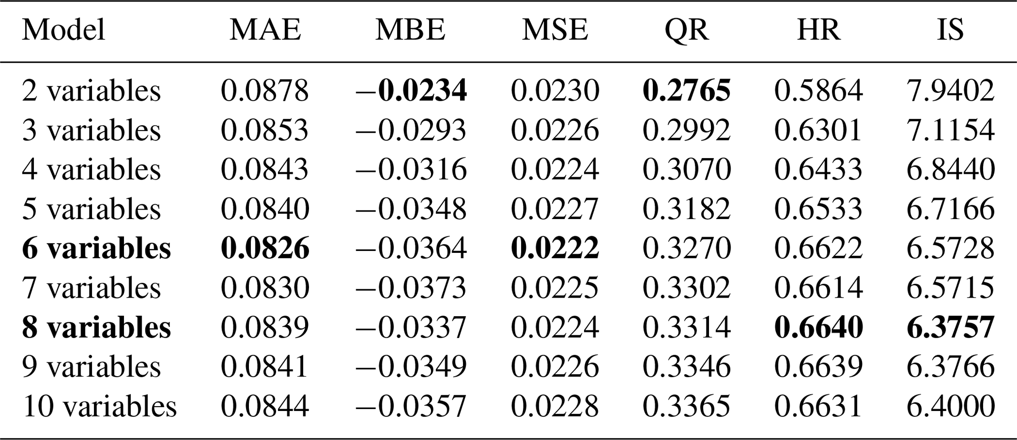
On the basis of these assessments two model alternatives are selected for further analysis: model A using eight variables, as it provides the most reliable model predictions, and model B using six variables, which provide the highest precision and balance between accuracy and precision. In detail model B uses the variables wst, PARatio, RadGyras, Area, LinSegInd and BoundRatio. Model A, in addition, uses Perimeter and DegrComp as predictors.
4.2 Model predictive performance: model benchmarking
The OSM models A and B are benchmarked with a model that uses all information available from the CATI surveys as an upper benchmark (BMu) and a model that uses only water depth as predictor as a lower benchmark (BMl). The performance statistics achieved by models A and B for the complete data set (all events and regions) are slightly inferior to BMu but clearly better than the outcomes of BMl (Fig. 6). Both models A and B give very similar performance statistics with slightly higher precision (smaller MAE) but larger bias (MBE) for model B. In contrast, model A provides more reliable predictions indicated by larger HR and smaller IS (Table 6). The randomized benchmark model (BMrm) achieves a better performance than BMl but is inferior to models A and B (Fig. 6, Table 5). Hence, we are confident that the remaining uncertainty associated with the mapping of geolocations to building geometries does not affect the outcomes of our analyses. Overall, we note that including numerical spatial measures based on OSM building footprints add useful information to predict loss to residential buildings. The numerical spatial measures included in the models are all directly calculated using building footprints. Therefore, a larger number of variables used for loss estimation does not imply increased efforts to collect data. From this perspective the cost of using model A or B is equal. The RF algorithm strives to reduce overfitting when large numbers of predictors are included, and thus the parsimonious modelling principle can be relaxed. A possible negative effect of overfitting when using more predictors should manifest in spatial-transfer applications.
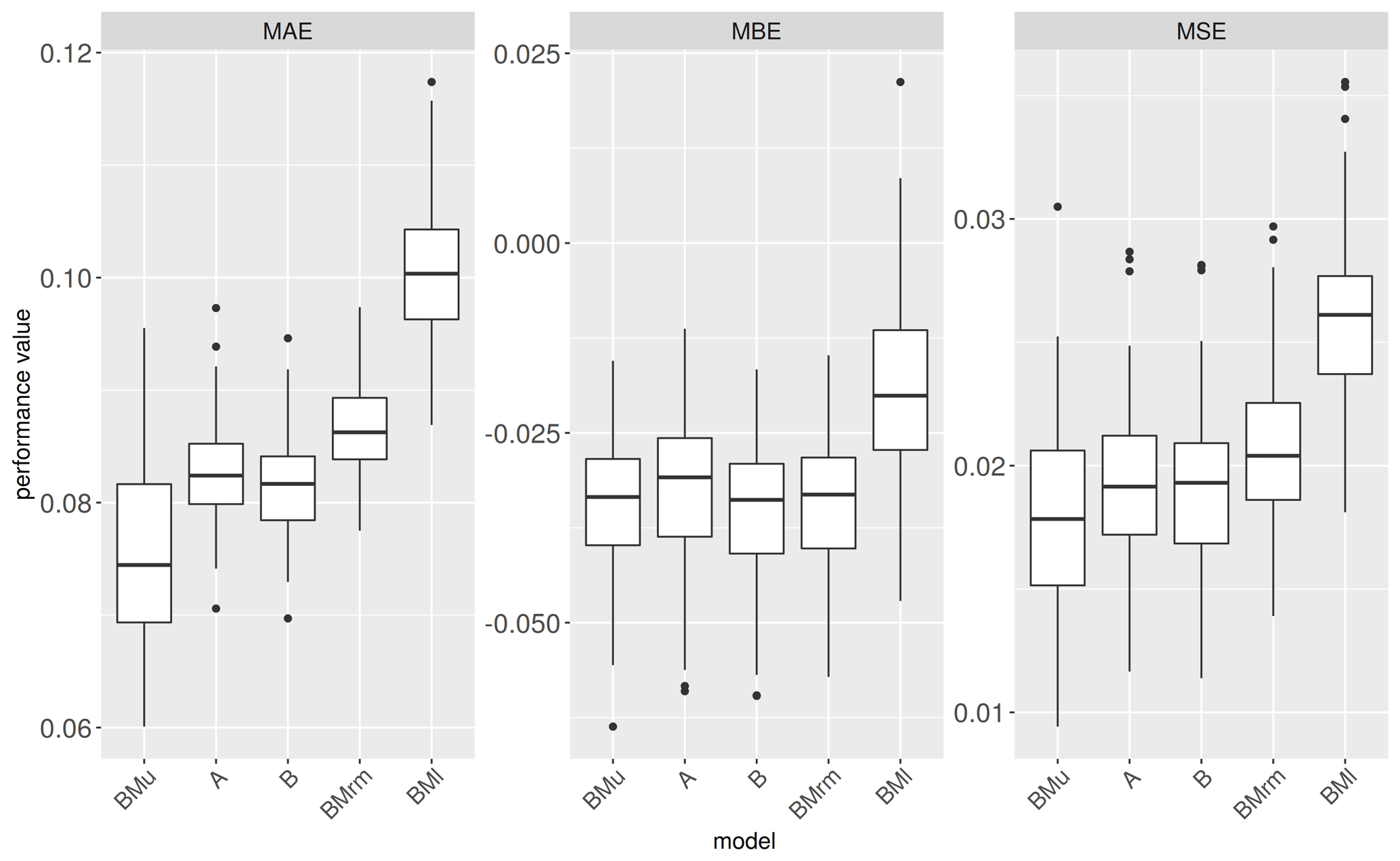
Table 5Model precision, accuracy and reliability performance metrics for OSM-based models and benchmark models.

4.3 Spatial-transfer testing
The predictive performance of RF models is tested in regional-transfer applications. For this purpose, the RF models A and B as well as the benchmark models BMu and BMl, as specified in the previous section, are learned using regional subsets of the data and applied to predict flood losses in a different region; see Sect. 3.4 and Table 3 for details about the regional subdivision of data and spatial-transfer experiments. Learning models with a regional subset of data and applying the models to other regions results in a drop of predictive performance in comparison to the case when the entire data set is used for model learning, except for the case of d2E (Fig. 7). In most of the learning or transfer cases, BMu scores best in terms of precision and reliability, represented by the performance metrics MAE, MSE, HR and IS. Using only wst as a predictor (BMl) produces less precise and less reliable predictions as indicated by larger MAE and MSE, as well as smaller HR and larger IS. While the performance of models A and B is very similar, model A, using eight predictors, more reliably predicts residential loss (larger HR and smaller IS), and model B, using six predictors, provides more accurate (MBE closer to 0) and more precise predictions (smaller MAE and MSE). Hence, overfitting does not seem to be an issue when more input variables are used. In contrast to the model benchmark comparison (Sect. 4.4) BMu and BMl do not entirely frame the RF model performance values. Instead, models A and B in some cases achieve better and in other cases worse performance statistics. Generally speaking, the predictive performance differs more strongly between the regional-transfer settings than between the models (Fig. 7). This is more pronounced for precision and accuracy metrics (MAE, MBE and MSE) than for sharpness and reliability indicators (QR, HR and IS). Learning from the Dresden subset and transferring the model to the Elbe region (d2E) works best as is shown by the smallest MAE and MSE as well as an MBE closest to 0. Learning the models with the Danube subset and transferring them to the Elbe region (D2E) yields comparably small MAE and MSE values, but this is also the only case with a tendency to overestimate rloss resulting in a positive MBE. The models are struggling most to predict loss when they are learned with the Dresden subset and transferred to the Danube region (d2D), showing the lowest precision and accuracy. In turn, extending the learning subset to the Elbe region improves the transfer to the Danube (E2D). Concerning predictive uncertainty and reliability, learning with the Danube subset yields large QRs, which however only partly cover the observed loss values reflected in comparably low HR and high IS (D2E). Learning from Dresden or Elbe and transferring to Elbe or Danube (d2E, d2D and E2D) produces sharper predictions, but still the models differ in reliability, i.e. covering the observed values within their predictive uncertainty ranges (HR). In this respect, the upper benchmark model (BMu) performs best. The differences between models A and B are small, and both are better than the lower benchmark model (BMl) and almost similar to BMu for the transfer cases between the regions Elbe and Danube (E2D and D2E).
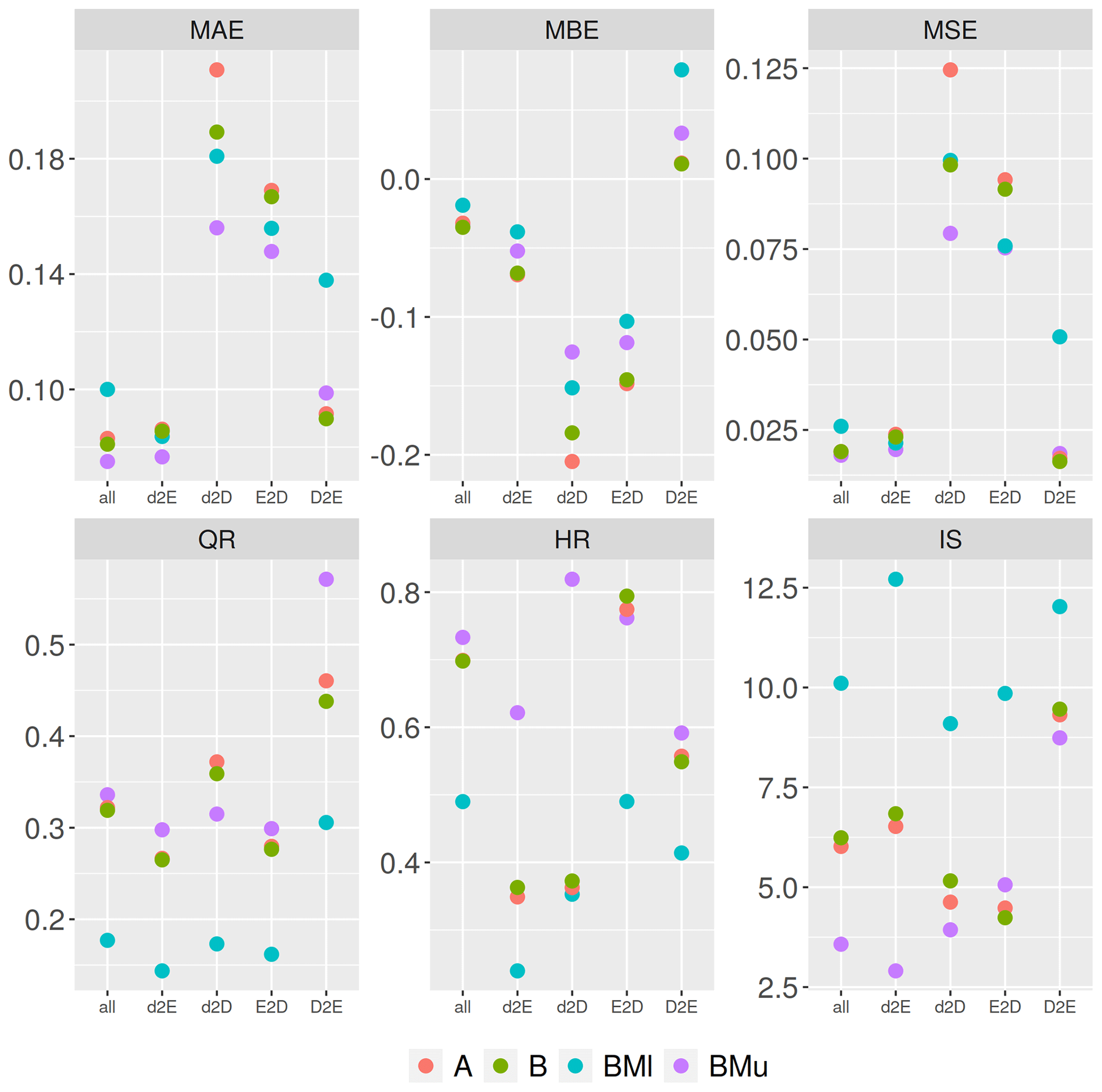
Figure 7Model performance metrics in regional transfer. Models A and B based on spatial numerical measures calculated for OSM building footprints; benchmark models BMl and BMu based on CATI survey data. Transfer experiments d2E, d2D, E2D and D2E as described in Table 3; “all” refers to using all records from all regions; cf. Table 5.
With 105 records the Danube data set is the smallest sub-sample. It has a smaller variability and range of values for most numerical spatial measures in comparison to the Dresden and Elbe regional sets (Fig. 8).

Figure 8Scatterplots of numerical spatial measures and relative loss in regional sub-samples (Danube, Dresden and Elbe).
The geometric properties of the flood-affected residential buildings in the Danube region seem to differ from the affected residential buildings in the Elbe region. In the Danube subset, the area and perimeter of buildings tend to be smaller than in the Elbe region. Also, the values for spatial measures representing building shape complexity, for instance RadGyras, DegrComp and BoundRatio, indicate more compact building footprints in the Danube region than in the Elbe region. These differences can be attributed to different socio-economic characteristics as well as building practices in former East and West Germany and regional differences in building types (Thieken et al., 2007). With only 310 records, the Dresden sub-sample covers comparable ranges of observed variables as the Elbe subset (1234 records). Both subsets show largely similar relations between individual variables and rloss. Still, the Danube subset includes relatively many records with high rloss values, which are distributed along the whole spectrum of above-ground-level water depths (Fig. 8). In comparison, the Dresden subset comprises very few cases with high relative loss which is partly related to differing inundation processes. In the Elbe and Danube catchments large areas have been flooded as a consequence of levee failures. Hence, the relationship of model variables to high rloss values cannot be learned from this subset and thus is not represented well by the model. Therefore, this difference in the learning data may explain the positive bias introduced by learning the model in the Danube and transferring it to the Elbe and, vice versa, the pronounced negative bias introduced by learning the model in Dresden and transferring it to the Danube region. Viewed from a model performance perspective, the transfer applications show that a good agreement between learning and transfer data sets (e.g. d2E) produces more precise and reliable predictions than the transfer to regions with pronounced differences (e.g. d2D and D2E). Still from the Danube region with limited ranges of variable values, it is possible to obtain relatively precise and accurate predictions of relative building loss. This suggests that a broad variability of observed rloss values in the learning data set is an important control for the predictive capability of the model in other regions. In contrast, small samples with limited variability and only few records with high rloss values struggle with predicting rloss in other regions. This confirms insights that a model based on more heterogeneous data performs better when transferred in space (Wagenaar et al., 2018). Our findings also reveal that using numerical spatial measures derived from OSM building geometries does not resolve all problems of model transfer. As not many variables of building characteristics are available from OSM data, the spatial measures calculated from building footprints serve as proxy variables for these unavailable details. These proxies achieve comparable predictive performance as specific property level data sets as for instance collected via computer-aided telephone interview surveys represented by the BMu model. This model uses a broad range of variables to characterize vulnerability of residential buildings including details of building characteristics; socio-economic status of the household; and flood warning, precaution and previous flood experience (cf. Table 1). Still, this more comprehensive information does not result in a clearly better model predictive performance in transfer applications. Additional improvements can be expected from including local expert knowledge about inundation duration, flood experience and return period of the event into the modelling process (Sairam et al., 2019). Flood-event-related variables including flood type appear to be important information for estimating the degree of building loss because they describe differences in the damaging processes (Vogel et al., 2018). Other data sources have been used to enrich empirical data sets for learning flood loss models. This includes for instance information about the building age and floor area for living from Cadastre data (Wagenaar et al., 2017), number of storeys, building type, building structure, finishing level and conservation status from census data (Amadio et al., 2019). However, using these data did not result in a clear improvement in spatial model transfer. Using variables derived from OSM data increases the flexibility of the models to be applied in other regions because the accessibility and availability of OSM data reduces the effort of data collection, simplifies the preparation of input variables and ensures consistency of input data. The latter point is an important advantage because achieving consistency of input data has been stressed to cause large efforts in model transfers (Jongman et al., 2012; Molinari et al., 2020). The suggested RF models are based on an ensemble approach and thus provide a view to the predictive uncertainty of the model outputs. We have shown this to be a valuable detail in assessing the reliability of model predictions in spatial transfers. In cases where model performance cannot be tested with local empirical evidence, using model ensembles has been shown to provide more skilful loss estimates (Figueiredo et al., 2018).
The transfer of flood vulnerability models to regions other than those for which they have been developed often comes with reduced predictive performance. In this study we investigated the suitability of numerical spatial measures calculated for residential-building footprints, which are accessible from OpenStreetMap, to predict flood damage. Further we tested potential benefits from using this widely available and consistent input data source for the transfer of vulnerability models across regions. We develop a new data set based on OpenStreetMap data, which comprises variables representing building footprint dimensions and shape complexity, and we devise novel flood vulnerability models for residential buildings.
The geometric characteristics of building footprints serve as proxy variables for building resistance to flood impacts and prove useful for flood loss estimation. These model input variables are easily extracted by an automated process applicable to every type of building polygon. Hence, the models can be applied to areas where information about the footprint geometry of residential buildings is available. Also other data sources, e.g. cadastral data or data derived from remote sensing, can be used besides the OpenStreetMap data source. While the variables derived from building footprints ensure consistency and support transferability of models, the models remain context specific and should only be transferred to regions with comparable building geometric features as the learning data set.
The vulnerability models have been validated using empirical data of relative loss to residential buildings. Further, a benchmark comparison of the models has been conducted in spatial-transfer applications. The models give comparable performance to alternative multi-variable models, which use comprehensive and detailed information about preparedness, socio-economic status and other aspects of building vulnerability. In comparison to a model which uses only water depth as a predictor, they reduce model prediction errors (MAE by 20 % and MSE by 25 %) and increase the reliability of model predictions by a factor of 1.4.
OpenStreetMap is a highly popular and evolving data source with constantly increasing completeness and up-to-date data. In the future, the attributes of residential buildings are expected to provide additional details which are of interest for the characterization of building resistance to flooding. This includes for instance information about the building type, roof type, number of floors and building material and opens up further possibilities to refine the variables used for vulnerability modelling. These data could be further amended with other open-data sources including socio-economic statistical data. In view of a large variability of flood loss on the individual-building level, vulnerability modelling for individual buildings remains challenging and is subject to large uncertainty. Advances to the understanding of damage processes and the improvement of flood vulnerability modelling hence require an improved and extended monitoring of flood losses.
Flood damage data of the 2005, 2006, 2010, 2011 and 2013 events along with instructions on how to access the data are available via the German flood damage database, HOWAS21 (https://doi.org/10.1594/GFZ.SDDB.HOWAS21, GFZ German Research Centre for Geosciences, 2020). Flood damage data from the 2002 event were partly funded by the Deutsche Rückversicherung Aktiengesellschaft reinsurance company and may be obtained upon request.
OSM is an open-data project, and the cartographic information can be downloaded, altered and redistributed under the Open Data Commons Open Database License (ODbL) (OpenStreetMap Contributors, 2020).
In the presented study, the geographic data were processed in PostgreSQL 12.2 with the PostGIS 3.0.1 extension and R version 3.6.3 (29 February 2020) (R Core Team, 2020). The spatial measures were calculated in PostgreSQL and imported into R for further processing. The random forest model was built and applied in R with the use of the following packages: “randomForest 4.6-14” (Liaw and Wiener, 2002), “sf 0.6-3” (Pebesma, 2018, https://doi.org/10.32614/RJ-2018-009), “reshape2_1.4.3” (Wickham, 2007), “gdalUtilities_1.1.0” (O'Brien, 2020), “rpostgis_1.4.3” (Bucklin and Basille, 2018), “rgdal_1.4-8” (Bivand et al., 2019), “raster_3.0-7” (Hijmans, 2019), “RPostgreSQL_0.6-2” (Conway et al., 2017) and “tidyverse_1.3.0” (Wickham et al., 2019, https://doi.org/10.21105/joss.01686).
MC and KS conceived and designed the study. MC prepared and analysed the data with support from MS and KS. MC and KS wrote the first draft of the paper. HK helped guide the research through technical discussions. All authors reviewed the draft of the paper and contributed to the final version.
Authors Heidi Kreibich and Kai Schröter are members of the editorial board of Natural Hazards and Earth System Sciences.
This article is part of the special issue “Groundbreaking technologies, big data, and innovation for disaster risk modelling and reduction”. It is not associated with a conference.
The authors gratefully acknowledge the support by the German Research Network Natural Disasters (German Ministry of Education and Research (BMBF), no. 01SFR9969/5); the MEDIS project (BMBF; no. 0330688); the project “Hochwasser 2013” (BMBF; no. 13N13017); and a joint venture between the GFZ German Research Centre for Geosciences, the University of Potsdam and the Deutsche Rückversicherung Aktiengesellschaft (Düsseldorf) for the collection of empirical damage data using computer-aided telephone interviews. The authors further would like to thank Stefan Lüdtke and Danijel Schorlemmer (both from GFZ) for technical support with OSM data.
This research has been supported by Horizon 2020 (H2020_Insurance, grant no. 730381) and the EIT Climate-KIC (grant no. TC2018B_4.7.3-SAFERPL_P430-1A KAVA2 4.7.3).
The article processing charges for this open-access
publication were covered by a Research
Centre of the Helmholtz Association.
This paper was edited by Carmine Galasso and reviewed by four anonymous referees.
Alfieri, L., Feyen, L., Salamon, P., Thielen, J., Bianchi, A., Dottori, F., and Burek, P.: Modelling the socio-economic impact of river floods in Europe, Nat. Hazards Earth Syst. Sci., 16, 1401–1411, https://doi.org/10.5194/nhess-16-1401-2016, 2016. a
Amadio, M., Scorzini, A. R., Carisi, F., Essenfelder, A. H., Domeneghetti, A., Mysiak, J., and Castellarin, A.: Testing empirical and synthetic flood damage models: the case of Italy, Nat. Hazards Earth Syst. Sci., 19, 661–678, https://doi.org/10.5194/nhess-19-661-2019, 2019. a
Amirebrahimi, S., Rajabifard, A., Mendis, P., and Ngo, T.: A framework for a microscale flood damage assessment and visualization for a building using BIM–GIS integration, Int. J. Digit. Earth, 9, 363–386, https://doi.org/10.1080/17538947.2015.1034201, 2016. a
Apel, H., Aronica, G. T., Kreibich, H., and Thieken, A.: Flood risk analyses–how detailed do we need to be?, Nat. Hazards, 49, 79–98, https://doi.org/10.1007/s11069-008-9277-8, 2009. a, b
Barrington-Leigh, C. and Millard-Ball, A.: The world’s user-generated road map is more than 80 % complete, Plos One, 12, 1–20, https://doi.org/10.1371/journal.pone.0180698, 2017. a, b
Basu, S., Kumbier, K., Brown, J. B., and Yu, B.: Iterative random forests to discover predictive and stable high-order interactions, P. Natl. Acad. Sci. USA, 115, 1943–1948, https://doi.org/10.1073/pnas.1711236115, 2018. a
Bivand, R., Keitt, T., and Rowlingson, B.: rgdal: Bindings for the “Geospatial” Data Abstraction Library, available at: https://CRAN.R-project.org/package=rgdal (last access 4 March 2020), r package version 1.4–8, 2019. a
Blanco-Vogt, A. and Schanze, J.: Assessment of the physical flood susceptibility of buildings on a large scale – conceptual and methodological frameworks, Nat. Hazards Earth Syst. Sci., 14, 2105–2117, https://doi.org/10.5194/nhess-14-2105-2014, 2014. a
Blöschl, G., Nester, T., Komma, J., Parajka, J., and Perdigão, R. A. P.: The June 2013 flood in the Upper Danube Basin, and comparisons with the 2002, 1954 and 1899 floods, Hydrol. Earth Syst. Sci., 17, 5197–5212, https://doi.org/10.5194/hess-17-5197-2013, 2013. a
Breiman, L.: Random Forests, Mach. Learn., 45, 5–32, https://doi.org/10.1023/A:1010933404324, 2001. a, b, c, d
Breiman, L., Friedman, J., Stone, C. J., and Olshen, R. A.: Classification and Regression Trees, Taylor & Francis Ltd, Boca Raton, FL, USA, 1984. a
Bucklin, D. and Basille, M.: rpostgis: linking R with a PostGIS spatial database, The R Journal, 10, 251–268, available at: https://journal.r-project.org/archive/2018/RJ-2018-025/index.html (last access: 4 March 2020), 2018. a
Bui, Q.-T., Nguyen, Q.-H., Nguyen, X. L., Pham, V. D., Nguyen, H. D., and Pham, V.-M.: Verification of novel integrations of swarm intelligence algorithms into deep learning neural network for flood susceptibility mapping, J. Hydrol., 581, 124379, https://doi.org/10.1016/j.jhydrol.2019.124379, 2020. a
Cammerer, H., Thieken, A. H., and Lammel, J.: Adaptability and transferability of flood loss functions in residential areas, Nat. Hazards Earth Syst. Sci., 13, 3063–3081, https://doi.org/10.5194/nhess-13-3063-2013, 2013. a, b
Carisi, F., Schröter, K., Domeneghetti, A., Kreibich, H., and Castellarin, A.: Development and assessment of uni- and multivariable flood loss models for Emilia-Romagna (Italy), Nat. Hazards Earth Syst. Sci., 18, 2057–2079, https://doi.org/10.5194/nhess-18-2057-2018, 2018. a, b
Changnon, S. A.: Shifting economic impacts from weather extremes in the United States: A result of societal changes, not global warming, Nat. Hazards, 29, 273–290, 2003. a
Chinh, D. T., Gain, A., Dung, N., Haase, D., and Kreibich, H.: Multi-Variate Analyses of Flood Loss in Can Tho City, Mekong Delta, Water-Sui., 8, 6,https://doi.org/10.3390/w8010006, 2015. a
Conradt, T., Roers, M., Schröter, K., Elmer, F., Hoffmann, P., Koch, H., Hattermann, F., and Wechsung, F.: Comparison of the extreme floods of 2002 and 2013 in the German part of the Elbe River basin and their runoff simulation by SWIM-live, Hydrol. Wasserbewirts., 57, 241–245, https://doi.org/10.5675/HyWa_2013,5_4, 2013. a
Conway, J., Eddelbuettel, D., Nishiyama, T., Prayaga, S. K., and Tiffin, N.: RPostgreSQL: R Interface to the “PostgreSQL” Database System, available at: https://cran.r-project.org/web/packages/RPostgreSQL/index.html (last access: 4 March 2020), r package version 0.6-2, 2017. a
de Moel, H., Jongman, B., Kreibich, H., Merz, B., Penning-Rowsell, E. and Ward, P. J.: Flood risk assessments at different spatial scales, Mitig Adapt Strateg Glob Change, 20, 865–890, https://doi.org/10.1007/s11027-015-9654-z, 2015. a, b
Dietz, H.: Wohngebäudeversicherung Kommentar, VVW Verlag Versicherungswirtschaft GmbH, Karlsruhe, 2 Edn., 1999. a
Dottori, F., Figueiredo, R., Martina, M. L. V., Molinari, D., and Scorzini, A. R.: INSYDE: a synthetic, probabilistic flood damage model based on explicit cost analysis, Nat. Hazards Earth Syst. Sci., 16, 2577–2591, https://doi.org/10.5194/nhess-16-2577-2016, 2016. a, b
Elmer, F., Thieken, A. H., Pech, I., and Kreibich, H.: Influence of flood frequency on residential building losses, Nat. Hazards Earth Syst. Sci., 10, 2145–2159, https://doi.org/10.5194/nhess-10-2145-2010, 2010. a
Felder, G., Gómez-Navarro, J., Zischg, A., Raible, C., Röthlisberger, V., Bozhinova, D., Martius, O., and Weingartner, R.: From global circulation to local flood loss: Coupling models across the scales, Sci. Total Environ., 635, 1225–1239, https://doi.org/10.1016/j.scitotenv.2018.04.170, 2018. a
Figueiredo, R. and Martina, M.: Using open building data in the development of exposure data sets for catastrophe risk modelling, Nat. Hazards Earth Syst. Sci., 16, 417–429, https://doi.org/10.5194/nhess-16-417-2016, 2016. a
Figueiredo, R., Schröter, K., Weiss-Motz, A., Martina, M. L. V., and Kreibich, H.: Multi-model ensembles for assessment of flood losses and associated uncertainty, Nat. Hazards Earth Syst. Sci., 18, 1297–1314, https://doi.org/10.5194/nhess-18-1297-2018, 2018. a, b
Genuer, R., Poggi, J. ., and Tuleau-Malot, C.: Variable selection using random forests, Pattern Recogn. Lett., 31, 2225–2236, 2010. a
GFZ German Research Centre for Geosciences: HOWAS 21, Helmholtz Centre Potsdam, https://doi.org/10.1594/GFZ.SDDB.HOWAS21, 2020. a
Gerl, T., Kreibich, H., Franco, G., Marechal, D., and Schröter, K.: A Review of Flood Loss Models as Basis for Harmonization and Benchmarking, Plos One, 11, e0159791, https://doi.org/10.1371/journal.pone.0159791, 2016. a, b, c
Gneiting, T. and Raftery, A.: Strictly Proper Scoring Rules, Prediction, and Estimation, J. Am. Stat. Assoc., 102, 359–378, https://doi.org/10.1198/016214506000001437, 2007. a, b
Goodchild, M. F.: Citizens as sensors: the world of volunteered geography, Geojournal, 69, 211–221, https://doi.org/10.1007/s10708-007-9111-y, 2007. a
Gregorutti, B., Michel, B., and Saint-Pierre, P.: Correlation and variable importance in random forests, Stat. Comput., 27, 659–678, https://doi.org/10.1007/s11222-016-9646-1, 2017. a
Hasanzadeh Nafari, R., Ngo, T., and Lehman, W.: Calibration and validation of FLFArs – a new flood loss function for Australian residential structures, Nat. Hazards Earth Syst. Sci., 16, 15–27, https://doi.org/10.5194/nhess-16-15-2016, 2016. a
Hecht, R., Kunze, C., and Hahmann, S.: Measuring Completeness of Building Footprints in OpenStreetMap over Space and Time, ISPRS Int. J. Geogr. Inf., 2, 1066–1091, https://doi.org/10.3390/ijgi2041066, 2013. a, b
Hijmans, R. J.: raster: Geographic Data Analysis and Modeling, available at: https://CRAN.R-project.org/package=raster (last access: 4 March 2020), r package version 3.0-7, 2019. a
Hoeppe, P.: Trends in weather related disasters – Consequences for insurers and society, Weather Climate Extremes, 11, 70–79, https://doi.org/10.1016/j.wace.2015.10.002, 2016. a
Huang, B. and Boutros, P.: The parameter sensitivity of random forests, BMC Bioinformatics, 17, 331, https://doi.org/10.1186/s12859-016-1228-x, 2016. a, b
Irwin, A.: No PhDs needed: how citizen science is transforming research, Nature, 562, 480, https://doi.org/10.1038/d41586-018-07106-5, 2018. a
Jongman, B.: Effective adaptation to rising flood risk, Nat. Commun., 9, 1986, https://doi.org/10.1038/s41467-018-04396-1, 2018. a
Jongman, B., Kreibich, H., Apel, H., Barredo, J. I., Bates, P. D., Feyen, L., Gericke, A., Neal, J., Aerts, J. C. J. H., and Ward, P. J.: Comparative flood damage model assessment: towards a European approach, Nat. Hazards Earth Syst. Sci., 12, 3733–3752, https://doi.org/10.5194/nhess-12-3733-2012, 2012. a, b
Jung, M.: LecoS — A python plugin for automated landscape ecology analysis, Ecol. Inf., 31, 18–21, https://doi.org/10.1016/j.ecoinf.2015.11.006, 2016. a
Kienzler, S., Pech, I., Kreibich, H., Müller, M., and Thieken, A. H.: After the extreme flood in 2002: changes in preparedness, response and recovery of flood-affected residents in Germany between 2005 and 2011, Nat. Hazards Earth Syst. Sci., 15, 505–526, https://doi.org/10.5194/nhess-15-505-2015, 2015. a
Kreibich, H. and Thieken, A.: Coping with floods in the city of Dresden, Germany, Nat. Haz., 51, 423–436, https://doi.org/10.1007/s11069-007-9200-8, 2009. a
Kron, W.: Flood Risk = Hazard ⋅ Values ⋅ Vulnerability, Water Int., 30, 58–68, https://doi.org/10.1080/02508060508691837, 2005. a
Lang, S. and Tiede, D.: vLATE Extension für ArcGIS – vektorbasiertes Tool zur quantitativen Landschaftsstrukturanalyse, ESRI European User Conference 2003 Innsbruck, CDROM, (1986), 1–10, 2003. a
Liaw, A. and Wiener, M.: Classification and Regression by randomForest, R News, 2, 18–22, https://cran.r-project.org/doc/Rnews/Rnews_2002-3.pdf (last access: 3 February 2021), 2002. a
Lugeri, N., Kundzewicz, Z., Genovese, E., Hochrainer, S., and Radziejewski, M.: River flood risk and adaptation in Europe – assessment of the present status, Mitigation and Adaptation Strategies for Global Change, 15, 621–639, https://doi.org/10.1007/s11027-009-9211-8, 2010. a
Lüdtke, S., Schröter, K., Steinhausen, M., Weise, L., Figueiredo, R., and Kreibich, H.: A Consistent Approach for Probabilistic Residential Flood Loss Modeling in Europe, Water Resour. Res., 55, 10616–10635, https://doi.org/10.1029/2019WR026213, 2019. a, b
Merz, B., Kreibich, H., Thieken, A., and Schmidtke, R.: Estimation uncertainty of direct monetary flood damage to buildings, Nat. Hazards Earth Syst. Sci., 4, 153–163, https://doi.org/10.5194/nhess-4-153-2004, 2004. a
Merz, B., Kreibich, H., Schwarze, R., and Thieken, A.: Review article “Assessment of economic flood damage”, Nat. Hazards Earth Syst. Sci., 10, 1697–1724, https://doi.org/10.5194/nhess-10-1697-2010, 2010. a
Merz, B., Kreibich, H., and Lall, U.: Multi-variate flood damage assessment: a tree-based data-mining approach, Nat. Hazards Earth Syst. Sci., 13, 53–64, https://doi.org/10.5194/nhess-13-53-2013, 2013. a, b, c, d, e
Merz, B., Elmer, F., Kunz, M., Mühr, B., Schroeter, K., and Uhlemann-Elmer, S.: The extreme flood in June 2013 in Germany, Houille Blanche, 1, 5–10, https://doi.org/10.1051/lhb/2014001, 2014. a
Meyer, V., Becker, N., Markantonis, V., Schwarze, R., van den Bergh, J. C. J. M., Bouwer, L. M., Bubeck, P., Ciavola, P., Genovese, E., Green, C., Hallegatte, S., Kreibich, H., Lequeux, Q., Logar, I., Papyrakis, E., Pfurtscheller, C., Poussin, J., Przyluski, V., Thieken, A. H., and Viavattene, C.: Review article: Assessing the costs of natural hazards – state of the art and knowledge gaps, Nat. Hazards Earth Syst. Sci., 13, 1351–1373, https://doi.org/10.5194/nhess-13-1351-2013, 2013. a, b
Molinari, D., Scorzini, A. R., Arrighi, C., Carisi, F., Castelli, F., Domeneghetti, A., Gallazzi, A., Galliani, M., Grelot, F., Kellermann, P., Kreibich, H., Mohor, G. S., Mosimann, M., Natho, S., Richert, C., Schroeter, K., Thieken, A. H., Zischg, A. P., and Ballio, F.: Are flood damage models converging to “reality”? Lessons learnt from a blind test, Nat. Hazards Earth Syst. Sci., 20, 2997–3017, https://doi.org/10.5194/nhess-20-2997-2020, 2020. a, b
O'Brien, J.: gdalUtilities: Wrappers for “GDAL” Utilities Executables, available at: https://CRAN.R-project.org/package=gdalUtilities (last access: 4 March 2020), r package version 1.1.0, 2020. a
OpenStreetMap Contributors: OpenStreetMap, available at: https://www.openstreetmap.org/copyright/en, last access: 1 June 2020. a, b, c, d
Paprotny, D., Kreibich, H., Morales-Nápoles, O., Terefenko, P., and Schröter, K.: Estimating exposure of residential assets to natural hazards in Europe using open data, Nat. Hazards Earth Syst. Sci., 20, 323–343, https://doi.org/10.5194/nhess-20-323-2020, 2020. a
Pebesma, E.: Simple Features for R: Standardized Support for Spatial Vector Data, R J., 10, 439–446, https://doi.org/10.32614/RJ-2018-009, 2018. a
Penning-Rowsell, E. C. and Chatterton, J. B.: The benefits of flood alleviation: a manual of assessment techniques, Saxon House, Farnborough, Eng., 1977. a
Pittore, M., Wieland, M., and Fleming, K.: Perspectives on global dynamic exposure modelling for geo-risk assessment, Nat. Hazards, 86, 7–30, https://doi.org/10.1007/s11069-016-2437-3, 2017. a
Plapp, T. K.: Wahrnehmung von Risiken aus Naturkatastrophen: eine empirische Untersuchung in sechs gefährdeten Gebieten Süd- und Westdeutschlands – Risk perception of natural catastrophes: an empirical investigation in six endangers areas in South and West Germany: Karlsruher Reihe II – Band 2, edited by: Risikoforschung und Versicherungsmanagement, Karlsruhe, 2003 (in German). a
R Core Team: R: A Language and Environment for Statistical Computing, R Foundation for Statistical Computing, Vienna, Austria, available at: https://www.R-project.org/ (last access: 3 February 2021), 2020. a
Rehan, B.: An innovative micro-scale approach for vulnerability and flood risk assessment with the application to property-level protection adoptions, Nat. Hazards, 91, 1039–1057, https://doi.org/10.1007/s11069-018-3175-5, 2018. a
Rusnack, W.: Finds the minimum bounding box from a point cloud, available at: https://github.com/BebeSparkelSparkel/MinimumBoundingBox (last access: 4 March 2020), 2017. a
Sairam, N., Schröter, K., Rözer, V., Merz, B., and Kreibich, H.: Hierarchical Bayesian Approach for Modeling Spatiotemporal Variability in Flood Damage Processes, Water Resour. Res., 55, 8223–8237, https://doi.org/10.1029/2019WR025068, 2019. a, b
Schröter, K., Kreibich, H., Vogel, K., Riggelsen, C., Scherbaum, F., and Merz, B.: How useful are complex flood damage models?, Water Resour. Res., 50, 3378–3395, https://doi.org/10.1002/2013WR014396, 2014. a, b, c, d
Schröter, K., Kunz, M., Elmer, F., Mühr, B., and Merz, B.: What made the June 2013 flood in Germany an exceptional event? A hydro-meteorological evaluation, Hydrol. Earth Syst. Sci., 19, 309–327, https://doi.org/10.5194/hess-19-309-2015, 2015. a, b, c
Schröter, K., Lüdtke, S., Vogel, K., Kreibich, H., and Merz, B.: Tracing the value of data for flood loss modelling, E3S Web of Conferences, 3rd European Conference on Flood Risk Management (FLOODrisk 2016), 7, 05005, https://doi.org/10.1051/e3sconf/20160705005, 2016. a, b, c
Schröter, K., Lüdtke, S., Redweik, R., Meier, J., Bochow, M., Ross, L., Nagel, C., and Kreibich, H.: Flood loss estimation using 3D city models and remote sensing data, Environ. Model. Softw., 105, 118–131, https://doi.org/10.1016/j.envsoft.2018.03.032, 2018. a, b, c, d, e, f, g, h, i
Sieg, T., Vogel, K., Merz, B., and Kreibich, H.: Tree-based flood damage modeling of companies: Damage processes and model performance, Water Resour. Res., 53, 6050–6068, https://doi.org/10.1002/2017WR020784, 2017. a
Sieg, T., Vogel, K., Merz, B., and Kreibich, H.: Seamless Estimation of Hydrometeorological Risk Across Spatial Scales, Earths Future, 7, 574–581, https://doi.org/10.1029/2018EF001122, 2019. a
Smith, D.: Flood damage estimation - a review of urban stage-damage curves and loss functions, Water SA, 20, 231–238, 1994. a
Teng, J.: Flood inundation modelling: A review of methods, recent advances and uncertainty analysis, Environ. Model. Softw., 90, 201–216, 2017. a
Teske, D.: Geocoder Accuracy Ranking, in: Process Design for Natural Scientists, Communications in Computer and Information Science, Springer, Berlin, Heidelberg, https://doi.org/10.1007/978-3-662-45006-2_13, 161–174, 2014. a
Thieken, A., Müller, M., Kreibich, H., and Merz, B.: Flood damage and influencing factors: New insights from the August 2002 flood in Germany, Water Resour. Res., 41, 1–16, https://doi.org/10.1029/2005WR004177, 2005. a, b, c
Thieken, A., Petrow, T., Kreibich, H., and Merz, B.: Insurability and Mitigation of Flood Losses in Private Households in Germany, Risk Anal., 26, 383–395, https://doi.org/10.1111/j.1539-6924.2006.00741.x, 2006. a
Thieken, A., Kreibich, H., Müller, M., and Merz, B.: Coping with floods: preparedness, response and recovery of flood-affected residents in Germany in 2002, Hydrolog. Sci. J., 52, 1016–1037, https://doi.org/10.1623/hysj.52.5.1016, 2007. a
Thieken, A. H., Bessel, T., Kienzler, S., Kreibich, H., Müller, M., Pisi, S., and Schröter, K.: The flood of June 2013 in Germany: how much do we know about its impacts?, Nat. Hazards Earth Syst. Sci., 16, 1519–1540, https://doi.org/10.5194/nhess-16-1519-2016, 2016. a, b
Thieken, A., Kreibich, H., Müller, M., and Lamond, J.: Data collection for a better understanding of what causes flood damage: experiences with telephone surveys: in Flood damage survey and assessment: new insights from research and practice, Geophys. Monogr., 228, 95–106, 2017. a
Ulbrich, U., Brücher, T., Fink, A., Leckebusch, G., Krüger, A., and Pinto, J.: The central European floods of August 2002: Part 2 Synoptic causes and considerations with respect to climatic change, Weather, 58, 434–442, https://doi.org/10.1256/wea.61.03B, 2003. a
UNISDR: Sendai Framework for Disaster Risk Reduction 2015–2030, Tech. rep., United Nations International Strategy for DisasterReduction, available at: https://www.undrr.org/publication/sendai-framework-disaster-risk-reduction-2015-2030 (last access: 3 February 2021), 2015. a
Vogel, K., Weise, L., Schröter, K., and Thieken, A.: Identifying Driving Factors in Flood-Damaging Processes Using Graphical Models, Water Resour. Res., 54, 8864–8889, https://doi.org/10.1029/2018WR022858, 2018. a
Wagenaar, D., de Jong, J., and Bouwer, L. M.: Multi-variable flood damage modelling with limited data using supervised learning approaches, Nat. Hazards Earth Syst. Sci., 17, 1683–1696, https://doi.org/10.5194/nhess-17-1683-2017, 2017. a, b, c
Wagenaar, D., Lüdtke, S., Schröter, K., Bouwer, L., and Kreibich, H.: Regional and Temporal Transferability of Multivariable Flood Damage Models, Water Resour. Res., 54, 3688–3703, https://doi.org/10.1029/2017WR022233, 2018. a, b
Wang, Z., Lai, C., Chen, X., Yang, B., Zhao, S., and Bai, X.: Flood hazard risk assessment model based on random forest, J. Hydrol., 527, 1130–1141, https://doi.org/10.1016/j.jhydrol.2015.06.008, 2015. a
Wickham, H.: Reshaping Data with the reshape Package, J. Stat. Soft., 21, 1–20, https://www.jstatsoft.org/article/view/v021i12 (last access: 3 February 2021), 2007. a
Wickham, H., Averick, M., Bryan, J., Chang, W., McGowan, L. D., François, R., Grolemund, G., Hayes, A., Henry, L., Hester, J., Kuhn, M., Pedersen, T. L., Miller, E., Bache, S. M., Müller, K., Ooms, J., Robinson, D., Seidel, D. P., Spinu, V., Takahashi, K., Vaughan, D., Wilke, C., Woo, K., and Yutani, H.: Welcome to the tidyverse, J. Open Source Softw., 4, 1686, https://doi.org/10.21105/joss.01686, 2019. a
Winsemius, H. C., Van Beek, L. P. H., Jongman, B., Ward, P. J., and Bouwman, A.: A framework for global river flood risk assessments, Hydrol. Earth Syst. Sci., 17, 1871–1892, https://doi.org/10.5194/hess-17-1871-2013, 2013. a
Zhai, G., Fukuzono, T., and Ikeda, S.: Modeling flood damage: Case of Tokai flood 2000, J. Am. Water Resour. As., 41, 77–92, 2005. a