Leveraging time series analysis of radar coherence and normalized difference vegetation index ratios to characterize pre-failure activity of the Mud Creek landslide, California

Assessing landslide activity at large scales has historically been a challenging problem. Here, we present a different approach on radar coherence and normalized difference vegetation index (NDVI) analyses – metrics that are typically used to map landslides post-failure – and leverage a time series analysis to characterize the pre-failure activity of the Mud Creek landslide in California. Our method computes the ratio of mean interferometric coherence or NDVI on the unstable slope relative to that of the surrounding hillslope. This approach has the advantage that it eliminates the negative impacts of long temporal baselines that can interfere with the analysis of interferometric synthetic aperture (InSAR) data, as well as interferences from atmospheric and environmental factors. We show that the coherence ratio of the Mud Creek landslide dropped by 50 % when the slide began to accelerate 5 months prior to its catastrophic failure in 2017. Coincidentally, the NDVI ratio began a near-linear decline. A similar behavior is visible during an earlier acceleration of the landslide in 2016. This suggests that radar coherence and NDVI ratios may be useful for assessing landslide activity. Our study demonstrates that data from the ascending track provide the more reliable coherence ratios, despite being poorly suited to measure the slope's precursory deformation. Combined, these insights suggest that this type of analysis may complement traditional InSAR analysis in useful ways and provide an opportunity to assess landslide activity at regional scales.

1 Introduction

Landslides are among the most destructive and costly natural hazards, and their occurrence and impacts remain difficult to predict. The numerous triggering processes and controls on landslide size, runout distance or time of failure make it hard to assess the risks and potential impacts for even just a single hillslope. Carrying out such an assessment at the regional level is a comparatively harder challenge. Yet assessing landslide activity over larger regions can be crucial to effective hazard management (van Westen et al., 2006). Remote sensing techniques using both optical imagery and satellite radar data have long been recognized as useful tools to carry such regional-scale assessments (Mantovani et al., 1996; Rosin and Hervás, 2005). However, while many of these efforts are focused on mapping landslides after they have occurred, assessing the activity of landslides is a harder problem. The most reliable and common approaches for assessing landslide activity and potential for failure rely on measurements of slope displacements and derivatives thereof (Intrieri et al., 2019). For individual, known instabilities, this is most commonly achieved through on-site monitoring systems using GPS, crack meters, image analysis, automated theodolite measurements, or ground-based radar and lidar measurements (e.g., Gili et al., 2000; Chelli et al., 2006; Kos et al., 2016; Loew et al., 2016). Monitoring landslide activity has also been achieved with aerial images and high-resolution satellite images, though the focus thereof lies more on individual instabilities than on entire regions (e.g., Hervás et al., 2003). Recently, interferometric synthetic aperture radar (InSAR) techniques have gained popularity for assessing landslide activity because they provided the opportunity to measure slope displacements over large areas. Despite this advantage, Norway is presently the only country systematically leveraging radar interferometry for a country-wide monitoring effort (Lauknes et al., 2010; Dehls et al., 2014).

Generating robust displacement time series from InSAR, despite its all-weather and day-and-night capability, is not without challenges. Due to its oblique viewing geometry, radar can be rendered useless in areas of steep topography due to the effects of shadowing and layover (the compression of a large area into only few image pixels) (Wasowski and Bovenga, 2014; Lillesand et al., 2015). In areas not affected by these geometric artifacts, the maximum detectable deformation gradient is equal to half the wavelength per image pixel ($\frac{\mathit{\lambda }}{\mathrm{2}}$; Massonnet and Feigl, 1998). Because radar instruments only measure the component of motion in line of sight, the measurable deformation is strongly controlled by the viewing geometry (Massonnet and Feigl, 1998). Further difficulties include the relative nature of radar measurements, making it necessary to know or assume a stable location where there is no deformation, as well as the fact that radar measurements are 2π wrapped (Wasowski and Bovenga, 2014; Massonnet and Feigl, 1998). The wrapped nature of the data requires that radar measurements are unwrapped to derive the actual displacement in meters rather than radians (Massonnet and Feigl, 1998; Chen and Zebker, 2002). This process is computationally expensive and phase unwrapping errors can mask the full displacement (Wasowski and Bovenga, 2014). Additionally, in order to reliably measure ground displacements, the wave scattering properties of ground targets must remain unchanged between two radar measurements (Massonnet and Feigl, 1998; Zebker and Villasenor, 1992).

This similarity between two radar images is expressed in the radar coherence metric, which is the primary indicator of radar data quality and can be impacted by several different factors. Generally speaking, a reduction in radar coherence indicates that either the scattering properties of the target have changed (temporal decorrelation) or that the imaging geometry has shifted substantially (spatial decorrelation; Zebker and Villasenor, 1992; Rosen et al., 2000). Instrument noise (signal-to-noise ratio) can also be a cause of coherence loss (thermal decorrelation) but is typically small in modern systems (Zebker and Villasenor, 1992). When radar images are re-acquired from the same position, spatial decorrelation is minimized and coherence changes are predominantly temporal in nature. This can be exploited for assessing ground deformation, soil moisture variations, and ground cover or land use changes such as those caused by vegetation cycles, agricultural practices, or damage from natural hazards (e.g., Burrows et al., 2019; Fielding et al., 2005; Yun et al., 2015; Musa et al., 2015).

These variations in coherence can also be efficiently exploited for landslide mapping. When large numbers of landslides are triggered by earthquakes or tropical storms, fast and precise landslide mapping is key for organizing effective rescue efforts. The increased availability of synthetic aperture (SAR) data (e.g., freely available Sentinel-1 imagery from the European Space Agency, ESA) has led to significant developments in this regard. Coherence-based landslide mapping has been achieved using absolute coherence thresholds, differences between pre-event and co-event or co-event and post-event coherence maps, and coherence time series analyses (Burrows et al., 2019; Yun et al., 2015; Ohki et al., 2020; Jung and Yun, 2020).

Optical images have also been used to map landslides but are significantly limited in their utility due to cloud cover, shadows and darkness. If high-resolution optical images are available, landslides are frequently mapped by hand, a process that is tedious and time-consuming (e.g., Roback et al., 2018). To speed up the production of such landslide inventories, automated and semi-automated procedures have been developed (Guzzetti et al., 2012; Fiorucci et al., 2019; Behling et al., 2014b, a; Mondini et al., 2011). Many of the (semi-)automated methods make use of the damage that landslides cause to plants, which can be detected in multispectral optical images using vegetation indices like the normalized difference vegetation index (NDVI; Tucker, 1979; Rosenthal et al., 1985). Either of these techniques can be severely limited if good ground visibility is not provided, a situation that is particularly common after rainfall-induced landslide events.

Both the radar-coherence- and NDVI-based approaches described above offer the possibility to effectively map landslides over large regions, but so far they have been applied purely after landslide events. Here, for the first time, we used time series analysis of radar coherence and NDVI to investigate the behavior of the Mud Creek landslide in California before its catastrophic failure in May 2017. We generated the time series by calculating the ratios between the mean coherence (or mean NDVI) on the slide and that of the surrounding hillslope and then compared these time series to precursory deformation computed by ourselves and Handwerger et al. (2019). Finally, we assessed the usefulness of these indicators to assess landslide stability and discuss the possibility of using them at regional scales with and without prior knowledge of a landslide location.

In the following, we describe the general setting of the Mud Creek landslide (Sect. 2) and the methodology, data selection and methodological assumptions (Sect. 3). In Sect. 4 we present our findings, and in Sect. 5 we discuss these in the context of landslide monitoring and lay out the need and opportunities for future research.

2 Study site

The Santa Lucia Mountains rise abruptly from the Pacific Ocean on California's Big Sur coast, a geologically complex region about 150 mi (240 km) south of San Francisco (Fig. 1). Formed in a transpression zone of the San Gregorio–Hosgri fault system known as the Big Sur Bend, the crest of this rugged, high-relief mountain range rises to over 1700 m a.s.l. and is never more than 18 km from the coast (Johnson et al., 2018). Geologically, Miocene marine sediments, Mesozoic to Precambrian granitic and metamorphic rocks, and Cretaceous–Jurassic marine sedimentary and metasedimentary rocks make up the Santa Lucia Mountains (Graham and Dickinson, 1978). The Franciscan mélange that dominates the geology near Mud Creek consists of Mesozoic graywacke sandstones, highly sheared argillite shales, metamorphosed greenstones, and conglomerates, and it is well known for its highly variable, but generally low, rock strength (Medley and Zekkos, 2011; California Geologic Survey, 2020). The mélange is overlain by unconsolidated, clay-rich regolith.

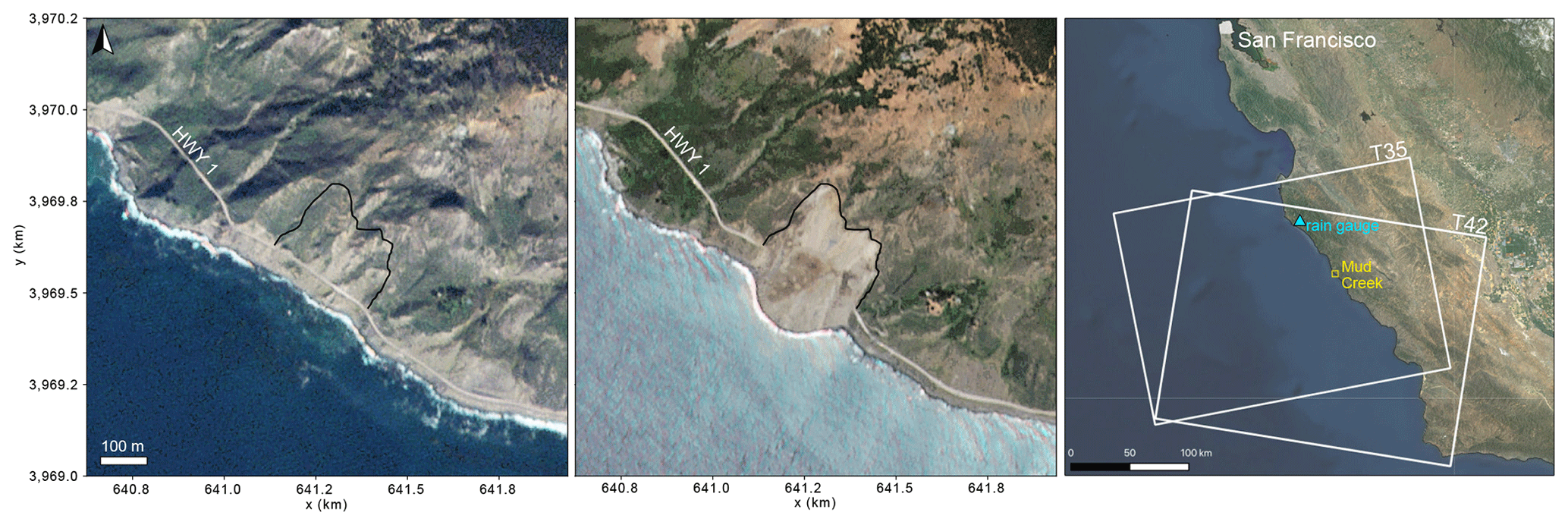
Figure 1 Big Sur coast with Highway 1 before and after the Mud Creek landslide (left and center, x and y coordinates in UTM zone 10 N; images from © Planet Team, 2017), and landslide and rain gauge locations and Sentinel-1 ascending (T35) and descending (T42) orbit footprints (right; basemap from ESRI World Imagery; source: Esri, Maxar, GeoEye, Earthstar Geographics, CNES/Airbus DS, USDA, USGS, AeroGRID, IGN, and the GIS User Community).

Climatically, the Big Sur region experiences a Mediterranean climate. Yearly precipitation averages around 1 m yr⁻¹ and typically falls between November and April. The total yearly precipitation depends strongly on the storm and drought cycles controlled by the El Niño–Southern Oscillation (ENSO). Following a multi-year drought, the winter of 2016/2017 brought an extraordinary number of intense atmospheric-river-driven storms to California, resulting in the state's wettest year on record (Swain et al., 2018).

The Mud Creek slide occurred on 20 May 2017, after 2 weeks of dry weather. The failure initiated at 337 m a.s.l., was 490 m long, and involved roughly 3×10⁶ m³ of earth and rock (Warrick et al., 2019). Prior to failure, the mean slope was 30^∘ (SD = 8.7^∘), with the steepest areas reaching 58^∘. Upon failing, the landslide destroyed almost half a mile (0.8 km) of Highway 1, a vital transportation corridor for both tourism and local residents and the only direct connection between Carmel Highlands on the north end of Big Sur and San Simeon to the south. The landslide potential of this particular stretch of road had become apparent only in the months preceding the slide, as accumulating debris on the road began to require near-daily maintenance (Warrick et al., 2019). Upon recognizing the threat of an imminent landslide, the California Department of Transportation (Caltrans) evacuated all personnel and construction material from the site. Following the catastrophic failure, Caltrans commenced a USD 54 million project to construct a new road over the landslide deposit. The impacted highway segment was reopened on 18 July 2018, more than a year after the slide.

3 Methods and data

For the analyses presented here, we worked with both radar and optical images: we used data from ESA's C-band Sentinel-1A and 1B radar satellites (5.6 cm wavelength) and processed 51 images from the ascending orbit (track 35) and 63 from the descending orbit (track 42). Single Look Complex (SLC) images were obtained from the Alaska Satellite Facility (ASF DAAC: https://search.asf.alaska.edu, last access: 1 February 2021). Because we focused this study on pre-failure landslide dynamics, we did not include any post-landslide radar images in the analysis. To compute the NDVI, we downloaded 22 cloud-free Sentinel-2 images (10 m resolution) from the US Geological Survey's (USGS) Earth Explorer platform (https://earthexplorer.usgs.gov/, last access: 1 February 2021). We used both datasets to compute time series of ratios that describe the discrepancy between the behavior of the landslide and its surrounding slope. The advantage of the ratio calculation is that it cancels out the effects of regional-scale environmental factors and processing artifacts that affect the hillslope and the landslide equally. Therefore, when using the landslide / hillslope ratio, values less than 1 indicate decreasing landslide NDVI or coherence values, while values greater than 1 indicate decreasing hillslope values. Table 1 shows an overview of the raw data products and associated derivatives (details are given in the sections below).

Table 1 Overview of data products used in this study and the number of products derived at the different processing steps.

3.1 Radar background

Two SAR images acquired by the same satellite of a given area at different times can be processed into interferograms: images that represent the phase difference [0, 2π] between the two acquisitions at each point. In the initial interferogram, the phase differences contain contributions from the varying orbital geometries, topography, atmospheric path delays and surface displacements. After removing the effects of viewing geometry, topography and atmosphere, and with knowledge of the radar wavelength, these phase changes can be converted to surface displacements (e.g., Massonnet and Feigl, 1998; Rosen et al., 2000; Wasowski and Bovenga, 2014). Because InSAR is sensitive to deformation only in the instrument's line of sight (LOS), three independent measurements are required to obtain the true 3-D motion of a target. In the absence of independent measurements, LOS deformations can be projected onto the downslope direction by assuming that the primary motion of a landslide follows gravity (see Sect. 3.2.2 and Fig. 4).

Alongside any computed interferogram is a coherence (γ) image that serves as the primary quality indicator for InSAR data. It is a measure of how similar the ground properties are at the time of the radar acquisitions (Scott et al., 2017; Zebker and Villasenor, 1992) and is computed from the local phase variance in the interferogram. Given the stable imaging geometries of Sentinel-1 data, coherence changes are expected to be almost exclusively due to temporal variability. On a vegetated, active landslide, coherence is likely controlled by three factors:

• First, coherence is affected by the surface geometry. The resulting phase of any pixel is the coherent sum of all scatterers within that pixel, and when the geometry of those scatterers changes substantially, the resulting phase changes. Therefore, both changing vegetation and erosion can lead to a loss of coherence (Massonnet and Feigl, 1998; Rosen et al., 2000; Ruescas et al., 2009). In the non-landslide context, this is effect is visible when fields are plowed, crops are harvested or snow falls between two image acquisitions, to name just a few examples.

• Second, displacements that surpass the temporal and/or spatial aliasing thresholds, even if they do not alter the surface geometry, lead to a loss of coherence (e.g., Massonnet and Feigl, 1998; Rocca et al., 2000; Zhou et al., 2009; Wasowski and Bovenga, 2014; Manconi et al., 2018). This effect can be well visible on fast-moving glaciers (e.g., Joughin et al., 1996).

• Lastly, soil moisture may be affecting the coherence, because it can alter radar phase and backscatter. This effect has been shown in many studies, but the reasons are still debated. Soil moisture variations may change the phase response (and backscatter amplitude) by influencing the penetration depth of radar waves, with drier soils allowing deeper penetration. This influences the number of scatterers controlling the phase and backscatter amplitude in any given pixel. Therefore, interferograms created from images with varying soil moisture contents may decorrelate due to the altered number of scatterers. In addition, if soils expand or contract with changing moisture, changing the distance to the radar instrument, the phase response may also be altered, leading to lower coherence (Scott et al., 2017; Rabus et al., 2010; Nolan et al., 2003; Ulaby et al., 1996). Recent studies, however, suggest that coherence loss is better explained by the filling of pore space with water, which increases the dielectric constant, which in turn increases the wavenumber in the soil (Eshqi Molan and Lu, 2020; Zwieback et al., 2015).

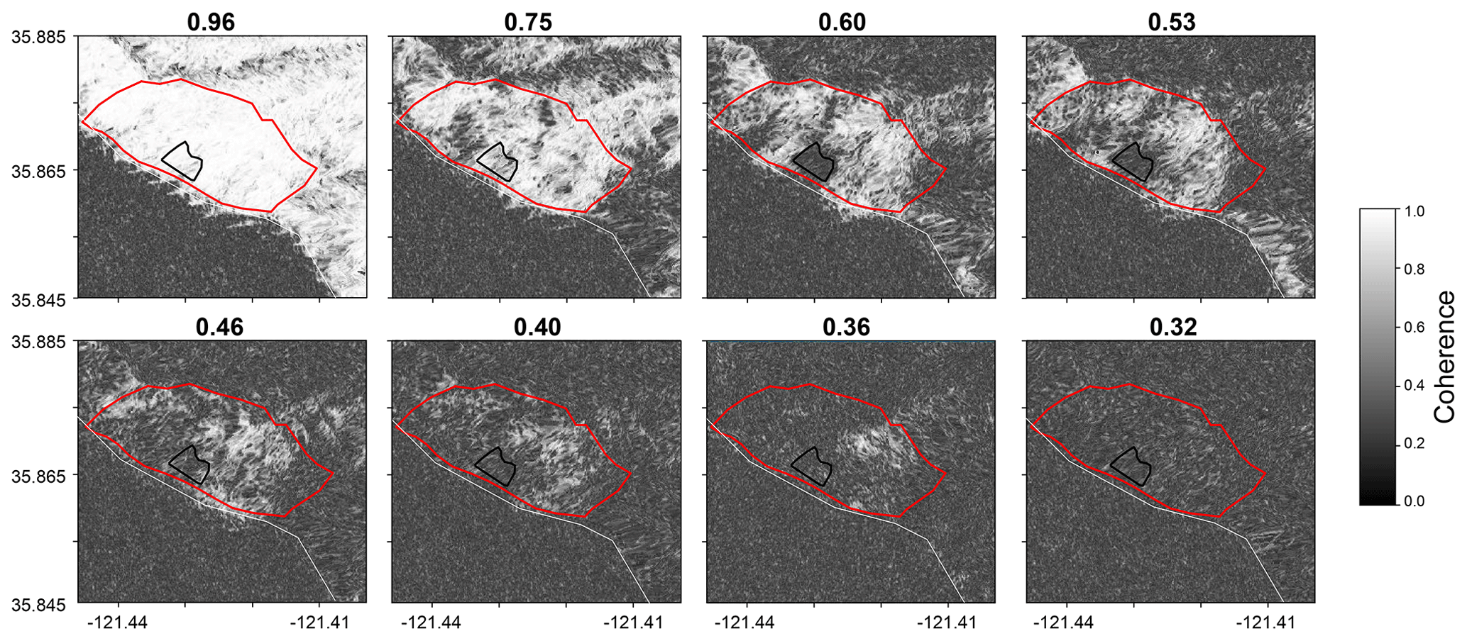
Figure 2 Coherence filtering: interferograms in the upper row exceed the coherence threshold of 0.5 and were therefore included in the ratio analysis; the images in the lower row were excluded. We calculated the mean coherence for the area in the red polygon. The images represent various times during the study period and were chosen purely to show why low-mean-coherence images cannot be used for the ratio calculation. The 20 May 2017 landslide occurred inside the black outline (corresponding to dashed gray line in Fig. 8). Coherence derived from Copernicus Sentinel-1 data.

3.2 Radar processing

We processed the InSAR data using JPL's InSAR Scientific Computing Environment (ISCE; Rosen et al., 2012). SAR images for our study site were available beginning in April 2015, with images typically acquired every 12 d (a few pairs with 6 d spacing were available). We allowed for a maximum time difference of 48 d between images and produced 172 interferograms from the ascending orbit and 208 from the descending orbit (see Table 1). A gap in the ascending data between late 2015 and early 2016 led us to increase the permissible time difference between images in that period to 1 year (maximum resulting temporal baseline = 342 d). Because the study site is relatively small compared to the native spatial resolution of the SAR imagery, we retained a high resolution by only downsampling the images to two looks in range and one look in azimuth. We removed the topographic phase with the USGS's $\mathrm{1}/\mathrm{3}$ arcsec digital elevation model (DEM), the highest-resolution seamless DEM available for the conterminous United States (downloaded from https://viewer.nationalmap.gov/basic/, last access: 1 February 2021). Due to the small size of our area of interest, we did not perform any tropospheric or ionospheric corrections. We unwrapped the interferograms using the Statistical-cost, Network-flow Algorithm for Phase Unwrapping (SNAPHU; Chen and Zebker, 2002) and applied a standard power spectral filter (value 0.5) to reduce the phase noise (Goldstein and Werner, 1998). We subsequently used the generated coherence images and unwrapped interferograms for this study.

Decisions about the quality of an interferogram and the reliability of the data for time series analyses are usually based on radar coherence. For individual interferograms, pixels with a coherence of less than 0.2 are typically masked (e.g., Rosen et al., 2000). Images with low overall coherence are usually omitted from InSAR time series analyses. This selection is often based on visual inspection and performed manually (e.g., Handwerger et al., 2019). To increase the reproducibility of our work, we experimented with a set coherence threshold that we used to filter out poor-quality interferograms. Because our area of interest is small relative to the size of the interferogram, mean image coherence over the entire interferogram is a poor indicator for the data quality in the landslide area. Instead, we calculated the mean coherence for each interferogram within just our area of interest and only retained images with a mean coherence above a defined threshold (0.35 for the displacement analysis and 0.5 for the coherence ratio analysis; see details in Sect. 3.2.1 and 3.2.2). Figure 2 illustrates why relatively aggressive filtering is necessary for the ratio calculations. If the entire area of interest is affected by low coherence, the ratio becomes meaningless. After filtering, we computed the time series of displacement and radar coherence ratio from all the retained images.

3.2.1 Coherence ratio

To construct a time series of coherence evolution, we filtered out all interferograms with mean coherence of less than 0.5 in our area of interest (Fig. 2). This higher threshold was necessary to detect any differences between the unstable part of the slope and the surrounding area. In cases where the coherence of the entire area is low, the ratio value becomes meaningless. We retained 132 interferograms from the ascending track and 141 interferograms from the descending track after applying this filter criterion (Table 1).

ISCE computes coherence using a 5×5 pixel triangular weighted window. For signals s₁ and s₂, coherence is given by

$$\begin{array}{}\text{(1)}& \mathit{\gamma }={\displaystyle \frac{\mid \langle s_{\mathrm{1}}{s}_{\mathrm{2}}^{*}\rangle \mid }{\sqrt{\langle s_{\mathrm{1}}{s}_{\mathrm{1}}^{*}\rangle \langle s_{\mathrm{2}}{s}_{\mathrm{2}}^{*}\rangle }}}\mathrm{0}\le \left|\mathit{\gamma }\right|\le \mathrm{1},\end{array}$$

where ^* indicates the complex conjugate (Jung et al., 2016).

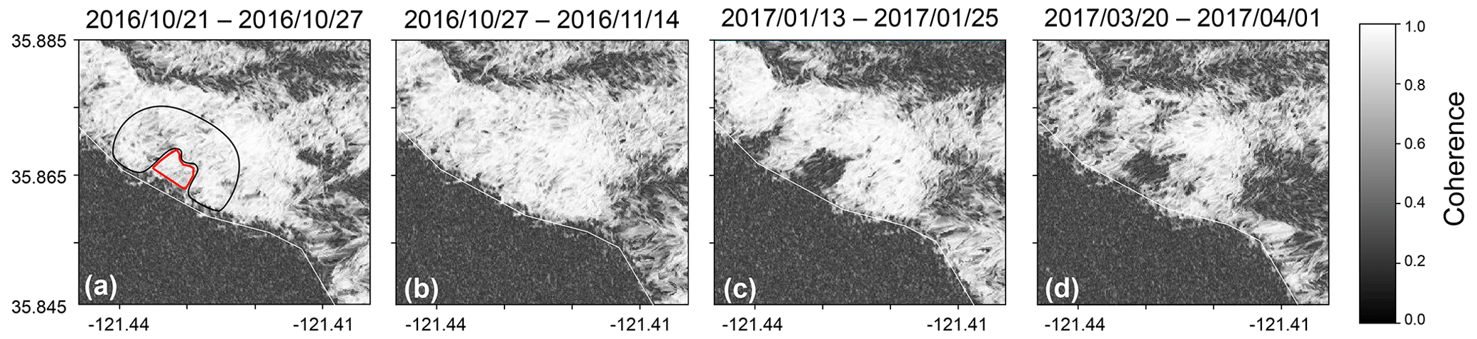
Figure 3 Interferometric coherence of the Mud Creek landslide and surrounding slope in the fall of 2016 (a, b) and spring of 2017 (c, d). The landslide outline is marked in red, and the coherence loss in that area is clearly visible in panels (c) and (d). The reference hillslope is outlined in black. Coherence derived from Copernicus Sentinel-1 data.

We created a time series of radar coherence ratio (C_R) by calculating the ratio between the mean coherence over the slide (the area that ultimately failed) and the mean coherence over the surrounding slope (termed reference slope; see Fig. 3) as

$$\begin{array}{}\text{(2)}& C_{\mathrm{R}}={\displaystyle \frac{{\stackrel{\mathrm{‾}}{\mathit{\gamma }}}_{\mathrm{Slide}}}{{\stackrel{\mathrm{‾}}{\mathit{\gamma }}}_{\mathrm{RefSlope}}}}.\end{array}$$

Figure 3 shows the evolution of the coherence in the area of interest for four interferograms acquired in fall 2016 and spring 2017, as well as the polygons used to calculate the mean coherence on the slide and the surrounding area. For the slide polygon, we mapped the area that failed in the landslide. The reference hillslope was mapped as the area immediately surrounding the landslide with similar slope, aspect and vegetation cover.

3.2.2 Displacement

To complement the coherence ratio time series we also computed a displacement time series. For this part of the analysis, we used only the interferograms from the descending track that had a mean coherence of more than 0.35 in our area of interest. This produced a fully connected time series with 193 interferograms (Table 1). The ascending data do not lend themselves to measuring the displacement because the local incidence angle is around 90^∘, leading to minimal motion in the satellites' line of sight. We selected a point west of the landslide as our stable reference region. This area is the same geologic unit, its vegetation cover is representative of the larger area and it did not fail in the landslide. A preliminary displacement analysis also suggested it had not experienced any significant deformation. We computed the displacement time series using the new small baseline subset (NSBAS; Berardino et al., 2002) method implemented in JPL's Generic InSAR Analysis Toolbox (GIAnT; Agram et al., 2013) and applied a coherence threshold of 0.3 to mask individual low-coherence pixels. We then retrieved surface displacements by projecting the measured line-of-sight deformation at each point onto the fall line. To do this we defined the unit line-of-sight vector a to point from the satellite to the target and the unit fall line b to point from the target downslope along the steepest gradient. We describe both vectors in a polar coordinate system, where θ describes a positive counterclockwise rotation from x (east), and ϕ describes the angle from positive up (Fig. 4). The full slope parallel deformation D_t could then be retrieved as

$$\begin{array}{}\text{(3)}& D_t={\displaystyle \frac{\mathrm{LOS}}{\cos \left(\mathit{\delta }\right)}},\end{array}$$

where LOS is the measured line-of-sight deformation, and δ is the angle between a and b, which is defined as

$$\begin{array}{}\text{(4)}& \cos \left(\mathit{\delta }\right)={\displaystyle \frac{a\cdot b}{\left|a\right|\left|b\right|}}.\end{array}$$

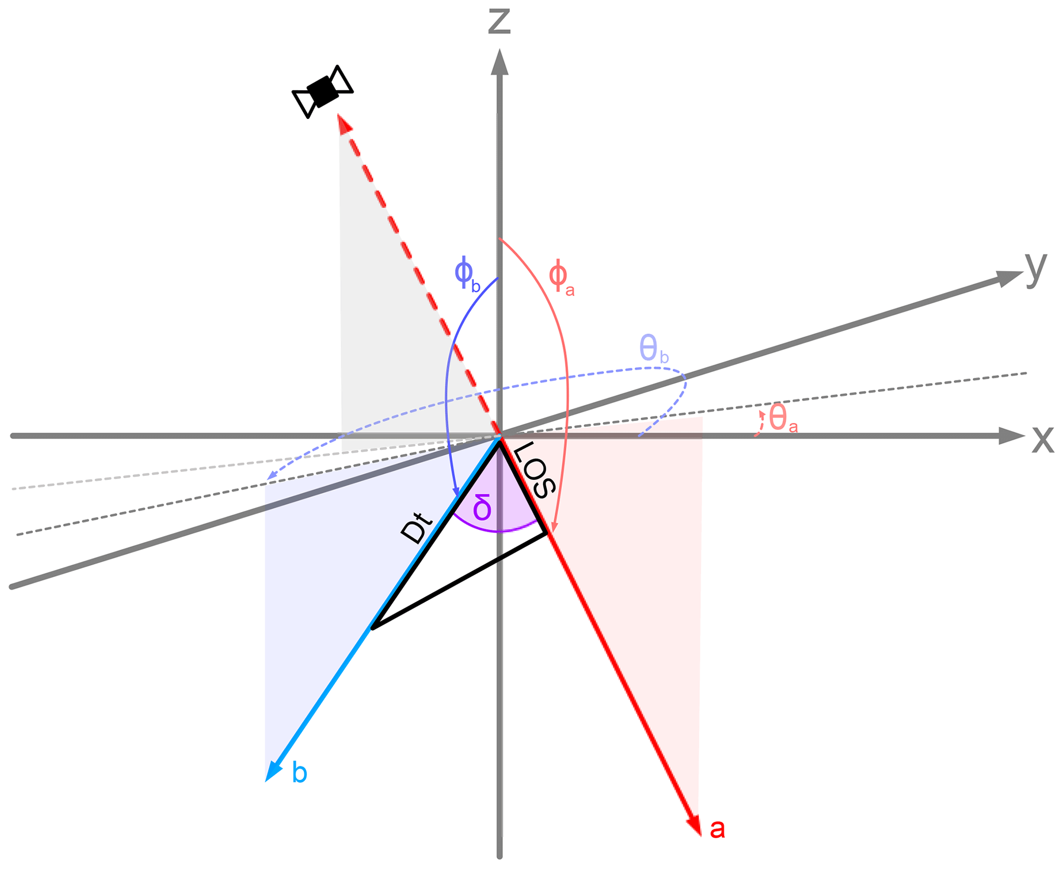
Figure 4 Vector geometries used to project measured line-of-sight displacements (LOS) onto the fall line (b). For a and b, θ describes the azimuth from x (east), and ϕ describes the angle from positive up. The angle δ between a and b controls how much of the true deformation is visible in the satellites LOS.

3.3 Optical data

To investigate the extent to which coherence variability may have been driven by changes in vegetation cover, we computed a time series of the normalized difference vegetation index (NDVI) from 22 ESA Sentinel-2 optical images (Table 1) acquired between 4 December 2015 and 27 May 2017. NDVI is a measure of vegetation productivity that can be derived from the red and near-infrared (NIR) channels in optical imagery (bands 4 and 8 in Sentinel-2):

$$\begin{array}{}\text{(5)}& \mathrm{NDVI}={\displaystyle \frac{\mathrm{NIR}-\mathrm{red}}{\mathrm{NIR}+\mathrm{red}}}.\end{array}$$

NDVI makes use of the fact that photosynthetically active vegetation is bright in the near-infrared spectrum (λ∼800 nm) and dark in the red wavelengths (λ∼600 nm; Tucker, 1979; Carlson and Ripley, 1997). The index values vary between −1 and 1, where denser and/or more productive vegetation results in more positive values, and sparse vegetation or bare ground results in low or negative values. Typical values for dense, healthy vegetation are around 0.6 and values for bare ground or minimal vegetation are typically below 0.2 (Jensen, 2009). We calculated the NDVI for all available cloud-free images back to December 2015 and then computed our time series in the same manner that we did for coherence ratios:

$$\begin{array}{}\text{(6)}& {\mathrm{NDVI}}_{\mathrm{R}}={\displaystyle \frac{{\stackrel{\mathrm{‾}}{\mathrm{NDVI}}}_{\mathrm{Slide}}}{{\stackrel{\mathrm{‾}}{\mathrm{NDVI}}}_{\mathrm{RefSlope}}}}.\end{array}$$

In addition to the time series of the NDVI ratio, we thresholded all NDVI images at a value of 0.25 and investigated the spatial changes through time.

3.4 Precipitation data

Precipitation data were obtained from the National Oceanic and Atmospheric Administration's (NOAA) Global Historical Climate Network Daily (GHCND) platform. GHCND data provide daily total cumulative precipitation and minimum and maximum air temperature. The Big Sur station is located 53 km northwest of Mud Creek at 61 m a.s.l. Data are available from https://www.ncdc.noaa.gov/cdo-web/datasets/GHCND/stations/GHCND:USC00040790/detail (last access: 1 February 2021) and were used without any additional processing.

4 Results

4.1 Coherence ratio

The results of coherence ratio analysis are shown in Fig. 5, alongside the NDVI time series and the precipitation record. The 132 good-quality interferograms from the ascending orbit form a mostly continuous time series, though there was a gap in data acquisition in late 2015 and early 2016. The descending track offers a more continuous time series between 2015 and early 2017 (longest temporal baseline = 48 d), but few interferograms from 2017 passed the coherence threshold. The coherence ratio hovers around 1 throughout the dry seasons in both datasets. In spring 2016, following a short period of intense rainfalls, the coherence ratio calculated from ascending data drops to around 0.8 and only recovers slowly. This drop is less distinct in the descending data. Then, coincident with a large increase in cumulative precipitation in early 2017, the coherence ratio drops markedly to around 0.6 and remains at this level until the catastrophic failure of the landslide.

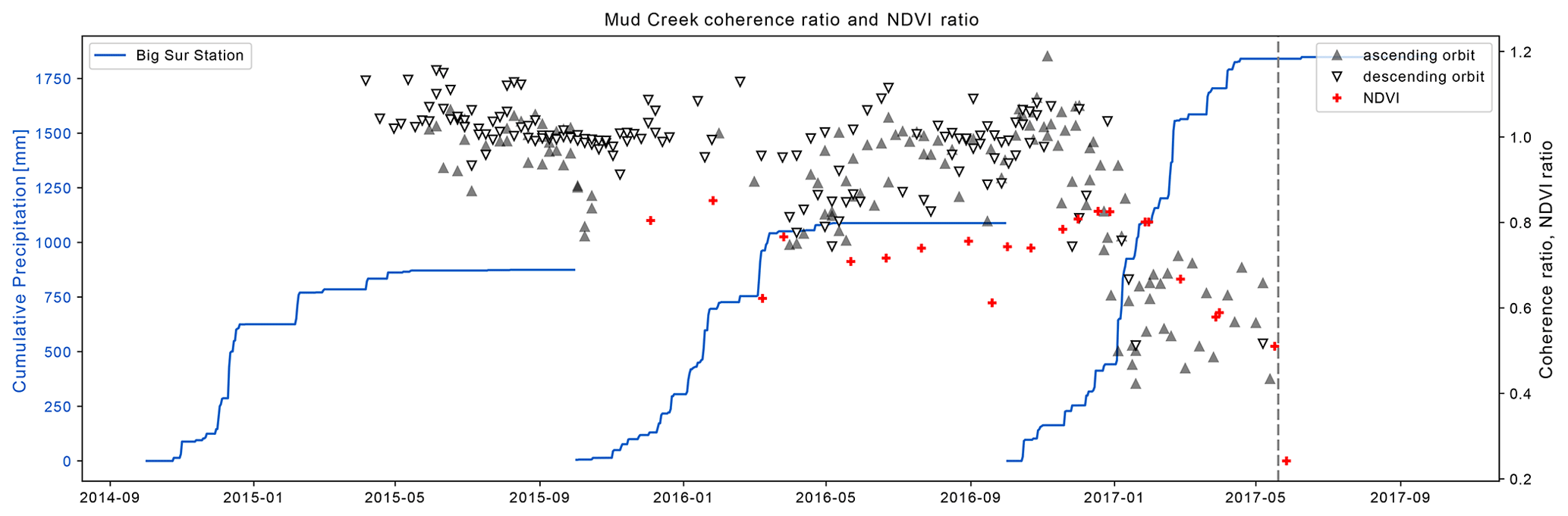
Figure 5 Radar coherence ratio plotted against NDVI ratio and cumulative precipitation (at Big Sur station). The dashed line indicates the timing of the landslide. The coherence ratio hovers around 1 for most of the time prior to the failure, before dropping starkly in January 2017. At the same time, the NDVI ratio begins a gradual decline. A similar behavior for both indices is visible in March 2016.

4.2 NDVI

The NDVI, NDVI ratio and the changes in the spatial pattern also show that processes ongoing on the landslide differed substantially from the surrounding slope. The NDVI ratio of 0.8 prior to 2017 indicates that the Mud Creek slope is generally less densely vegetated than the surrounding hillslope (Fig. 5). This observation is also supported by the raw NDVI time series which indicates that NDVI values on the landslide vary seasonally between around 0.2 and 0.4 while ranging from about 0.25 to 0.5 on the surrounding hillslope (Fig. 6). These individual time series reveal that the evolution of the vegetation cover on the slide closely paralleled that of the surrounding slope throughout 2016, with productivity peaking in April. In early 2017, we observe a clear divergence of the two time series, as vegetation productivity in the slide area began to decline, before plummeting post-slide. These time series demonstrate that the evolution of the NDVI ratio is in fact controlled by a decrease in vegetation productivity or coverage on the slide and not an unusual increase in productivity on the reference slope (Fig. 6). The gradual decline of the NDVI ratio starting in early 2017 therefore suggests that vegetation cover on the landslide was degrading. When comparing this to the spatial evolution of NDVI values, it is evident that low-NDVI regions on the slide were expanding throughout the spring of 2017, driving the decrease in mean NDVI. A low-NDVI area, which can be attributed to a steep gully, is consistently present in the center of the slide (see panel with the typical pattern in Fig. 7). The panel from 8 March in Fig. 7 shows that the drop in NDVI ratio observed in spring 2016 can also be linked to a large expansion of the low-NDVI area (Fig. 5). This drop also corresponded to one of the largest rainfall events witnessed that year. The low NDVI ratio in September 2016 is, on the other hand, caused by a cloud bank obscuring the toe of the slide and is therefore not associated with an actual change of vegetation. Then, throughout the spring of 2017, the low-NDVI area expanded, driving the decreasing mean NDVI until all vegetation was removed due to the failure of the slope (see post-slide image from 27 May 2017 in Fig. 7).

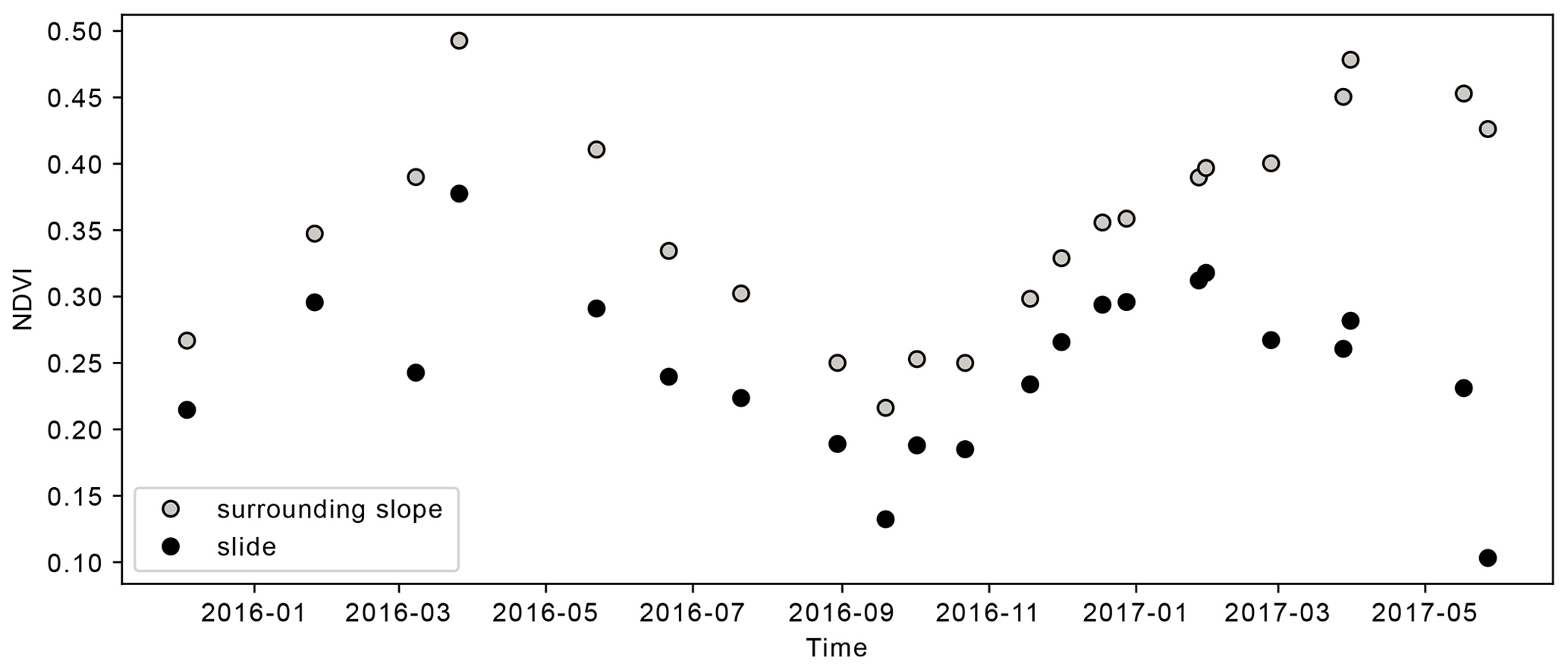
Figure 6 NDVI on the Mud Creek slide body and the surrounding slope. Note that the last data point in May 2017 is from an image acquired after the landslide.

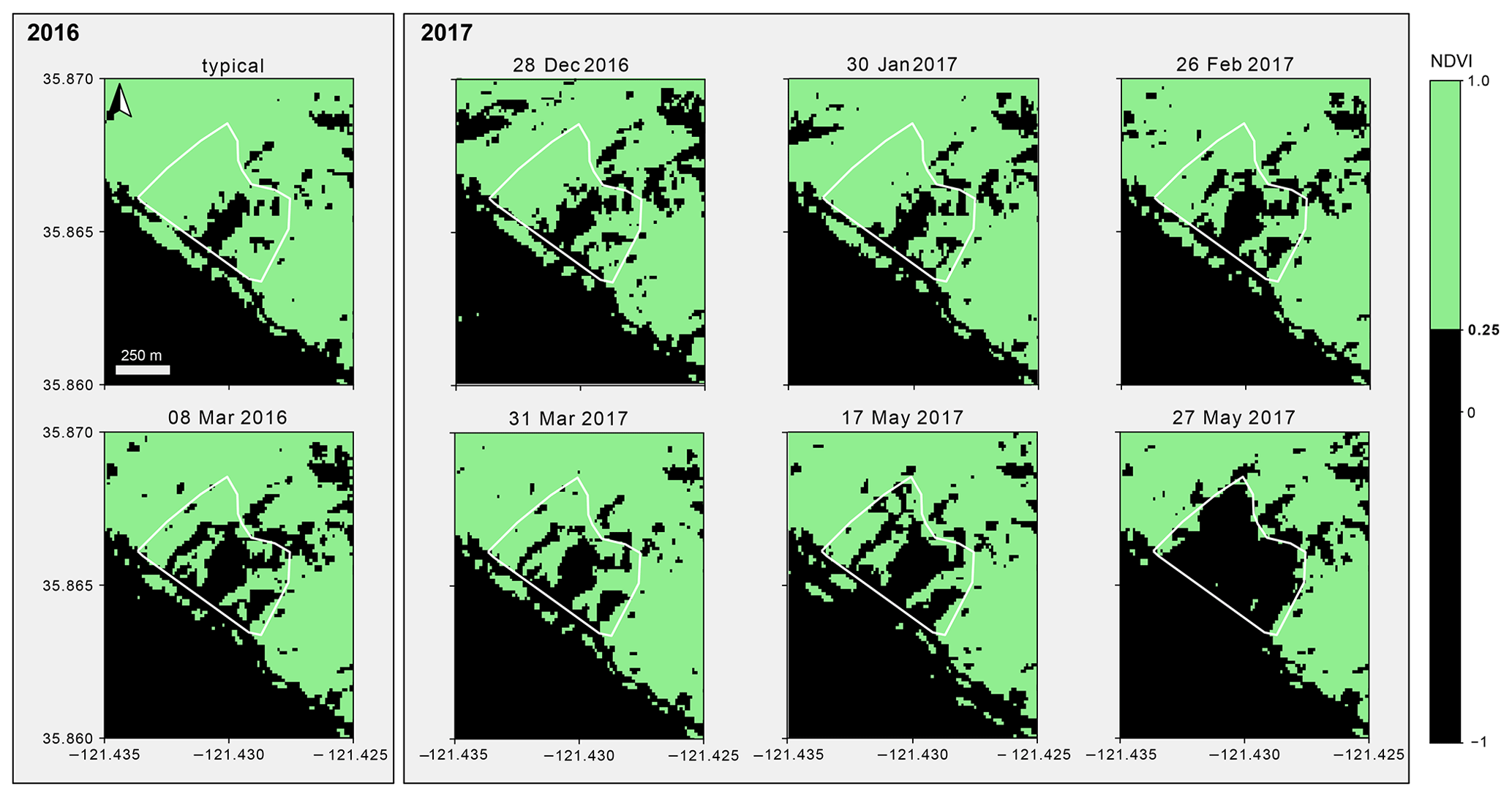
Figure 7 NDVI on the Mud Creek landslide. The first panel shows the pattern that is typical (example from 26 March 2016). The 8 March 2016 panel corresponds to the dip in NDVI ratio visible in early 2016. The area of low NDVI grows ever larger during the spring of 2017, before much of the vegetation is removed during the landslide (post-slide image from 27 May 2017).

4.3 Deformation

On the descending orbit, the line-of-sight intersects the fall line at a favorable angle that allows us to retrieve about 50 % of the total displacement. To retrieve a more accurate record of true deformation we projected the measured line-of-sight displacements onto the downslope direction as described in Eqs. (3) and (4).

Figure 8 shows the slope parallel displacement obtained from the descending track. The total cumulative displacement on the Mud Creek landslide since April 2015 (beginning of Sentinel-1 measurements) ranges from ∼0.15 to ∼0.55 m. The displacement time series at three different points show the large acceleration that took place in spring 2017. The time series from the reference region (solid line in Fig. 8) confirms that the area around the landslide was stable throughout the entire time period. At several points in time, the cumulative displacement reverses direction, indicating that unwrapping errors hamper the retrieval of the true displacement. This behavior is particularly obvious during the 2017 speedup but also during the spring of 2016 (line with stars in Fig. 8). The area showing measurable displacements is somewhat larger than the area that failed on 20 May but smaller than the area that consistently showed low coherence in the months preceding the landslide (dashed lines in Fig. 8).

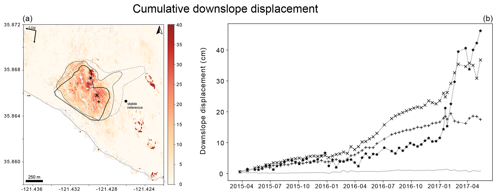
Figure 8 (a) Cumulative line-of-sight displacements from April 2015 to May 2017 projected onto the fall line. The solid black line indicates the extent of the slope that failed, the dashed black line the area showing significant displacement and the dashed gray line the area of low coherence. (b) Time series of displacement at three different points within the slide (indicated by the ★, × and + signs) as well as in the region used as stable reference (solid line).

5 Discussion

Five months before its final failure, in conjunction with some of the largest rainfall events measured during California's 2016/2017 winter season, the coherence ratio over the Mud Creek landslide dropped suddenly. At the same time, the NDVI ratio began a near-linear decline (see Fig. 5). These data raise the question of how and if they can be useful indicators of landslide activity, what challenges this new analysis poses, and what its limitations are.

The fact that fewer interferograms from the descending track passed the coherence threshold can likely be explained by the differences in viewing geometries: the ascending track is right looking, causing the radar waves to intersect the hillslope at a near right angle. Conversely, on the descending track (also right looking), the radar waves intersect the hillslope at an oblique, near-surface-parallel angle. This oblique viewing geometry makes the radar waves more susceptible to volume scattering on vegetation (Massonnet and Feigl, 1998). Indeed, we see widespread areas of low coherence during the growing season in the data from the descending track. Unfortunately, the period leading up to the landslide is most impacted by this effect, while data from the ascending track are much less affected. Despite this discrepancy, the pre-failure coherence drop is visible in the data from both orbits. The coherence loss therefore cannot be attributed to geometric differences but must represent a change on the ground.

The power of the ratio calculation lies in its capability to cancel out negative effects of long temporal baselines, as well as regional atmospheric and environmental changes. If the slope and surrounding hillslope have similar scattering properties, then environmental and atmospheric changes that affect InSAR coherence (e.g., vegetation cycles, precipitation events, ionospheric disturbances) will not differ between a landslide and its surrounding slopes. At Mud Creek, this similarity is given because neither of the slopes are used for agriculture, nor is there any form of human development. Furthermore, both slopes cover a similar altitude range, slope and aspect; optical images suggest they have a very similar vegetation cover (Fig. 1); and the geologic map of the area indicates that the entire area is part of the Franciscan mélange (California Geologic Survey, 2020). In this manner, as long as coherence is maintained in some part of the area of interest, interferograms with varying temporal baselines can be compared to gain insight into governing processes.

The drop of the coherence ratio in the time series is a clear indicator of ongoing changes by itself, but it is useful to consider what factors might be driving these changes in order to understand the value of the coherence ratio with regard to assessing landslide activity. The coherence images (Fig. 3) show clearly that the coherence on the slide dropped drastically; therefore we attribute the effect of the dropping ratio entirely to changing conditions on the slide. However, the change in coherence could be caused by changes to soil moisture, vegetation changes, erosion or active deformation – all of which are processes that may be ongoing on an actively deforming slope that ultimately failed due to increasing pore water pressure (Handwerger et al., 2019). As we try to parse out the different influences on coherence ratio, it is important to note that more than one factor may be the leading cause at any given time, and their relationship may vary through time. Disentangling the causes of the coherence drop is therefore by no means straightforward.

The NDVI ratio began its near-linear decline in the spring of 2017, concurrent with peak precipitation and the observed drop in the coherence ratio. Figure 6 clearly shows that the drop in the NDVI ratio can be attributed to changes that are occurring on the slide and not on the surrounding slope. Indeed, during the spring of 2017, more and more pixels in the slide area showed an NDVI of less than 0.25, indicating that the removal or degradation of healthy vegetation was impacting a larger and larger area. However, the pattern seen on 17 May 2017, just 3 d before the failure, hardly differs from that on 8 March 2016, suggesting that the Mud Creek landslide had experienced this type of vegetation degradation before. Given this similarity, it is likely that the same process led to the low NDVI in 2016 and in 2017. The fact that in 2016 the NDVI ratio recovered within just 18 d (8 to 26 March) suggests that vegetation was not completely removed. If vegetation was not, or only partly, physically removed, covering of plants with mud from ongoing erosion could explain the low NDVI. Whether the vegetation cover was destroyed or just coated in mud, both processes point to an increased activity of the landslide.

The deformation analysis of the Mud Creek landslide shows a significant acceleration prior to failure. However, the displacement time series presented here fails to pick up the period of acceleration in 2016 reported by Handwerger et al. (2019). This is not surprising given that unwrapping errors, the effect of which we see throughout the time series, can make measuring the true surface velocities particularly difficult for fast-moving and accelerating landslides (e.g., Handwerger et al., 2019; Dai et al., 2020; Manconi et al., 2018). Unwrapping errors can be reduced by subtracting the mean landslide velocity prior to the phase unwrapping, which can reveal the missing phase cycles and help recover more of the true deformation (Handwerger et al., 2015, 2019). However, this approach requires assessing each landslide individually and does not lend itself to automatic processing at large scales. We did not apply this correction and are therefore not able to recover the full deformation. Nevertheless, our ∼0.6 m cumulative surface displacement measurements are in good agreement with the ∼0.8 m reported by Handwerger et al. (2019), and the temporal displacement patterns beyond 2016 are nearly identical.

Several factors likely contributed to the changes of the coherence ratio, but we can draw on NDVI and displacement data to discuss what the most likely drivers are and how they relate to landslide activity. In 2016, the NDVI ratio showed a notable drop following the largest rain events that year. This was subsequently followed by a visible drop in the coherence ratio, at least in the data from the ascending track. In 2016, however, the NDVI ratio quickly bounced back, and the coherence also improved again. In 2017, the NDVI continued to decline and the coherence ratio never rebounded. Both the period in 2016 and the one in 2017 were associated with increased displacement. The primary difference between the two periods is that in 2016 the high-precipitation events were limited to a short period, while a series of large magnitude rainfall events occurred throughout the spring of 2017. This suggests that rainfall is inherently linked to the evolution of the NDVI ratio and the coherence ratio. The NDVI patterns show that vegetation cover degraded near-linearly, but we only have a few snapshots in time and cannot reconstruct the immediate responses to increased precipitation. However, both burying vegetation or removing it will alter the surface geometry in such a way that radar coherence is likely reduced. The removal of vegetation decreases root cohesion (e.g., Schmidt et al., 2001), which may have promoted additional surface erosion and also contributed to a change in the slope's scattering processes. The high displacement rates observed in early 2017 can also have contributed to the loss of coherence by overcoming the temporal and spatial aliasing thresholds for displacement measurements.

There is a noteworthy discrepancy between the low-coherence area, the area that exhibits measurable surface displacements and the area that ultimately failed. The area affected by low coherence is by far the largest, suggesting that, since neither vegetation loss nor large displacements were observed in these peripheral areas of the low-coherence region (Fig. 8), soil dielectric property variations are the only remaining factor that may have driven the drop in coherence ratio. This change could be expected to affect the landslide and the stable hillslope similarly, but ultimately the area that failed lay entirely within the low-coherence area. It is not possible to fully disentangle the causes of the coherence drop, but in the landslide context it seems possible that soil moisture changes were more pronounced on this particular part of the hillside, changing the scattering properties of the ground and possibly driving increased surface erosion, vegetation degradation and active slope deformation, which in turn also altered the scattering properties. Combined these changes indicated increased landslide activity and announced the impending failure.

This is, to our knowledge, the first time that coherence ratios and NDVI ratios were used to assess the activity of a landslide prior to its failure. The main advantage of the coherence ratio is that it does not require the computationally expensive unwrapping step in InSAR processing and that it reduces some of the difficulties presented by long temporal baselines. Coupling the coherence ratio analysis with the NDVI ratio links the coherence changes to potential physical changes contributing to the instability. Had the Mud Creek landslide been monitored using these indices, both the 2016 and 2017 drops of the coherence and NDVI ratios could have indicated the increasing landslide activity and prompted the deployment of more precise, possibly ground based, measurements. Given that this study presented the first analysis of this kind, many open questions remain and deserve further investigation.

1. Additional (case) studies are needed to determine which types of landslides may exhibit this kind of behavior and how much deviation from the stable ratios indicates instability. While coherence changes may affect any hillslope, regardless of ground cover, NDVI ratios are not useful in areas that are completely devoid of vegetation (e.g., high-alpine or arctic areas). Since NDVI has a tendency to saturate over very dense vegetation (Lillesand et al., 2015), the limits of this indicator should also be investigated for highly vegetated slopes. Different vegetation indices might be more suitable depending on the situation.

2. Future analyses should determine optimal thresholds for coherence-based filtering thresholds. In order to select the interferograms that contained enough information for the ratio calculation we applied a coherence threshold of 0.5. For simplicity, we chose to apply the same threshold for both the ascending and descending datasets but recognize that this threshold was selected somewhat ambiguously and based purely on visual inspection of the interferograms.

3. A major disadvantage of relying on surface displacements for assessing landslide activity remains the viewing geometry. As in the case of the ascending track at Mud Creek, unsuitable viewing geometries can significantly impede displacement measurements. In contrast, the coherence data from the ascending track – the track that is not well suited to measure surface displacements – provided the more continuous time series of coherence ratio during the spring 2017 acceleration. We stress this fact because radar data affected by layover are frequently deemed unworthy of use in these applications (e.g., Lauknes et al., 2010; Wasowski and Bovenga, 2014; Ohki et al., 2020). The ascending data over Mud Creek are not excessively impacted by this, but the effects are nevertheless visible in the data. Yet the ascending track provides the more useful coherence ratios for this study. Therefore, a systematic analysis of radar coherence may complement traditional InSAR measurements in valuable ways.

4. The separation of the different factors controlling the coherence drop remains somewhat unsatisfactory. Future studies should be aimed at improving this understanding, potentially with the help of polarimetric SAR data that can separate the different scattering mechanisms (Ferro-Famil et al., 2016).

5. We focused solely on the temporal evolution of the ratio between areal mean values, but more insight can likely be gained if investigations are carried out at the pixel or cluster-of-pixels level. This insight could also help identifying what is driving the changes in the mean values.

6. Lastly, in order to perform the ratio calculation, the location and extent of the landslide need to be known beforehand. For now, this limits the current applicability of this indicator to previously identified landslides. However, we believe that intelligent tracking of the behavior of clusters of pixels through time, relative to their surroundings, could be useful for delineating unstable slopes and is worthy of further investigation.

6 Conclusions

Radar coherence has long been used to assess areas of damage after natural catastrophes, but the value of radar coherence or NDVI as possible indicators for impending landslides has not yet been studied. In this study we showed that time series of radar coherence ratio and NDVI ratio may be able to serve as a proxy for landslide activity. Comparatively easy to compute, radar coherence ratios have the potential to be generated at large spatial scales to monitor unstable slopes. In particular, if a few criteria are met, the ratio calculation between the surrounding slope and the landslide eliminates interference due to temporal coherence loss, atmospheric disturbances or vegetation cycles. Our analysis also indicates that this type of analysis can fill data gaps in places where data from only one orbit are suitable for deformation measurements. Nevertheless, questions around whether it is possible to fully disentangle the different factors leading to the pre-failure coherence loss and how common this kind of signal is for different kinds of landslides remain to be resolved. Similarly, it is worth investigating how the presence of more or less vegetation and use of different radar wavelengths influence the results. We also believe that it could be possible to automatically identify drastic drops in radar coherence ratios and NDVI ratio decreases, suggesting that this tool could be used to identify impending failures. All things considered, we strongly believe that the encouraging initial results presented here motivate further investigations of these parameters.