the Creative Commons Attribution 4.0 License.
the Creative Commons Attribution 4.0 License.
 | 03 Dec 2021
Applying machine learning for drought prediction in a perfect model framework using data from a large ensemble of climate simulations
Ralf Ludwig
There is a strong scientific and social interest in understanding the factors leading to extreme events in order to improve the management of risks associated with hazards like droughts. In this study, artificial neural networks are applied to predict the occurrence of a drought in two contrasting European domains, Munich and Lisbon, with a lead time of 1 month. The approach takes into account a list of 28 atmospheric and soil variables as input parameters from a single-model initial-condition large ensemble (CRCM5-LE). The data were produced in the context of the ClimEx project by Ouranos, with the Canadian Regional Climate Model (CRCM5) driven by 50 members of the Canadian Earth System Model (CanESM2). Drought occurrence is defined using the standardized precipitation index. The best-performing machine learning algorithms manage to obtain a correct classification of drought or no drought for a lead time of 1 month for around 55 %–57 % of the events of each class for both domains. Explainable AI methods like SHapley Additive exPlanations (SHAP) are applied to understand the trained algorithms better. Variables like the North Atlantic Oscillation index and air pressure 1 month before the event prove essential for the prediction. The study shows that seasonality strongly influences the performance of drought prediction, especially for the Lisbon domain.
- Article
(1786 KB) - Full-text XML
- BibTeX
- EndNote


Droughts remain to be one of the most dangerous hazards, having a serious and large-scale impact on environment, society and economy. Recent events like the summer 2018 drought in huge parts of central Europe led to severe forest fires and crop failures. The damage was estimated to amount to several hundred millions of euros solely in Germany (Federal Ministry of Food and Agriculture, 2018). Moreover the effect of global warming leads to major changes in the earth's climate system, having a direct influence on the frequency and severity of extreme events like droughts (Spinoni et al., 2016). An increase in frequency of drought occurrence is a major threat for current and future generations, and comprehensive knowledge on the phenomenon of drought is needed in order to take action early and to prevent humanitarian catastrophes. This goes in conjunction with drought prediction. Precise drought prediction would enable the mitigation of the dangers connected to drought occurrences such that stakeholders, for example, would be able to store the maximal possible amount of water in the endangered regions. This would help to mitigate the water shortage when the drought arrives. Measures for demand reduction like that could be introduced earlier and to a better-adjusted extent; this would help to reduce the economic and societal damage.
To mitigate the effects of droughts the information on the their onset is of crucial importance. This can be derived from a drought index. A variety of drought indices exist, which are typically defined according to statistical and physical measures. These mostly take into account atmospheric and soil variables. Among the most popular ones are the standardized precipitation index (SPI), standardized precipitation evaporation index (SPEI), soil moisture percentile (SMP) and Palmer drought severity index (PDSI). The standardized precipitation index (SPI) is adopted as the standard meteorological index by World Meteorological Organization (2012). It is a measure of meteorological drought based on the probability of occurrence of certain precipitation amounts in the area of interest (Sheffield and Wood, 2011). Studies on drought prediction by Belayneh et al. (2016) and Bonaccorso et al. (2015) use SPI as a prediction variable for the forecast.
Forecasting of any physical phenomenon can be done by either a physical, conceptual or data-driven model. The latter ones are widely used due to their rapid development times and the flexibility in input parameters. McGovern et al. (2017) argue that AI methods have a high potential for prediction of extremes due to the ability of machine learning methods to learn from past data, to handle large numbers of input variables, to integrate physical understanding into the models and to discover additional knowledge from the data.
A review of seasonal drought prediction given by Hao et al. (2018) identifies two typical predictor groups of variables: large-scale climate indices that reflect the atmosphere–ocean circulation patterns and local climate variables. The first ones are known to correlate with precipitation patterns in special regions and therefore are naturally correlated with the occurrence of drought. The teleconnection indices important for European precipitation include North Atlantic Oscillation (NAO), Scandinavian Oscillation (SCA), East Atlantic–Western Russia Oscillation (EAWR), East Atlantic Oscillation (EA) and Atlantic Multidecadal Oscillation (AMO) (Hao et al., 2018). As shown by Folland et al. (2009) a positive NAO index in summer is associated with dry and warm conditions in the northwest of Europe, whereas southern Europe and the Mediterranean experience cooler and wetter conditions. More information on the influence of the NAO, SCA, EA and EAWR on the European climate can be found in Folland et al. (2009), Bueh and Nakamura (2007), Mikhailova and Yurovsky (2016), Lim (2015); Barnston and Livezey (1987) and Sheffield et al. (2009). A positive phase of AMO is associated with humid conditions over Great Britain and parts of Scandinavia and with dry conditions in the Mediterranean (Sheffield and Wood, 2011, p. 26); the negative phase is associated with a reversed pattern: dry conditions in Great Britain and wet conditions in the Mediterranean. A study by Sheffield et al. (2009) showed a correlation between the amount of droughts and AMO of 62 % with a significance at the 90 % level. A recent study by Bonaccorso et al. (2015) uses NAO for prediction of probability of drought occurrence for Sicily. The local climate variables like precipitation, temperature and soil moisture were also used as inputs to reflect the conditions at the time the prediction occurs. Belayneh et al. (2016) and Bonaccorso et al. (2015) used SPI for the past months as input variable to the algorithm. A study by Morid et al. (2007) used precipitation as an input parameter.
This paper examines the possibilities of meteorological drought prediction with the lead time of 1 month, applying artificial neural networks (ANNs) for two domains with different climate: one with Mediterranean (Lisbon) and one with continental climate (Munich) (Ceglar et al., 2019). Both sites experienced an increase in drought frequency when comparing 2015 and 1950 and are projected to keep rising under RCP4.5 as well as RCP8.5. (Spinoni et al., 2017). Observational data offer only a limited field for drought investigation, as can be seen from the following approximation. Systematical weather observations started in 1781 by the Societas Meteorologica Palatina (Kington, 1980). In this study is used as a threshold for drought occurrence. It corresponds to the 15 % driest months (Keyantash and National Center for Atmospheric Research Staff, 2018) and can be estimated by a total number of 430 observed events until the year 2020 (Eq. 1).
Compared to that, CRCM5-LE offers a total number of roughly 4500 events when using the first 50 years from the climate simulation data (1955–2005) (see Eq. 2).
This is a difference of an order of magnitude. The more data are available the better the predictions that can be derived by a drought-predicting machine learning model and the more can be learned about drought formation. According to von Trentini et al. (2020) precipitation in summer and winter derived from the European gridded dataset (E-OBS) does fall to a high percentage into the range produced by CRCM5-LE for the historic period. Therefore, the CRCM5-LE proves applicable to this study, and its larger number of extreme events can be used as input to the machine learning algorithms. In this study a variety of ANNs are trained. The best-performing models are investigated, using explainable AI methods to understand the results.
While no comparable study exists for the Munich domain, Santos et al. (2014) performed a drought prediction based on SPI6 for Portugal for the months April, May and June using the following input variables: sea surface temperatures (JFM), NAO (DJFM) and cumulative precipitation (NDJFM for SPI6April, DJFM for SPI6May, JFM for SPI6June). The best results were achieved for the prediction of SPI6 for April, with a correlation coefficient of 0.98. SPI6 for May and June referred to a correlation coefficient of 0.78 and 0.77, respectively.
2.1 Datasets
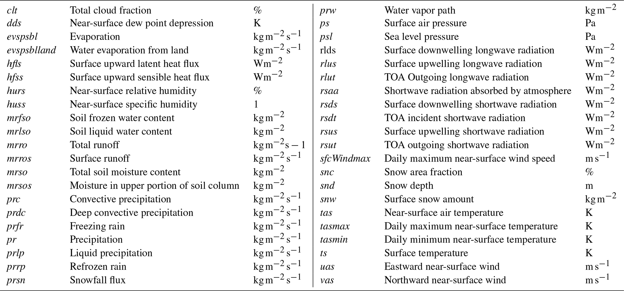
To investigate the predictability of drought data from the single-model initial-condition large ensemble (SMILE) consisting of 50 members, the Canadian Regional Climate Model 5 Large Ensemble (CRCM5-LE) is used. The data were produced within the scope of the ClimEx project (Leduc et al., 2019, http://www.climex-project.org, last access: 28 November 2021). The CRCM5-LE was generated by dynamical downscaling of the data provided by the 50-member initial-condition Canadian Earth System Model 2 using the Canadian Regional Climate Model 5 (Martynov et al., 2013). The data have a resolution of 0.11∘ (12 km) and are produced for the years 1950–2099 for a European and an eastern North America domain. For the years 1950–2005 the historical greenhouse gas concentrations and aerosol emissions are being used. Starting from 2005, the model introduces the RCP8.5 (IPCC, 2013) forcing scenario. A total of 42 atmospheric variables are available at a temporal resolution of 1 to 3 h. They are used on a monthly basis as input to the machine learning algorithms. The list of variables is provided in Table 1.
Table 1The 42 monthly atmospheric and soil variables from CRCM5-LE. TOA refers to top of atmosphere.
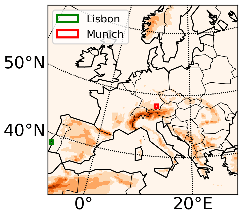
In the study we use monthly sea level pressure (psl) from the driving model CanESM2-LE (Kushner et al., 2018; Kirchmeier-Young et al., 2016) for the calculation of North Atlantic Oscillation (NAO), Scandinavian Oscillation (SCA), East Atlantic Oscillation (EA) and East Atlantic–Western Russia Oscillation (EAWR) over the whole Atlantic basin (20–80∘ N, 90∘ W–40∘ E). The Atlantic Multidecadal Oscillation (AMO) is calculated using the sea surface temperature (SST) over 0–60∘ N, 0–80∘ W from the CanESM2. Only the period 1955–2005 is considered in order to stay within the scope of historical climate. The CRCM5 domain is displayed in Fig. 1. For the machine learning training a grid point situated at 48.11∘ N, 11.91∘ E is referenced as Munich, and 38.67∘ N, 9.17∘ W is referenced as Lisbon.
2.2 Input variables for drought prediction
In order to calculate NAO, SCA, EA and EAWR, the method introduced by Hurrell et al. (2003) is used: a principal component analysis (PCA) of the monthly psl is performed over the 20–80∘ N, 90∘ W–40∘ E domain. The leading eigenvectors, scaled by the amount of variance they explain, represent the leading circulation patterns of the atmospheric system. The first eigenvector corresponds to NAO, the second one to SCA, the third one to EA and the fourth one to EAWR. To calculate the teleconnection indices (NAO, SCA, EA, EAWR) the eofs package described in Dawson (2016) is used. It is an implementation of the technique of empirical orthogonal functions (EOFs) (Dawson, 2016). The leading modes of the PCA corresponding to NAO, SCA, EA and EAWR derived from the CanEsm2 dataset are shown in Fig. 2.
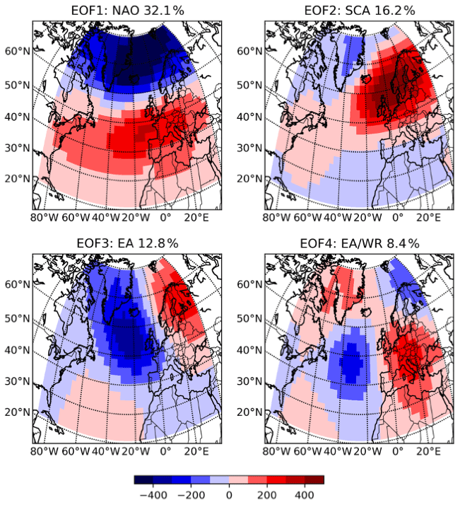
Figure 2First four leading eigenfunctions of the mean sea level pressure in CanESM2. Percentage of variance the mode explains is given at the top of the panels.
AMO is calculated by spatial averaging over the 0–60∘ N, 0–80∘ W area of the anomaly of sea surface temperature (Trenberth, 2011). Additionally the 10-year running mean of AMO is calculated as an input variable as it is widely used in various studies and was shown to be correlated with precipitation (Enfield et al., 2001).
Variable subset selection helps to limit the computational time and to improve predictive accuracy (Kumar and Minz, 2014). In order to eliminate redundant variables, Pearson's R between all the CRCM5 variables for the chosen domains is calculated. Pearson's R (ρX,Y) is a measure of linear correlation between two variables X and Y; ρX,Y equals 1 if the correlation is totally positive, 0 if there is no linear correlation and −1 if the correlation is total negative (Guyon and Elisseeff, 2003). For two samples x and y, Pearson's R is defined in the following way:
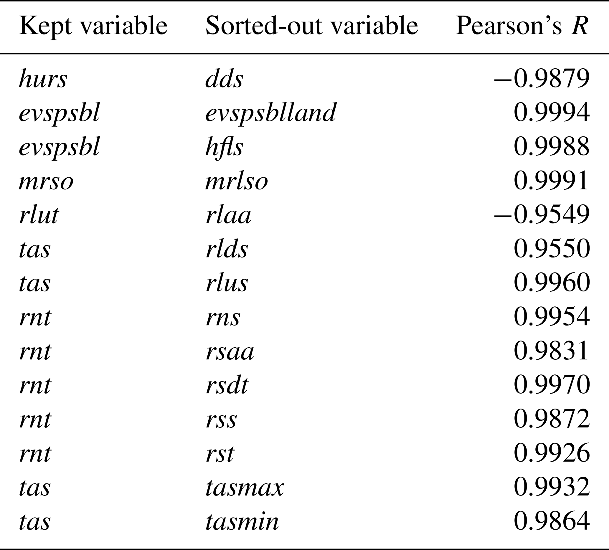
The bar refers to the average over the index i (Guyon and Elisseeff, 2003). Pearson's R is a popular and easy method for feature selection of continuous variables as introduced in Biesiada and Duch (2007); ρ is calculated for all possible permutations of the 41 input variables. The ones correlating to a high degree are examined, and a threshold of 0.95 is chosen. In Table 2 a list of sorted-out variables and the corresponding values of Pearson's R is given. The high correlation values can be explained by a physical relationship between the variables: e.g., the total evaporation (evspsbl) is almost the same as evaporation from land (evspsblland) as there are no relevant water bodies in the chosen domains. Out of the full list of 42 variables, 14 are sorted out as being redundant.
2.3 Standardized precipitation index
The standardized precipitation index (SPI) is a precipitation-based index introduced by McKee et al. (1993). For the calculation of SPI a continuous monthly precipitation dataset is used. The index can be calculated on different timescales: typically, it is 1, 3, 6, 12 or 24 months. As a first step the precipitation values are accumulated for the needed timescale. The resulting dataset is fitted to a gamma distribution for each month separately and then transformed to a normal distribution such that the mean SPI is zero. The SPI value for a given precipitation is then the number of standard deviations from normal. Because of the normalization, the SPI is especially useful to represent wetter and drier climates as well as to account for differences among seasons. As the two study sites are having different meteorological conditions, the SPI provides a convenient and comparable measure (Zargar et al., 2011). As noted in Yoon et al. (2012) the accumulation period of the SPI value needs to be chosen equal to or less than the prediction lead time as otherwise the precipitation values needed for the mathematical calculation of the SPI would be given as input to the machine learning algorithm. Therefore the accumulation period of 1 month is chosen. SPI1 is calculated for Lisbon and Munich each using the data from 1955–2005 from all members as reference.
2.4 Machine learning
This study investigates drought predictability applying the technique of supervised machine learning for this purpose. Machine learning is a promising tool for the analysis of complex and data-rich phenomena as droughts (McGovern et al., 2017). The Python package Keras, a high-level neural network package, is used for the design of the machine learning models (Chollet et al., 2015) as it allows the design of neural networks in an easy way by adding layers. Three crucial elements are needed to perform drought prediction by supervised machine learning: input data; a target variable to be predicted; and a computation pipeline, which includes the machine learning algorithm.
The data from the years 1957–1999 are used as training data; the years 2000–2005 are used for the testing purpose. Each of the time periods is available 50 times as we are dealing with an ensemble of 50 members. This results in 2150 model years for training and 250 years for testing. A small fraction of the training data are used for the validation of the machine learning algorithms. The target variable chosen for the prediction of droughts is SPI1. Two classes for the prediction are identified in the following way: is defined as an event and is initialized with 1; is initialized with 0 and corresponds to a non-drought event. The lead time of 1 month is chosen for the prediction as it has been used in previous studies by Yoon et al. (2012) and Deo et al. (2017). Moreover shorter prediction lead times usually obtain better results when compared to longer periods, as seen in Bonaccorso et al. (2015). After the feature selection 28 variables originating directly from the CRCM5-LE dataset are used as input. In addition to those the teleconnection indices NAO, SCA, EA, EAWR, AMO and AMO10 are used as input.
To predict, for example, a drought or non-drought in April of 1980, the data for 12 months before the event are used as input. This is NAO and other teleconnection and atmospheric variables for the period April 1989–March 1980; for a prediction of an event in May 1980, May 1989–April 1980 is used as input. The 12 months before the event are chosen in accordance with the study by Morid et al. (2007), who found that the best-performing drought prediction model was the one including the value up to 12 months before the predicted one. We perform a time series prediction with no limitation on special months or seasons to be inspected.
For this analysis we use a supervised machine learning algorithm, an artificial neural network (ANN). ANNs are algorithms whose design is inspired by the architecture of the human brain with its neurons (Russell and Norvig, 2009); they both consists of connected nodes. A link between the node i and the node j serves to propagate the activation ai from i to j. To each connection a numeric weight wi,j is assigned. The output of the node is computed by
(Russell and Norvig, 2009, p. 728). The activation function defines the output of the node. In order to have stable learners with confident predictions a function with a soft threshold is recommended (Russell and Norvig, 2009). In this study the following three activation functions are used: sigmoid, rectified linear unit (ReLU), exponential linear unit (ELU). Sigmoid activation is especially useful for the output layer (Russell and Norvig, 2009), while ReLU and ELU both have the property of allowing very fast optimization (Maas, 2013).
The sigmoid function, also called the logistic function, is defined in the following way:
(Russell and Norvig, 2009). This function has an output between 0 and 1. This can be interpreted as a probability of belonging to the class 1. One of the main disadvantages of the sigmoid activation function is the vanishing gradient problem: at higher, almost saturated layers with values of 1 or −1, the gradients become nearly 0, resulting in a slow optimization convergence (Russell and Norvig, 2009, p. 726).
ReLU refers to rectified linear unit and shows better performance when dealing with the vanishing gradient problem (Maas, 2013). ReLU is defined in the following way:
ELU refers to the exponential linear unit and was introduced by Clevert et al. (2016). Clevert et al. (2016) claim that in experiments the ELU activation led to faster learning and significantly better generalization performance than ReLU and sigmoid activation. The function is defined as
α controls the value to which an ELU saturates for negative inputs. Per default the value is set to 1 such that the function saturates at −1.
Two kinds of layers are used in this study: dense and dropout. Dense refers to a regular fully connected neural network layer. Dropout refers to a layer which is randomly setting a fraction of inputs to zero at each update. This technique is used to prevent overfitting and therefore to improve the performance of the algorithm (Chollet et al., 2015). The first part of the study concentrates on the methodological search for the best-performing algorithms. A pipeline to search for the best-performing architecture, value for L2 regularization and loss function is built up.
The model performance is evaluated using accuracy and F1 score (Sasaki, 2007). The latter one is especially useful when training on datasets with an imbalanced class distribution as it is in the case of our dataset. Accuracy is defined in the following way:
F1 score is a harmonic measure between precision and recall. Precision is the amount of true positives with respect to the amount of positively classified data. Recall is the amount of true positives with respect to the total number of positives in the data. The F1 score is defined in the following way:
Due to the class imbalance within the dataset we require that the accuracy of each class is at least 50 %. In that case given the distribution of the test dataset of 1803 non-drought events to 387 droughts for Lisbon and 1848 non-drought events to 352 drought events for Munich a marginal F1 score of 0.26 for Lisbon and 0.24 for Munich is given.
The best-performing models are additionally evaluated using the Heidke skill score (HSS). The range of the HSS is −∞ to 1. Values below zero indicate that the random forecast (a forecast which randomly assigns the labels) has a better performance than the trained model. HSS of 1 indicates a perfect forecast. HSS is defined in the following way:
where a is the number of true positives, b the number of false positives, c number of false negatives and d number of true negatives.
The second part of the study analyzes the best-performing algorithms (one for the Lisbon domain, one for the Munich domain) by applying explainable AI methods. SHAP (SHapley Additive exPlanations) is a state-of-the-art method for interpretation of machine learning models, which was inspired by game theory (Lundberg and Lee, 2017). It estimates for each input feature an average marginal contribution to the prediction of the result and therefore allows a comparison of the contributions among different features. In addition to that the difference in predictability among the seasons is calculated and compared to gain a better understanding on the influence of seasonal weather patterns.
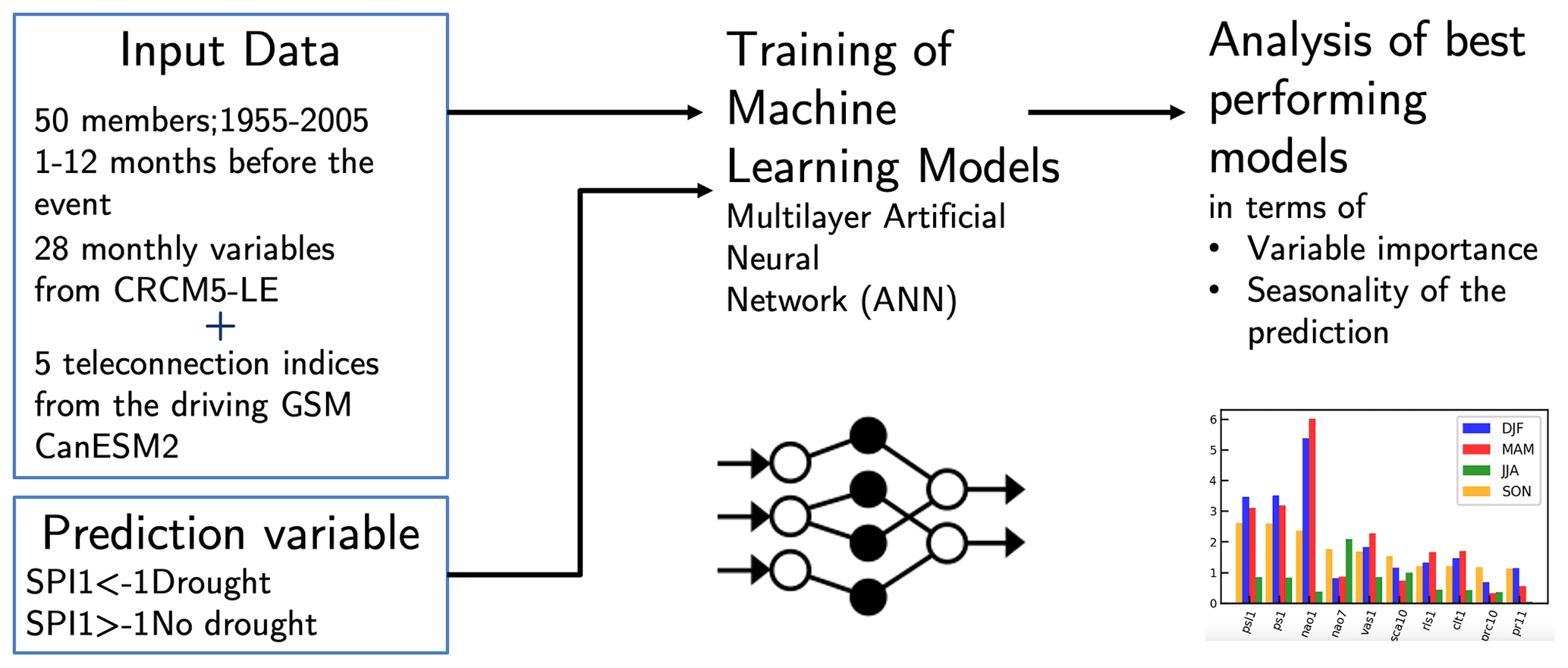
An overview of the proposed methodology can be found in Fig. 3.
This study consists of two parts: the first part deals with a systematical search for the best-performing setup of the ANN model for the two domains of interest: Munich and Lisbon. A repeated training is conducted by varying the values of parameters like the architecture of the hidden layers, L2 regularization and the loss function. In the second part of the analysis the best-performing models for the two domains are analyzed using explainable AI methods.
3.1 Model training results
For the design of the ANN it is crucial to perform fine-tuning of the model parameters to find the optimal setup. An architecture has to have enough layers and neurons to capture the complexity of the dataset (Goodfellow et al., 2016). In order to find the best architecture the learning curve of the algorithm is inspected. The learning curve shows the loss of the training and validation datasets on the weights during the training (Goodfellow et al., 2016). Two examples are shown in Fig. 4. The plot shown at the top refers to an architecture which is not able to capture the complexity of the dataset: the loss is hardly decreasing in the training or validation data. The bottom figure refers to an architecture which overfits: in the last epochs the loss of the validation dataset is rising, while it decreases in the training dataset.
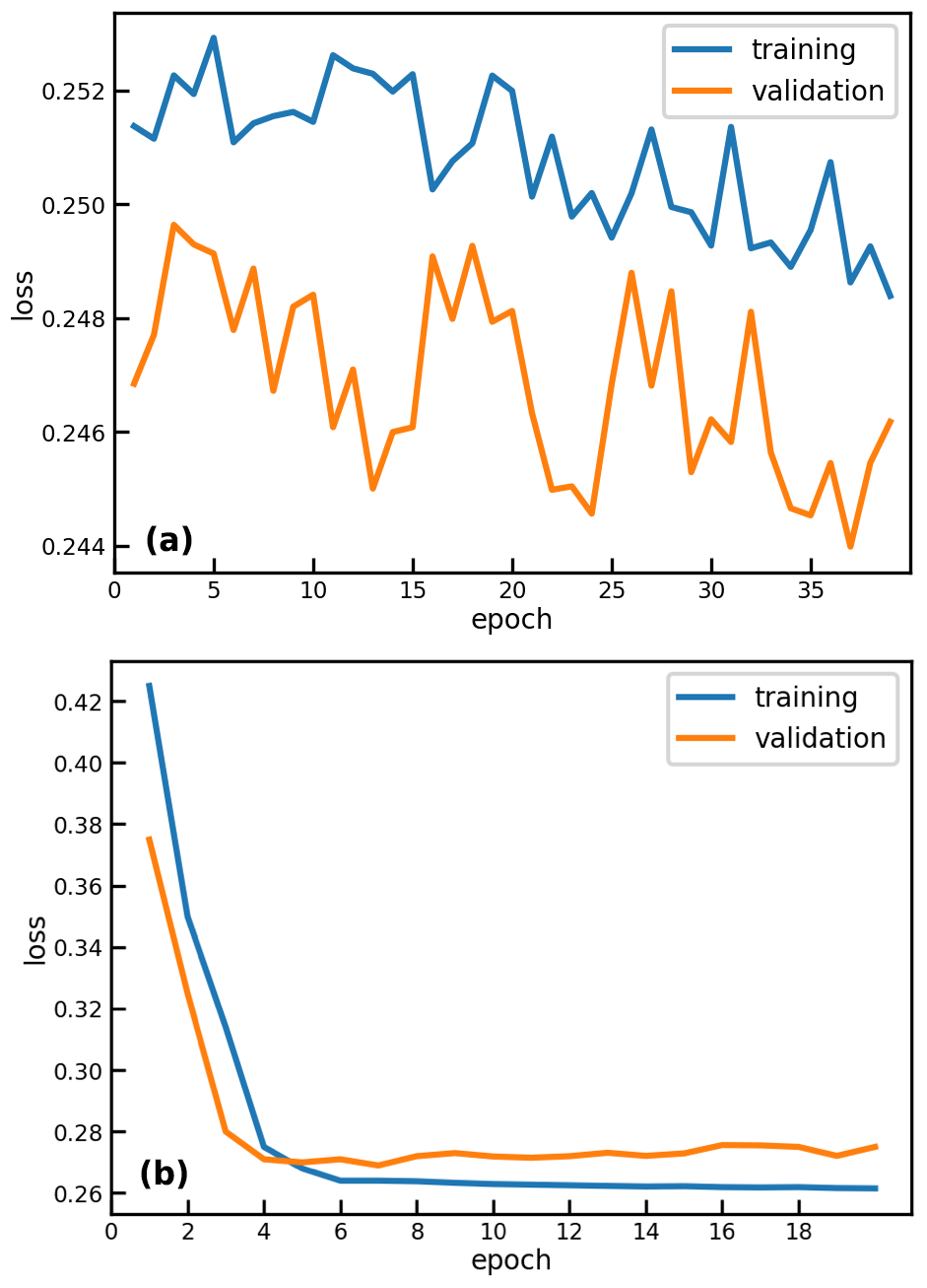
Figure 4Learning curve for two chosen fitting examples: algorithm complexity insufficient (a) and overfitting (b).
In this way a network is searched which captures the given complexity of the dataset. This is reached with an algorithm consisting of at least five layers. Additionally two dropout layers, which set a specified number of nodes to zero in a random way, are introduced in order to fight overfitting.
3.1.1 L2 regularization
L2 regularization is a broadly applied method to prevent overfitting in the training data (Bishop, 2007). The main idea behind regularization is to add a penalty term to the loss function, which will punish the classifier for complexity and force some of the weights to zero (Russell and Norvig, 2009). In case of L2 regularization the punishing term is proportional to the L2 norm of the weight vector. The weight of the punishing term λ determines the relative importance of the regularization.
Table 3Results of ANN training for different values for λ for L2 regularization. λ of 0.001 (bold) is chosen for both domains for subsequent training since the performance of the model with regards to the F1 score has a higher importance for an imbalanced dataset than the pure accuracy.
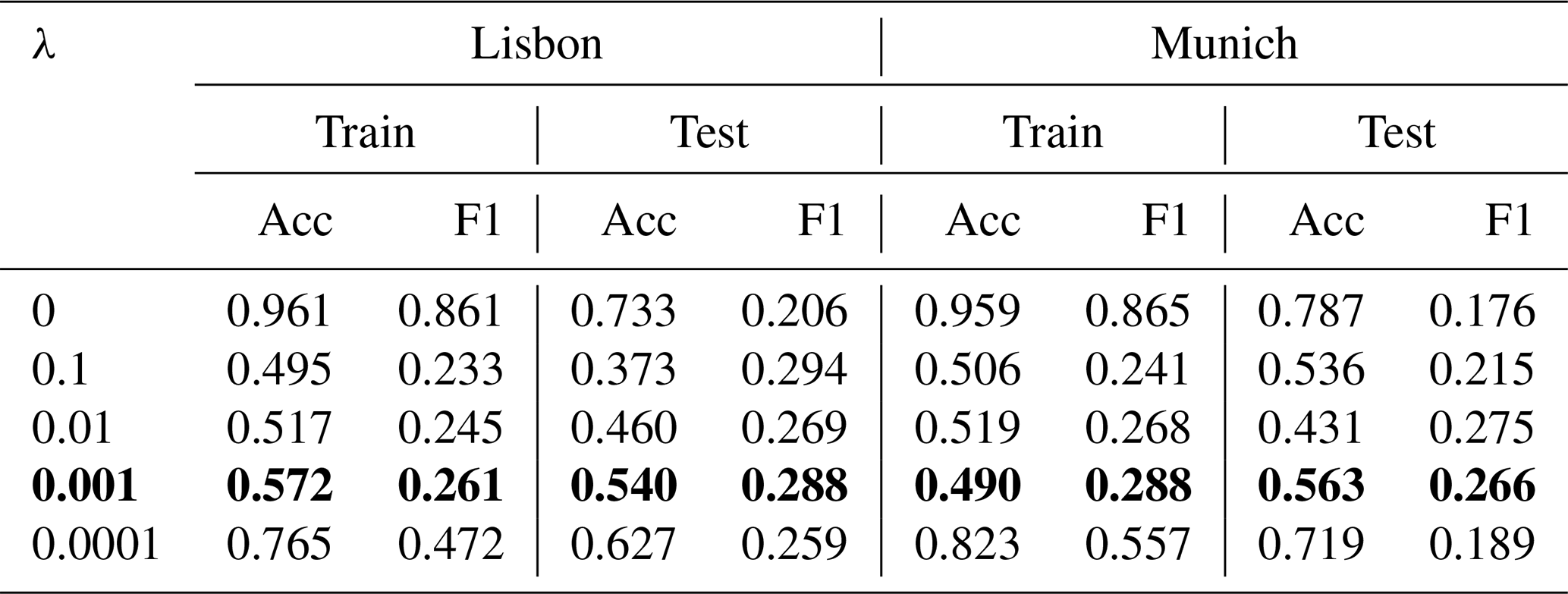
The results of the training with different values of λ for L2 regularization are shown in Table 3. Training results are displayed in this particular case as the regularization is introduced to prevent overfitting. Generally the performance for the test dataset is more important and will be inspected in following experiments. If λ is set to zero the regularization term vanishes. Especially in those cases the overfitting is high. For Lisbon overall higher performance could be seen for λ values around 0.01, 0.001 or 0.0001. Models that are trained on the Munich dataset perform better with the λ value of 0.001. Since the performance of the model with regards to the F1 score has a higher importance for an imbalanced dataset than the pure accuracy, the value of 0.001 is chosen for the following ANN model training.
3.1.2 Loss function
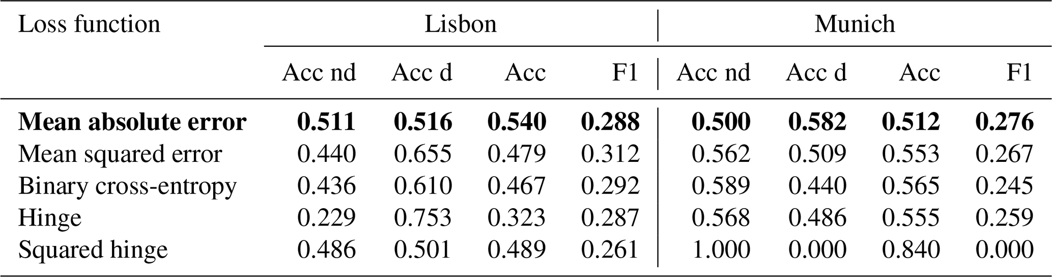
As a next step the influence of the different loss functions on the model performance is investigated. Loss function is a function to evaluate how well a specific algorithm manages to fit the training data (Janocha and Czarnecki, 2016). It is an important part of the optimization function which has a direct influence on the updating of the weights of the ANN (Russell and Norvig, 2009). In addition to overall accuracy and F1 metric, the accuracies of the non-drought and drought classes in the test dataset are displayed. The results are shown in Table 4. Binary cross-entropy, mean absolute error and hinge loss functions show the best performance for the Munich domain. In contrast to that, for the Lisbon domain only the mean absolute error loss function has an accuracy of higher than 0.5. Also in the case of the Munich domain mean absolute error shows a higher performance with regards to the F1 score. Therefore mean absolute error is used for further analysis.
Table 4Performance of the model for different loss functions for the test dataset. Acc nd refers to the accuracy on the non-drought class and Acc d to the accuracy of the drought class. Mean absolute error (bold) is chosen for subsequent analysis since for Munich and Lisbon it shows an accuracy of at least 0.5 for both classes and a higher performance with regards to the F1 score.
3.1.3 Model architecture
Lastly the models are trained on both domains using different architectures. Table 5 displays the model training results for the test dataset. The column “architecture” refers to the number of neurons in each dense (De) layer separated by the *-sign. For dropout (Dr) layers the fraction of weights which are randomly set to zero is given. The model architecture consists overall of seven layers. For example the architecture for the model in the first line of Table 5 is the following:
-
dense layer with 4000 neurons
-
dropout layer randomly setting 50 % of weights to zero
-
dense layer with 1000 neurons
-
dropout layer randomly setting 50 % of weights to zero
-
dense layer with 500 neurons
-
dense layer with 100 neurons
-
dense layer with 5 neurons.
We require the accuracy of both classes individually to be higher than 0.5 and search for an F1 score as high as possible. In the case of the Lisbon domain, three trained models satisfy the criterion of at least 50 % accuracy of each class: the model in the first, in the fourth and in the last row. The best performance in terms of F1 score is obtained for the last model with the following architecture: 5000*0.5*4000*0.5*1000*500*100. For the Munich domain only the first and the fourth models satisfy the criterion of at least 50 % accuracy for each class. For further analyses the first model is chosen as it shows the highest F1 score. The following model architecture is used for the Munich domain: 4000*0.5*1000*0.5*500*100*5. For the best-performing models HSS equals 0.06 for Lisbon and 0.04 for Munich. These results confirm that the obtained prediction is better than the one obtained by a random forecast and therefore does show a weak prediction skill. In the next step those models are analyzed using explainable AI methods.
Table 5Performance of models for the Lisbon and Munich domains for different variations in architecture on the test dataset. Acc nd refers to the accuracy of the non-drought class and Acc d to the accuracy of the drought class. The sixth model architecture is chosen for subsequent analysis for Lisbon and first for Munich (bold) due to an accuracy of at least 0.5 of both classes and a higher performance with regards to the F1 score.

3.2 Explainable AI methods for the analysis of the best-performing algorithms
3.2.1 Shapely values
For the Munich and Lisbon domain Shapely values are calculated using the results of the best-performing models for the test dataset. For the calculation each of the 12 months used as input to the predicting algorithm for each variable is considered individually, resulting in 28 atmospheric variables teleconnection indices variables. The number behind the variable name refers to the number of months before the event (NAO1–NAO value 1 month before the predicted event). The results are shown in Fig. 5. Since the calculation of Shapely values is computationally expensive, they are calculated five times on a subset of 500 data points. The error bars displayed in black on the plot indicate that the uncertainties are smaller than the nominal values of the variable contributions. The nominal Shapely values are normed and recalculated to a percentage of contribution to the prediction; e.g., the NAO1 value explains roughly 2.3 % of the prediction for the Lisbon domain.
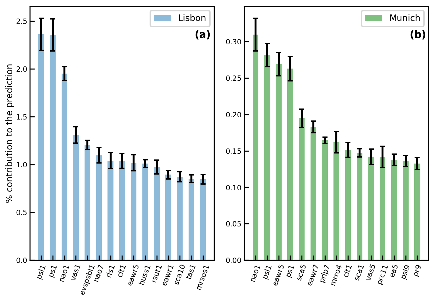
Figure 5Mean Shapely values normalized to the contribution to the prediction for the top 15 variables, with the highest importance for Lisbon (a) and Munich (b) in the test dataset. The number behind the variable name refers to the number of months before the event (NAO1–NAO value 1 month before the predicted event). The results indicate that for the Lisbon domain psl1 and ps1 are the most influential drought predictors; for Munich this is NAO1.
We see that for both domains the contribution to the prediction is broadly distributed among the many input variables. Between Lisbon and Munich, Shapely values show a distinct difference in the nominal values of the feature contributions: values for Lisbon are about 6 times higher than those for Munich (e.g., the contribution of NAO1 for Munich is around 0.3 % and for Lisbon around 1.9 %).
For the Lisbon domain, the variables with a higher-impact are sea level pressure (psl), surface pressure (ps) and NAO 1 month before the event. The first two variables are strongly autocorrelated for the Lisbon domain due to its location at the sea. The strong influence of ps and psl and NAO shows the influence of the atmospheric pressure system on drought formation in Lisbon. It is also striking that the influence of the local pressure seems to be higher than the influence of NAO. The next two variables for the Lisbon domain with the strongest contribution to the prediction are northward near-surface wind (vas) and evaporation (evspsbl). The latter variable has a very direct influence on the formation of drought given that if evaporation is getting lower, the probability of formation of rain clouds also decreases (Sheffield and Wood, 2011). The contribution of vas to drought formation in Lisbon needs to be further studied. For the Munich domain the highest influence is found for NAO1, psl1, EAWR5 and ps1. The results indicate that NAO is the most influential drought predictor for Munich. Additionally the contribution of EAWR5 and SCA5 on the Munich domain cannot be neglected as they are found within the top five predictors. A further investigation of this relationship is of interest for the understanding of drought formation in Munich.
3.2.2 Seasonality
In order to evaluate the influence of seasonality on the prediction the performance of the model is calculated separately for the four seasons. Since the distribution between the drought and non-drought classes is different among the seasons (e.g., range of 17 % to 19 % of drought events for the Lisbon domain) a rescaling of the number of drought and non-drought events is performed to ensure comparability among the results. To compare the performance a precision recall plot is used (Saito and Rehmsmeier, 2015). Recall and precision are calculated for each of the four seasons (MAM, JJA, SON, DJF) and for the 2 half-years (MAMJJA and SONDJF) using the estimated scaling factors. Results of the calculation are shown in Fig. 6. The dotted line marks the line under which the classifier shows no skill. The line is defined as a proportion of drought events against overall number of events (Saito and Rehmsmeier, 2015). For the Lisbon domain it becomes evident that the model performance is very different across seasons: higher precision of around 0.23 can be found during the winter half-year. However for the spring season and summer half-year the recall rises, while precision goes down. For the Munich classifier the results for the different seasons are closer together in terms of recall. It shows a worse performance for the winter months (DJF), while fall, spring and summer show an overall better model performance. This is an indication that for the Munich domain, better drought predictability is possible in spring, fall and summer.
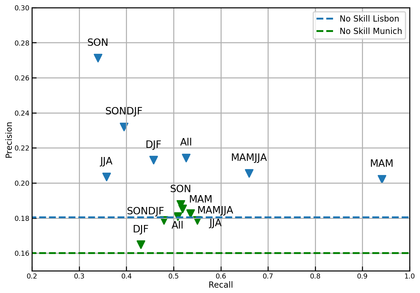
Figure 6The effect of seasonality on precision and recall for Lisbon (blue) and Munich (green). The results indicate that for the Munich and Lisbon domain better drought predictability is possible in spring, fall and summer.

Figure 7Shapely values for Lisbon calculated separately for the four seasons and sorted by the maximum contribution in DJF (a), MAM (b), JJA (c) and SON (d) for the test dataset; evspsbl abbreviated as evp.

Figure 8Shapely values for Munich calculated separately for the four seasons and sorted by the maximum contribution in DJF (a), MAM (b), JJA (c) and SON (d) for the test dataset; sfcWindmax abbreviated as sfcWm.
An additional analysis is conducted to calculate the Shapely values separately for the four season and the two domains in order to understand the influence of the different variables on the prediction. The results of the analysis can be seen in Figs. 7 and 8. The results for the Lisbon domain show that NAO1 is the strongest predictor in winter and spring, while the contribution of pressure to drought predictability is higher in fall, followed by NAO1. In contrast, for the summer season NAO1 is not among the top 10 predictors but rather other teleconnection indices like EAWR5, NAO7 and SCA7. Those teleconnection indices originate from winter months, when NAO was shown to have the highest impact on the prediction. However, given the low performance of the model in the summer season, further investigation is needed. For the Munich domain NAO1 has one of the highest contributions for spring, summer and fall, while it cannot be found among the strongest predictors for winter. EAWR5 is one of the strongest predictors for summer, spring and fall. The feature contributions for predictions in the winter season in Munich indicate that atmospheric variables 10 or 12 months before the event might be drought indicators.
Drought is a multiscale phenomenon, and its formation and evolution are different for every climatology and season. In this study, we (i) explored the possibilities of using the data provided by CRCM5-LE to predict droughts using ANNs and (ii) applied explainable AI methods to gain a better understanding of the results. A drought event is defined as an SPI1 less than −1 at the given site. The first half of the study deals with the systematic search for the best-performing models. For the Lisbon domain the best results are obtained by the model with L2 regularization of 0.001; mean absolute error as a loss function; and the architecture 5000*0.5*4000*0.5*1000*500*100, where five layers are fully connected, and two layers are dropout layers. For the Munich domain, the best results are obtained by the model with L2 regularization of 0.001; mean absolute error as a loss function; and the architecture 4000*0.5*1000*0.5*500*100*5, where five layers are fully connected, and two layers are dropout layers. The best-performing models obtain accuracies of 57 % for the Lisbon domain and 55 % for the Munich domain.
The precision of the prediction in both cases is rather moderate as a high percentage of data are misclassified. For Lisbon, classifier precision remains at around 22 %. This means that one out of four predicted drought events is an actual drought. For the Munich case, this ratio is even lower and amounts to 18 %. However, the models provide an important basis for the development of future drought-predicting models and offer a fruitful ground for the investigation of influence of single input variables during different seasons on drought formation.
Compared to the study by Santos et al. (2014), who investigated drought predictability in Portugal, the weak prediction accuracies of our study are not surprising. In Santos et al. (2014), SPI6 for April, May and June is predicted; however precipitation amounts for the months until March were also given as input. As SPI6 is calculated using the sum of 6 months precipitation, the model receives over half of the information it needs for the calculation of the value. As no similar studies exist for the Munich domain, no comparison can be performed.
The second half of the study concentrates on the analysis of the obtained algorithms using explainable AI methods. Among the strongest predictors for the domains are NAO, psl and ps 1 month before the event. This underlines the importance of the atmospheric system on the drought formation. For the model trained for the Lisbon domain, the variables of northward near-surface wind (vas) and evaporation (evspsbl) followed. For the Munich domain, EAWR and SCA 5 months before the event are found among the strongest predictors. In general the percentages of the contribution of the strongest predictors for the Munich domain are around 6 times lower than those for the Lisbon domain.
This study indicates that seasonality is a crucial factor for drought predictions. Precision and recall of the prediction are lower in summer for the Lisbon domain and in winter for the Munich domain. Moreover, while for the Munich domain the spread of precision and recall across the seasons is rather low, huge differences are found for the Lisbon domain: the trained model obtained higher recall and lower precision for spring and higher precision and lower recall for fall when comparing to the baseline of all data. The results show that for the Lisbon domain, NAO1 is the strongest predictor in winter and spring, while the contribution of pressure to drought predictability is higher in fall, followed by the contribution of NAO1. For the Munich domain, NAO1 is found to have one of the highest contributions for spring, summer and fall, while it could not be found among the 10 strongest predictors for winter.
Further investigations are of interest for scientific research on both objectives. In terms of drought prediction, further research is possible within the same setting. The field of AI is evolving rapidly, showing new algorithms, methods and frameworks, such that there is a high potential for finding better-suited algorithms (Hao, 2019). One of the main limitations of this study remains that an application of the obtained framework on observation data is not possible due to the fact that observational data lack a multitude of variables which are used as input in this study, e.g., heat fluxes and radiation. However the results obtained by Shapely value calculation are of high importance for the choice of variables for the development of a future model which potentially could be applied to observational data. Given the high Shapely importance of NAO for drought prediction, other large-scale variables, such as atmospheric blocking, can be added to the input variables. Moreover, the application to new domains is of interest to investigate the regionality of drought prediction possibilities. Explainable AI methods offer an important approach to improve the current limitations of machine learning models; their application is of high importance in the field of physical geography since it enables a physical interpretation of statistical results to be provided.
Ensemble model data used in this study may be retrieved from the following sources: CanESM2-LE data are available via https://open.canada.ca/data/en/dataset/aa7b6823-fd1e-49ff-a6fb-68076a4a477c (Environment and Climate Change Canada, 2020). CRCM5-LE data can be retrieved at https://climex-data.srv.lrz.de/Public/ (ClimEx project, 2020).
This study was conceptualized by EF under the supervision of RL. Formal analysis, visualization of results and writing of the original draft were performed by EF. All authors contributed to the interpretation of the findings and revision of the paper.
The contact author has declared that neither they nor their co-author has any competing interests.
Publisher's note: Copernicus Publications remains neutral with regard to jurisdictional claims in published maps and institutional affiliations.
This article is part of the special issue “Recent advances in drought and water scarcity monitoring, modeling, and forecasting (EGU2019, session HS4.1.1/NH1.31)”. It is a result of the European Geosciences Union General Assembly 2019, Vienna, Austria, 7–12 April 2019.
The CRCM5-LE was created within the ClimEx project, which was funded by the Bavarian State Ministry for the Environment and Consumer Protection. Computations of the CRCM5-LE were made on the SuperMUC supercomputer at the Leibniz Supercomputing Centre of the Bavarian Academy of Sciences and Humanities. We acknowledge Environment and Climate Change Canada for providing the CanESM2-LE driving data.
This paper was edited by Athanasios Loukas and reviewed by three anonymous referees.
Barnston, A. G. and Livezey, R. E.: Classification, Seasonality and Persistence of Low-Frequency Atmospheric Circulation Patterns, Mon. Weather Rev., 115, 1083–1126, https://doi.org/10.1175/1520-0493(1987)115<1083:CSAPOL>2.0.CO;2, 1987. a
Belayneh, A., Adamowski, J., Khalil, B., and Quilty, J.: Coupling machine learning methods with wavelet transforms and the bootstrap and boosting ensemble approaches for drought prediction, Atmos. Res., 172–173, 37–47, https://doi.org/10.1016/j.atmosres.2015.12.017, 2016. a, b
Biesiada, J. and Duch, W.: Feature Selection for High-Dimensional Data – A Pearson Redundancy Based Filter, in: Computer Recognition Systems 2, edited by: Kurzynski, M., Puchala, E., Wozniak, M., and Zolnierek, A., Springer, Berlin, Heidelberg, 242–249, 2007. a
Bishop, C. M.: Pattern Recognition and Machine Learning (Information Science and Statistics), 1st edn., Springer, Berlin, Heidelberg, 2007. a
Bonaccorso, B., Cancelliere, A., and Rossi, G.: Probabilistic forecasting of drought class transitions in Sicily (Italy) using Standardized Precipitation Index and North Atlantic Oscillation Index, J. Hydrol., 526, 136–150, https://doi.org/10.1016/j.jhydrol.2015.01.070, 2015. a, b, c, d
Bueh, C. and Nakamura, H.: Scandinavian pattern and its climatic impact, Q. J. Roy. Meteor. Soc., 133, 2117–2131, https://doi.org/10.1002/qj.173, 2007. a
Ceglar, A., Zampieri, M., Toreti, A., and Dentener, F.: Observed Northward Migration of Agro-Climate Zones in Europe Will Further Accelerate Under Climate Change, Earths Future, 7, 1088–1101, https://doi.org/10.1029/2019EF001178, 2019. a
Chollet, F., et al.: Keras, available at: https://keras.io (last access: 29 November 2021), 2015. a, b
Clevert, D. A., Unterthiner, T., and Hochreiter, S.: Fast and accurate deep network learning by exponential linear units (ELUs), arXiv [preprint], arXiv:1511.07289, 23 November 2015. a, b
ClimEx project: CRCM5-LE, available at: https://climex-data.srv.lrz.de/Public/ (last access: 30 November 2021), 2020. a
Dawson, A.: eofs: A Library for EOF Analysis of Meteorological, Oceanographic, and Climate Data, Journal of Open Research Software, 4, e14, https://doi.org/10.5334/jors.122, 2016. a, b
Deo, R. C., Kisi, O., and Singh, V. P.: Drought forecasting in eastern Australia using multivariate adaptive regression spline, least square support vector machine and M5Tree model, Atmos. Res., 184, 149–175, https://doi.org/10.1016/j.atmosres.2016.10.004, 2017. a
Enfield, D. B., Mestas-Nuñez, A. M., and Trimble, P. J.: The Atlantic Multidecadal Oscillation and its relation to rainfall and river flows in the continental U.S., Geophys. Res. Lett., 28, 2077–2080, https://doi.org/10.1029/2000GL012745, 2001. a
Environment and Climate Change Canada: The Canadian Earth System Model Large Ensembles, available at: https://open.canada.ca/data/en/dataset/aa7b6823-fd1e-49ff-a6fb-68076a4a477c (last access: 29 November 2021), 2020. a
European Centre for Medium-Range Weather Forecasts: ERA Interim, Daily, available at: https://apps.ecmwf.int/datasets/data/interim-full-daily/levtype=sfc/ (last access: 29 November 2021), 2020.
Federal Ministry of Food and Agriculture: Trockenheit und Dürre 2018 – Überblick über Maßnahmen, available at: https://www.bmel.de/DE/Landwirtschaft/Nachhaltige-Landnutzung/Klimawandel/_Texte/Extremwetterlagen-Zustaendigkeiten.html (last access: 25 July 2019), 2018. a
Folland, C. K., Knight, J., Linderholm, H. W., Fereday, D., Ineson, S., and Hurrell, J. W.: The Summer North Atlantic Oscillation: Past, Present, and Future, J. Climate, 22, 1082–1103, https://doi.org/10.1175/2008JCLI2459.1, 2009. a, b
Goodfellow, I., Bengio, Y., and Courville, A.: Deep Learning, The MIT Press, Cambridge, MA, USA, 2016. a, b
Guyon, I. and Elisseeff, A.: An Introduction to Variable and Feature Selection, J. Mach. Learn. Res., 3, 1157–1182, 2003. a, b
Hao, K.: We analyzed 16,625 papers to figure out where AI is headed next, available at: https://www.technologyreview.com/2019/01/25/1436/we-analyzed-16625-papers-to-figure-out-where-ai-is-headed-next/ (last access: 21 March 2021), 2019. a
Hao, Z., Singh, V. P., and Xia, Y.: Seasonal Drought Prediction: Advances, Challenges, and Future Prospects, Rev. Geophys., 56, 108–141, https://doi.org/10.1002/2016RG000549, 2018. a, b
Hurrell, J. W., Kushnir, Y., Ottersen, G., and Visbeck, M. (Eds.): The North Atlantic Oscillation: Climatic Significance and Environmental Impact, American Geophysical Union, Washington, D.C., 2003. a
IPCC: Climate Change 2013 – The Physical Science Basis: Working Group I Contribution to the Fifth Assessment Report of the IPCC, Assessment report (Intergovernmental Panel on Climate Change), Working Group, Cambridge University Press, Cambridge, England, 2013. a
Janocha, K. and Czarnecki W. M. Wojciech: On Loss Functions for Deep Neural Networks in Classification, Schedae Informaticae, 25, 49–59, https://doi.org/10.4467/20838476SI.16.004.6185, 2016. a
Keyantash, J. and National Center for Atmospheric Research Staff: The Climate Data Guide: Standardized Precipitation Index (SPI), available at: https://climatedataguide.ucar.edu/climate-data/standardized-precipitation-index-spi (last access: 21 March 2021), 2018. a
Kington, J. A.: Daily weather mapping from 1781, Climatic Change, 3, 7–36, https://doi.org/10.1007/bf02423166, 1980. a
Kirchmeier-Young, M., Zwiers, F., and Gillett, N.: Attribution of Extreme Events in Arctic Sea Ice Extent, J. Climate, 30, 553–571, https://doi.org/10.1175/JCLI-D-16-0412.1, 2016. a
Kumar, V. and Minz, S.: Feature selection: a literature review, SmartCR, 4, 211–229, 2014. a
Kushner, P. J., Mudryk, L. R., Merryfield, W., Ambadan, J. T., Berg, A., Bichet, A., Brown, R., Derksen, C., Déry, S. J., Dirkson, A., Flato, G., Fletcher, C. G., Fyfe, J. C., Gillett, N., Haas, C., Howell, S., Laliberté, F., McCusker, K., Sigmond, M., Sospedra-Alfonso, R., Tandon, N. F., Thackeray, C., Tremblay, B., and Zwiers, F. W.: Canadian snow and sea ice: assessment of snow, sea ice, and related climate processes in Canada's Earth system model and climate-prediction system, The Cryosphere, 12, 1137–1156, https://doi.org/10.5194/tc-12-1137-2018, 2018. a
Leduc, M., Mailhot, A., Frigon, A., Martel, J.-L., Ludwig, R., Brietzke, G. B., Giguère, M., Brissette, F., Turcotte, R., Braun, M., and Scinocca, J.: The ClimEx Project: A 50-Member Ensemble of Climate Change Projections at 12-km Resolution over Europe and Northeastern North America with the Canadian Regional Climate Model (CRCM5), J. Appl. Meteorol. Clim., 58, 663–693, https://doi.org/10.1175/JAMC-D-18-0021.1, 2019. a
Lim, Y.-K.: The East Atlantic/West Russia (EA/WR) teleconnection in the North Atlantic: climate impact and relation to Rossby wave propagation, Clim. Dynam., 44, 3211–3222, https://doi.org/10.1007/s00382-014-2381-4, 2015. a
Lundberg, S. and Lee, S.: A unified approach to interpreting model predictions, CoRR, arXiv [preprint], arXiv:1705.07874, 25 November 2017. a
Maas, A. L.: Rectifier Nonlinearities Improve Neural Network Acoustic Models, in: Proceedings of the 30th International Conference on Machine Learning, 16–21 Juni 2013, Atlanta, Georgia, USA, 2013. a, b
Martynov, A., Laprise, R., Sushama, L., Winger, K., Šeparović, L., and Dugas, B.: Reanalysis-driven climate simulation over CORDEX North America domain using the Canadian Regional Climate Model, version 5: model performance evaluation, Clim. Dynam., 41, 2973–3005, https://doi.org/10.1007/s00382-013-1778-9, 2013. a
McGovern, A., Elmore, K. L., Gagne, D. J., Haupt, S. E., Karstens, C. D., Lagerquist, R., Smith, T., and Williams, J. K.: Using Artificial Intelligence to Improve Real-Time Decision-Making for High-Impact Weather, B. Am. Meteorol. Soc., 98, 2073–2090, https://doi.org/10.1175/BAMS-D-16-0123.1, 2017. a, b
McKee, T., Doesken, N., and Kleist, J.: The relationship of drought frequency and duration to time scales, in: Proceedings of the 8th Conference on Applied Climatology, American Meteorological Society Boston, 17–22 January 1993, Anaheim, CA, USA, 1993. a
Mikhailova, N. and Yurovsky, A.: The East Atlantic Oscillation: Mechanism and Impact on the European Climate in Winter, Phys. Oceanogr., 4, 27–36, https://doi.org/10.22449/1573-160X-2016-4-25-33, 2016. a
Morid, S., Smakhtin, V., and Bagherzadeh, K.: Drought forecasting using artificial neural networks and time series of drought indices, Int. J. Climatol., 27, 2103–2111, https://doi.org/10.1002/joc.1498, 2007. a, b
Russell, S. and Norvig, P.: Artificial Intelligence: A Modern Approach, 3rd edn., Prentice Hall Press, Upper Saddle River, NJ, USA, 2009. a, b, c, d, e, f, g, h
Saito, T. and Rehmsmeier, M.: The Precision-Recall Plot Is More Informative than the ROC Plot When Evaluating Binary Classifiers on Imbalanced Datasets, PLoS One, 10, 1–21, https://doi.org/10.1371/journal.pone.0118432, 2015. a, b
Santos, J. F., Portela, M. M., and Pulido-Calvo, I.: Spring drought prediction based on winter NAO and global SST in Portugal, Hydrol. Process., 28, 1009–1024, https://doi.org/10.1002/hyp.9641, 2014. a, b, c
Sasaki, Y.: The truth about of the F-measure, available at: https://www.cs.odu.edu/~mukka/cs795sum09dm/Lecturenotes/Day3/F-measure-YS-26Oct07.pdf (last access: 30 November 2021), 2007. a
Sheffield, J. and Wood, E. F.: Drought: past problems and future scenarios, Earthscan, London, Washington, DC, 2011. a, b, c
Sheffield, J., Andreadis, K. M., Wood, E. F., and Lettenmaier, D. P.: Global and Continental Drought in the Second Half of the Twentieth Century: Severity–Area–Duration Analysis and Temporal Variability of Large-Scale Events, J. Climate, 22, 1962–1981, https://doi.org/10.1175/2008JCLI2722.1, 2009. a, b
Spinoni, J., Naumann, G., Vogt, J., and Barbosa, P.: Meteorological Drought in Europe: Events and Impacts: Past Trends and Future Projections, Publications Office of the European Union, Luxembourg, 2016. a
Spinoni, J., Naumann, G., and Vogt, J. V.: Pan-European seasonal trends and recent changes of drought frequency and severity, Global Planet. Change, 148, 113–130, https://doi.org/10.1016/j.gloplacha.2016.11.013, 2017. a
Trenberth, K.: Changes in Precipitation with Climate Change, Clim. Res., 47, 123–138, https://doi.org/10.3354/cr00953, 2011. a
von Trentini, F., Aalbers, E. E., Fischer, E. M., and Ludwig, R.: Comparing interannual variability in three regional single-model initial-condition large ensembles (SMILEs) over Europe, Earth Syst. Dynam., 11, 1013–1031, https://doi.org/10.5194/esd-11-1013-2020, 2020. a
World Meteorological Organization: Standardized Precipitation Index User Guide, WMO, Geneva, Switzerland, 2012. a
Yoon, J.-H., Mo, K., and Wood, E. F.: Dynamic-model-based seasonal prediction of meteorological drought over the contiguous United States, J. Hydrometeorol., 13, 463–482, 2012. a, b
Zargar, A., Sadiq, R., Naser, B., and Khan, F. I.: A review of drought indices, Environ. Rev., 19, 333–349, https://doi.org/10.1139/a11-013, 2011. a