the Creative Commons Attribution 4.0 License.
the Creative Commons Attribution 4.0 License.
 | 25 Nov 2021
Using high-resolution regional climate models to estimate return levels of daily extreme precipitation over Bavaria
Benjamin Poschlod
Extreme daily rainfall is an important trigger for floods in Bavaria. The dimensioning of water management structures as well as building codes is based on observational rainfall return levels. In this study, three high-resolution regional climate models (RCMs) are employed to produce 10- and 100-year daily rainfall return levels and their performance is evaluated by comparison to observational return levels. The study area is governed by different types of precipitation (stratiform, orographic, convectional) and a complex terrain, with convective precipitation also contributing to daily rainfall levels. The Canadian Regional Climate Model version 5 (CRCM5) at a 12 km spatial resolution and the Weather and Forecasting Research (WRF) model at a 5 km resolution both driven by ERA-Interim reanalysis data use parametrization schemes to simulate convection. WRF at a 1.5 km resolution driven by ERA5 reanalysis data explicitly resolves convectional processes. Applying the generalized extreme value (GEV) distribution, the CRCM5 setup can reproduce the observational 10-year return levels with an areal average bias of +6.6 % and a spatial Spearman rank correlation of ρ=0.72. The higher-resolution 5 km WRF setup is found to improve the performance in terms of bias (+4.7 %) and spatial correlation (ρ=0.82). However, the finer topographic details of the WRF-ERA5 return levels cannot be evaluated with the observation data because their spatial resolution is too low. Hence, this comparison shows no further improvement in the spatial correlation (ρ=0.82) but a small improvement in the bias (2.7 %) compared to the 5 km resolution setup.
Uncertainties due to extreme value theory are explored by employing three further approaches. Applied to the WRF-ERA5 data, the GEV distributions with a fixed shape parameter (bias is +2.5 %; ρ=0.79) and the generalized Pareto (GP) distributions (bias is +2.9 %; ρ=0.81) show almost equivalent results for the 10-year return period, whereas the metastatistical extreme value (MEV) distribution leads to a slight underestimation (bias is −7.8 %; ρ=0.84). For the 100-year return level, however, the MEV distribution (bias is +2.7 %; ρ=0.73) outperforms the GEV distribution (bias is +13.3 %; ρ=0.66), the GEV distribution with fixed shape parameter (bias is +12.9 %; ρ=0.70), and the GP distribution (bias is +11.9 %; ρ=0.63). Hence, for applications where the return period is extrapolated, the MEV framework is recommended.
From these results, it follows that high-resolution regional climate models are suitable for generating spatially homogeneous rainfall return level products. In regions with a sparse rain gauge density or low spatial representativeness of the stations due to complex topography, RCMs can support the observational data. Further, RCMs driven by global climate models with emission scenarios can project climate-change-induced alterations in rainfall return levels at regional to local scales. This can allow adjustment of structural design and, therefore, adaption to future precipitation conditions.
- Article
(16477 KB) - Full-text XML
-
Supplement
(13900 KB) - BibTeX
- EndNote


Extreme rainfall is an important driver for different kinds of hydrometeorological hazards, such as flooding and mass movements. The state of Bavaria is exposed to the highest daily rainfall intensities in Germany. Due to its complex topography and a dense river network, the area is prone to riverine flooding and landslides (Grieser et al., 2006; Wiedenmann et al., 2016). Furthermore, urban areas are at risk of urban flooding due to the dense population and a large fraction of impervious areas (Chen and Leandro, 2019). To assess the risk of heavy precipitation events and to dimension adaptation measures, engineers and public authorities often use the concept of rainfall return levels. In Germany, a rainfall return level database (“Coordinated heavy precipitation regionalization evaluation”, KOSTRA; Junghänel et al., 2017; Malitz and Ertel, 2015) is supplied by the German weather service and is based on rain gauge observations. A similar product is available for Austria (Kainz et al., 2007). MeteoSwiss provides mapped return levels and pointwise data (MeteoSwiss, 2021). These products are included in building standards and are, therefore, widely used. Even though the coverage of rain gauges in Germany, Austria, and Switzerland is relatively high, there are uncertainties due to the spatial representativeness of the measuring stations to generate an area-wide rainfall return level product. This problem applies even more on a continental scale as the rain gauge density is distributed heterogeneously over different European countries, where the available time series might be too short to capture a sufficient number of extreme events (Lewis et al., 2019).
Instead of using pointwise measurements, areal precipitation products (e.g. radar, satellite, or reanalysis products) could be used as the basis for return level calculations. However, each of these areal precipitation products shows different limitations, which lead to uncertain or unrealistic return level estimations. Radar data (RADOLAN for Germany; Kreklow et al., 2020) and satellite products (e.g. CMORPH – Joyce et al., 2004, or PERSIANN – Hong et al., 2004) would provide the necessary temporal and spatial resolutions to capture extreme rainfall events. Yet, the temporal coverage of these products extends only to the early 2000s, which is why the sampling of extreme rainfall events is not sufficient for extreme value analysis. Furthermore, radar estimates (Goudenhoofdt and Delobbe, 2016; Kreklow et al., 2020) as well as satellite products (Stampoulis and Anagnostou, 2012) reveal biases compared to rain gauges. Reanalysis data (e.g. E-OBS – Haylock et al., 2008; ERA-Interim – Dee et al., 2011; ERA5 – Hersbach et al., 2020) would have the necessary temporal coverage, but they show systematic underestimation of the intensity of extreme precipitation events (Hu and Franzke, 2020; own calculations, not shown). Ehmele and Kunz (2019) apply a semi-physical two-dimensional stochastic precipitation model to calculate spatial homogeneous return levels over Baden-Württemberg (Germany). However, the model needs to be calibrated with observational data and therefore relies on the high rain gauge density in the area.
Since the frequency and intensity of heavy precipitation will change due to climate change (Myhre et al., 2019; Poschlod and Ludwig, 2021; Westra et al., 2014), the use of climate models would provide the advantage of being able to estimate climate-change-induced alterations in rainfall return levels on a physical basis. However, this application requires careful validation of climate model results for historical conditions.
Regional climate models (RCMs) at a 12 km spatial resolution have been proven to deliver appropriate rainfall return level estimations for 3-hourly to daily durations (Berg et al., 2019; Poschlod et al., 2021; Nissen and Ulbrich, 2017). Although the results show a high spatial correlation to observational products and a low bias averaged over the area, local deviations are evident, especially in regions with complex topography (Poschlod et al., 2021). Also, the intensity of short-duration hourly rainfall extremes could not be reproduced at a 12 km spatial resolution.
When communicating the results of climate model projections to local or regional stakeholders, insurance companies, and governmental authorities in the fields of flood prevention; hydrological modelling; and dimensioning of reservoirs, buildings, and water infrastructure, these aforementioned local biases may prevent the results from being accepted and implemented (Benjamin and Budescu, 2018). When presenting the study results (Poschlod et al., 2021; Poschlod and Ludwig, 2021) to a selection of representatives of the Bavarian Environment Agency, local deviations in the climate model data stood in the way of further use or even implementation of the study results for adaptation measures to intensifying extreme precipitation events. Such discussion meetings at the interface between climate science and local experts with practical relevance provide valuable insight into practitioner demands. Therefore, one of the objectives of this study is to investigate whether higher-resolution climate models can reduce local biases in extreme precipitation. This could lead to a higher acceptance of extreme precipitation data based on climate models by government institutions, which would also support the implementation of adaptation measures.
For shorter rainfall durations, many studies have shown that higher-resolution RCMs, so-called convection-permitting models (CPMs), improve the reproduction of high-intensity short-duration convectional precipitation events (Brisson et al., 2016; Coppola et al., 2020; Fosser et al., 2014; Kendon et al., 2014). A spatial resolution of a few kilometres is considered necessary by the RCM community to explicitly resolve convection (Langhans et al., 2012; Panosetti et al., 2020; Prein et al., 2015), whereas at broader resolutions parametrization schemes are applied to represent convection. However, long-duration rainfall return levels can also be influenced by convectional precipitation. In Germany, convectional rainfall contributes to the 24-hourly return level for roughly 50 % of the area (Malitz and Ertel, 2015). Therefore, CPMs are expected to improve the estimations of these return levels as well. Additionally, the higher spatial resolution enhances the representation of complex terrain (Karki et al., 2017; Langhans et al., 2012; Poschlod et al., 2018).
Hence, in this study, three different high-resolution RCMs featuring 12, 5, and 1.5 km spatial resolutions and driven by 30-year reanalysis data are applied to reproduce daily 10- and 100-year rainfall return levels over the complex terrain of the northern Prealps and Alps. Based on interviews with stakeholders from the infrastructure sector and on legislative guidelines, Nissen and Ulbrich (2017) identified the 10-year return level as a relevant threshold. Following this recommendation, the 10-year return level is chosen in this study as well, representing “moderate extremes”. However, since the insurance industry (Ehmele and Kunz, 2019) and flood protection specialists (Schmitt and Scheid, 2020) are interested in longer return periods, 100-year return levels are calculated despite the higher extreme value statistical uncertainties. The daily duration is relevant for the generation of riverine floods in the study area (Berghuijs et al., 2019; Keller et al., 2017; Merz and Blöschl, 2003), such as the two extreme flooding events in May 1999 and August 2005 in southern Bavaria, Austria, and Switzerland (BLFW, 2003; Grieser et al., 2006; LfU, 2007; Stucki et al., 2020) induced by high daily precipitation sums. However, the antecedent wetness state of the catchment also plays a major role in the transition of heavy precipitation to floods (Schröter et al., 2015).
The daily 10- and 100-year return levels based on the three RCM setups are evaluated by means of an observational return level product using national datasets from Germany, Austria, and Switzerland. In a second step, different extreme value distributions and sampling strategies are applied to all climate model datasets to explore uncertainties due to extreme value theory and to investigate possible improvements.
The study tries to answer two main research questions: (1) can existing RCM setups at higher spatial resolutions reduce local biases and improve spatial correlation between the climate model products and the observational product? (2) How large are the differences due to the application of different state-of-the-art extreme value statistical approaches and which approach is recommended?
2.1 Observational rainfall return level data
To evaluate the RCMs, an observation-based product is generated from the three national datasets described below. As these datasets extend to the national borders and a little beyond, the arithmetic mean is calculated in the overlapping areas. To compare gridded precipitation from the RCMs and point measurements from the observations, Breinl et al. (2020) suggest an areal reduction of 5 % for pointwise 24-hourly 10-year return levels in Austria. However, to be consistent over the study area, no areal reduction factor is applied to the daily duration following Berg et al. (2019) and Poschlod et al. (2021).
2.1.1 Germany
The German weather service offers gridded return level data derived from daily rain gauge measurements (Malitz and Ertel, 2015). The daily measurement window spans 05:50 to 05:50 UTC the next day. The observations cover a maximum period of 1951–2010, where only May–September are analysed as the highest rainfall amounts occur during these months. A peak over threshold (POT) sampling strategy was applied to 2231 rain gauges, where the threshold corresponds to the available time period. A maximum of 2.718 events per year on average was considered. For these samples, an exponential distribution was fitted. The resulting daily return levels are increased by 14 % to provide 24-hourly moving-window estimates (Malitz and Ertel, 2015). The rainfall return levels were spatially interpolated over Germany at a roughly 8×8 km2 resolution. An uncertainty range of 15 % (20 %) is assumed for the 10-year (100-year) return levels, which is induced by measurement errors, uncertainties in the extreme value statistics and regionalization, and the internal variability in the climate system (Junghänel et al., 2017). Data are accessed from DWD (2020). As the daily return levels were transferred to 24-hourly moving-window estimates beforehand, I reduce these values by 14 % to obtain daily estimates. This relation between daily fixed windows and 24-hourly moving windows has also been applied by Poschlod et al. (2021) following Barbero et al. (2019) and Boughton and Jakob (2008).
2.1.2 Austria
The Austrian dataset follows a similar approach to the German dataset, also applying POT sampling at 141 ombrographs (5 min resolution) and 843 ombrometers (daily resolution 06:00 to 06:00 UTC the next day) spatially interpolated to gridded return levels at a 6×6 km2 resolution (BMLRT, 2018). As the rain gauges are distributed inhomogeneously, yielding return level estimations that are too low, the “orographic convective model” OKM (Lorenz and Skoda, 2001) was employed to support the observations (Kainz et al., 2007). The resulting design rainfall is based on a combination of the observational data and the weather model simulations. Further details can be found in Kainz et al. (2007) and BMLRT (2006, 2018). Data are accessed from BMLRT (2020). Again, this data product provides moving-window 24-hourly estimates, which is why the 24-hourly return levels are adjusted to daily values applying a reduction of 14 % (see Sect. 2.1.1).
2.1.3 Switzerland
MeteoSwiss (2021) provides pointwise daily rainfall return levels at 336 rain gauges. The daily measurement extends from 05:40 to 05:40 UTC the next day. The observations cover the time period from 1966 to 2015. To increase the sample size, seasonal maxima were extracted and assumed to follow a generalized extreme value (GEV) distribution. The GEV distribution is fitted via Bayesian estimation, and the according return levels are generated (Fukutome et al., 2015). Since an areal comparison product is to be produced in this study, these point return levels are regionalized by means of ordinary kriging.
2.2 Climate model data
Three different RCM setups are used: the Canadian Regional Climate Model version 5 (CRCM5) driven by ERA-Interim, the Weather and Research Forecasting (WRF) model (Skamarock et al., 2008) driven by ERA-Interim, and WRF driven by ERA5. The selection of these three different setups was based on the following considerations: CRCM5 driven by a global climate model ensemble has been proven to reproduce rainfall return levels over Europe with good skill (Poschlod et al., 2021). However, the study has shown that internal climate variability has major impacts on the estimation of return levels. Using reanalysis data as boundary conditions strongly reduces this source of uncertainty when comparing with observation-based return levels. As described in Sect. 1, the resulting return levels of this RCM driven by a global climate model ensemble were presented to local authorities, but local biases prevented further implementation of the results. Therefore, the CRCM5 setup serves as a benchmark. WRF ERA-Interim at a 5 km resolution represents a setup optimized for the study area with a higher spatial resolution but parametrization of convection. WRF ERA5 is the highest-resolution setup available with a 1.5 km resolution and calculates convection explicitly. All three climate model rainfall datasets are openly available.
2.2.1 CRCM5 ERA-Interim
CRCM5 at a 0.11∘ resolution equalling roughly 12 km is driven by ERA-Interim reanalysis data (Leduc et al., 2019). No nesting was applied, as with the RCM setups presented in Kotlarski et al. (2014), which are also driven by ERA-Interim and have a spatial resolution of 0.11∘. Convectional processes are parametrized due to the spatial resolution. Processes related to deep convection are calculated with the parametrization scheme by Kain and Fritsch (1990). The Kuo transient scheme (Bélair et al., 2005; Kuo, 1965) is applied to represent shallow convection. A more detailed documentation of the model setup and options used is given by Hernández-Díaz et al. (2012) and Martynov et al. (2012). Daily rainfall sums of the 30-year time period of 1980–2009 are extracted for this study.
2.2.2 WRF ERA-Interim
WRF version 3.6.1 is set up in nested domains of 45×45, 15×15, and 5×5 km2 spatial resolution in its non-hydrostatic mode and driven by ERA-Interim (ERA-I) reanalysis data at 75×75 km2 spatial resolution and 6-hourly temporal resolution (Warscher et al., 2019). Spectral nudging is applied to reduce deviations from the large-scale forcing patterns in the reanalysis data (Wagner et al., 2018). Convection is parametrized with the Grell–Freitas scheme (Grell and Freitas, 2014). The detailed model setup as well as an evaluation of different climate variables is given in Warscher et al. (2019). Here, daily rainfall data of the highest-resolution domain are used for the time period of 1980–2009. Data are accessed from Warscher (2019).
2.2.3 WRF ERA5
The WRF model version 4.1 is configured with two one-way nested domains of 7.5×7.5 and 1.5×1.5 km2 grid spacing centred over Bavaria (Collier and Mölg, 2020). The model is forced at the outer lateral boundaries by ERA5 reanalysis data at a 30×30 km2 spatial resolution and 3-hourly temporal resolution applying spectral nudging. The higher-resolution 1.5 km setup is assumed to explicitly resolve convection, and therefore no parametrization scheme is applied. The 30-year simulation was divided into 30 annual slices starting at 1 September of each year. As the model is forced by the lateral boundary conditions at a 3-hourly resolution, slicing the simulation period is not assumed to have a systematic impact on the magnitude of rainfall return levels. A detailed description of the model setup and evaluation of various climate variables are provided in Collier and Mölg (2020). However, the authors emphasize that the applied schemes and the model configuration have not been optimized for the study area due to the high computational expenses of the high-resolution run. The physics and dynamics options used in the simulations are based on former convection-permitting WRF applications (e.g. Collier et al., 2019). In this study, daily rainfall sums from 1988–2017 are extracted from the climate model data accessed from Collier (2020). The 1.5 km domain covers 351×351 grid cells, whereby the outer 40 cells are discarded on all sides to exclude boundary effects (Collier and Mölg, 2020).
2.3 Description of the study area
The area of investigation is given by the analysis domain of the highest-resolution RCM, which is centred over the state of Bavaria, and the available observational rainfall return level data (see Fig. 1). It covers south-eastern Germany, north-western Austria, north-eastern Switzerland, and Liechtenstein. The area shows altitude levels below 100 m in the north-west in the Rhine plain up to altitudes above 2500 m in the Alps. It covers various low mountain ranges, including the Ore Mountains, Odenwald, Swabian Jura, and Bavarian Forest. The patterns of annual mean precipitation are governed by the complex topography (see Fig. 2; Haylock et al., 2008). Different rainfall types (convectional, orographic, stratiform) contribute to this precipitation climatology (Malitz and Ertel, 2015). The lowest annual precipitation sums amount to 500–700 mm in the north of the study area. The low mountain ranges induce orographic lifting, leading to precipitation sums of 1000 to 1500 mm yr−1. The highest precipitation sums of more than 2000 mm are found in the Alps, with dry valleys, such as the Inn valley, having totals below 1000 mm. Annual average temperatures range from less than 0 ∘C in the Alps to 10 ∘C in northern Bavaria (DWD, 2021; ZAMG, 2021).
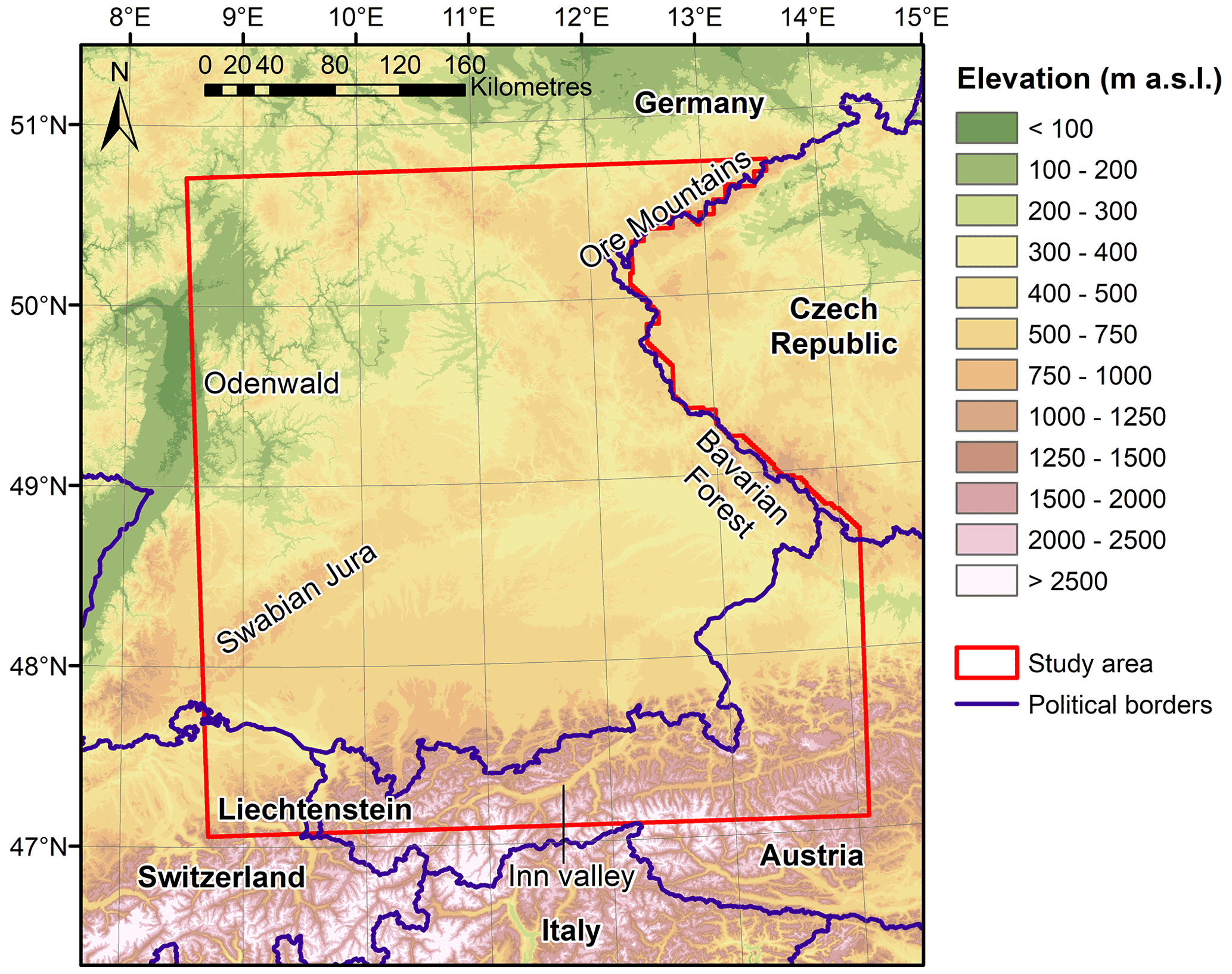
Figure 1Topography of the investigated area. The elevation is based on the Shuttle Radar Topography Mission (SRTM) at a 90 m resolution (Jarvis et al., 2021).
Extreme value theory (EVT) is applied to quantify the stochastic behaviour of a process at unusually large or small values. It is commonly used to calculate return levels for different rainfall durations (Coles, 2001).
3.1 Block maxima
A classical approach to sample unusual (“extreme”) rainfall intensities is given by the block maxima (BM) approach (Coles, 2001). Therein, a single value is extracted from a typically seasonal or annual block. This strategy ensures that the samples are distant from each other, leading to very low serial dependence. However, not all sampled values might be extreme. Also, the information of more than one extreme value per block is lost as these values are discarded.

Figure 2Annual mean precipitation for the period 1980–2009 based on E-OBS (Haylock et al., 2008).
The Fisher–Tippett–Gnedenko theorem (Fisher and Tippett, 1928; Gnedenko, 1943) states that the distribution of the block maxima samples tends to follow the GEV distribution, where the cumulative density function (CDF) G is given with the sample size n→∞:
The location parameter μ governs the centre, and the scale parameter σ governs the spread of the GEV distribution. The tail behaviour of G is defined by the shape parameter ξ, determining whether the GEV follows the Weibull (ξ<0), Gumbel (ξ=0), or Fréchet (ξ>0) distribution (Gilleland et al., 2017). Hence, the GEV is a very flexible distribution. The drawback of this flexibility shows up in a high estimation variance of ξ resulting in an unstable quantile estimate (Bücher et al., 2021).
For all three RCM setups, annual maxima of daily precipitation are extracted. Then for all grid cells trends are detected applying the Mann–Kendall test at the significance level of α=0.05. The significance level describes the probability of rejecting the null hypothesis H0 given that H0 is true. As the statistical test is carried out at n grid cells, H0 would be erroneously rejected at n⋅α grid cells on average by design of the test setup (Ventura et al., 2004). The rate of these errors is referred to as the false discovery rate (FDR; Benjamini and Hochberg, 1995). To control the FDR, the critical p value is adjusted for multiple testing using the approach from Benjamini and Hochberg (1995) following Wilks (2016). H0 is rejected at each grid cell g if the p value of the test pg≤pFDR, where
p(g) with g=1, …, n comprises the sorted p values of the statistical test for all grid cells g of the study area. For αFDR the value of 2⋅α is recommended (Wilks, 2016).
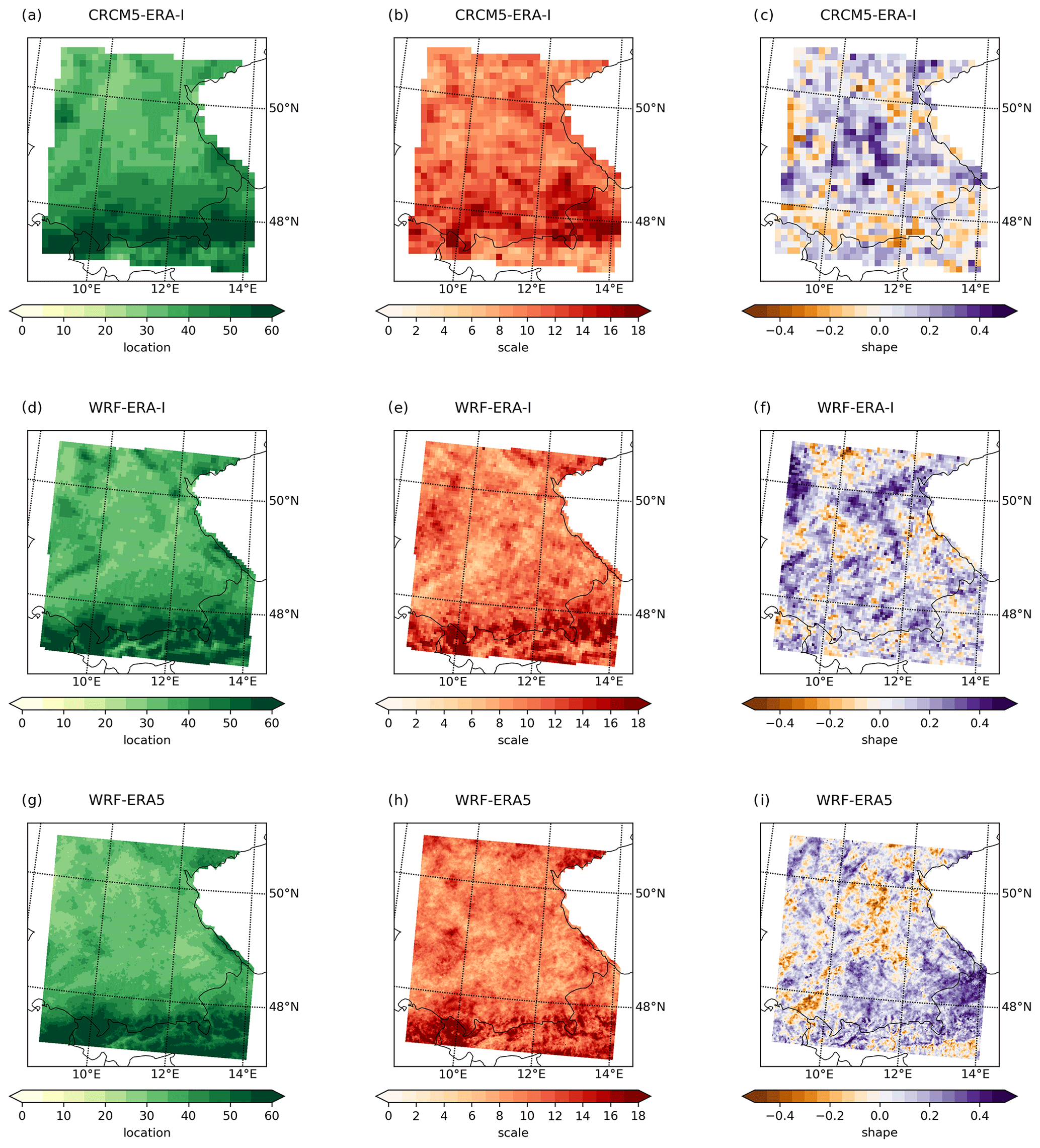
Figure 3Location, scale, and shape parameters of the GEV-LMOM approach based on CRCM5 ERA-Interim (a–c), WRF ERA-Interim (d–f), and WRF ERA5 (g–i).
No significant trends are found for the 30 sampled values at each grid cell of every RCM setup. The parameters of the GEV distribution G are optimized to the BM samples by estimating the L-moments (Hosking et al., 1985). This is carried out applying the R package “extRemes” by Gilleland and Katz (2016). Delicado and Goria (2008) recommend the method of L-moments for sample sizes of n≤50 as it is robust to outliers in the data. The Anderson–Darling test at the significance level of α=0.05 is applied to ensure the goodness of fit of the estimated GEV distribution at each grid cell (see Fig. S7). Again, the critical p value is adjusted for multiple testing. Less than 0.15 % of all fits for all three climate model setups are rejected. Based on these fits, the 10- and 100-year return levels are derived. The spatial distributions of the GEV parameters are mapped in Fig. 3.
There, the location parameter is governed by the topography (see Figs. 1 and 3a, d, g), where the spatial distribution of these parameters is similar for all three RCM setups. The spatial distribution of the scale parameter also corresponds to the topography but shows more noise. The spatial distributions of WRF ERA-I and WRF ERA5 are similar and show the highest values of the scale parameter at the northern slopes of the Alps. The orography of the low mountain ranges of the Swabian Jura, Odenwald, Ore Mountains, and Bavarian Forest also impacts the spatial pattern of the scale parameter (Fig. 3e and h). Lower values are found at the lee sides of the low mountain ranges and the inner Alpine dry valleys. The spatial distribution of the scale parameter based on CRCM5 ERA-I follows the topography less closely and shows an even noisier pattern (Fig. 3b). Some topographical features can nevertheless be recognized, such as the Odenwald and higher values in the Prealps and on the northern slopes of the Alps. The fitted shape parameter reveals a chaotic pattern with small patches of positive and negative values differing for the three RCM setups. This chaotic pattern corresponds to the high estimation variance of the shape parameter based on the limited available sample size of 30 annual maxima.
The histograms of the parameters are given in the Supplement (Fig. S1 in the Supplement). An exemplary fit for the grid cell of Munich is shown in Fig. S2 for all three RCM setups. This EVT approach is referred to as GEV-LMOM.
As small samples lead to high uncertainties in estimating the shape parameter of the GEV distribution, Papalexiou and Koutsoyiannis (2013) recommend using a fixed value of ξ=0.114. This approach is referred to as GEV-FIX. The Anderson–Darling test at the significance level of α=0.05 is carried out in the same way as for GEV-LMOM (see Fig. S7). Fewer than 0.01 % of all fits are rejected. Figure S3 provides an exemplary fit for the grid cell of Munich.
3.2 Peak over threshold
The second classical approach of peak over threshold (POT) tries to overcome the drawbacks of the BM sampling as all values s above a threshold u are sampled as extreme values (Balkema and de Haan, 1974; Pickands, 1975). Therefore, multiple values per block are allowed. However, additional restrictions have to be introduced to ensure approximately independent samples. To prevent successive data points from being sampled that originate from one persistent rainfall event, the time series has to be de-clustered. Therefore, a temporal threshold tdecluster is chosen and all values within the duration of tdecluster around the sampled extreme value are discarded (Coles, 2001).
For the POT approach, the exceedances are sampled for the threshold u and samples s>u. Thereby, the number of exceedances per year is assumed to follow a Poisson distribution (Davison and Smith, 1990). The exceedances y of the POT threshold u are described by the two-parameter generalized Pareto (GP) distribution (Davison and Smith, 1990; Martins and Stedinger, 2001). The corresponding CDF is given by
where y defines the precipitation excess over the threshold u of the POT sampling. The scale parameter β and shape parameter ξ describe the spread and tail behaviour of the GP distribution (Coles, 2001).
The GEV and the GP frameworks can be expressed by the other one as the GP distribution corresponds to the tail distribution of the GEV (Coles, 2001; Goda, 2011; Serinaldi and Kilsby, 2014).
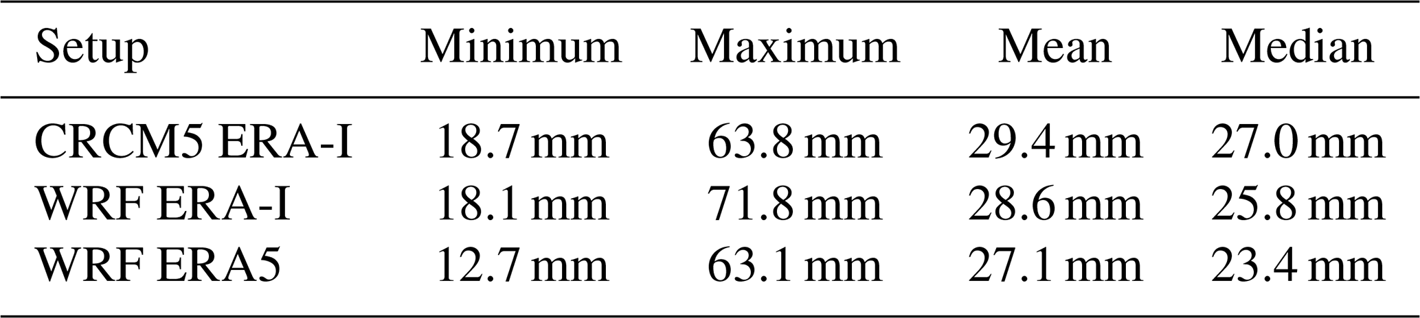
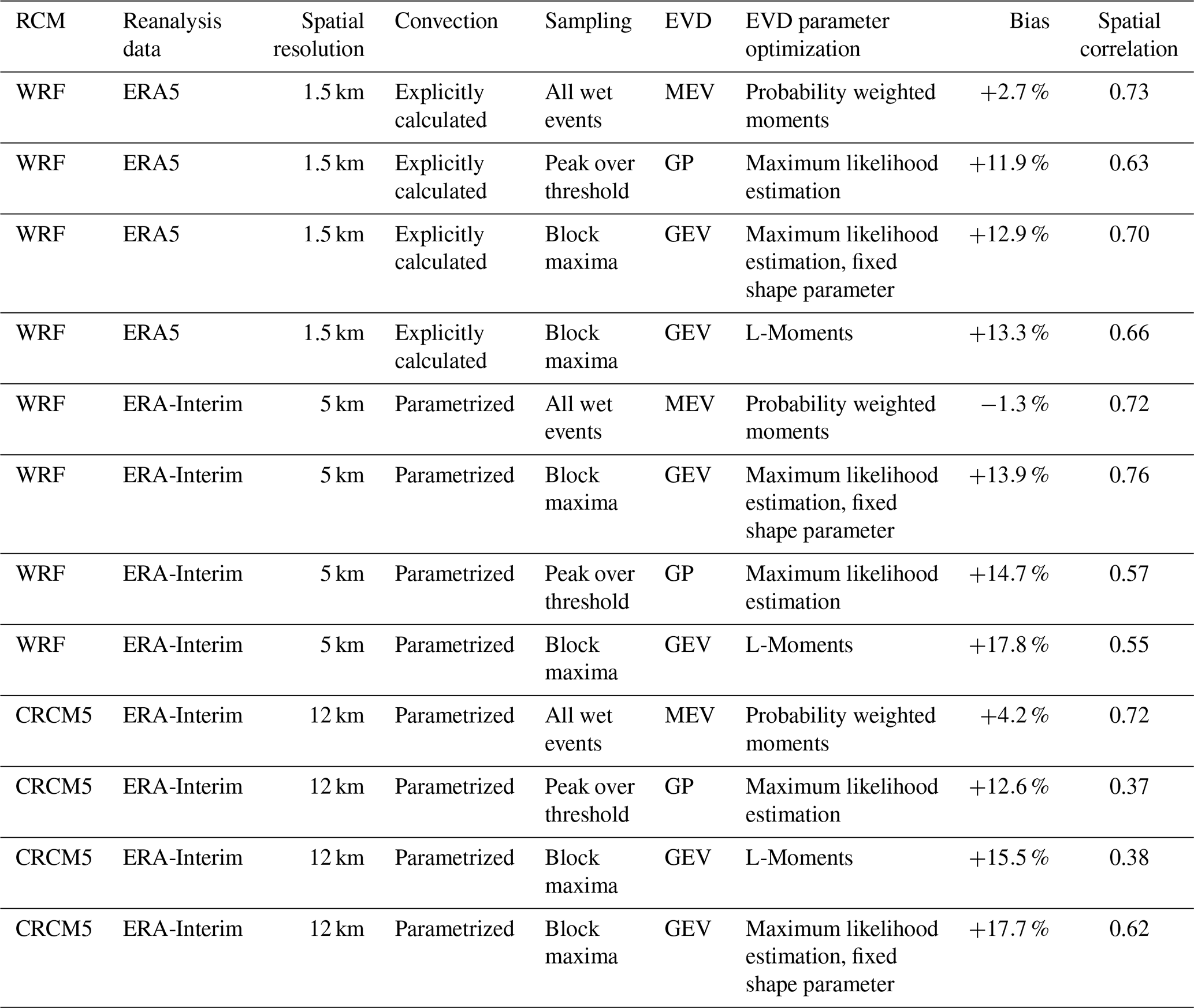
For the POT approach, the daily rainfall time series is de-clustered applying a conservative threshold tdecluster of 5 d. Typical continental cyclones are found to last up to 2.25 d in Bavaria, whereas van Bebber-type Vb cyclones can last up to 3 d (Hofstätter et al., 2018; Mittermeier et al., 2019). Hence, the threshold of 5 d ensures approximately independent samples. Precipitation intensities are assumed to be extreme when exceeding the threshold given by 90 events per 30-year period. This threshold has also been selected by Berg et al. (2019). Statistical properties of the thresholds are given in Table 1 for all three RCM setups. Trends are excluded in the same way as for the GEV-LMOM approach. For sample sizes of n>50, Delicado and Goria (2008) and Madsen et al. (1997) recommend maximum likelihood estimation (MLE) as an optimization algorithm to fit an extreme value distribution. Following this recommendation, MLE is applied to fit the GP distribution to the 90 samples per grid cell using the software package by Gilleland and Katz (2016). The goodness of fit is assessed in the same way as for the GEV-LMOM approach (see Fig. S7), leading to a rejection of 0.15 % of all fits. An exemplary fit for the grid cell of Munich is shown in Fig. S4. This approach is referred to as GP-MLE.
Table 1Statistical properties of the POT threshold u for the three different model setups in the study area.
3.3 Metastatistical extreme value framework
For both classical approaches only a limited number of samples contribute to the database of extreme values. A newer approach by Marani and Ignaccolo (2015) samples all “wet” events assuming that the information of these “ordinary” values can be used to estimate the distribution of extreme values. Thereby, wet events are defined by a threshold twet. It has been successfully applied to extreme daily precipitation by Zorzetto et al. (2016).
The approach by Marani and Ignaccolo (2015) features the metastatistical extreme value (MEV) distribution. They propose a framework supposing that the “metastatistic” of the rainfall sums of wet events per year contains information about the intensity of extreme events. They assume the sampled wet days > twet to be independent following that the probability distribution of maxima ζm can be expressed as , where nj is the number of wet events in a year and F(x) is a distribution describing the rainfall sums of these events. Based on the results of Wilson and Toumi (2005), the distribution of rainfall sums during wet days per year is found to follow a distribution with an exponential tail. They expressed precipitation as the product of mass flux, specific humidity, and precipitation efficiency. Following statistical relationships, they concluded that the tail of the distribution of the product of these three random variables is given by a stretched exponential form. Marani and Ignaccolo (2015) and Zorzetto et al. (2016) apply a Weibull distribution to describe this relationship. Hence, Weibull parameters have to be estimated for each year based on all wet events of a year. The MEV-Weibull CDF is given by
where j is the year (j=1, 2, …, M) and nj is the number of wet events in year j. Cj and wj describe the scale and shape of the Weibull distribution (Marani and Ignaccolo, 2015).
Wet days are defined by exceedance of the threshold twet=1 mm d−1 in accordance with WMO guidelines (Klein Tank et al., 2009). This also accounts for the behaviour of RCMs to produce too many very low intensity precipitation days (“drizzle effect”; Gutowski et al., 2003). As the MEV framework requires the ordinary wet events to be independent (Miniussi et al., 2020) and temporal autocorrelation of rainfall over mountainous areas tends to be higher (Marra et al., 2021), the autocorrelation of daily rainfall is analysed following Marra et al. (2018; see Fig. S5). In the study area, multi-day precipitation events are common especially at the mountain slopes (Kunz and Kottmeier, 2006; Pöschmann et al., 2021). Therefore, the temporal autocorrelation is calculated for lag times of up to 30 d. The autocorrelation between 10 and 30 d drops to very low values and can be assumed to represent noise without any statistical or meteorological correlation (Marra et al., 2018). The 75th quantile of this long-lag noise is chosen as the “noise threshold”. The minimum distance allowed between ordinary events equals the time lag when the autocorrelation first drops below the noise threshold. Hence, the minimum time interval between ordinary wet events may vary within the grid cells, but the independence of the events is ensured by this methodology. The Weibull distribution is fitted to the annual wet events by means of the probability weighted moment (PWM) method (Greenwood et al., 1979) following Zorzetto et al. (2016). Here, the MLE is not used as an estimation method, as the number of wet events per year amounts to 40 events on average due to the de-clustering to remove the temporal autocorrelation. For small sample sizes, the MLE estimator for Weibull parameters is known to be biased (Ross, 1996), whereas the PWM method delivers unbiased estimations (Heo et al., 2001). The MEV fitting procedure and the calculation of return levels are carried out using the Python software package “mevpy” (Zorzetto, 2021). The goodness of fit of the annual wet events applying the Weibull distribution is tested with a Kolmogorov–Smirnov test at the significance level of α=0.05, where the p value is adjusted for multiple testing. Fewer than 0.06 % of all 30 annual fits per grid cell are rejected for all climate models. This approach is referred to as MEV-PWM. An exemplary comparison of the resulting return level curve to the empirical annual maxima is shown in Fig. S6 for the grid cell of Munich.
4.1 Evaluation of 10-year return levels
All approaches and their performance metrics are summarized in Table 2. A mapped comparison of the 10-year return levels calculated via GEV-LMOM based on the three different RCM setups is given in Fig. 4. For a better visualization, the observational product is bilinearly interpolated to the respective RCM grid. The following metrics are calculated for the original data (see Fig. S14 for the natively resolved observational product). The observational product shows the highest rainfall intensities above 100 mm d−1 at the northern slopes of the Alps. The low mountain ranges of the Bavarian Forest, Swabian Jura, Odenwald, and Ore Mountains also induce enhanced intensities of between 70 and 100 mm d−1. The lowest return levels are observed in the north of the study area, amounting to intensities below 50 mm d−1 (Fig. 4b, e, and h). The 12 km resolution CRCM5 ERA-I can reproduce the general spatial pattern with a Spearman rank correlation of ρ=0.72 (Fig. 4a). The return levels are generally overestimated north of 48∘ N and underestimated south of 48∘ N as well as in the Ore Mountains (Fig. 4c). The spatially averaged bias amounts to +6.6 %. The range of simulated rainfall return level intensities is similar to the observations for the whole study area (Fig. 5a) as well as for the southern Alpine part (Fig. 5d). However, the histogram also reveals that the bias stems from simulating too few grid cells with return level intensities of between 50 to 60 mm d−1 and too many grid cells with return levels at intensities of 70 to 90 mm d−1 (Fig. 5a).
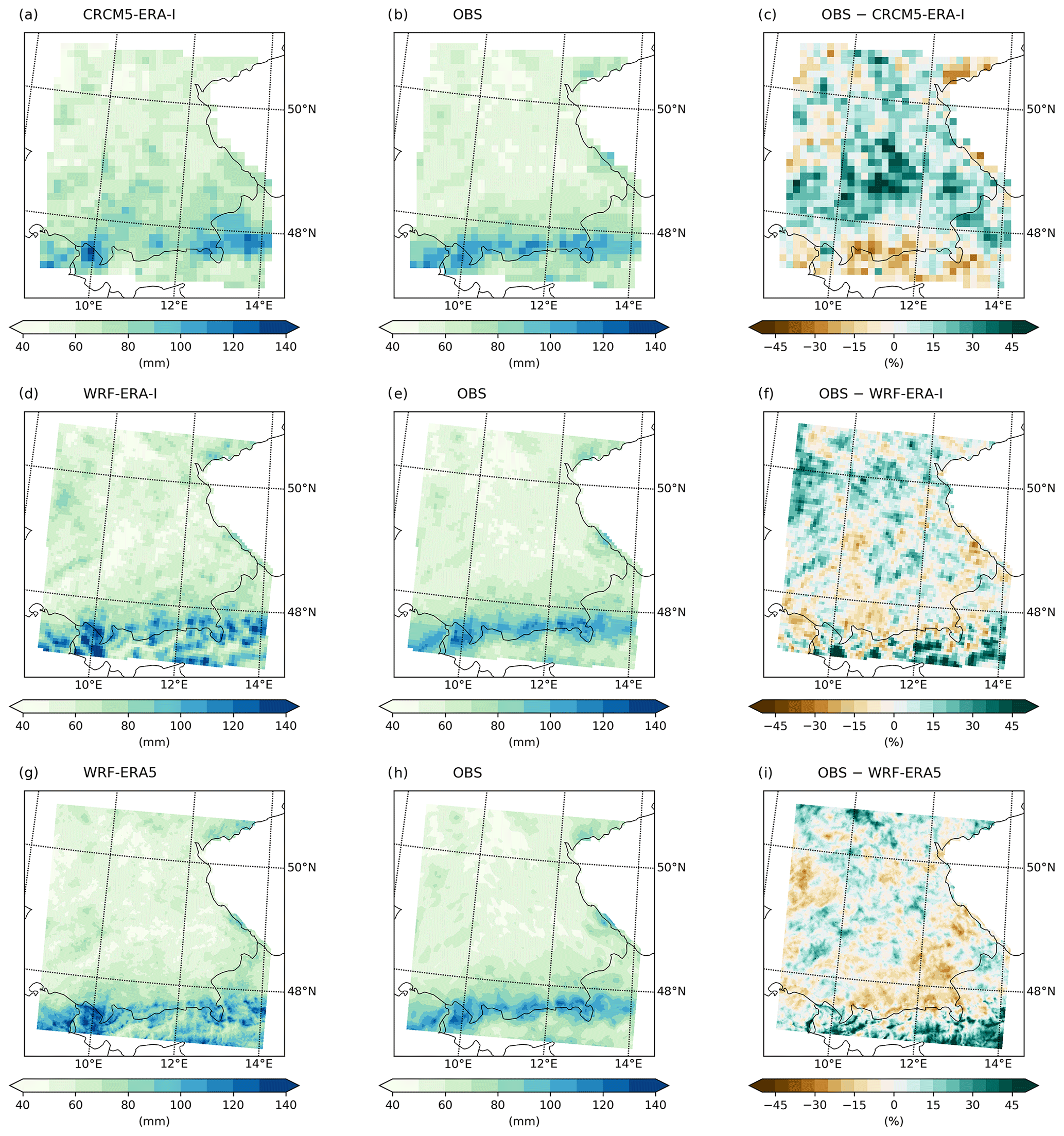
Figure 4The 10-year rainfall return levels applying GEV-LMOM based on CRCM5 ERA-Interim (a), WRF ERA-Interim (d), and WRF ERA5 (g). The middle column (b, e, h) shows the observational product bilinearly interpolated to the respective climate model grid. The right column (c, f, i) provides the percentage difference calculated as the climate model return level minus the observational return level.
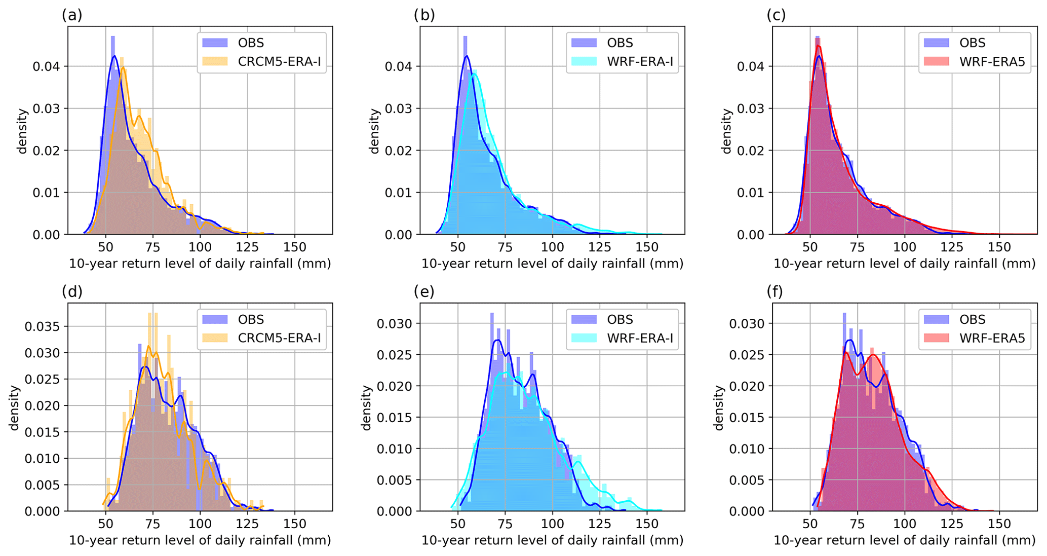
Figure 5Histograms of the resulting 10-year return levels in the whole study area (a–c) and the Alpine area south of 48∘ N (d–f). Gaussian kernel density estimates are plotted to enhance the readability.
Table 2Summary of the applied RCM setups and EVT approaches. Performance metrics of the comparison to observational 10-year return levels are given in terms of the spatially averaged bias and spatial correlation (Spearman). The entries are sorted first by resolution and then by amount of bias.
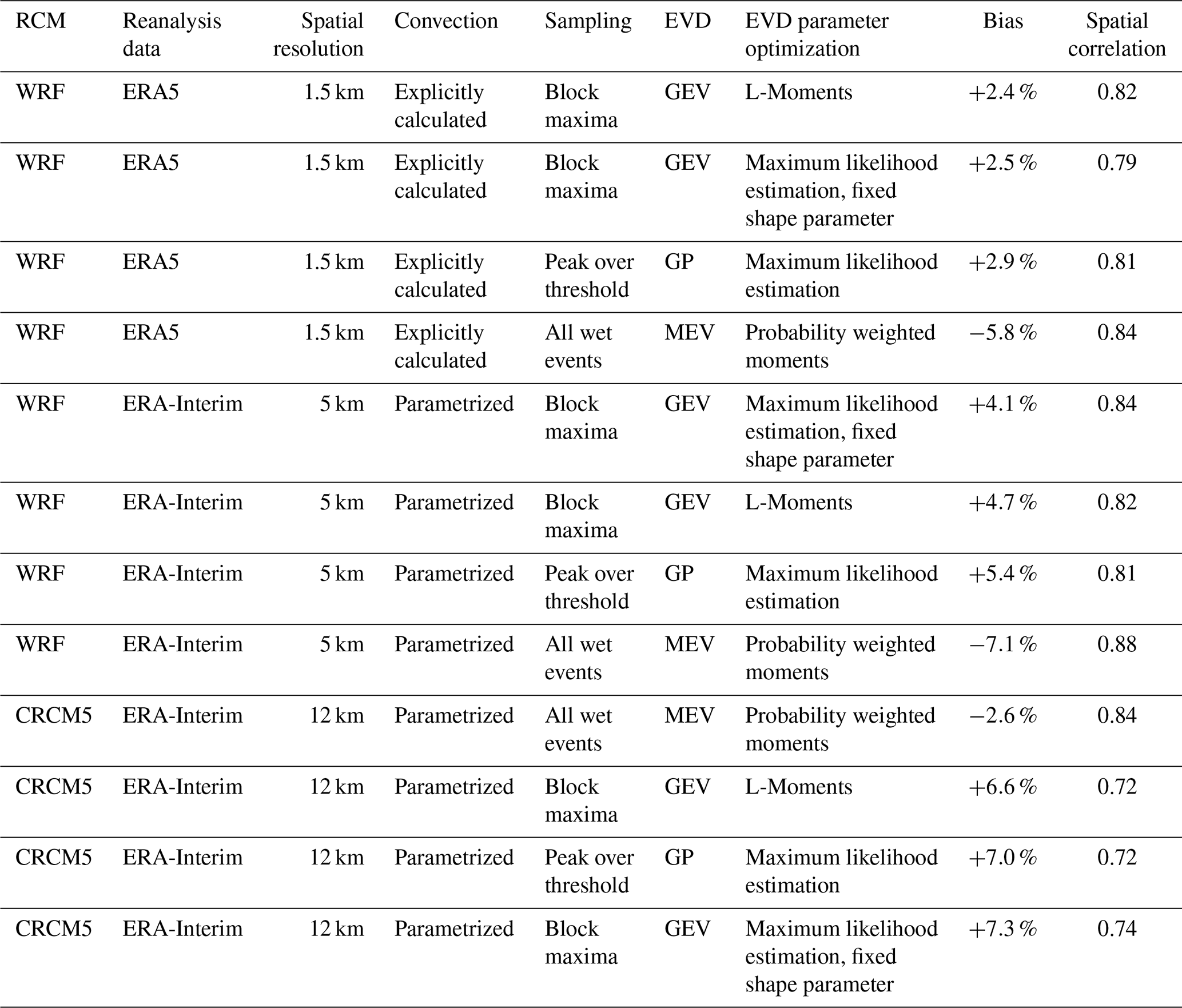
The 10-year return levels based on WRF ERA-I at a 5 km resolution can recreate the spatial pattern of the observations with a Spearman correlation of ρ=0.82 (Fig. 4d). The higher intensities due to the orographic precipitation at the lower mountain ranges and their spatial patterns are reproduced, though the intensity around the Bavarian Forest is underestimated. In the Alpine area, WRF ERA-I simulates higher intensities than observed, especially in the Alps south-east of the Inn valley. However, the results also show a very pronounced orographic signal with low return levels in the major Alpine valleys, which has also been described by Warscher et al. (2019). The overall bias amounts to +4.7 %. The histogram of simulated return levels is similar to the observed histogram (Fig. 5b); however, the very high intensities above 110 mm d−1 in the Alpine area are overrepresented. Also, the range of simulated return levels extends to over 140 mm d−1 (Fig. 5e).
The 10-year return levels based on WRF ERA5 show a generally similar spatial pattern to those of WRF ERA-I (Fig. 4g and d). The spatial pattern of orographic precipitation around the low mountain ranges is recreated, whereby the intensities at the Bavarian Forest and the Odenwald are underestimated. The return levels in south-eastern Bavaria are underestimated as well. As with WRF ERA-I, WRF ERA5 also simulates high return levels above 100 mm d−1 in the Alps south-east of the Inn valley. This results in a Spearman correlation of ρ=0.82. The spatial average of the bias amounts to +2.4 %. The range and distribution of the simulated return levels are very close to the observations for the whole study area (Fig. 5c) as well as south of 48∘ N (Fig. 5f).
Figure 6 compares the three different EVT approaches of GEV-FIX, GP-MLE, and MEV-PWM based on WRF ERA5. The intensities as well as the resulting spatial distribution of GEV-FIX and GP-MLE are very similar to those of GEV-LMOM (Figs. 4g, 6a and d). The spatial correlation between GEV-FIX and the observations amounts to ρ=0.79 and the overall bias to +2.5 %. For GP-MLE, the spatial correlation is ρ=0.81 and the overall bias is +2.9 %. The MEV-PWM method also shows a similar spatial pattern (Fig. 6g), which is slightly more homogeneous than those of GEV-LMOM or GP-MLE. The 10-year return levels based on MEV-PWM are estimated to be generally lower than those of the classical approaches. The spatial correlation between MEV-PWM and the observations amounts to ρ=0.84 and the overall bias to −7.8 %. The 10-year return levels of the other combinations of the climate model and EVT approach that are not presented in the main article are provided in the Supplement (Figs. S8–S10).

Figure 6The 10-year rainfall return levels based on WRF ERA5 featuring GEV-FIX (a), GP-MLE (d), and MEV-PWM (g). The middle column (b, e, h) shows the observational product interpolated to the WRF-ERA5 grid. The right column (c, f, i) provides the percentage difference calculated as the climate model return level minus the observational return level.
4.2 Evaluation of 100-year return levels
The summary of the performance of all RCM setups and EVT approaches in the reproduction of the 100-year return level is given in Table 3. Figure 7 shows the 100-year return levels based on the GEV-LMOM approach compared to the observational product. The observational return levels reach values from 150 up to 200 mm d−1 at the northern slopes of the Alps. In the Bavarian Forest and Ore Mountains return levels from 100 up to 150 mm d−1 are observed. The low mountain ranges of the Swabian Jura and Odenwald show intensities between 90 and 120 mm d−1. The lowest return levels of 50 to 60 mm d−1 are observed in the plains and leeward sides of the low mountain ranges (Fig. 7b, e, and h). The 100-year return levels based on CRCM5 ERA-I and the GEV-LMOM approach show a similar spatial pattern to that of the 10-year return levels; however, very high intensities of over 180 mm d−1 are generated in the centre of the study area around 49∘ N. These values correspond to the high shape parameter values at these grid cells (see Fig. 3c). Apart from in these areas, this approach produces too many grid cells in the range of 90 to 140 mm d−1 and too few in the range of 60 to 90 mm d−1 (see Fig. 8a). In the Alps, the simulated 100-year return levels slightly underestimate the observations (Fig. 8d). Overall, this approach cannot well reproduce the general spatial pattern (ρ=0.38). The spatial average of the bias amounts to +15.5 %.
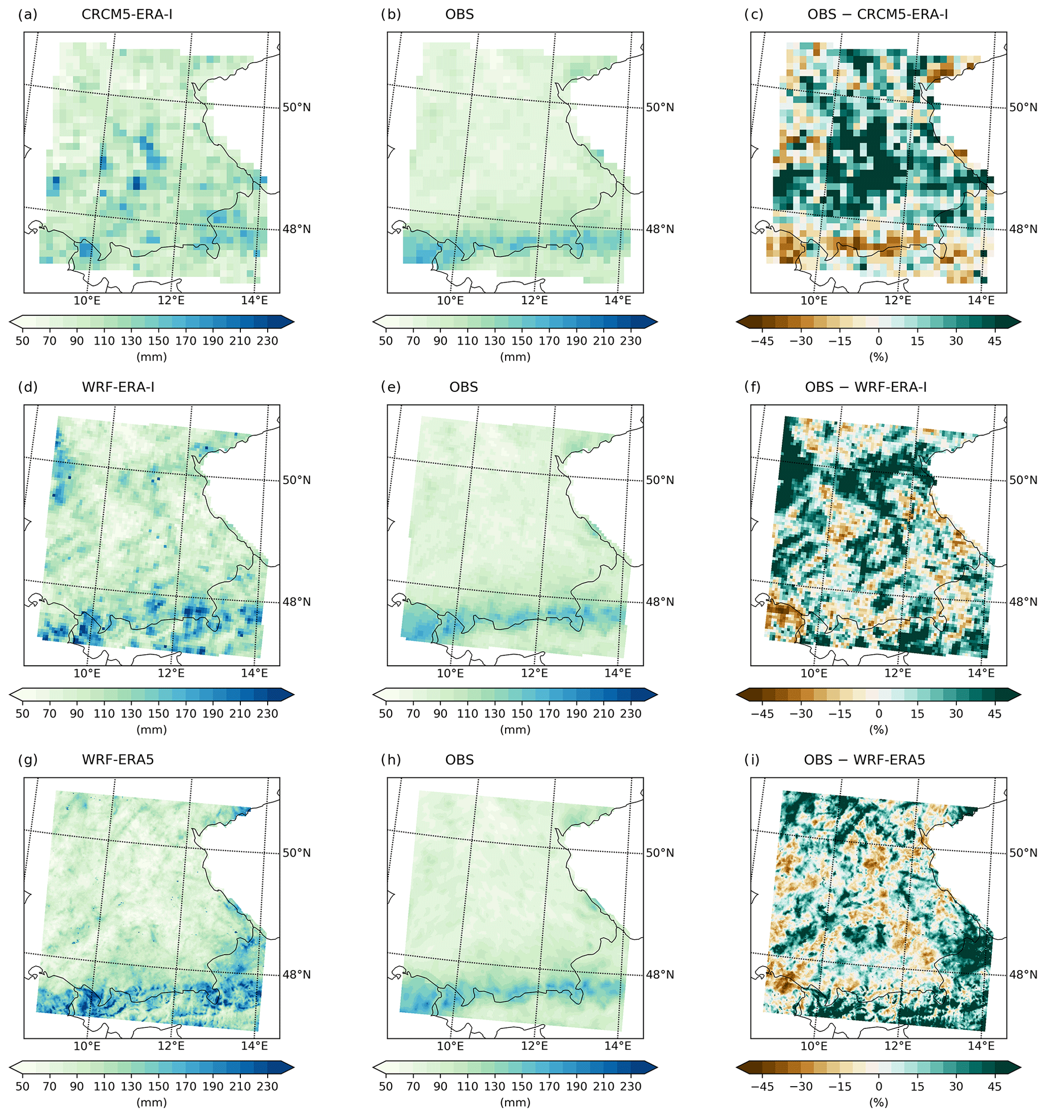
Figure 7The 100-year rainfall return levels applying GEV-LMOM based on CRCM5 ERA-Interim (a), WRF ERA-Interim (d), and WRF ERA5 (g). The middle column (b, e, h) shows the observational product bilinearly interpolated to the respective climate model grid. The right column (c, f, i) provides the percentage difference calculated as the climate model return level minus the observational return level.
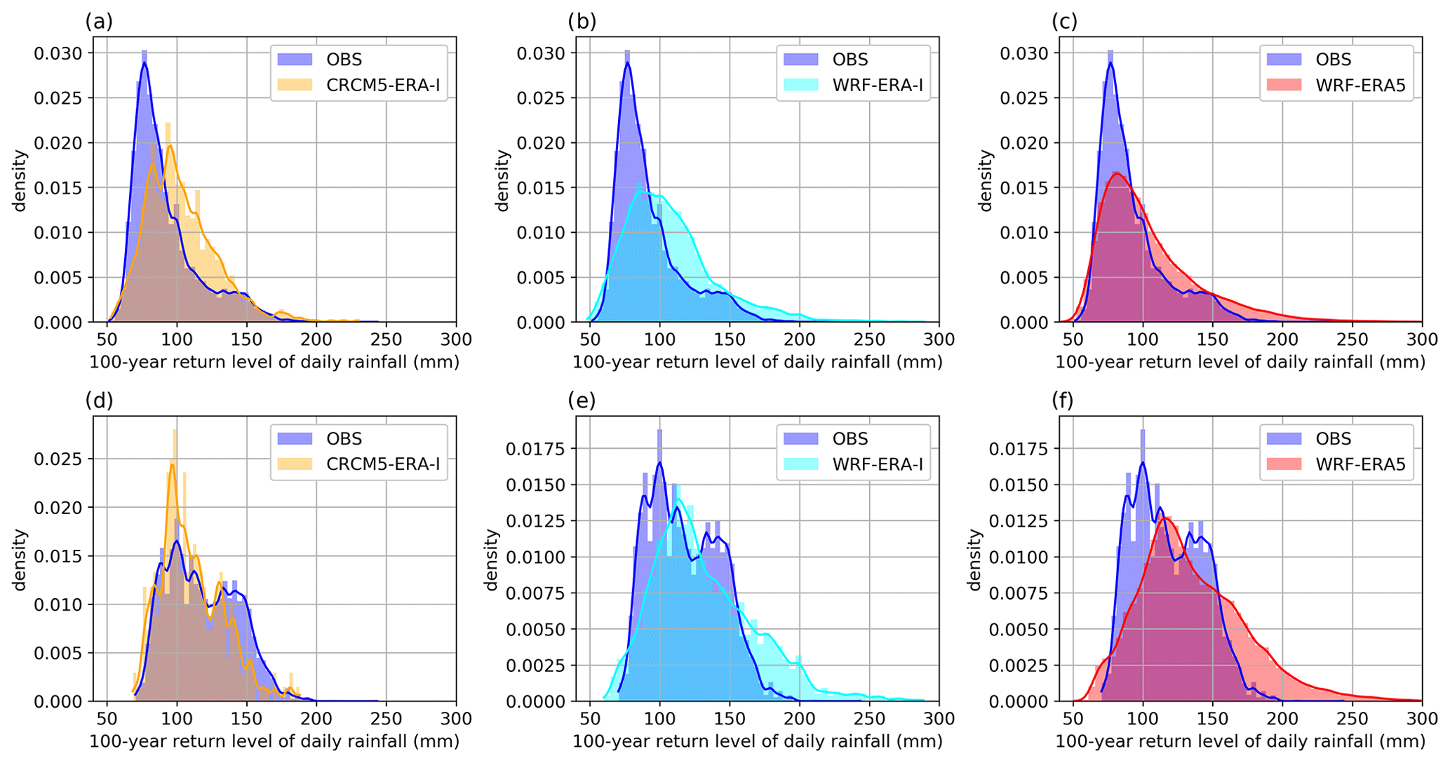
Figure 8Histograms of the resulting 100-year return levels in the whole study area (a–c) and the Alpine area south of 48∘ N (d–f). Gaussian kernel density estimates are plotted to enhance the readability.
Table 3Summary of the applied RCM setups and EVT approaches. Performance metrics of the comparison to observational 100-year return levels are given in terms of the spatially averaged bias and spatial correlation (Spearman). The entries are sorted first by resolution and then by amount of bias.
GEV-LMOM based on WRF ERA-I also suffers from single grid cells with unrealistically high return levels (>200 mm d−1 north of the Alps) due to a high shape parameter (Fig. 3f). The return levels in the areas of all low mountain ranges except the Bavarian Forest are overestimated, especially in the Odenwald in the north-west of the study area (see Fig. 7f). This general overestimation is also visualized in the histogram of Fig. 8b. In the Alps, the 100-year return levels also show the strong orographic signal of WRF ERA-I, leading to a greater variance of return levels than observed (Fig. 8e). The spatial pattern is recreated with ρ=0.55 and the overall bias amounts to 17.8 %.
Applying GEV-LMOM to WRF ERA5 also leads to single grid cells with very high return levels scattered over the study area (Fig. 7g), where the shape parameter is greater than 0.5 (Fig. 3i). Apart from in these locations, the spatial features of the observed 100-year return level are well reproduced (ρ=0.66). On average, the intensities are overestimated (Fig. 8c), amounting to a bias of 13.3 %. In the Alpine area, the simulated rainfall return levels show a greater mean and variance (Fig. 8f).
The application of the further three EVT approaches is shown (Fig. 9) and discussed based on WRF ERA5. The full overview of all climate models and EVT approaches is provided by Figs. 7 and S11–S13. Fixing the shape parameter to ξ=0.114 can eliminate the single grid cells with unrealistic return levels (compare Figs. 7g and 9a). The general spatial pattern is similar; however, GEV-FIX leads to less variance over the whole study area as the shape parameter is restricted to one value. Hence, areas with very low intensities based on GEV-LMOM are higher than those based on GEV-FIX, and high return levels of GEV-LMOM are reduced by GEV-FIX (Figs. 7g and 9a). The comparison to the observational product (Fig. 9c) results in a spatial correlation of ρ=0.70 and an overall bias of 12.9 %.
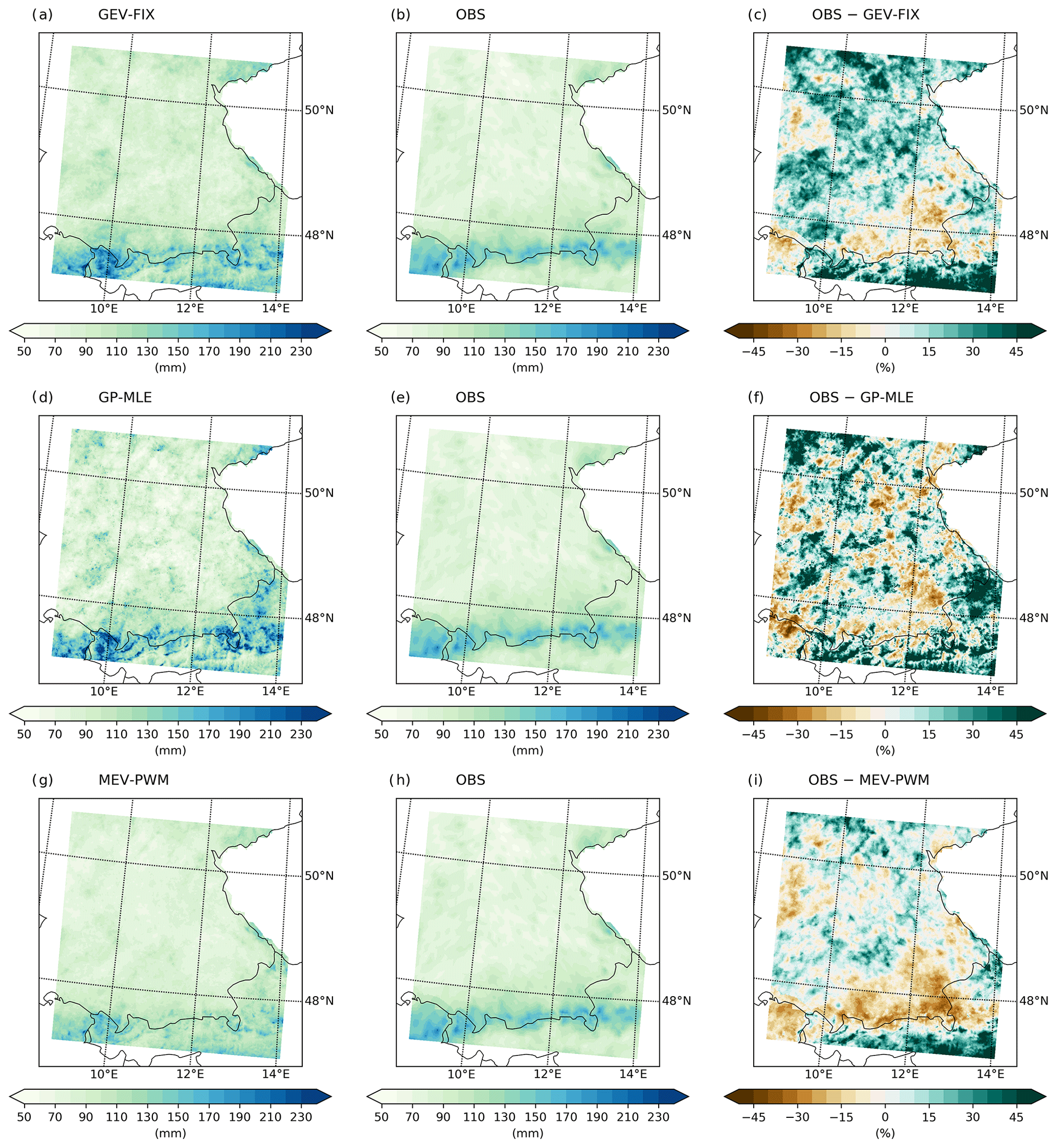
Figure 9The 100-year rainfall return levels based on WRF ERA5 featuring GEV-FIX (a), GP-MLE (d), and MEV-PWM (g). The middle column (b, e, h) shows the observational product interpolated to the WRF-ERA5 grid. The right column (c, f, i) provides the percentage difference calculated as the climate model return level minus the observational return level.
The GP-MLE approach also generates single scattered values with higher intensity, e.g. in the Swabian Jura and in the north-west of the study area (Fig. 9d). These intensities are not as high as for GEV-LMOM, but these cells differ inhomogeneously from their respective neighbouring cells. Generally, the spatial patterns and the range of return level values are similar to those of GEV-LMOM. Hence, the performance metrics in terms of spatial correlation (ρ=0.63) and overall bias (11.9 %) are also close to the metrics of GEV-LMOM.
The 100-year return levels based on the MEV-PWM approach differ from the other EVT approaches in terms of the spatial pattern and rainfall intensities. The spatial pattern north of 48∘ N is very similar to the observations with slight underestimations around the Odenwald and the Prealpine areas in south-eastern Bavaria. However, in the Alpine foreland and on the northern slopes of the Alps, the rainfall intensities are underestimated. In sum, this results in a spatial correlation of ρ=0.73 and an averaged bias of 2.7 %.
Generally, the high values of Spearman's rank correlation as well as the visual comparison to the observational product (Fig. 4) prove that all three RCM setups are able to capture the topographic and climatic differences within the study area. Furthermore, the overall low bias of the 10-year return levels indicates that the complex climate of heavy daily precipitation is reproduced by the climate models. For the 100-year return levels, the choice of the EVT approach has a greater impact on the performance metrics.
Both the overall bias and the spatial correlation of 10- and 100-year return levels imply that the WRF setups at 5 and 1.5 km spatial resolutions can slightly better reproduce the observed return levels than the broader-resolution CRCM5 ERA-I (Tables 2 and 3). There, both WRF setups show similar performance metrics. However, this equivalent performance may be caused by the spatial resolution and spatial representativeness of the observational data (see Fig. S14 for the native resolution). The German dataset is natively resolved at roughly 8 km and the Austrian dataset at 6 km, whereas the Swiss data are given by single gauges interpolated via ordinary kriging. Hence, small-scale spatial features below such resolutions cannot be evaluated by comparison to this observational product. Comparing WRF ERA-I and WRF ERA5 (Figs. 4d, g and 7d, g) reveals a similar spatial pattern, where the more highly resolved WRF ERA5 in particular can add more topographically driven spatial variability in the Alps.
5.1 Uncertainties in the observational datasets
As the German, Austrian, and Swiss data are based on rain gauge measurements, these data are subject to the usual measurement inaccuracies leading to an underestimation of rainfall (Westra et al., 2014). For flat areas in Germany, this deviation is estimated at about 5 % during summer (Richter, 1995). In mountainous areas, this deviation is expected to increase due to higher wind speeds. According to Sevruk (1981), it amounts to 7 % for Switzerland during summer. In addition to these systematic underestimations, different rain gauge types yield varying rainfall measurements, inducing additional uncertainty (Vuerich et al., 2009). This applies to the different meteorological networks in the study area (Kainz et al., 2007; Frei and Schär, 1998; Rauthe et al., 2013; Zolina et al., 2008).
Apart from these measurement errors, the gridded return level products suffer from a limited number of rain gauges (see Sect. 2.2), which also differ in their temporal coverage (Isotta et al., 2014). However, not only the number of stations but also their spatial representativeness is important for an appropriate interpolation from pointwise measurements to gridded estimations (Ahrens, 2006). In mountainous areas, the spatial representativeness of a station is even more limited due to the heterogeneous topography. In addition, the station distribution with elevation is not representative. Due to easier maintenance conditions, more stations are located in valleys than on the tops of the mountains (Ahrens, 2006; Sevruk, 1997), leading to an underestimation for spatially interpolated rainfall in these areas (Isotta et al., 2014). Although the monitoring network density in the Alps makes this one of the best-monitored regions with complex topography, Isotta et al. (2014) estimate the “real” spatial resolution of the observations to be 10–25 km. The regionalization of these pointwise measurements induces additional uncertainties. For the German dataset, the orography is employed as an additional variable to interpolate the return levels (Malitz and Ertel, 2015, following Bartels, 1992). Due to the limited spatial representativeness of the rain gauges in the Alps, the weather model OKM at a 1.5 km resolution (Lorenz and Skoda, 2001) was used to support the spatial interpolation of the Austrian return level data (BMLRT, 2018; Kainz et al., 2007). Thereby, not only the spatial distribution of return levels but also the intensity of the resulting design rainfall return levels was supported by the weather model simulations. The return levels based on observations only are classified as “probably too low” due to the spatial distribution of the rain gauges, whereas the weather model return levels are estimated to be “probably too high” (BMLRT, 2006, 2018). Hence, the resulting design rainfall return level is a weighted averaging combination of the measured rainfall intensities and the intensities simulated by the weather model (BMLRT, 2006). This leads to the conclusion that the deviations of the 10- and 100-year return levels between the WRF setups (see Figs. 4f, i and 7f, i) and the observational data in the Austrian Alps may be caused by the limited spatial representativeness of the measurement stations.
For the Swiss data, ordinary kriging is applied to regionalize the available pointwise return levels. As different interpolation methods yield differing results (Hu et al., 2019), this processing step induces additional uncertainty.
In summary, it can be stated that the study area offers good temporal and spatial coverage of measurements, especially compared to other regions in Europe (Poschlod et al., 2021), which are, however, subject to the uncertainties mentioned above. Additionally, uncertainties due to the application of different EVT approaches contribute to the overall uncertainty and are discussed in Sect. 5.3 as they apply to both observations and climate model data.
Hence, the 10-year return levels (Fig. 4b, e, and h) and 100-year return levels (Fig. 7b, e, and h) provide the best guess based on observations but are still subject to substantial uncertainties, especially in the Alps.
5.2 Uncertainties in the RCM datasets
Generally, climate model simulations of historical conditions are subject to two major uncertainty factors (Hawkins and Sutton, 2009). Due to the chaotic nature of atmospheric processes, the climate system is governed by internal variability. These non-linear dynamics lead to the behaviour of the system where slightly differing starting conditions may result in significantly differing climate realizations (Deser et al., 2012). However, in this study the degree of internal variability is constrained as the RCMs are forced by reanalysis data. The large-scale atmospheric flows are imposed by the lateral boundary conditions, and therefore this source of internal variability is not present in these three RCM setups (Christensen et al., 2001). Still, RCMs are governed by smaller-scale atmospheric variability. Alexandru et al. (2007) have shown that a 20-member RCM ensemble of the CRCM driven by the same lateral boundary conditions with slightly perturbed starting conditions leads to a reasonable spread of simulated precipitation. Even seasonal weather model forecast simulations, which are initialized every month, still show variability, especially for precipitation extremes (Kelder et al., 2020; Thompson et al., 2017). Hence, internal variability cannot be fully excluded as an uncertainty source.
Since models can only represent a simplified image of reality, the structure of climate models leads to the second major uncertainty factor. Even though mainly physically based, RCMs make use of parametrizations with a differing degree of complexity (Jerez et al., 2013). Model uncertainty includes all limitations of the climate model setup such as model-inherent simplifications, parametrizations and schemes, the lateral boundary conditions, nesting, nudging, spin-up times, and spatial resolution.
Multi-model experiments using the same boundary and starting conditions yield deviating simulations of the climate (Holtanová et al., 2019; Solman et al., 2013). Yet the same model applying differing physics options and parametrization schemes can also lead to significant variability in the model results (Laux et al., 2019). Hence, climate model setups can be optimized by choosing different model options and schemes and comparing the simulations to observed climate conditions. For the WRF-ERA-I setup, this has been carried out for the whole domain covering central Europe following Wagner et al. (2018; Warscher et al., 2019). The CRCM5-ERA-I and the WRF-ERA5 setups are based on former applications of the respective climate model in different domains. Adapting the applied options to the study area could potentially improve the model performance (Collier and Mölg, 2020).
Additional uncertainty is induced by the boundary conditions as different reanalysis datasets show considerable deviations from each other (Keller and Wahl, 2021). Here, two different reanalysis datasets at a 75 km (ERA-I) and 30 km (ERA5) spatial resolution covering differing time periods are used to drive the RCMs. Stucki et al. (2020) argue that the difference in the driving conditions regarding the spatial resolution can alter the simulation results, especially over complex terrain.
The different time windows (1980–2009 for ERA-I and 1988–2017 for ERA5) lead to different events being sampled. Due to the small sample size, this variance can also lead to deviations in the resulting return levels.
The overall differences between the three RCM setups indicating model uncertainty are less apparent in the resulting return levels than in the evaluation of individual extreme events. For the close reproduction of extreme rainfall events, Stucki et al. (2020) have shown that initialization of the RCM briefly before the respective events improves the performance at recreating rainfall intensities. Here, the RCMs are run in climate mode featuring transient 30-year simulations (CRCM5 ERA-I, WRF ERA-I) or annual initialization (WRF ERA5). It cannot be expected that single extreme events are closely reproduced due to the internal variability. Hence, such comparison is not appropriate to evaluate the skill of the model but to visualize the differences due to internal variability and model uncertainties. Therefore, the daily rainfall intensities of the two extreme events in May 1999 and August 2005 are given in the Supplement (Figs. S15 and S16). Furthermore, such a comparison makes it clear that the compared setups are climate model setups and not weather model setups, despite the high spatial resolution (Kelder et al., 2020). While the simulation of individual extremes can differ greatly, the 10- and 100-year return levels as a climatic indicator for extreme precipitation show a high degree of agreement (see Figs. 4 and 7). This suggests that despite all the simplifications and differences leading to model uncertainty, the models can reproduce the climatic character of extreme precipitation in the study area.
5.3 Uncertainties due to EVT
The concept of classical EVT (see Sect. 3.1 and 3.2) holds under rather restrictive assumptions (Papalexiou et al., 2013), and each step featuring the choice of the distribution and fitting the distribution parameters induces additional uncertainty (Miniussi and Marani, 2020). For the GEV approach, Eq. (1) holds for a large number of samples n (ideally the sample size n→∞). In practice, the limited available time series make it very difficult to determine whether the distribution of extreme samples is close to its asymptotic GEV limit (Cook and Harris, 2004; Koutsoyiannis, 2004; Miniussi and Marani, 2020).
The POT approach partly overcomes the limitation of very low sample sizes by using the threshold u to define extreme events. However, the choice of this threshold is crucial as the assumptions of a Poisson arrival of exceedances y as well as the GP distribution of these exceedances hold only for a threshold u, ensuring both the sampled events to be extreme and a large number of samples n (Pickands, 1975; Miniussi and Marani, 2020).
Furthermore, uncertainty is induced by the parameter optimization of the respective EVD to adapt the theoretical EVD to the extreme precipitation samples, even though appropriate methods are chosen (see Sect. 3.3; Muller et al., 2009). Assessing the goodness of fit by quality measures or statistical testing (e.g. the Anderson–Darling test) can lower the uncertainty due to the aforementioned assumptions. However, the goodness of fit can only assess the quality of the fit between the theoretical EVD and the empirical distribution of the samples. It cannot evaluate if the samples are a “good representation” of possible extreme rainfall events within the boundaries of internal variability in the climate system.
Uncertainty is therefore apparent as the different sampling approaches, EVDs, and fitting methods may lead to differing estimations of rainfall return levels (Lazoglou and Anagnostopoulou, 2017). For GEV-LMOM (Fig. 4g) and GP-MLE (Fig. 6d) based on WRF ERA5, the mean absolute deviation (MAD) between the 10-year return levels based on both approaches amounts to a spatial average of 1.7 %. The MAD between the respective 100-year return levels amounts to 8.0 %. Hence, despite different sampling, distributions, and fitting methods, the results are close to each other on average. Larger deviations occur at single grid cells.
However, both classical approaches still suffer from drawbacks. Papalexiou and Koutsoyiannis (2013) as well as Serinaldi and Kilsby (2014) argue that producing stable fits of the shape parameter of the GEV and GP distributions needs larger sample sizes than are typically available. They have shown that the estimation of the shape parameter of the GEV and GP distributions is dependent on the sample size, whereby it is also influenced by the geographical location. Papalexiou and Koutsoyiannis (2013) propose to restrict the shape parameter of the GEV to a window described by a normal distribution around the mean value of 0.114 or to apply a fixed shape parameter of ξ=0.114. Indeed, the shape parameter of GEV-LMOM shows a heterogeneous spatial distribution with small patches of positive and negative values for all three RCM setups (Fig. 3c, f, and i). This spatial distribution can be interpreted as “noise” due to sample sizes that are too small, where the 30 annual maximum precipitation events do not fully represent the range of possible extreme precipitation within the boundaries of internal climate variability. The distribution of the shape parameter ξ based on all three RCM setups is centred around a value close to 0.114 (see Fig. S1c). However, Papalexiou and Koutsoyiannis (2013) suggest that 99 % of the distribution should be between 0 and 0.225, whereas the distribution of all three RCM setups reveals a larger spread. When restricting the shape parameter to ξ=0.114, however, the 10-year return levels only differ very slightly from those of GEV-LMOM, resulting in an average MAD of 3.4 % (see Fig. 6a). As ξ only defines the tail of the distribution, it is more relevant for longer return periods. Hence, high values of the shape parameter (Fig. 3c, f, and i) strongly influence the resulting 100-year return level. The outcome of this issue shows up as unrealistically high rainfall intensities (Fig. 7a, d, and g) at single grid cells. The GP-MLE approach also suffers from this problem to a lesser extent (Fig. 9d). The fixed shape parameter prevents this issue (Figs. 9a and S11). However, restricting the shape parameter also restricts the flexibility of the GEV, which results in a smaller range of 100-year return levels. The low return levels in the plains and leeward areas are therefore slightly overestimated. However, the resulting 100-year return levels show a higher degree of homogeneity than the 100-year return levels of GEV-LMOM or GP-MLE (compare Fig. 9a to Figs. 7g and 9d).
In addition to unstable parameters fits, the sampling strategies of both classical EVT approaches only use a small fraction of available data. In this study, only 0.3 % (GEV) and 0.8 % (GP) of the daily precipitation sums from the RCMs are sampled. Especially with respect to short available observation time series but also with respect to the extensive computational power and related costs of such high-resolution climate models, this sampling is a waste of valuable information (Miniussi and Marani, 2020). The sampling of the MEV approach overcomes this limitation and uses the information of rainfall intensities of all wet days as well as the frequency of these days. This is found to result in more stable fits (Zorzetto et al., 2016). Zorzetto et al. (2016) concluded that the MEV outperforms the classical GEV approach due to the more stable parameter fits if the return period exceeds the length of the available samples. Furthermore, they found that the MEV is better than the GEV at predicting return levels if the EVT models are calibrated on samples that are independent from the samples used to calculate the return levels. In this study, the MEV-PWM return levels are on average lower than the return levels based on the other EVT approaches (Tables 2 and 3). While this leads to an average underestimation of the observational product at the 10-year return levels, the MEV can outperform the other EVT approaches at the 100-year return levels. In terms of the spatial correlation, MEV-PWM leads to superior results overall than the other approaches for both calculated return levels. The moderate to strong underestimation of rainfall intensities at the 100-year return period in the area of the Prealps and northern Alps (Fig. 9i) is mainly attributed to the climate model data, as all EVT approaches yield lower intensities in this area as well (Figs. 7i, 9c and f). The other EVT approaches “compensate” for these low intensities by their tendency to overestimate the 100-year return levels (see Figs. 7i and 9). Schellander et al. (2019) apply the MEV optimized via the PWM method and GEV optimized via MLE to 55 rain gauges with more than 100 years of measurements in Austria, which is partly covered by the study area. They split the data, and up to 50 years is used to calibrate the EVT models. The remaining data are the basis to calculate the return levels, which are used for the evaluation of the GEV and MEV. They find that the MEV can outperform the GEV for return periods of 30 years or longer when less than 30 years of data is available. For the two cases of this study (sample size of 30 years and return periods of 10 and 100 years), they report a slightly superior performance of the GEV for 10-year return levels and a slightly superior performance of the MEV for 100-year return levels. In sum, the results of their study are in line with the findings of this study, even if the differences between GEV and MEV in this investigation are a little more pronounced, especially for the 100-year return period.
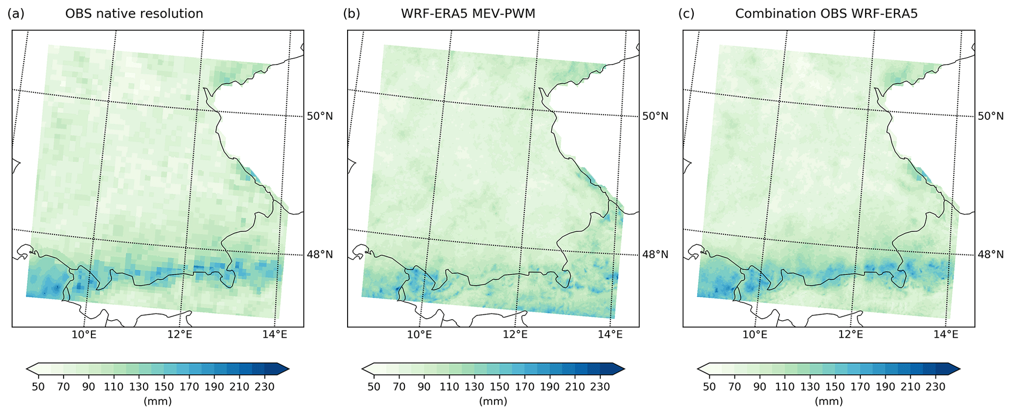
Figure 10(a) Observational 100-year return levels based on the German (8 km), Austrian (6 km), and Swiss (interpolated via ordinary kriging) data at the original resolution. (b) The 100-year return levels based on WRF ERA5 applying the MEV-PWM approach. (c) Combination of (a) and (b) by applying a Gaussian filter to the differences.
Various combinations of high-resolution regional climate models driven by reanalysis data and state-of-the-art EVT approaches have been explored to reproduce 10- and 100-year return levels of daily rainfall. The 5 km WRF-ERA-I setup reveals added value in terms of spatial correlation and bias compared to the lower-resolution 12 km CRCM5 ERA-I. The very high resolution 1.5 km WRF ERA5, accompanied by an explicit simulation of convective processes, can only slightly improve the performance metrics. This is possibly since the observational product is resolved natively between 6 and 8 km. Hence finer-scale spatial features cannot be evaluated by such comparison. Despite the improvement in overall performance metrics, local biases on the order of 30 % to 40 % still remain. Therefore, the criticism of the practitioners that was expressed for the CRCM5 return levels from Poschlod et al. (2021; see Sect. 1) would also be present for the return levels shown here.
The resulting 10-year return levels based on the four different EVT approaches applied show good agreement with each other and with the observational product. This suggests that the methodological uncertainty for return levels of moderate extremes is relatively low. However, if return periods outside the sample size are to be extrapolated, the estimation uncertainty in the shape parameter governing the tail of the GEV and GP distributions becomes more important. The 100-year return levels based on GEV-LMOM and GP-MLE suffer from single grid cells with unrealistically high return levels due to high estimations of the shape parameter. Two approaches are studied to overcome this uncertainty. The GEV with a fixed shape parameter shows 100-year return levels, and its performance metrics are almost equivalent to the three-parameter GEV optimized via L-moments. However, the resulting return levels are homogeneous and do not show any unrealistic outliers. The rather new EVT approach by Marani and Ignaccolo (2015) featuring the MEV distribution leads to a slight underestimation of 10-year return levels but produces the best results for the 100-year return period. This methodology shows great potential for the extrapolation of longer return periods due to the larger sampling and, therefore, increased stability of the fits (Schellander et al., 2019; Zorzetto et al., 2016).
The question remains to be answered as to what the findings of this study can contribute to in practice.
First, in regions with a low density of rain gauges, such RCM setups can contribute to a homogeneous spatial estimation of return levels. Even in regions where the rain gauges cannot represent the spatial heterogeneity, RCMs can be applied to support observational products. This is already being done in Austria using a convective-permitting weather model, and the results of this study reinforce such use of regional climate models. It is also conceivable to use the high-resolution spatial patterns of CPMs as an auxiliary variable for the interpolation of the return levels based on measured data (e.g. via kriging with external drift – Haberlandt, 2007; spatial GEV models – Davison et al., 2012; or a spatial representation of the simplified MEV – Schellander et al., 2019). A visualization of a simple combination approach for such a subsequent enhancement of 100-year return levels is provided in Fig. 10. Therein, the differences at each grid cell between the observational product and the WRF-ERA5 MEV-PWM results are smoothed with a Gaussian filter and again added to the climate model return levels. However, this rather naive approach only serves to provide a visual impression of a possible enhancement.
Second, different EVT approaches are explored based on 30 years of data with daily rainfall. For moderate extremes (10-year return level), the differences between the EVT approaches are minor. Due to the slight underestimation of the MEV-PWM, GEV and GP approaches can be recommended for such applications. For return periods that are longer than the available data coverage, the estimation uncertainty in the shape parameter of the GEV and GP distributions induces unrealistic return level values at single grid cells. Fixing the shape parameter can prevent this issue. However, the MEV framework using the information of all ordinary wet events produces stable fits and shows the best performance at the reproduction of 100-year return levels. It is recommended for applications where the return period needs to be extrapolated.
Further conclusions regarding the future use of RCMs follow from these findings. Third, large ensembles of RCMs can be set up to increase the sample size within the boundaries of the internal climate variability. On the one hand, increased sample sizes lower the uncertainty related to EVT; on the other hand large ensembles enable the quantification of uncertainties due to internal variability (Poschlod et al., 2021).
Fourth, RCMs driven by global climate models following different emission scenarios allow the simulation of climate-change-induced alterations of return levels (Ban et al., 2020; Poschlod and Ludwig, 2021). Even though an increase in extreme precipitation intensities has been known about for decades (Trenberth et al., 2003), there is a lack of operational implementation and adaptation. In 2004, a climate change surcharge of a flat +15 % on top of the 100-year flood return level was introduced in Bavaria for the planning of flood protection facilities (LfU, 2021). Indeed, trends in the magnitude of floods in Bavaria can be detected (Blöschl et al., 2019). However, such an adaptation for extreme rainfall has been missing so far, even though there is a much higher consensus in the scientific community about the increase in extreme rainfall intensities than about the increase in floods (Sharma et al., 2018; Merz et al., 2021).
Despite all model-specific uncertainties, the evaluation of RCMs in this study proved that they are suitable for reproducing daily extreme precipitation intensities over complex terrain.
The observational rainfall return level data are available at the German weather service (https://opendata.dwd.de/climate_environment/CDC/grids_germany/return_periods/precipitation/KOSTRA/KOSTRA_DWD_2010R/asc/, DWD, 2020), the Austrian Federal Ministry of Agriculture, Regions and Tourism (https://ehyd.gv.at/, BMLRT, 2020), and MeteoSwiss (https://www.meteoswiss.admin.ch/home/climate/swiss-climate-in-detail/extreme-value-analyses/standard-period.html?station=int, MeteoSwiss, 2021).
The daily precipitation of WRF ERA-I and WRF ERA5 is publicly available in Warscher (2019, https://doi.org/10.5281/zenodo.2533904) and Collier (2020, https://doi.org/10.17605/OSF.IO/AQ58B), who are cordially acknowledged. The CRCM5-ERA-I data are available at https://climex-data.srv.lrz.de/Public/ERA_driven_run/pr/ (ClimEx, 2021).
The supplement related to this article is available online at: https://doi.org/10.5194/nhess-21-3573-2021-supplement.
The author declares that there is no conflict of interest.
Publisher's note: Copernicus Publications remains neutral with regard to jurisdictional claims in published maps and institutional affiliations.
I cordially thank all data providers for the open access to their data. Further, I thank all members of the ClimEx project working group for their contributions to produce the CRCM5 dataset. The ClimEx project is funded by the Bavarian State Ministry of the Environment and Consumer Protection. The CRCM5 was developed by the ESCER centre of the Université du Québec a Montréal in collaboration with Environment and Climate Change Canada. Computations with the CRCM5 for the ClimEx project were made on the SuperMUC supercomputer at the Leibniz Supercomputing Centre of the Bavarian Academy of Sciences and Humanities. The operation of this supercomputer is funded via the Gauss Centre for Supercomputing by the German Federal Ministry of Education and Research and the Bavarian State Ministry of Science and the Arts.
This research has been supported by the Bayerisches Landesamt für Umwelt (grant no. 81-0270-82467/2019).
This paper was edited by Joaquim G. Pinto and reviewed by two anonymous referees.
Ahrens, B.: Distance in spatial interpolation of daily rain gauge data, Hydrol. Earth Syst. Sci., 10, 197–208, https://doi.org/10.5194/hess-10-197-2006, 2006.
Alexandru, A., Elia, R. D., and Laprisé, R.: Internal Variability in Regional Climate Downscaling at the Seasonal Scale, Mon. Weather Rev., 135, 3221–3238, https://doi.org/10.1175/MWR3456.1, 2007.
Balkema, A. A. and de Haan, L.: Residual life time at great age, Ann. Probab., 2, 792–804, 1974.
Ban, N., Rajczak, J., Schmidli, J., and Schär, C.: Analysis of Alpine precipitation extremes using generalized extreme value theory in convection-resolving climate simulations, Clim. Dynam., 55, 61–75, https://doi.org/10.1007/s00382-018-4339-4, 2020.
Barbero, R., Fowler, H. J., Blenkinsop, S., Westra, S., Moron, V., Lewis, E., Chan, S., Lenderink, G., Kendon, E., Guerreiro, S., Li, X.-F., Villalobos, R., Ali, H., and Mishra, V.: A synthesis of hourly and daily precipitation extremes in different climatic regions, Weather. Clim. Ext., 26, 100219, https://doi.org/10.1016/j.wace.2019.100219, 2019.
Bartels, H.: Regionalisierung am Beispiel der flächendeckenden Starkniederschlagsauswertung für die Bundesrepublik Deutschland, in: Regionalisierung in der Hydrologie, DFG, Mitteilung XI der Senatskommission für Wasserforschung, Weinheim, Germany, 1992.
Bélair, S., Mailhot, J., Girard, C., and Vaillancourt, P.: Boundary layer and shallow cumulus clouds in a medium-range forecast of a large-scale weather system, Mon. Weather Rev., 133, 1938–1960, https://doi.org/10.1175/MWR2958.1, 2005.
Benjamin, D. M. and Budescu, D. V.: The Role of Type and Source of Uncertainty on the Processing of Climate Models Projections, Front. Psychol., 9, 403, https://doi.org/10.3389/fpsyg.2018.00403, 2018.
Benjamini, Y. and Hochberg, Y.: Controlling the false discovery rate – a practical and powerful approach to multiple testing, J. Roy. Stat. Soc. B, 57, 289–300, https://doi.org/10.1111/j.2517-6161.1995.tb02031.x, 1995.
Berg, P., Christensen, O. B., Klehmet, K., Lenderink, G., Olsson, J., Teichmann, C., and Yang, W.: Summertime precipitation extremes in a EURO-CORDEX 0.11∘ ensemble at an hourly resolution, Nat. Hazards Earth Syst. Sci., 19, 957–971, https://doi.org/10.5194/nhess-19-957-2019, 2019.
Berghuijs, W. R., Harrigan, S., Molnar, P., Slater, L. J., and Kirchner, J. W.: The Relative Importance of Different Flood-Generating Mechanisms Across Europe, Water Resour. Res., 55, 4582–4593, https://doi.org/10.1029/2019WR024841, 2019.
BLFW – Bayerisches Landesamt für Wasserwirtschaft: Hochwasser Mai 1999 Gewässerkundliche Beschreibung, Tech. Rep., Munich, Germany, 44 pp., 2003.
Blöschl, G., Hall, J., Parajka, J., Perdigão, R. A. P., Merz, B., Arheimer, B., Aronica, G. T., Bilibashi, A., Bonacci, O., Borga, M., Čanjevac, I., Castellarin, A., Chirico, G. B., Claps, P., Fiala, K., Frolova, N., Gorbachova, L., Gül, A., Hannaford, J., Harrigan, S., Kireeva, M., Kiss, A., Kjeldsen, T. R., Kohnová, S., Koskela, J. J., Ledvinka, O., Macdonald, N., Mavrova-Guirguinova, M., Mediero, L., Merz, R., Molnar, P., Montanari, A., Murphy, C., Osuch, M., Ovcharuk, V., Radevski, I., Rogger, M., Salinas, J. L., Sauquet, E., Šraj, M., Szolgay, J., Viglione, A., Volpi, E., Wilson, D., Zaimi, K., and Živković, N.: Changing climate both increases and decreases European river floods, Nature, 573, 108–111, https://doi.org/10.1038/s41586-019-1495-6, 2019.
BMLRT – Bundesministerium für Landwirtschaft, Regionen und Tourismus: Forschungsprojekt “Bemessungsniederschläge in der Siedlungswasserwirtschaft”, Tech. Rep., Vienna, Austria, 79 pp., 2006.
BMLRT – Bundesministerium für Landwirtschaft, Regionen und Tourismus: eHyd Auswertungen Karte Bemessungsniederschlag, Tech. Rep., Vienna, Austria, 10 pp., 2018.
BMLRT – Bundesministerium für Landwirtschaft, Regionen und Tourismus: eHYD, BMLRT [data set], https://ehyd.gv.at/, last access: 22 January 2020.
Boughton, W. and Jakob, D.: Adjustment factors for restricted rainfall, Aust. J. Water Resour., 12, 37–47, https://doi.org/10.1080/13241583.2008.11465332, 2008.
Breinl, K., Müller-Thomy, H., and Blöschl, G.: Space–Time Characteristics of Areal Reduction Factors and Rainfall Processes, J. Hydrometeorol., 21, 671–689, https://doi.org/10.1175/JHM-D-19-0228.1, 2020.
Brisson, E., Van Weverberg, K., Demuzere, M., Devis, A., Saeed,S., Stengel, M., and van Lipzig, N. P. M.: How well can a convection-permitting climate model reproduce decadal statistics of precipitation, temperature and cloud characteristics?, Clim. Dynam., 47, 3043–3061, https://doi.org/10.1007/s00382-016-3012-z, 2016.
Bücher, A., Lilienthal, J., Kinsvater, P., and Fried, R.: Penalized quasi-maximum likelihood estimation for extreme value models with application to flood frequency analysis, Extremes, 24, 325–348, https://doi.org/10.1007/s10687-020-00379-y, 2021.
Chen, K.-F. and Leandro, J.: A Conceptual Time-Varying Flood Resilience Index for Urban Areas: Munich City, Water, 11, 830, https://doi.org/10.3390/w11040830, 2019.
Christensen, O. B., Gaertner, M. A., Prego, J. A., and Polcher, J.: Internal variability of regional climate models, Clim. Dynam., 17, 875–887, https://doi.org/10.1007/s003820100154, 2001.
ClimEx: CLIMEX data access to public data, ClimEx [data set], available at: https://climex-data.srv.lrz.de/Public/ERA_driven_run/pr/, last access: 11 February 2021.
Coles, S.: An introduction to statistical modeling of extreme values, Springer, London, UK, 2001.
Collier, E.: BAYWRF, OSFHOME [data set], https://doi.org/10.17605/OSF.IO/AQ58B, 2020.
Collier, E. and Mölg, T.: BAYWRF: a high-resolution present-day climatological atmospheric dataset for Bavaria, Earth Syst. Sci. Data, 12, 3097–3112, https://doi.org/10.5194/essd-12-3097-2020, 2020.
Collier, E., Sauter, T., Mölg, T., and Hardy, D.: The influence of tropical cyclones on circulation, moisture transport, and snow accumulation at Kilimanjaro during the 2006–2007 season, J. Geophys. Res.-Atmos., 124, 6919–6928, https://doi.org/10.1029/2019JD030682, 2019.
Cook, N. J. and Harris, R. I.: Exact and general FT1 penultimate distributions of extreme wind speeds drawn from tail-equivalent Weibull parents, Struct. Saf., 26, 391–420, https://doi.org/10.1016/j.strusafe.2004.01.002, 2004.
Coppola, E., Sobolowski, S., Pichelli, E., Raffaele, F., Ahrens, B., Anders, I., Ban, N., Bastin, S., Belda, M., Belušić, D., Caldas-Alvarez, A., Cardoso, R. M., Davolio, S., Dobler, A., Fernandez, J., Fita, L., Fumiere, Q., Giorgi, F., Goergen, K., Güttler, I., Halenka, T., Heinzeller, D., Hodnebrog, Ø., Jacob, D., Kartsios, S., Katragkou, E., Kendon, E., Khodayar, S., Kunstmann, H., Knist, S., Lavín-Gullón, A., Lind, P., Lorenz, T., Maraun, D., Marelle, L., van Meijgaard, E., Milovac, J., Myhre, G., Panitz, H.-J., Piazza, M., Raffa, M., Raub, T., Rockel, B., Schär, C., Sieck, K., Soares, P. M. M., Somot, S., Srnec, L., Stocchi, P., Tölle, M. H., Truhetz, H., Vautard, R., de Vries, H., and Warrach-Sagi, K.: A first-of-its-kind multi-model convection permitting ensemble for investigating convective phenomena over Europe and the Mediterranean, Clim. Dynam., 55, 3–34, https://doi.org/10.1007/s00382-018-4521-8, 2020.
Davison, A. C. and Smith, R. L.: Models for exceedances over high thresholds, J. Roy. Stat. Soc., 52, 393–442, 1990.
Davison, A. C., Padoan, S. A., and Ribatet, M.: Statistical modelling of spatial extremes, Stat. Sci., 27, 161–186, https://doi.org/10.1214/11-STS376, 2012.
Dee, D. P., Uppala, S. M., Simmons, A. J., Berrisford, P., Poli,P, Kobayashi, S., Andrae, U., Balmaseda, M. A., Balsamo, G., Bauer, P., Bechtold, P., Beljaars, A. C. M., van de Berg, L., Bid-lot, J., Bormann, N., Delsol, C., Dragani, R., Fuentes, M., Geer, A. J., Haimberger, L., Healy, S. B., Hersbach, H., Hólm, E. V.,Isaksen, L., Kallberg, P., Köhler, M., Matricardi, M., McNally, A. P., Monge-Sanz, B. M., Morcrette, J.-J., Park, B.-K., Peubey,C., de Rosnay, P., Tavolato, C., Thépaut, J.-N., and Vitart, F.: The ERA-Interim reanalysis: configuration and performance of the data assimilation system, Q. J. Roy. Meteorol. Soc., 137, 553–597, https://doi.org/10.1002/qj.828, 2011.
Delicado, P. and Goria, M. N.: A small sample comparison of maximum likelihood, moments and l-moments methods for the asymmetric exponential power distribution, Comput. Stat. Data Anal., 52, 1661–1673, https://doi.org/10.1016/j.csda.2007.05.021, 2008.
Deser, C., Phillips, A., Bourdette, V., and Teng, H.: Uncertainty in climate change projections: the role of internal variability, Clim. Dynam., 38, 527–546, https://doi.org/10.1007/s00382-010-0977-x, 2012.
DWD – Deutscher Wetterdienst: KOSTRA_DWD_2010R, DWD [data set], https://opendata.dwd.de/climate_environment/CDC/grids_germany/return_periods/precipitation/KOSTRA/KOSTRA_DWD_2010R/asc/, last access: 21 October 2020.
DWD – Deutscher Wetterdienst: Klimaatlas, https://www.dwd.de/DE/klimaumwelt/klimaatlas/klimaatlas_node.html, last access: 10 February 2021.
Ehmele, F. and Kunz, M.: Flood-related extreme precipitation in southwestern Germany: development of a two-dimensional stochastic precipitation model, Hydrol. Earth Syst. Sci., 23, 1083–1102, https://doi.org/10.5194/hess-23-1083-2019, 2019.
Fisher, R. A. and Tippett, L. H. C.: Limiting forms of the frequency distribution of the largest or smallest member of a sample, Math. Proc. Cambr. Phil. Soc., 24, 180–190, https://doi.org/10.1017/S0305004100015681, 1928.
Fosser, G., Khodayar, S., and Berg, P.: Benefit of convection permitting climate model simulations in the representation of convective precipitation, Clim. Dynam., 44, 45–60, https://doi.org/10.1007/s00382-014-2242-1, 2014.
Frei, C. and Schär, C.: A precipitation climatology of the Alps from high-resolution rain-gauge observations, Int. J. Climatol., 18, 873–900, https://doi.org/10.1002/(SICI)1097-0088(19980630)18:8<873::AID-JOC255>3.0.CO;2-9, 1998.
Fukutome, S., Schindler, A., and Capobianco, A.: MeteoSwiss extreme value analyses: User manual and documentation, Technical Report MeteoSwiss 255, 3rd Edn., Zurich, Switzerland, 80 pp., 2015.
Gilleland, E., and Katz, R. W.: extRemes 2.0: An Extreme Value Analysis Package in R, J. Stat. Softw., 72, 8, https://doi.org/10.18637/jss.v072.i08, 2016.
Gilleland, E., Katz, R. W., and Naveau, P.: Quantifying the Risk of Extreme Events under Climate Change, CHANCE, 30, 4, 30–36, https://doi.org/10.1080/09332480.2017.1406757, 2017.
Gnedenko, B.: Sur la distribution limite du terme maximum d'uneserie aleatoire, Ann. Math., 44, 423–453, 1943.
Goda, Y.: Inherent negative bias of quantile estimates of annual maximum data due to sample size effect: A numerical simulation study, Coast. Eng. J., 53, 397–429, https://doi.org/10.1142/S0578563411002409, 2011.
Goudenhoofdt, E. and Delobbe, L.: Generation and Verification of Rainfall Estimates from 10-Yr Volumetric Weather Radar Measurements, J. Hydrometeorol., 17, 1223–1242, https://doi.org/10.1175/JHM-D-15-0166.1, 2016.
Greenwood, J., Landwehr, J., and Matalas, N.: Probability weighted moments: Definition and relation to parameters of several distributions expressable in inverse form, Water Resour. Res., 15, 1049–1054, https://doi.org/10.1029/WR015i005p01049, 1979.
Grell, G. A. and Freitas, S. R.: A scale and aerosol aware stochastic convective parameterization for weather and air quality modelling, Atmos. Chem. Phys, 14, 5233–5250, https://doi.org/10.5194/acp-14-5233-2014, 2014.
Grieser, J., Beck, C., and Rudolf, B.: The Summer Flooding 2005 in Southern Bavaria – A Climatological Review, in: Klimastatusbericht 2005, edited by: Deutscher Wetterdienst, Offenbach a. M., Germany, 168–173, 2006.
Gutowski, W. J., Decker, S. G., Donavon, R. A., Pan, Z. T., Arritt, R. W., and Takle, E. S.: Temporal-spatial scales of observed and simulated precipitation in central U.S. climate, J.Climate, 16, 3841–3847, https://doi.org/10.1175/1520-0442(2003)016<3841:tsooas>2.0.co;2, 2003.
Haberlandt, U.: Geostatistical interpolation of hourly precipitation from rain gauges and radar for a large scale extreme rainfall event, J. Hydrol., 332, 144–157, https://doi.org/10.1016/j.jhydrol.2006.06.028, 2007.
Hawkins, E. and Sutton, R.: The potential to narrow uncertainty in regional climate predictions, B. Am. Meteorol. Soc., 90, 1095–1108, https://doi.org/10.1175/2009BAMS2607.1, 2009.
Haylock, M. R., Hofstra, N., Klein Tank, A. M. G., Klok, E. J., Jones, P. D., and New, M.: A European daily high-resolution gridded data set of surface temperature and precipitation for 1950–2006, J. Geophys. Res., 113, D20119, https://doi.org/10.1029/2008JD010201, 2008.
Heo, J.-H., Salas, J. D., and Kim, K.-D.: Estimation of confidence intervals of quantiles for the Weibull distribution, Stoch. Environ. Res. Risk A., 15, 284–309, https://doi.org/10.1007/s004770100071, 2001.
Hernández-Díaz, L., Laprise, R., Sushama, L., Martynov, A., Winger, K., and Dugas, B.: Climate simulation over the CORDEX-Africa domain using the fifth-generation Canadian Regional Climate Model (CRCM5), Clim. Dynam., 40, 1415–1433, https://doi.org/10.1007/s00382-012-1387-z, 2012.
Hersbach, H., Bell, B., Berrisford, P., Hirahara, S., Horányi, A., Muñoz-Sabater, J., Nicolas, J., Peubey, C., Radu, R., Schepers, D., Simmons, A., Soci, C., Abdalla, S., Abellan, X., Balsamo, G., Bechtold, P., Biavati, G., Bidlot, J., Bonavita, M., Chiara, G. D., Dahlgren, P., Dee, D., Diamantakis, M., Dragani, R., Flemming, J., Forbes, R., Fuentes, M., Geer, A., Haimberger, L., Healy, S., Hogan, R. J., Hólm, E., Janisková, M., Keeley, S., Laloyaux, P., Lopez, P., Lupu, C., Radnoti, G., de Rosnay, P., Rozum, I., Vamborg, F., Villaume, S., and Thépaut, J.-N.: The ERA5 Global Reanalysis, Q. J. Roy. Meteorol. Soc., 146, 1999–2049, https://doi.org/10.1002/qj.3803, 2020.
Hofstätter, M., Lexer, A., Homann, M., and Blöschl, G.: Large-scale heavy precipitation over central Europe and the role of atmospheric cyclone track types, Int. J. Climatol., 38, e497–e517, https://doi.org/10.1002/joc.5386, 2018.
Holtanová, E., Mendlik, T., Koláček, J., Horová, I., and Mikšovský, J.: Similarities within a multi-model ensemble: functional data analysis framework, Geosci. Model Dev., 12, 735–747, https://doi.org/10.5194/gmd-12-735-2019, 2019.
Hong, Y., Hsu, K.-L., Sorooshian, S., and Gao, X.: Precipitation estimation from remotely sensed imagery using an artificial neural network cloud classification system, J. Appl. Meteorol., 43, 1834–1853, https://doi.org/10.1175/JAM2173.1, 2004.
Hosking, J. R. M., Wallis, J. R., and Wood, E. F.: Estimation of the Generalized Extreme-Value Distribution by the Method of Probability-Weighted Moments, Technometrics, 27, 251–261, https://doi.org/10.1080/00401706.1985.10488049, 1985.
Hu, G. and Franzke, C. L. E.: Evaluation of daily precipitation extremes in reanalysis and gridded observation-based data sets over Germany, Geophys. Res. Lett., 47, e2020GL089624, https://doi.org/10.1029/2020GL089624, 2020.
Hu, Q., Li, Z., Wang, L., Huang, Y., Wang, Y., and Li, L.: Rainfall Spatial Estimations: A Review from SpatialInterpolation to Multi-Source Data Merging, Water, 11, 579, https://doi.org/10.3390/w11030579, 2019.
Isotta, F. A., Frei, C., Weilguni, V., Tadić, M. P., Lassègues, P., Rudolf, B., Pavan, V., Cacciamani, C., Antolini, G., Ratto, S. M., Munari, M., Micheletti, S., Bonati, V., Lussana, C., Ronchi, C., Panettieri, E., Marigo, G., and Vertačnik, G.: The climate of daily precipitation in the Alps: development and analysis of a high-resolution grid dataset from pan-Alpine rain-gauge data, Int. J. Climatol., 34, 1657–1675, https://doi.org/10.1002/joc.3794, 2014.
Jarvis, A., Reuter, H. I., Nelson, A., and Guevara, E.: Hole-filled SRTM for the globe Version 4, CGIAR-CSI [data set], available at: https://srtm.csi.cgiar.org/, last access: 28 January 2021.
Jerez, S., Montavez, J. P., Gomez-Navarro, J. J., Lorente-Plazas, R., Garcia-Valero, J. A., and Jimenez-Guerrero, P.: A multi-physics ensemble of regional climate change projections over the Iberian Peninsula, Clim. Dynam., 41, 1749–1768, https://doi.org/10.1007/s00382-012-1551-5, 2013.
Joyce, R. J., Janowiak, J. E., Arkin, P. A., and Xie, P.: CMORPH: A 680 method that produces global precipitation estimates from passive microwave and infrared data at high spatial and temporal resolution, J. Hydrometeorol., 5, 487–503, https://doi.org/10.1175/1525-7541(2004)005h0487:CAMTPGi2.0.CO;2, 2004.
Junghänel, T., Ertel, H., and Deutschländer, T.: Bericht zur Revision der koordinierten Starkregenregionalisierung und -auswertung des Deutschen Wetterdienstes in der Version 2010, Tech. Rep., Deutscher Wetterdienst, Offenbach a. M., Germany, 30 pp., 2017.
Kain, J. S. and Fritsch, J. M.: A one-dimensional entraining/detraining plume model and its application in convective parameterization, J. Atmos. Sci., 47, 2784–2802, https://doi.org/10.1175/1520-0469(1990)047<2784:AODEPM>2.0.CO;2, 1990.
Kainz, H., Beutle, K., Ertl, T., Fenz, R., Flamisch, N., Fritsch, E., Fuchsluger, H., Gruber, G., Hackspiel, A., Hohenauer, R., Klager, F., Lesky, U., Nechansky, N., Nipitsch, M., Pfannhauser, G., Posch, A., Rauch, W., Schaar, W., Schranz, J., Sprung, W., Telegdy, T., and Lehner, F.: Niederschlagsdaten zur Anwendung der ÖWAV-Regelblätter 11 und 19, Tech. Rep., ÖWAV, Vienna, Austria, 2007.
Karki, R., ul Hasson, S., Gerlitz, L., Schickhoff, U., Scholten, T., and Böhner, J.: Quantifying the added value of convection-permitting climate simulations in complex terrain: a systematic evaluation of WRF over the Himalayas, Earth Syst. Dynam., 8, 507–528, https://doi.org/10.5194/esd-8-507-2017, 2017.
Kelder, T., Muller, M., Slater, L., Marjoribanks, T., Wilby, R. L., Prudhomme, C., Bohlinger, P., Ferranti, L., and Nipen, T.: Using UNSEEN trends to detect decadal changes in 100-year precipitation extremes, npj Clim. Atmos. Sci., 3, 47, https://doi.org/10.1038/s41612-020-00149-4, 2020.
Keller, J. D. and Wahl, S.: Representation of Climate in Reanalyses: An Intercomparison for Europe and North America, J. Climat, 34, 1667–1684, https://doi.org/10.1175/JCLI-D-20-0609.1, 2021.
Keller, L., Rössler, O., Martius, O., and Weingartner, R.: Delineation of flood generating processes and their hydrological response, Hydrol. Process., 32, 228–240, https://doi.org/10.1002/hyp.11407, 2017.
Kendon, E. J., Roberts, N. M., Fowler, H. J., Roberts, M. J., Chan, S. C., and Senior, C. A.: Heavier summer downpours with climate change revealed by weather forecast resolution model, Nat. Clim. Change, 4, 570–576, https://doi.org/10.1038/nclimate2258, 2014.
Klein Tank, A., Zwiers, F. W., and Zhang, X.: Guidelines on analysis of extremes in a changing climate in support of informed decisions for adaptation, Tech. Rep., World Meteorological Organization, Geneva, Switzerland, 55 pp., 2009.
Kotlarski, S., Keuler, K., Christensen, O. B., Colette, A., Déqué, M., Gobiet, A., Goergen, K., Jacob, D., Lüthi, D., van Meijgaard, E., Nikulin, G., Schär, C., Teichmann, C., Vautard, R., Warrach-Sagi, K., and Wulfmeyer, V.: Regional climate modeling on European scales: a joint standard evaluation of the EURO-CORDEX RCM ensemble, Geosci. Model Dev., 7, 1297–1333, https://doi.org/10.5194/gmd-7-1297-2014, 2014.
Koutsoyiannis, D.: Statistics of extremes and estimation of extreme rainfall: I. Theoretical investigation, Hydrolog. Sci. J., 49, 575–590, https://doi.org/10.1623/hysj.49.4.575.54430, 2004.
Kreklow, J., Tetzlaff, B., Burkhard, B., and Kuhnt, G.: Radar-Based Precipitation Climatology in Germany – Developments, Uncertainties and Potentials, Atmosphere, 11, 217, https://doi.org/10.3390/atmos11020217, 2020.
Kunz, M. and Kottmeier, C.: Orographic enhancement of precipitation over low mountain ranges, Part II: Simulations of heavy precipitation events, J. Appl. Meteorol. Clim., 1, 1041–1055, https://doi.org/10.1175/JAM2390.1, 2006.
Kuo, H.-L.: On formation and intensification of tropical cyclones through latent heat release by cumulus convection, J. Atmos. Sci., 22, 40–63, https://doi.org/10.1175/1520-0469(1965)022<0040:OFAIOT>2.0.CO;2, 1965.
Langhans, W., Schmidli, J., and Schär, C.: Bulk Convergence of Cloud-Resolving Simulations of Moist Convection over Complex Terrain, J. Atmos. Sci., 69, 2207–2228, https://doi.org/10.1175/JAS-D-11-0252.1, 2012.
Laux, P., Kerandi, N., and Kunstmann, H.: Physics Parameterization Selection in RCM and ESM Simulations Revisited: New Supporting Approach Based on Empirical Copulas, Atmosphere, 10, 150, https://doi.org/10.3390/atmos10030150, 2019.
Lazoglou, G. and Anagnostopoulou, C.: An Overview of Statistical Methods for Studying the Extreme Rainfalls in Mediterranean, Proceedings, 1, 681, https://doi.org/10.3390/ecas2017-04132, 2017.
Leduc, M., Mailhot, A., Frigon, A., Martel, J. L., Ludwig, R., Brietzke, G. B., Giguère, M., Brissette, F., Turcotte, R., Braun, M., and Scinocca, J.: The ClimEx project: a 50-member ensemble of climate change projections at 12-km resolution over Europe and northeastern north America with the Canadian regional climate model (CRCM5), J. Appl. Meteorol. Clim., 58, 663–693, https://doi.org/10.1175/JAMC-D-18-0021.1, 2019.
Lewis, E., Fowler, H., Alexander, L., Dunn, R., McClean, F., Barbero, R., Guerreiro, S., Li, X.-F., and Blenkinsop, S.: GSDR: A Global Sub-Daily Rainfall Dataset, J. Climate, 32, 4715–4729, https://doi.org/10.1175/JCLI-D-18-0143.1, 2019.
LfU – Bayerisches Landesamt für Umwelt: Gewässerkundlicher Bericht Hochwasser August 2005, Tech. Rep., Augsburg, Germany, 75 pp., 2007.
LfU – Bayerisches Landesamt für Umwelt: Anpassung an Hochwasser, available at: https://www.lfu.bayern.de/wasser/klima_wandel/wawi_anpassung/hochwasser/index.htm, last access: 15 February 2021.
Lorenz, P. and Skoda, G.: Bemessungsniederschläge kurzer Dauerstufen (D≤12 Stunden) mit inadäquaten Daten, Mitt. Hydr. Dienst in Österreich, Vienna, Austria, 1–24, 2001.
Madsen, H., Rasmussen, P. F., and Rosbjerg, D.: Comparison of annual maximum series and partial duration series methods for modeling extreme hydrologic events: 1. At-site modeling, Water Resour. Res., 33, 747–757, https://doi.org/10.1029/96WR03848, 1997.
Malitz, G. and Ertel, H.: KOSTRA-DWD2010: Starkniederschlagshöhen für Deutschland (Bezugszeitraum 1951 bis 2010), Tech. Rep., Deutscher Wetterdienst, Offenbach a. M., Germany, 40 pp., 2015.
Marani, M. and Ignaccolo, M.: A metastatistical approach to rainfall extremes, Adv. Water Res., 79, 121–126, https://doi.org/10.1016/j.advwatres.2015.03.001, 2015.
Marra, F., Nikolopoulos, E. I., Anagnostou, E. N., and Morin, E.: Metastatistical Extreme Value analysis of hourly rainfall from short records: Estimation of high quantiles and impact of measurement errors, Adv. Water Resour., 117, 27–39, https://doi.org/10.1016/j.advwatres.2018.05.001, 2018.
Marra, F., Armon, M., Borga, M., and Morin, E.: Orographic effect on extreme precipitation statistics peaks at hourly time scales, Geophys. Res. Lett., 48, e2020GL091498, https://doi.org/10.1029/2020GL091498, 2021.
Martins, E. S. and Stedinger, J. R.: Generalized maximum likelihood Pareto-Poisson estimators for partial duration series, Water Resour. Res., 37, 2551–2557, https://doi.org/10.1029/2001WR000367, 2001.
Martynov, A., Sushama, L., Laprise, R., Winger, K., and Dugas, B.: Interactive lakes in the Canadian Regional Climate Model, version 5: the role of lakes in the regional climate of North America, Tellus A, 64, 16226, https://doi.org/10.3402/tellusa.v64i0.16226, 2012.
Merz, B., Blöschl, G., Vorogushyn, S., Dottori, F., Aerts, J. C. J. H., Bates, P., Bertola, M., Kemter, M., Kreibich, H., Lall, U., and Macdonald, E.: Causes, impacts and patterns of disastrous river floods, Nat. Rev. Earth Environ., 2, 592–609, https://doi.org/10.1038/s43017-021-00195-3, 2021.
Merz, R. and Blöschl, G.: A process typology of regional floods, Water Resour. Res., 39, 1340, https://doi.org/10.1029/2002WR001952, 2003.
MeteoSwiss: Standard period 1966–2015, MeteoSwiss [data set], https://www.meteoswiss.admin.ch/home/climate/swiss-climate-in-detail/extreme-value-analyses/standard-period.html?station=int, last access: 20 January 2021.
Miniussi, A. and Marani, M.: Estimation of daily rainfall extremes through the metastatistical extreme value distribution: Uncertainty minimization and implications for trend detection, Water Resour. Res., 56, e2019WR026535, https://doi.org/10.1029/2019WR026535, 2020.
Miniussi, A., Villarini, G., and Marani, M.: Analyses through the metastatistical extreme value distribution identify contributions of tropical cyclones to rainfall extremes in the eastern United States, Geophys. Res. Lett., 47, e2020GL087238, https://doi.org/10.1029/2020GL087238, 2020.
Mittermeier, M., Braun, M., Hofstätter, M., Wang, Y., and Ludwig, R.: Detecting climate change effects on Vb cyclones in a 50-member single-model ensemble using machine learning, Geophys. Res. Lett., 46, 14653–14661, https://doi.org/10.1029/2019GL084969, 2019.
Muller, A., Arnaud, P., Lang, M., and Lavabre, J.: Uncertainties of extreme rainfall quantiles estimated by a stochastic rainfall model and by a generalized Pareto distribution/Incertitudes des quantiles extrêmes de pluie estimés par un modèle stochastique d'averses et par une loi de Pareto généralisée, Hydrolog. Sci. J., 54, 417–429, https://doi.org/10.1623/hysj.54.3.417, 2009.
Myhre, G., Alterskjær, K., Stjern, C. W., Hodnebrog, Ø., Marelle, L., Samset, B. H., Sillmann, J., Schaller, N., Fischer, E., Schulz, M., and Stohl, A.: Frequency of extreme precipitation increases extensively with event rareness under global warming, Sci. Rep., 9, 16063, https://doi.org/10.1038/s41598-019-52277-4, 2019.
Nissen, K. and Ulbrich, U.: Increasing frequencies and changing characteristics of heavy precipitation events threatening infrastructure in Europe under climate change, Nat. Hazards Earth Syst. Sci., 17, 1177–1190, https://doi.org/10.5194/nhess-17-1177-2017, 2017.
Panosetti, D., Schlemmer, L., and Schär, C.: Convergence behavior of idealized convection-resolving simulations of summertime deep moist convection over land, Clim. Dynam., 55, 215–234, https://doi.org/10.1007/s00382-018-4229-9, 2020.
Papalexiou, S. M. and Koutsoyiannis, D.: Battle of extreme value distributions: A global survey on extreme daily rainfall, Water Resour. Res., 49, 187–201, https://doi.org/10.1029/2012WR012557, 2013.
Papalexiou, S. M., Koutsoyiannis, D., and Makropoulos, C.: How extreme is extreme? An assessment of daily rainfall distribution tails, Hydrol. Earth Syst. Sci., 17, 851–862, https://doi.org/10.5194/hess-17-851-2013, 2013.
Pickands, J. I. I. I.: Statistical inference using extreme order statistics, Ann. Stat., 3, 119–131, https://doi.org/10.1214/aos/1176343003, 1975.
Poschlod, B. and Ludwig, R.: Internal variability and temperature scaling of future sub-daily rainfall return levels over Europe, Environ. Res. Lett., 16, 064097, https://doi.org/10.1088/1748-9326/ac0849, 2021.
Poschlod, B., Hodnebrog, Ø., Wood, R. R., Alterskjær, K., Ludwig, R., Myhre, G., and Sillmann, J.: Comparison and evaluation of statistical rainfall disaggregation and high-resolution dynamical downscaling over complex terrain, J. Hydrometeorol., 19, 1973–1982, https://doi.org/10.1175/JHM-D-18-0132.1, 2018.
Poschlod, B., Ludwig, R., and Sillmann, J.: Ten-year return levels of sub-daily extreme precipitation over Europe, Earth Syst. Sci. Data, 13, 983–1003, https://doi.org/10.5194/essd-13-983-2021, 2021.
Pöschmann, J. M., Kim, D., Kronenberg, R., and Bernhofer, C.: An analysis of temporal scaling behaviour of extreme rainfall in Germany based on radar precipitation QPE data, Nat. Hazards Earth Syst. Sci., 21, 1195–1207, https://doi.org/10.5194/nhess-21-1195-2021, 2021.
Prein, A. F., Langhans, W., Fosser, G., Ferrone, A., Ban, N., Goergen, K., Keller, M., Tölle, M., Gutjahr, O., Feser, F., Brisson, E., Kollet, S., Schmidli, J., van Lipzig, N. P. M., and Leung, R.: A review on regional convection-permitting climate modeling: Demonstrations, prospects, and challenges, Rev. Geophys., 53, 323–361, https://doi.org/10.1002/2014RG000475, 2015.
Rauthe, M., Steiner, H., Riediger, U., Mazurkiewicz, A., and Gratzki, A.: A Central European precipitation climatology – Part I: Generation and validation of a high-resolution gridded daily data set (HYRAS), Meteorol. Z., 22, 235–256, https://doi.org/10.1127/0941-2948/2013/0436, 2013.
Richter, D.: Ergebnisse methodischer Untersuchungen zur Korrektur des systematischen Meßfehlers des Hellmann-Niederschlagsmessers, Tech. Rep., Deutscher Wetterdienst, Offenbach a. M., Germany, 1995.
Ross, R.: Bias and standard deviation due to Weibull parameter estimation for small data sets, IEEE T. Dielect. Elect. Insulat. 3, 28–42, https://doi.org/10.1109/94.485512, 1996.
Schellander, H., Lieb, A., and Hell, T.: Error structure of metastatistical and generalized extreme value distributions for modelling extreme rainfall in Austria, Earth Space Sci., 6, 1616–1632, https://doi.org/10.1029/2019EA000557, 2019.
Schmitt, T. G. and Scheid, C.: Evaluation and communication of pluvial flood risks in urban areas, WIREs Water, 7, e1401, https://doi.org/10.1002/wat2.1401, 2020.
Schröter, K., Kunz, M., Elmer, F., Mühr, B., and Merz, B.: What made the June 2013 flood in Germany an exceptional event? A hydro-meteorological evaluation, Hydrol. Earth Syst. Sci., 19, 309–327, https://doi.org/10.5194/hess-19-309-2015, 2015.
Serinaldi, F. and Kilsby, C. G.: Rainfall extremes: Toward reconciliation after the battle of distributions, Water Resour. Res., 50, 336–352, https://doi.org/10.1002/2013WR014211, 2014.
Sevruk, B.: Regional dependency of precipitation-altitude relationship in the Swiss Alps, Climatic Change, 36, 355–369, https://doi.org/10.1023/A:1005302626066, 1997.
Sevruk, B.: Methodische Untersuchungen des systematischen Messfehlers der Hellmann-Regenmesser im Sommerhalbjahr in der Schweiz, Mitteilungen Nr. 52, Versuchsanstalt für Wasserbau, Hydrologie und Glaziologie, ETH Zürich, Zurich, 299 pp., 1981.
Sharma, A., Wasko, C., and Lettenmaier, D. P.: If Precipitation Extremes Are Increasing, Why Aren't Floods?, Water Resour. Res., 54, 8545–8551, https://doi.org/10.1029/2018WR023749, 2018.
Skamarock, W., Klemp, J., Dudhia, J., Gill, D., Barker, D., Duda, M., Huang, X., Wang, W., and Powers, J.: A Description of the Advanced Research WRF Version 3; Tech. Rep. NCAR/TN-475+STR, NCAR Technical Note, University Corporation for Atmospheric Research, Boulder, CO, USA, p. 113, 2008.
Solman, S. A., Sanchez, E., Samuelsson, P., da Rocha, R. P., Li, L., Marengo, J., Pessacg, N. L., Remedio, A. R. C., Chou, S. C., Berbery, H., Treut, H. L., de Castro, M., and Jacob, D.: Evaluation of an ensemble of regional climate model simulations over South America driven by the ERA-Interim reanalysis: model performance and uncertainties, Clim. Dynam., 41, 1139–1157, https://doi.org/10.1007/s00382-013-1667-2, 2013.
Stampoulis, D. and Anagnostou, E. N.: Evaluation of Global Satellite Rainfall Products over Continental Europe, J. Hydrometeorol., 13, 588–603, https://doi.org/10.1175/JHM-D-11-086.1, 2012.
Stucki, P., Froidevaux, P., Zamuriano, M., Isotta, F. A., Messmer, M., and Martynov, A.: Simulations of the 2005, 1910, and 1876 Vb cyclones over the Alps – sensitivity to model physics and cyclonic moisture flux, Nat. Hazards Earth Syst. Sci., 20, 35–57, https://doi.org/10.5194/nhess-20-35-2020, 2020.
Thompson, V., Dunstone, N. J., Scaife, A. A., Smith, D. M., Slingo, J. M., Brown, S., and Belcher, S. E.: High risk of unprecedented UK rainfall in the current climate, Nat. Commun., 8, 1–6, https://doi.org/10.1038/s41467-017-00275-3, 2017.
Trenberth, K. E., Dai, A., Rasmussen, R. M., and Parsons, D. B.:The changing character of precipitation, B. Am. Meteorol. Soc., 84, 1205–1217, https://doi.org/10.1175/BAMS-84-9-1205, 2003.
Ventura, V., Paciorek, C. J., and Risbey, J. S.: Controlling the proportion of falsely rejected hypotheses when conducting multiple tests with climatological data, J. Climate, 17, 4343–4356, https://doi.org/10.1175/3199.1, 2004.
Vuerich, E., Monesi, C., Lanza, L. G., Stagi, L., and Lanzinger, E.: WMO Field Intercomparison of Rainfall Intensity Gauges, Tech. Rep., WMO, Geneva, Switzerland, 287 pp., 2009.
Wagner, A., Heinzeller, D., Wagner, S., Rummler, T., and Kunstmann, H.: Explicit Convection and Scale-Aware Cumulus Parameterizations: High-Resolution Simulations over Areas of Different Topography in Germany, Mon. Weather Rev., 146, 1925–1944, https://doi.org/10.1175/mwr-d-17-0238.1, 2018.
Warscher, M.: High-resolution (5 km) RCM data for Central Europe, 1980–2009 and 2020–2049, WRF 3.6.1 forced by ERA-Interim and MPI-ESM, RCP4.5, Zenodo [data set], https://doi.org/10.5281/zenodo.2533904, 2019.
Warscher, M., Wagner, S., Marke, T., Laux, P., Smiatek, G., Strasser, U., and Kunstmann, H.: A 5 km Resolution Regional Climate Simulation for Central Europe: Performance in High Mountain Areas and Seasonal, Regional and Elevation-Dependent Variations, Atmosphere, 10, 682, https://doi.org/10.3390/atmos10110682, 2019.
Westra, S., Fowler, H. J., Evans, J. P., Alexander, L. V., Berg, P., Johnson, F., Kendon, E. J., Lenderink, G., and Roberts, N. M.: Future changes to the intensity and frequency of short-duration extreme rainfall, Rev. Geophys., 52, 522–555, https://doi.org/10.1002/2014RG000464, 2014.
Wiedenmann, J., Rohn, J., and Moser, M.: The relationship between the landslide frequency and hydrogeological aspects: a case study from a hilly region in Northern Bavaria (Germany), Environ. Earth Sci., 75, 609, https://doi.org/10.1007/s12665-016-5451-6, 2016.
Wilks, D. S.: “The stippling shows statistically significant grid points”: How research results are routinely overstated and overinterpreted, and what to do about it, B. Am. Meteorol. Soc., 97, 2263–2273, https://doi.org/10.1175/BAMS-D-15-00267.1, 2016.
Wilson, P. S. and Toumi, R.: A fundamental probability distribution for heavy rainfall, Geophys. Res. Lett., 32, L14812, https://doi.org/10.1029/2005GL022465, 2005.
ZAMG – Zentralanstalt für Meteorologie und Geodynamik: Klimamittel, available at: https://www.zamg.ac.at/cms/de/klima/informationsportal-klimawandel/daten-download/klimamittel, last access: 10 February 2021.
Zolina, O., Simmer, C., Kapala, A., Bachner, S., Gulev, S., and Maechel, H.: Seasonally dependent changes of precipitation extremes over Germany since 1950 from a very dense observational network, J. Geophys. Res., 113, 1–17, https://doi.org/10.1029/2007JD008393, 2008.
Zorzetto, E.: mevpy, GitHub [code], available at: https://github.com/EnricoZorzetto/mevpy, last access: 1 February 2021.
Zorzetto, E., Botter, G., and Marani, M.: On the emergence of rainfall extremes from ordinary events, Geophys. Res. Lett., 43, 8076–8082, https://doi.org/10.1002/2016GL069445, 2016.