Investigating 3D and 4D variational rapid-update-cycling assimilation of weather radar reflectivity for a heavy rain event in central Italy

Forecasting precipitation over the Mediterranean basin is still a challenge because of the complex orographic region that amplifies the need for local observation to correctly initialize the forecast. In this context, data assimilation techniques play a key role in improving the initial conditions and consequently the timing and position of the precipitation forecast. For the first time, the ability of a cycling 4D-Var to reproduce a heavy rain event in central Italy, as well as to provide a comparison with the largely used cycling 3D-Var, is evaluated in this study. The radar reflectivity measured by the Italian ground radar network is assimilated in the Weather Research and Forecasting (WRF) model to simulate an event that occurred on 3 May 2018 in central Italy. In order to evaluate the impact of data assimilation, several simulations are objectively compared by means of a fraction skill score (FSS), which is calculated for several threshold values, and a receiver operating characteristic (ROC) curve. The results suggest that both assimilation methods in the cycling mode improve the 1-, 3- and 6-hourly quantitative precipitation estimation. More specifically, the cycling 4D-Var with a warm start initialization shows the highest FSS values in the first hours of the simulation both with light and heavy precipitation. Finally, the ROC curve confirms the benefit of 4D-Var: the area under the curve is 0.91 compared to 0.88 for the control experiment without data assimilation.

1 Introduction

Nowadays, high-resolution rainfall forecasting from numerical weather prediction (NWP) models is essential for several applications. It is used by civil protection agencies to contrast the hydrological risks and safeguard people during severe weather events, by disaster management agencies to prepare emergency interventions as well as by public event managers, private enterprises, and the public to plan their daily activities. Recently, the development of more accurate parametrization of physical processes allowed significant progress in NWP at high resolution, but the prediction of exact location, timing and intensity of a convective event is still a challenge (Stensrud et al., 2009; Yano et al., 2018; Mass et al., 2002; Torcasio et al., 2021).

The Mediterranean basin is prone to flash flood and heavy precipitation events. One of the most relevant peculiarities of this area is the presence of mountain ranges in the proximity of coastal areas that lift the airflow, favouring condensation and triggering convection. The Italian territory, which is characterized by a complex orography with two relevant mountain chains (Alps and Apennines) and steep, urbanized, small catchments, is one of the most exposed Mediterranean areas to hydrogeological risks. About 90 % of Italian municipalities are susceptible to floods, which have caused 466 deaths between 1990 and 2006 alone and over EUR 19 billion in damages (Llasat et al., 2010).

The Mediterranean region has also been identified as a hotspot for climate change because of its high sensitivity to global greenhouse gas (GHG) concentrations (Giorgi, 2006). The growing heat stress expected in future years will contribute to a temperature rise as well as to an increase in the amount of water vapour in the atmosphere. These factors will lead to an intensification of extreme precipitation events (Willet et al., 2008; Giorgi et al., 2011). In this context, an accurate prediction and observation of rainfall will be crucial to prevent economic and social damage. The precipitation forecasts from NWP models are strongly dependent on the initial state, which dominates the evolution of the prognostic variables and consequently the development of precipitation. In NWP models, convective rain events are usually associated with low forecast probabilities due to the high spatial variability of precipitation and uncertainties in convective initiation; hence, small errors in the initial conditions produce a significant shift in the position and intensity of convective events.

Currently, the availability of high-frequency (both in space and time) meteorological data, remote sensing observations and in situ measurements have encouraged many operational centres to use data assimilation techniques for improving the accuracy of the initial state. More specifically, the assimilation of ground radar reflectivity and radial velocity with the three-dimensional variational (3D-Var) method provides good results in terms of a quantitative precipitation forecast (QPF) for several case studies in the United States and Korea (Xiao and Sun, 2007; Lee et al., 2010; Ha et al., 2011). In addition, the assimilation of radar data with 3D-Var confirms positive results in Europe using the Advanced Regional Prediction System (ARPS) and Application of Research to Operations at Mesoscale (AROME) models for two heavy rainfall cases in Croatia (Stanešić and Brewster, 2016) and France (Caumont et al., 2009) as well as using the Weather Research and Forecasting (WRF) model for the simulation of a convective event (Schwitalla and Wulfmeyer, 2014) during the Convective and Orographically induced Precipitation Study (COPS).

The benefits of assimilation of radar reflectivity are also confirmed for two flash flood events in central (Maiello et al., 2014, 2017) and northern Italy (Lagasio et al., 2019) with the WRF model and in combination with lightning (Federico et al., 2019; Torcasio et al., 2021). Gastaldo et al. (2018) instead assimilated reflectivity volumes using a local ensemble transform Kalman filter (LETKF) implemented in the convection-permitting model of the COnsortium for Small-scale MOdelling (COSMO) operating at Hydro-Meteo-Climate Service of the Emilia-Romagna Region (Arpae-SIMC), pointing out the positive impact of radar assimilation in QPF accuracy both when a latent heat nudging (LHN) is applied or not. Finally, new work by Gastaldo et al. (2021) confirms the positive impact, up to 7 h, of radar assimilation with LETKF in the COSMO model, especially in convective cases, replacing the LHN scheme. Recently, a few studies showed a positive impact in the prediction of intense precipitation using four-dimensional variational (4D-Var) with radar data and conventional observations when compared to 3D-Var; they concern the simulation of a cyclonic event in the Antarctic region (Chu et al., 2013) and a squall line over the US Great Plains (Sun and Wang, 2013). In Europe, the 4D-Var method proved to have good performance, improving the QPF and reducing the precipitation spinup time (Mazzarella et al., 2017, 2020), but due to its high computational cost, it is scarcely applied except in big operational centres.

The low predictability and the high spatial and temporal variability of convective precipitation pattern requires a rapid update of initial state (analysis) to reduce the errors and to ensure a well-balanced and physically consistent initial conditions. Recently, significant efforts have been made by the scientific community to improve the temporal and spatial resolution of remote sensing data by weather radar or satellite-borne sensors, and this has enabled the first experiments with an update frequency equal to or less than 3 h. In this context, several weather centres have adopted a cycling assimilation with a 3-hourly update frequency using 3D-Var with promising results (Ballard et al., 2012; Gao et al., 2004; Stephan et al., 2008; Wang et al., 2013a; Caumont et al., 2009). Only the High-Resolution Rapid Refresh (HRRR) system, developed by NCAR, assimilates radar data with sub-hourly frequency over the USA, but it does not use a variational method (Smith et al., 2008).

The cycling assimilation with 4D-Var is still a challenge because of the high demand of computational resources. A first attempt to apply cycling 4D-Var in operational mode was made during the London Olympic Games in 2012 using an NWP-based nowcast system (Ballard et al., 2016). This work shows the advantages of 4D-Var, which ingests more observations than 3D-Var, estimating with a greater accuracy the initial state of the atmosphere. In addition, the weather radar reflectivity over the whole Italian territory, previously used in an LETKF assimilation scheme (Gastaldo et al., 2018) with promising results, is now assimilated for the two variational methods.

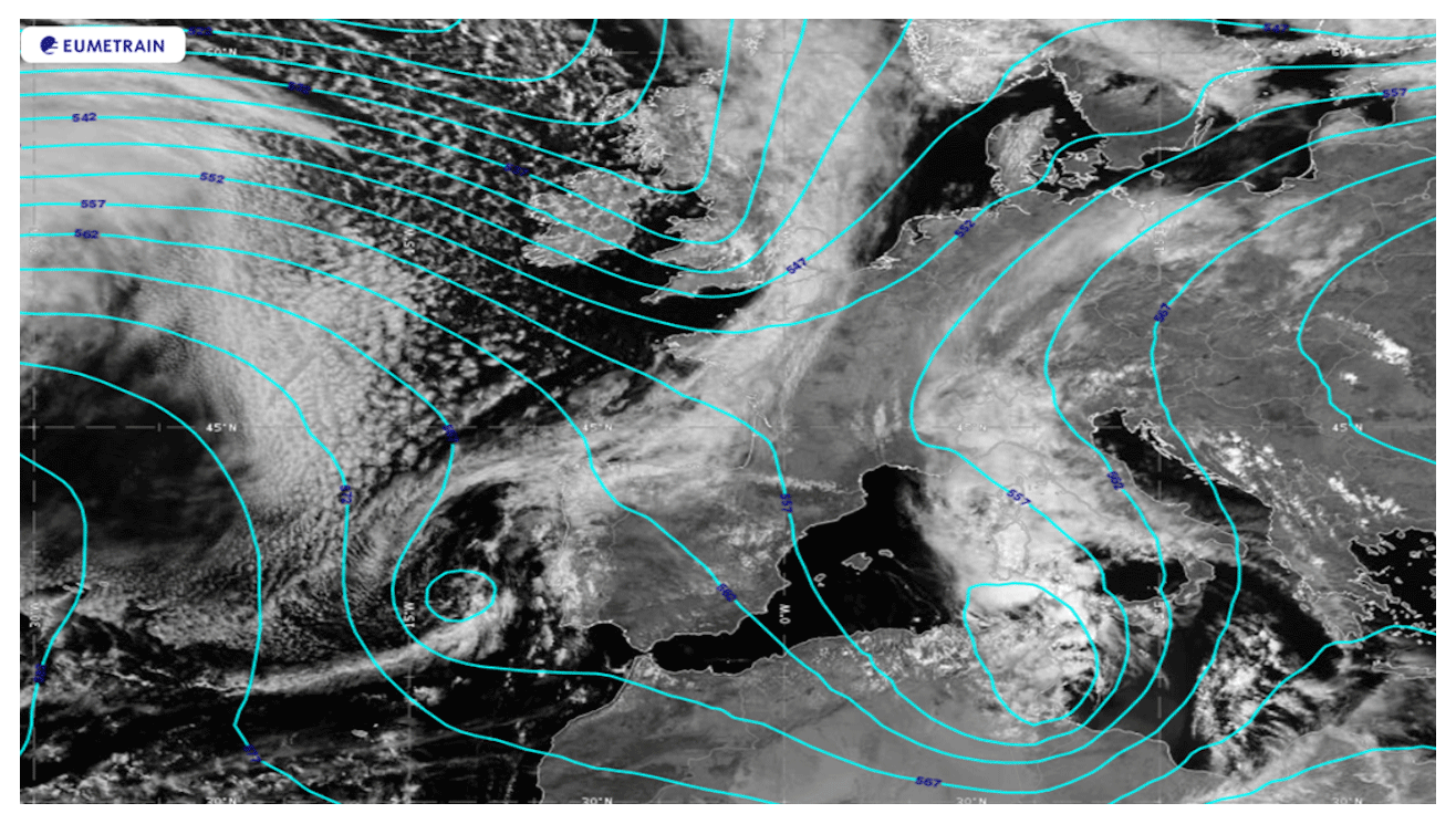
Figure 1 ECMWF analysis: geopotential height at 500 hPa (cyan lines, contour lines 5 dam) and visible satellite image on 2 May 2018 at 12:00 UTC. Image retrieved from Eport portal – EUMeTrain.

This study aims to (i) assess the performance of 1 h cycling assimilation with 3D-Var and 4D-Var methods using the WRF model; (ii) evaluate the impact of the radar reflectivity mosaic, acquired by the Italian radar network, in cycling assimilation with variational methods; and (iii) quantify the improvements of assimilation techniques in terms of QPF for a complex orography region in the Mediterranean basin. In this regard, a heavy rain case that occurred in central Italy on 3 May 2018 is used and several experiments are carried out to quantify the impact of the two assimilation methods in cycling mode. With the aim of identifying the best configuration in terms of QPF, two different statistical methods are applied: a filtering (neighbourhood) technique and a receiver operating characteristic (ROC) statistical indicator. The key novelties of this paper are (i) the application of hourly cycling 4D-Var assimilation with the WRF model, (ii) the comparison between the two variational assimilation methods 3D/4D-Var in cycling mode, and (iii) the assessment of the precipitation forecast skill of cycling 3D/4D-Var assimilation methods in an orographically complex region.

The paper is organized as follows. The case study is described in Sect. 2, while the assimilated dataset is presented in Sect. 3. Section 4 contains a brief overview of the assimilation and verification methods, while the model's setup and experiment design are described in Sect. 5. The results are summarized in Sect. 6. Lastly, the conclusions are discussed in Sect. 7.

2 Case study

On 2 May 2018, the synoptic scenario was characterized by an upper level trough at tear-off stage extended from central Europe to northern Africa whose evolution was slowed by the presence of two anticyclonic circulations over the Atlantic Ocean and Russia (Fig. 1). The upper level trough, with a northwest–southeast oriented axis, brought cool and dry air from the Arctic region towards the Mediterranean basin and advected a moist and warm south-easterly flow over the Adriatic region. In the following 24 h, the upper level trough evolved in a cut-off low, producing a surface low-pressure system (992 hPa) on the western side of Sicily (Fig. 2a). The surface depression slowly moved north-eastward, dissipating its energy over the next 12 h.

The mesoscale conditions over Italian peninsula showed a strong and moist south-easterly flow at the upper and middle atmospheric levels, whereas a convergency line between the north-eastern (Bora) and south-eastern (Sirocco) winds developed at low levels (Fig. 2b). This produced heavy precipitation on 3 May over the central Italy Adriatic region, which was enhanced by the complex orography of this area. Indeed, the highest peaks of the Apennines mountains (Gran Sasso and Majella at 2912 m and 2793 m a.m.s.l., respectively) near the coast further increased the atmospheric instability, promoting the triggering of convective cells.

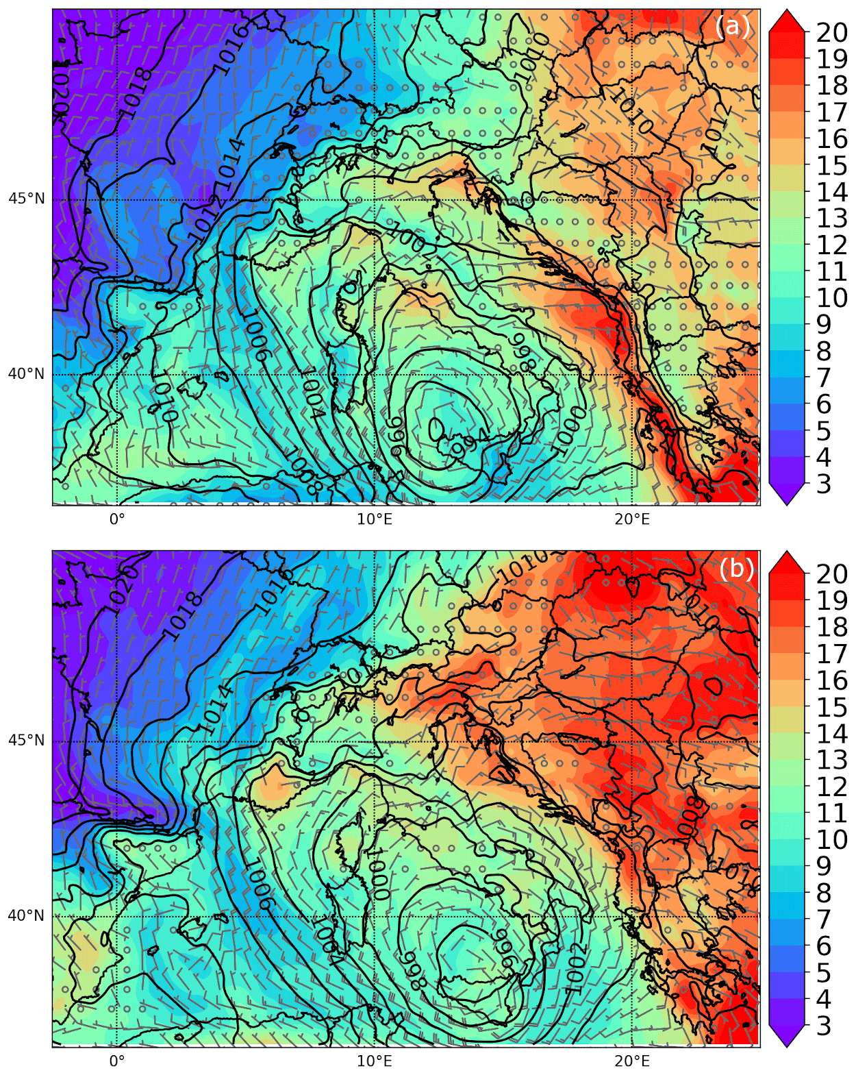
Figure 2 ECMWF analyses: 850 hPa temperature (^∘C), wind field (wind barbs) at 950 hPa and sea level pressure (black lines) on 3 May at 6:00 UTC (a) and 12:00 UTC (b).

Relevant daily accumulations were reported in the Gran Sasso mountainous area with values ranging from 80 and 90 mm, except the rain gauge station located in Fano a Corno, which measured 152 mm. The precipitation also affected the coastal sector with amounts of 73 mm at Pescara and Pineto and 42 mm at Vasto (Fig. 3).

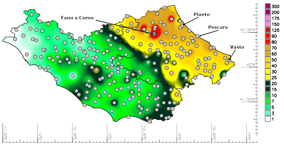
Figure 3 Observed daily precipitation (mm) on 3 May 2018 in the Lazio Abruzzo regions. The points represent the locations of rain gauges. Data courtesy of Italian Civil Protection Department.

3 Datasets description

Related to the aim of assessing the impact of cycling 3D-Var and 4D-Var, the composite radar reflectivity provided by the Italian radar network (Vulpiani et al., 2008) are assimilated in WRF for the numerical simulations.

The Italian ground radar network includes 20 C-band and 3 X-band radar, managed by 11 regional administrations. Among these, 7 C-band and the 3 X-band systems (all with dual-polarization capability) are managed directly by the Italian Civil Protection Department (DPC), which is also the developer and distributor of the national precipitation product. The processing architecture is basically composed of two main steps: firstly, the radar measurements are locally processed by a unique software system and, secondly, all products are centralized to generate the national level products.

Different sources of error can affect the radar measurements (Collier, 1996): non-weather returns (clutter), partial beam blocking, beam broadening at increasing distances, vertical variability of precipitation, radio local area network (RLAN) interference and rain path attenuation. Due to the morphology of the Italian territory, the uncertainty can be mainly associated with the orography-related effects, especially in southern Italy where the radar coverage as well as the radar overlapping is poor.

The DPC processing system aims at identifying most of the uncertainty sources in order to compensate for them, whenever possible, before estimating precipitation. A point-by-point description of the operational radar processing chain can be found in Petracca et al. (2018). After processing, some composite products are generated in real time by DPC and disseminated at the national and regional level. Among these, the reflectivity constant altitude plan position indicator (CAPPI) at 2000, 3000 and 5000 m m.s.l., which covers the whole Italian territory, are assimilated into the WRF model.

It is worth mentioning that the CAPPI gives a horizontal cross section of the data at constant altitude; it is a two-dimensional areal representation extracted from three-dimensional radar volume scan data.

Moreover, a thinning is applied to the CAPPI reflectivity data to ensure uncorrelated observation errors (Chang et al., 2014; Liu and Rabier, 2003) and to reduce the computational complexity, especially for the 4D-Var method. CAPPI data are thinned over the 3 km domain grid (described in Sect. 5.2) using an ad hoc procedure. The rainfall data to assess the impact of 3D/4D-Var methods in cycling mode are provided by the rain-gauge network of the DPC composed of roughly 3000 tipping bucket gauges with a minimum detectable rain amount of 0.2 mm. A careful quality check is applied to the data before using them in the statistical analysis (Hanachi et al., 2014). More specifically, the following actions are performed:

• control of rain gauges with the same name but different coordinates

• removal of data associated with rain gauges without valid coordinates

• removal of duplicate data

• identification of anomalous data (for example very different values with respect to the surrounding rain gauges).

4 Variational data assimilation

The WRF model (Skamarock et al., 2019) is used for the numerical simulations, while the CAPPI radar data are assimilated using the WRF data assimilation system (WRFDA; Barker et al., 2012). This system contains the algorithms required by 3D/4D-Var variational assimilation methods that are described in the following subsections. In this study, 4D-Var is employed in cycling mode to reduce the computational cost and compared with the widely used 3D-Var, again with a cycling update.

4.1 3D-Var and 4D-Var methods

Currently, the WRF 3D-Var (Barker et al., 2012) variational assimilation method is widely applied in meteorological and oceanographic modelling to assimilate a large variety of observations and to generate reliable initial conditions. The 3D-Var is a mathematical technique that combines observations and a short-range forecast (first guess) through the minimization of a cost function. The goal of this method is to reduce the misfit between the observation and the background fields to obtain the best estimate of the true state of the atmosphere. In general, the cost function with respect to an atmospheric state vector x is defined as follows:

$$\begin{array}{}\text{(1)}& \begin{array}{rl}J\left(\mathit{x}\right)=& {\displaystyle \frac{\mathrm{1}}{\mathrm{2}}}\left\{{\left(\mathit{x}-{\mathit{x}}_{\mathrm{b}}\right)}^T{\mathbf{B}}^{-\mathrm{1}}\left(\mathit{x}-{\mathit{x}}_{\mathrm{b}}\right)+{\left[y_{\mathrm{0}}-\mathbf{H}\left(\mathit{x}\right)\right]}^T\right.\\ & \left.{\mathbf{R}}^{-\mathrm{1}}\left[y_{\mathrm{0}}-\mathbf{H}\left(\mathit{x}\right)\right]\right\},\end{array}\end{array}$$

where B and R are the background and observation error matrices, respectively; y₀ represents the observations vector, x_b the background field or first guess and finally H is the forward observation operator that converts data from the model space to observation space.

The 3D-Var method has the advantage of being computationally cheap even if it misses the time dependency; hence, all the observations that are acquired during the assimilation window are considered at its central time.

The WRF 4D-Var (Huang et al., 2009) takes the time variable into account using a numerical weather forecast as dynamical constraint. More specifically, the method computes the model trajectory that reduces the misfit with the observations distributed in the assimilation window. The initial atmospheric state is determined by minimizing the following cost function (Eq. 2):

$$\begin{array}{}\text{(2)}& \begin{array}{rl}J\left({\mathit{x}}_{\mathrm{0}}\right)& ={\displaystyle \frac{\mathrm{1}}{\mathrm{2}}}{\left({\mathit{x}}_{\mathrm{0}}-{\mathit{x}}_{\mathrm{0}}^{\mathrm{b}}\right)}^T{\mathbf{B}}^{-\mathrm{1}}\left({\mathit{x}}_{\mathrm{0}}-{\mathit{x}}_{\mathrm{0}}^{\mathrm{b}}\right)\\ & +{\displaystyle \frac{\mathrm{1}}{\mathrm{2}}}\sum _{k=\mathrm{0}}^n{\left\{y_{\mathrm{0}}^k-H_k\left[M_k\left({\mathit{x}}_{\mathrm{0}}\right)\right]\right\}}^T\\ & {\mathbf{R}}^{-\mathrm{1}}\left\{y_{\mathrm{0}}^k-H_k\left[M_k\left({\mathit{x}}_{\mathrm{0}}\right)\right]\right\}.\end{array}\end{array}$$

The assimilation window is divided into k discrete sub windows, where x₀ is the analysis state vector at time k₀ and H_k and M_k are the nonlinear forward and observation models, respectively. Finally, B and R are, as already mentioned, the background and observation error matrices.

The 4D-Var has the advantage of assimilating the observation at its exact time compared to 3D-Var, ensuring a more consistent physics and dynamical balance of the initial conditions. Given the high computational complexity, the incremental approach proposed by Courtier et al. (1994) has been adopted. The tangent linear and adjoint model with a simplified physics is used in the inner loop to increase the computational efficiency. Despite that the application of 4D-Var in operational mode, it is still limited to the major weather centres only. The B matrix is a key component in the assimilation processes because it weights the errors in the background field adjusting the spatial spreading of observational information. In this context, the National Meteorological Center (NMC) method (Parrish and Derber, 1992), widely use in the data assimilation community, has been adopted for this work. The B matrix is estimated by evaluating the difference between forecasts valid at the same time, but one of them is initialized 12 h after the other. In more detail, the new method (Wang et al., 2013b) considers u, v, temperature, pseudo-relative humidity and surface pressure as control variables, in contrast with the old method, which utilizes the stream function, the unbalanced velocity potential and the unbalanced temperature. Recent studies using the new method, show a slight benefit in the precipitation forecast skill as well as a performance improvement when radar data are assimilated (Wang et al., 2013a, c; Sun et al., 2016). Thus, for this work, the B matrix is computed over a period of 2 weeks from 1 to 15 May 2018 using this new method. According to the values provided in Mazzarella et al. (2020), the var_scaling, and len_scaling parameters adjust the influence of the B matrix over the background field. Len_scaling controls the spatial decorrelation for the following five variables: unbalanced velocity potential, unbalanced temperature, pseudo-relative humidity, unbalanced surface pressure and stream function. The use of a len_scaling factor of 0.5 reduces the variable perturbation length scale by 50 %, ensuring that the water vapour increments are comparable with the weather radar range; therefore, this value has been adopted for the simulations.

The no-echo option, developed by Min and Kim (2016), allows the assimilation of null-echo within the radar observation range. This information reduces the excessive humidity and the contents of the following hydrometeors: snow, graupel and rainwater based on radar reflectivity, improving the convective precipitation predictability. In addition, a recent study (Lee et al., 2020) confirms the benefit of this option for the simulation of three summer convective events over the Seoul metropolitan area. For this reason, the no-echo option is used for this study.

4.2 Radar observation operator

The assimilation of CAPPI radar reflectivity for both 3D/4D-Var assimilation methods was performed through the indirect method (Wang et al., 2013a; Gao and Stensrud, 2012). The new approach converts the observed reflectivity in the three hydrometeor mixing ratios in contrast to the direct method (Xiao and Sun, 2007), which only uses the rainwater mixing ratio.

The forward reflectivity operator considers the contribution of snow, rain and hail components and it is represented as

$$\begin{array}{}\text{(3)}& Z_{\mathrm{e}}\left\{\begin{array}{ll}Z\left(q_{\mathrm{r}}\right),& T_{\mathrm{b}}>\mathrm{5}{}^{\circ }\mathrm{C}\\ Z\left(q_{\mathrm{s}}\right)+Z\left(q_{\mathrm{h}}\right),& T_{\mathrm{b}}<-\mathrm{5}{}^{\circ }\mathrm{C}\\ aZ\left(q_{\mathrm{r}}\right)+(\mathrm{1}-a)\left[Z\left(q_{\mathrm{s}}\right)+Z\left(q_{\mathrm{h}}\right)\right],& -\mathrm{5}{}^{\circ }C<T_{\mathrm{b}}<\mathrm{5}{}^{\circ }\mathrm{C}\end{array}\right.\end{array}$$

where Z_e is the equivalent reflectivity factor, a varies linearly between 0 at $T_{\mathrm{b}}=-\mathrm{5}$ ^∘C and 1 at T_b=5 ^∘C, and T_b is the background temperature from an NWP.

The three hydrometeor mixing ratios, rain (q_r), snow (q_s) and hail (q_h) in Eq. (3) are calculated using the formulation proposed by Lin et al. (1983), Gilmore et al. (2004) and Dowell et al. (2011).

The rain contribution to the equivalent reflectivity (Smith et al., 1975) is calculated as follows:

$$\begin{array}{}\text{(4)}& Z\left(q_{\mathrm{r}}\right)=\mathrm{3.63}\times {\mathrm{10}}^{\mathrm{9}}{\left(\mathit{\rho }{q}_{\mathrm{r}}\right)}^{\mathrm{1.75}},\end{array}$$

where ρ is the air density.

The snow component is divided into dry and wet snow according to the T_b temperature:

$$\begin{array}{}\text{(5)}& {\displaystyle }& {\displaystyle }Z\left(q_{\mathrm{s}}\right)=\mathrm{9.80}\times {\mathrm{10}}^{\mathrm{8}}{\left(\mathit{\rho }{q}_{\mathrm{s}}\right)}^{\mathrm{1.75}},\mathrm{if}{T}_{\mathrm{b}}<\mathrm{0}{}^{\circ }\mathrm{C}\text{(6)}& {\displaystyle }& {\displaystyle }Z\left(q_{\mathrm{s}}\right)=\mathrm{4.26}\times {\mathrm{10}}^{\mathrm{11}}{\left(\mathit{\rho }{q}_{\mathrm{s}}\right)}^{\mathrm{1.75}},\mathrm{if}{T}_{\mathrm{b}}\mathrm{is}>\mathrm{0}{}^{\circ }\mathrm{C}.\end{array}$$

For the hail component, the formulation based on Lin et al. (1983) and Gilmore et al. (2004) is adopted:

$$\begin{array}{}\text{(7)}& Z\left(q_{\mathrm{h}}\right)=\mathrm{4.33}\times {\mathrm{10}}^{\mathrm{10}}{\left(\mathit{\rho }{q}_{\mathrm{h}}\right)}^{\mathrm{1.75}}.\end{array}$$

Some microphysics schemes do not produce hail component, but WRFDA code recognizes them and uses the q_h variable as a graupel species q_g (Lagasio et al., 2019).

Finally, the equivalent reflectivity (Z_e), given by the sum of the three components Z(q_s), Z(q_r) and Z(q_h), is converted into Z (dBZ) using

$$\begin{array}{}\text{(8)}& Z_{\mathrm{dB}}=\mathrm{10}{\log }_{\mathrm{10}}{Z}_{\mathrm{e}}.\end{array}$$

The option allowing the assimilation of in-cloud humidity from radar reflectivity was considered for this study (Wang et al., 2013a). The estimate of the saturated water vapour observation is produced considering the assumption that in-cloud humidity is saturated. The in-cloud relative humidity is assumed to be 100 % where radar reflectivity is higher than a threshold above cloud base, so that the estimated water vapour equals to the saturation water vapour that is calculated in Eq. (9) based on the pressure and temperature of the background. In this paper, the threshold is set to 25 dBZ (WRFDA default value). A full description of the indirect assimilation method is provided in Wang et al. (2013a). The forward observed operator H is defined by

$$\begin{array}{}\text{(9)}& q_{\mathrm{v}}=\mathrm{RH}\times q_{\mathrm{sh}},\end{array}$$

where q_v represents the specific humidity, RH the relative humidity and q_sh the saturated specific humidity of water vapour. It is worth noticing that the assimilation of the in-cloud humidity is used in combination with indirect assimilation. Thus, the numerical experiments also include the assimilation of in-cloud humidity in addition to the hydrometeor species retrieved with the indirect method alone.

5 Model setup

The numerical simulations are carried out with the ARW-WRFV4.0 model (Skamarock et al., 2019). WRF is a mesoscale model, supported by National Center for Atmospheric Research (NCAR) and largely used by the atmospheric modelling community. The main features consist of fully compressible Euler nonhydrostatic equations with a hydrostatic option, staggered Arakawa C grid, and highly portable and flexible code that optimizes the use of computational resources.

A two-way nesting configuration with two domains is used for this study: the mother domain with 379×431 grid points, covers the Italian peninsula with a horizontal resolution of 3 km, while the inner domain (340×319 grid points) is centred over the Abruzzo region (central Italy) with a grid spacing of 1 km (Fig. 4a). To avoid compatibility issues with WRFDA, the vertical terrain-following coordinates are used instead of the terrain-following hybrid. Both domains adopt 40 vertical levels from the ground up to 100 hPa. Because of the high spatial resolution, the convection is explicitly resolved. The same physical parameterizations used by the Center of Excellence in Telesensing of Environment and Model Prediction of Severe Events (CETEMPS) meteorological–hydrological forecast system are used for this work (Ferretti et al., 2014). More specifically, the microphysical processes are parameterized using the WSM6 scheme (Hong and Lim, 2006), while the Mellor–Yamada–Janjic (MYJ) scheme (Janjić, 1994) is applied for the planetary boundary layer (PBL). Shortwave and longwave radiation are considered through the rapid radiative transfer model (RRTM) scheme (Mlawer et al., 1997). Finally, the Noah land surface model is chosen to parametrize the land surface processes (Chen and Dudhia, 2001). The operational analysis and forecast cycles from the integrated forecast system (IFS) global model of the European Centre for Medium-Range Weather Forecasts (ECMWF) with a spatial resolution of $\mathrm{0.1}{}^{\circ }\times \mathrm{0.1}{}^{\circ }$ are used for this work and the boundary conditions are updated every 3 h.

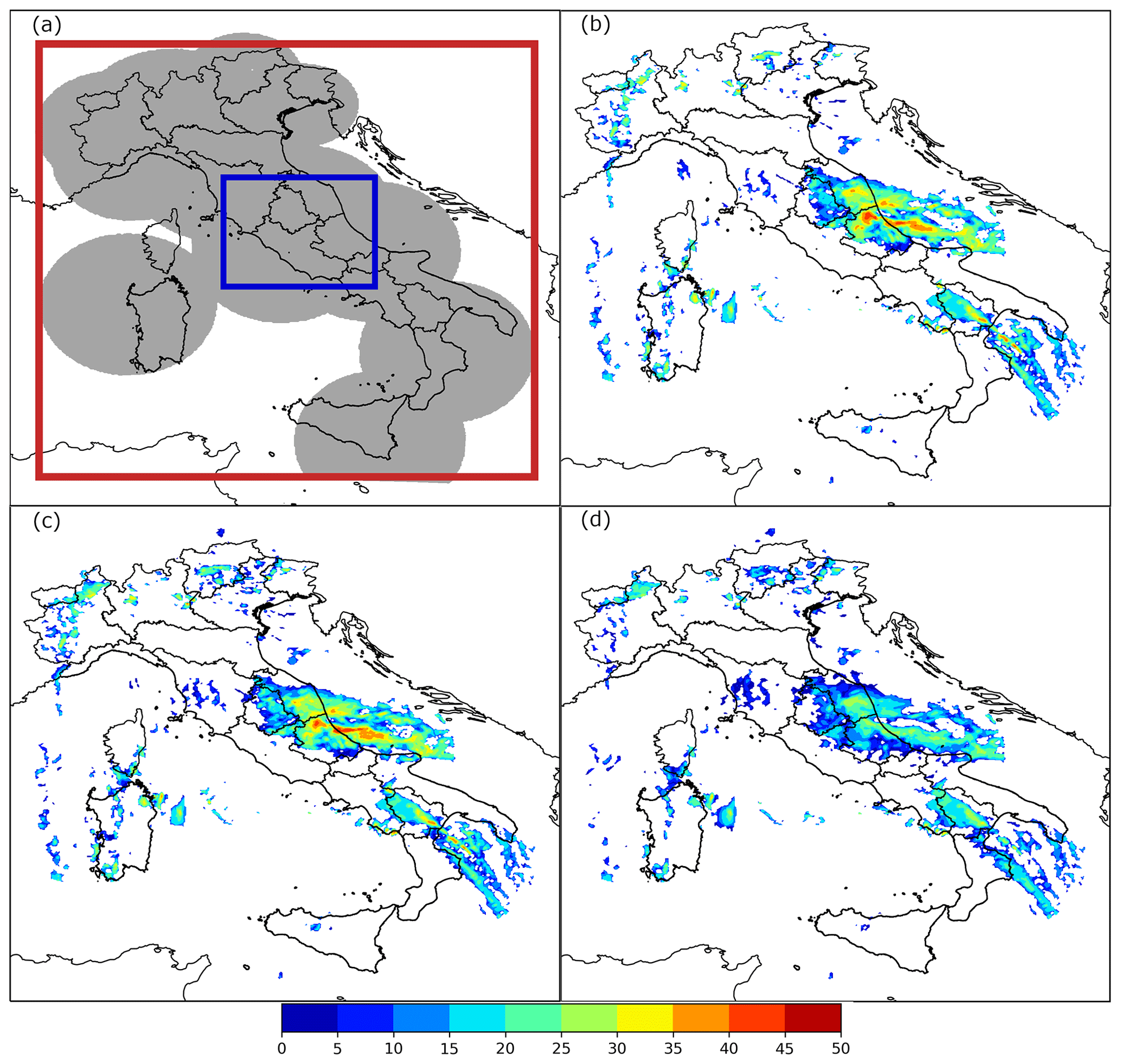
Figure 4 Spatial coverage of the Italian radar network (grey area). The two rectangles represent the WRF domains: 3 km (in red) and 1 km (in blue) (a). Three examples of CAPPI radar reflectivity (dBZ) at 2 km (b), 3 km (c) and 5 km (d) assimilated at 02:00 UTC on 3 May 2018.

5.1 Design of experiments

A total of five experiments are carried out to evaluate the impact of 3D/4D-Var in cycling mode. All simulations started at 00:00 UTC on 3 May 2018 and lasted for 24 h. Both 3D-Var and 4D-Var are applied every hour in cycling mode from 00:00 to 03:00 UTC assimilating the CAPPI reflectivity data at 2000, 3000 and 5000 m MSL. The same number of observations was assimilated for both 3D-Var and 4D-Var simulations, considering a 10 min assimilation window. More specifically, the CAPPI are assimilated at 00:00, 00:10, 01:00, 01:10, 02:00, 02:10, 03:00 and 03:10 UTC (Fig. 4b–d). Moreover, two additional simulations are performed with the aim of evaluating the performance of cycling assimilation methods in warm start mode. For this purpose, a previously numerical forecast, initialized 6 h before, is used as background field. The same aforementioned CAPPI are assimilated in these experiments.

Table 1 summarizes the experiments performed.

Table 1 Description of the five simulations performed.

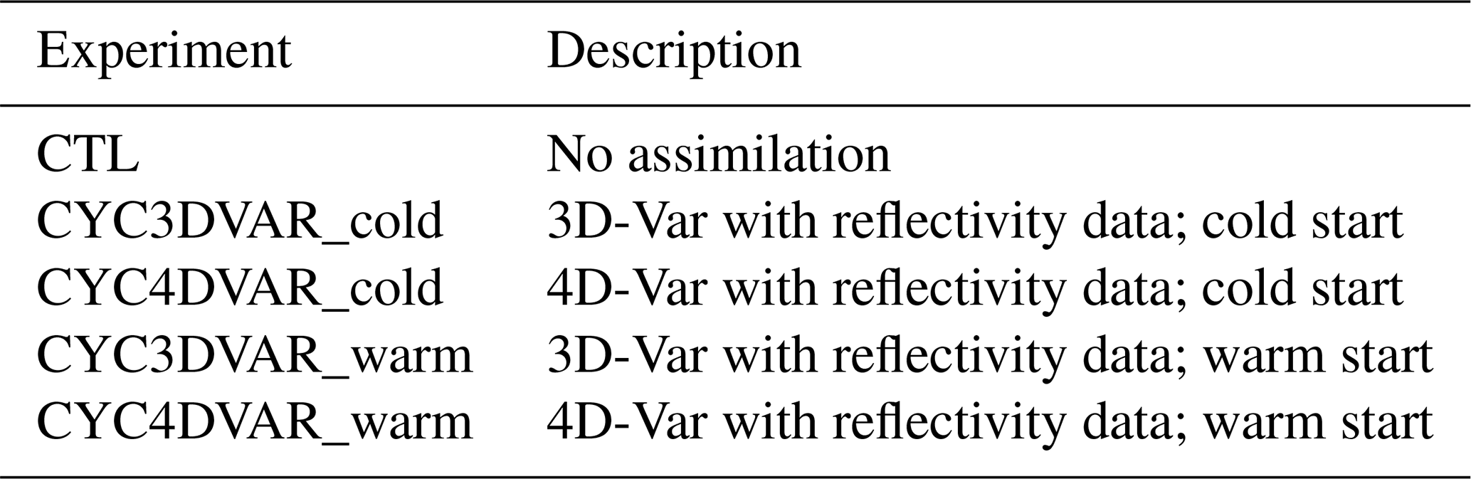
Figure 5 Rainwater mixing ratio (kg kg⁻¹) analysis increments at vertical level 15 from the CYC4DVAR_warm (a), CYC3DVAR_warm (b), CYC4DVAR_cold (c) and CYC3DVAR_cold (d) experiments.

5.2 Verification methodologies

Related to the aim of evaluating the impact of both 3D-Var and 4D-Var in cycling mode, an objective comparison between the observed and forecast precipitation is performed. For this purpose, the rainfall data collected by the DPC rain gauge network are spatially interpolated on the model grid. In more detail, the inverse distance weighting (IDW) conservative method (Jones, 1999) is used to re-map the rain data to the 3 km domain grid. The statistical analysis is only performed in a restricted area of the mother domain (Fig. 4a, red rectangle) that includes the Lazio and Abruzzo regions (hereafter LA; Fig. 3), because these are the regions where relevant accumulated precipitations was recorded.

Finally, this work represents a preliminary study to investigate the reliability of the cycling assimilation before implementing it in an operational meteorological–hydrological chain like the operative at CETEMPS, which focused on the meteorological–hydrological forecast in the Abruzzo region.

To avoid the spatial limitations of using a point-by-point approach in the evaluation of quantitative precipitation forecast (Roberts, 2003), a filtering method is used. Based on the positive response in the recent literature (Tong et al., 2016; Wang et al., 2013c; Romine et al., 2013; Gustafsson et al., 2018), the fraction skill scores (FSS; Roberts and Lean, 2008) are computed for the precipitation assessment. A few accumulated periods are considered related to the aim of investigating the forecast ability for different kinds of precipitation. For the 3-hourly accumulated precipitation, a neighbourhood size of 3x3 grid points is used for this purpose.

In addition, the receiver operating characteristic (ROC) statistical indicator is computed to strengthen the statistical analysis, evaluating how skilful the cycling assimilation methods are in terms of QPF. The ROC curve synthesizes the information obtained with different thresholds in one diagram, just comparing the hit rate against false alarm rate (Swets, 1973). Finally, the area under the ROC curve (AUC), which is largely used to quantify the skill of a forecast system (Mason, 1982; Buizza and Palmer, 1998; Storer et al., 2019; Ferretti et al., 2020), is calculated for each simulation.

Before presenting the results related to the aim of clarifying the impact of reflectivity CAPPI at 2, 3 and 5 km in cycling 3D/4D-Var methods, the analysis increments (analysis minus first guess) are calculated at the end of the last assimilation cycle (03:00 UTC). The assimilation of radar reflectivity mainly impacts water vapour and cloud hydrometeors variables, rather than temperature and wind components. Therefore, the analysis increments for q_r (rainwater mixing ratio; Fig. 5) and q_v (water vapour mixing ratio; not shown), which best represent the added value of the radar reflectivity assimilation, are considered. For this purpose, vertical level 15 (about 2000 m above ground) is selected because the influence of radar data is more relevant. A qualitative comparison between the two assimilation methods points out that the 4D-Var is more impactful in terms of q_r both with a warm (Fig. 5a) and cold start (Fig. 5c) compared to 3D-Var (Fig. 5b and d). Furthermore, the larger analysis increments of q_r are along the Adriatic Sea near the Abruzzo coastline in agreement with the assimilated CAPPI maps, which show high reflectivity values in this area. The distribution of the analysis increments for the q_v (not shown here) is similar to the previous analysis increments (q_r in Fig. 5), but the magnitude becomes larger than q_r. The 4D-Var simulations produce greater q_v increments compared to 3D-Var, in line with the next result.

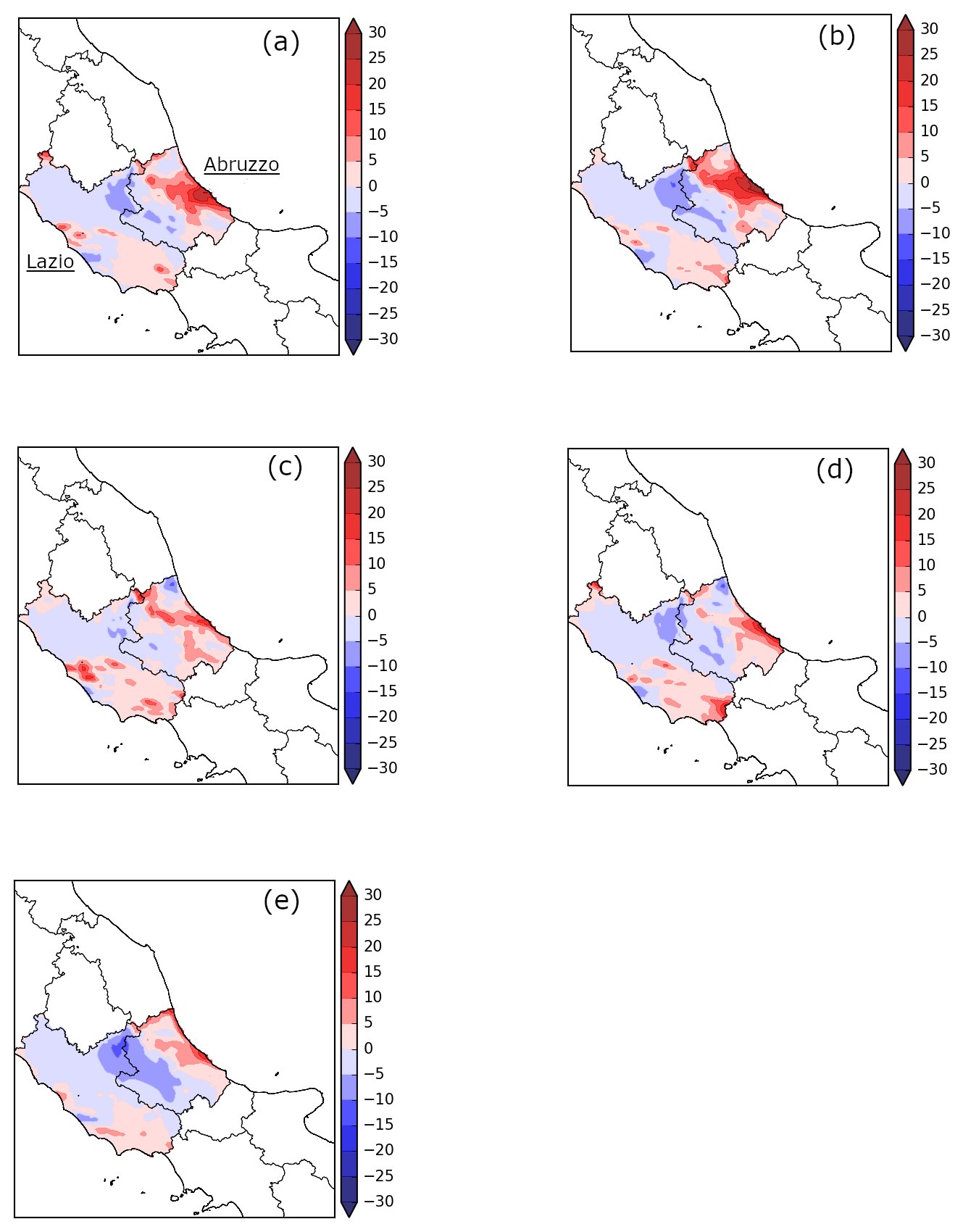
Figure 6 Differences (mm) between observed and predicted 3-hourly precipitation fields for the CYC4DVAR_cold (a), CYC3DVAR_cold (b), CYC4DVAR_warm (c), CYC3DVAR_warm (d) and CTL (e) simulations in the Lazio Abruzzo regions.

6 Results

A preliminary qualitative comparison is performed with the aim of explaining the impact of cycling assimilation in short-term rainfall prediction. For this purpose, the differences between forecast and observed precipitation fields have been calculated for each simulation considering the rainfall amounts from 09:00 to 12:00 UTC when the FSS shows the highest values and the gap between the different simulations is more meaningful.

The results (Fig. 6) confirm the positive impact of cycling assimilation: both methods reduce the underestimation of the rainfall (blue area) over the mountain area at the border between the Lazio and Abruzzo regions. In this context, the 4D-Var and 3D-Var experiments with a warm start initialization show the best performances in this area (Fig. 6c and d), improving the precipitation forecast accuracy compared to the control experiment (CTL) (Fig. 6e). Conversely, the two simulations in cold mode overestimate the rainfall along the coastal area of the Abruzzo region even though they partially mitigate the error in the internal areas (Fig. 6a and b).

6.1 Statistical evaluation

Related to the aim of evaluating the performance of 3D-Var and 4D-Var assimilation methods in cycling mode, the FSS and ROC, previously described in Sect. 5.2, were calculated. The FSS is calculated in the LA region, where significant precipitation occurred. To this purpose, several threshold values are used to evaluate the impact of cycling assimilation with light, moderate and heavy precipitation. Finally, the ROC and AUC are calculated to reinforce the statistical analysis and summarize the information obtained with the FSS.

To compare the 3D/4D-Var experiments in a warm/cold start and their ability to reproduce the precipitation pattern, the statistical index was calculated considering the precipitation accumulated over three specified time periods: 1, 3 and 6 h, respectively. The time series of FSS is presented in the sections below.

6.1.1 Hourly precipitation

The FSS for the 1 mm h⁻¹ accumulated threshold (Fig. 7a) is calculated for all the experiments starting from 06:00 to 15:00 UTC in the LA region. The results are quite similar for all experiments in the first hour of simulation due to the small amount of accumulated precipitation, even though CTL starts from higher values than the other experiments. Later, all experiments display higher FSS values than the CTL experiment (red dashed line), pointing out the positive feedback of cycling assimilation in the interval from 07:00 to 12:00 UTC. Moreover, the simulations with warm initialization clearly show (Fig. 7a, blue and green lines) higher values, demonstrating a larger impact on the precipitation forecast than those with a cold start. On the other hand, CTL performs better in the last 3 h of simulation, suggesting that the positive impact of radar reflectivity assimilation decreases with time. The FSS computed for the 3 mm h⁻¹ threshold (moderate precipitation) is shown in Fig. 7b. The simulations with data assimilation confirm the improvements in terms of QPF from 07:00 to 12:00 UTC. In addition, the two experiments with 4D-Var (Fig. 7b, yellow and blue lines) performs better than 3D-Var, except in the first hours of the simulation. This behaviour proves the positive impact of 4D-Var with moderate precipitation. However, similarly to the results for the 1 mm h⁻¹ threshold, the impact of radar reflectivity assimilation decreases towards the end of the simulation. Finally, the FSS is calculated for the 8 mm h⁻¹ threshold (Fig. 7c) in conformity with World Meteorological Organization (WMO, 2003), which classifies the precipitation with a rain rate greater than 7.6 mm h⁻¹ as heavy rain. According to the results for the 3 mm h⁻¹ threshold, the FSS confirms the good performance of 4D-Var in cycling mode. More specifically the CYC4DVAR_warm (Fig. 7c, blue line) shows the highest FSS values in the whole period with heavy precipitation, except for a very short period where the 4D-Var cold start reaches higher values than the warm start. Conversely, the benefit of 3D-Var simulations is limited to the first hours of the simulation.

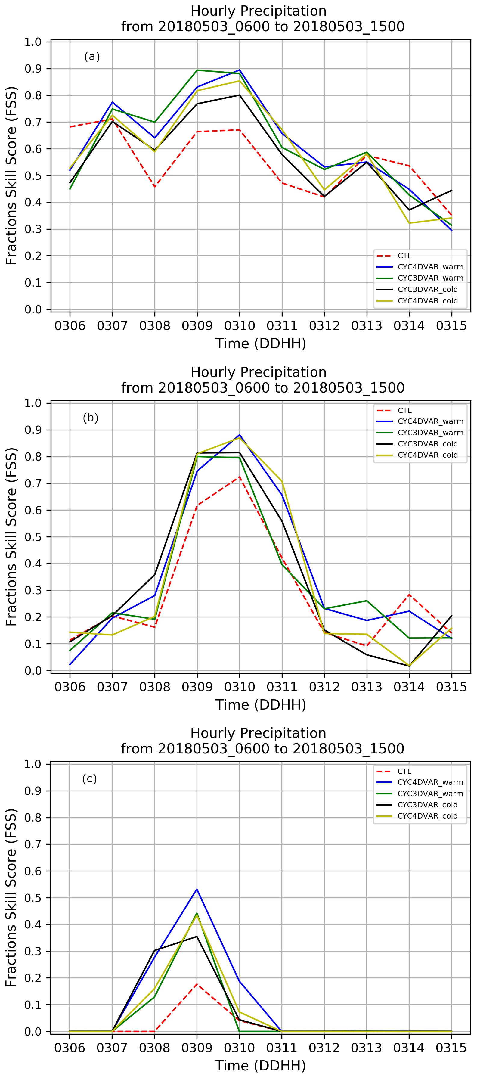
Figure 7 Evolution of FSS calculated in the LA region considering the hourly accumulated precipitation for three threshold values: 1 mm h⁻¹ (a), 3 mm h⁻¹ (b) and 8 mm h⁻¹ (c). The dashed red line represents the CTL, the blue line CYC4DVAR_warm, the green line CYC3DVAR_warm, the black line CYC3DVAR_cold, and the yellow line CYC4DVAR_cold.

The statistical analysis with hourly precipitation clearly shows the positive impact of assimilation in the cycling mode with both methods in the initial hours of the simulation. Moreover, the simulations in warm mode show the best performance compared to those with a cold start, especially the CYC4DVAR_warm (Fig. 7c, blue line) when heavy precipitation occurred.

6.1.2 Three-hourly precipitation

The statistical analysis is also carried out for the 3-hourly precipitation accumulation interval to deeper investigate the response of cycling data assimilation for precipitation characterized by different mechanisms, for example convection or orographic uplifting. The FSS for the 1 mm 3 h⁻¹ threshold (Fig. 8a) highlights the benefit of using 3D and 4D-Var with a cold start for a short initial period (06:00–07:30 UTC), suggesting that the background field is probably more accurate than the previous forecast. But the rate of increasing for both of the warm starts is larger than the CTL and cold starts. Indeed, the FSS values for the warm start are higher than the cold starts up to 12:00 UTC (Fig. 8a, blue and green lines). Later, the improvement reduces, and CTL performs better (Fig. 8a, red dashed line). The score is also computed for the 3 mm 3 h⁻¹ threshold (Fig. 8b). Similarly to the results for the 1 mm threshold, the cycling 4D-Var in cold mode (CYC4DVAR_cold) improves the precipitation forecast at the initial time (06:00 to 08:00 UTC), while the CYC4DVAR_warm mode confirms the highest values from 09:00 to 12:00 UTC as well as the poor performance in the first hour. Moreover, the reduction in FSS values for both 4D-Var and 3D-Var compared to CTL in the final hours of simulation period proves that the influence of cycling is restricted to a short time range.

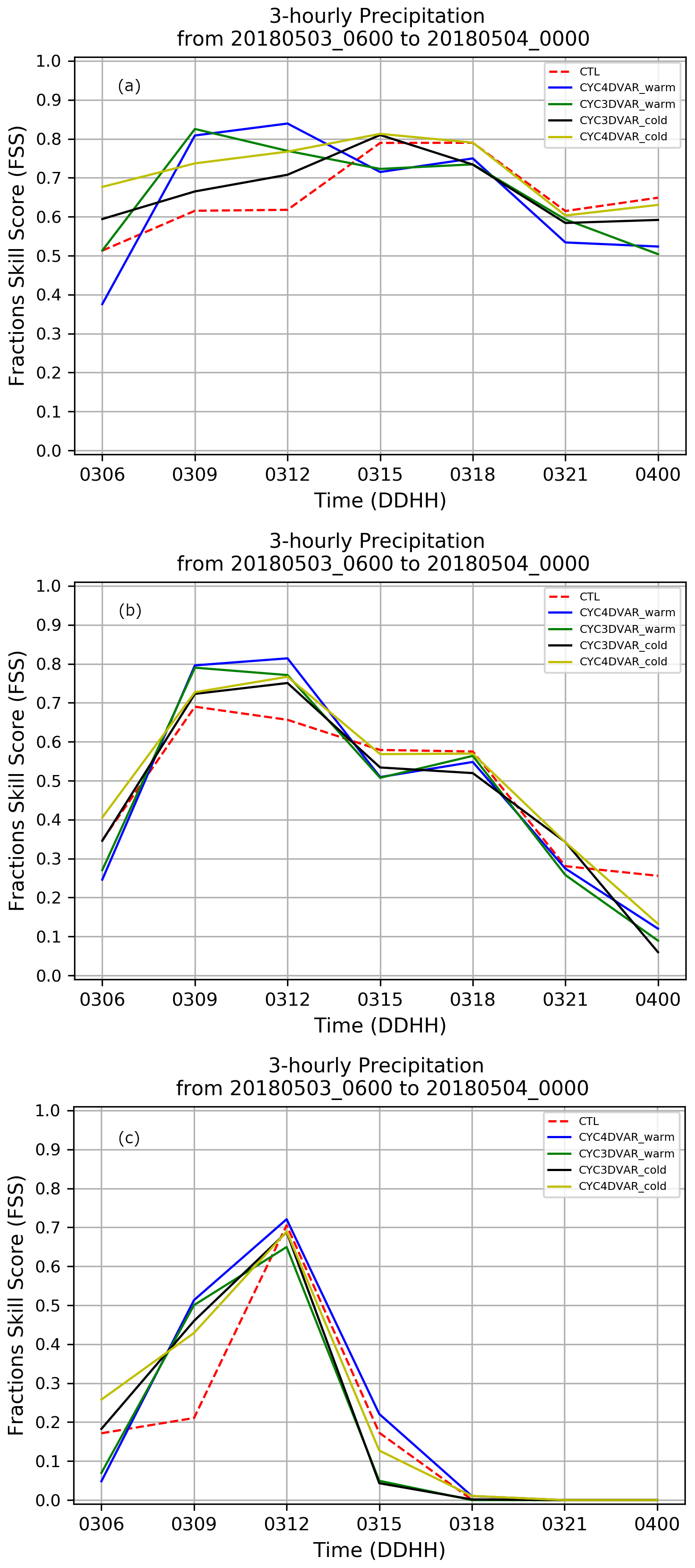
Figure 8 Evolution of FSS calculated in the LA region considering the 3-hourly accumulated precipitation for three threshold values: 1 mm 3 h⁻¹ (a), 3 mm 3 h⁻¹ (b) and 10 mm 3 h⁻¹ (c). The dashed red line represents the CTL, the blue line CYC4DVAR_warm, the green line CYC3DVAR_warm, the black line the CYC3DVAR_cold and the yellow line CYC4DVAR_cold.

Finally, the FSS is also calculated for the threshold value of 10 mm 3 h⁻¹ in the LA region (Fig. 8c). The highest values are associated with CYC4DVAR_warm (blue line), although all experiments show an improvement compared to the CTL in the first hours of the simulation period. Later, all the experiments converge to the CTL, but the values for FSS decrease due to the small accumulated rainfall.

The statistical analysis performed using the three threshold values (1, 3 and 10 mm) proves the positive impact of cycling assimilation with radar reflectivity in the interval 06:00–15:00 UTC and confirms the benefit of 4D-Var compared to 3D-Var. Moreover, the two simulations with a warm start initialization show a low impact at 06:00 UTC. The reason for this is probably the accuracy of the initial conditions, which is lower than that for the cold start simulation even though the ECMWF operational analysis is used to simulate the first 6 h for the warm start simulations.

6.1.3 Six-hourly precipitation

The FSS is also calculated using the 6-hourly precipitation in the LA region using three threshold values: 10, 15 and 25 mm 6 h⁻¹. The FSS calculated for the 10 mm 6 h⁻¹ threshold (Fig. 9a) proves the positive impact of CYC4DVAR_warm (blue line) compared to the 3D-Var and CTL simulations for the whole simulation interval. The results also suggest that the cycling assimilation with warm start performs better than experiments in cold start for both assimilation methods.

Figure 9 Evolution of FSS calculated in the LA region considering the 6-hourly accumulated precipitation for three threshold values: 10 mm 6 h⁻¹ (a), 15 mm 6 h⁻¹ (b) and 25 mm 6 h⁻¹ (c). The dashed red line represents the CTL, the blue line CYC4DVAR_warm, the green line CYC3DVAR_warm, the black line the CYC3DVAR_cold and the yellow line CYC4DVAR_cold.

According to the results for the previous analysis, the CYC4DVAR_warm confirms the best performance in term of FSS for the 15 mm 6 h⁻¹ threshold (Fig. 9b). Both CYC4DVAR_cold and CYC3DVAR_warm display a positive impact in QPF during the whole simulation period. Conversely, the CYC3DVAR_cold shows a worsening at 18:00 UTC when compared to the CTL and other experiments.

The FSS is also calculated for the 25 mm 6 h⁻¹ (Fig. 9c) threshold to investigate the impact of cycling assimilation with larger accumulated precipitation. The CYC4DVAR_warm shows the highest FSS values, pointing out the benefit of 4D-Var in warm start mode in the whole simulation interval compared to the CTL. Nevertheless, the other simulations with cycling assimilation also show a positive impact in the whole interval, even with a slight improvement up to 18:00 UTC. In conclusion, the time series of FSS points out the benefit of using a cycling assimilation for radar reflectivity. The warm start with 3D/4D-Var assimilation methods confirms the improvement in terms of QPF for the following:

• the hourly accumulated precipitation, highlighting the good performance in the localization and timing of the onset of the precipitation and for very light precipitation

• the 3-hourly accumulated precipitation, highlighting the improvements for convective cells and orographic precipitation

• the 6-hourly accumulated precipitation.

On the other hand, the FSS depends on threshold values; thus, a further statistical indicator was calculated related to the aim of endorsing the previous results. Hence, the ROC curve, which summarizes the result obtained with several thresholds in one plot allowing for an easy comparison, is built for this study.

6.2 Receiver operating characteristic (ROC)

The receiver operating characteristic (ROC), which compares the probability of detection (POD) and false alarm rate (FAR), is calculated to evaluate how skilful the simulations are in precipitation forecast. The 12-hourly precipitation accumulated from 06:00 to 18:00 UTC on 3 May 2018 for the NWP experiments and the rain gauge network are used to build the curve (Fig. 10) for the LA region. To investigate the ability of cycling assimilation in predicting rainfall with light, medium and heavy intensity, the following precipitation thresholds are chosen: 1, 12, 24, 36, 48 and 54 mm. The curves show low POD values for the 1 mm threshold and a worsening compared to the CTL. On the other hand, the benefit of cycling assimilation is clearly found with higher threshold values. In fact, the steepness of 3D/4D-Var curves is greater than CTL, suggesting a good forecast skill with moderate and heavy precipitation – namely, from 12 to 48 mm. In this regard, the CYC4DVAR_warm (green line) shows the best performance, while the CYC3DVAR_cold (red line) reduces its impact with high threshold values. In addition, the area under the curve (AUC) is also computed to objectively compare each curve. The AUC for the cycling 4D-Var experiments is 0.91, while the CTL reaches a lower value of 0.88, confirming the positive impact of 4D-Var in cycling mode, which is in line with the previous results. The 3D-Var simulations, instead, show AUC values comparable to the CTL.

Figure 10 The receiver operating characteristic curves (ROC) are computed for the CTL (black), CYC3DVAR_cold (red), CYC3DVAR_warm (blue), CYC4DVAR_cold (magenta) and CYC4DVAR_warm (green). The 12-hourly accumulated precipitation from 06:00 to 18:00 UTC on 3 May 2018 are used to build the curves.

7 Conclusions

In this paper, the impact of cycling 3D-Var and 4D-Var variational assimilation methods on forecasting a heavy precipitation event occurring in an orographically complex region – namely, central Italy – is evaluated. The reflectivity CAPPI obtained by the Italian radar network at 2, 3 and 5 km are assimilated every hour in cycling mode into the WRF model. The comparison of the experiments is performed using a filtering approach, the fraction skill score (FSS), for the Lazio-Abruzzo regions, where relevant rainfall occurred on 3 May 2018. In this regard, the statistical analysis is performed considering 1-, 3- and 6-hourly accumulated precipitation with three different threshold values in order to evaluate the benefit of cycling assimilation with light, moderate and heavy precipitation. Finally, an ROC curve is built to further evaluate the reliability of cycling assimilation in the precipitation forecast.

The FSS time series for the hourly precipitation highlights the positive impact of radar data for both the 3D-Var and 4D-Var assimilation methods compared to the CTL. The benefit of using a cycling assimilation is clearly shown in the results for both light and moderate precipitation. However, the impact reduces in the last hours of the simulation when all experiments converge to the CTL. Conversely, the poor amount of precipitation at the start time, reduces the impact of both assimilation methods at the start time for the 1 mm h⁻¹ threshold. The results for 3 h precipitation for all thresholds confirm the benefits of assimilating reflectivity data. In this regard, the cycling 4D-Var has a greater impact than 3D-Var experiments and consequently higher FSS value. More specifically, the cold start initializations for cycling both 4D-Var and 3D-Var show an improvement in terms of QPF compared to CTL at the beginning of the analysis, while the experiments in warm start perform better after a few hours. This behaviour is probably caused by a slightly unbalanced initial field for the warm start simulations.

For the 6-hourly precipitation, the FSS for the 10 mm 6 h⁻¹ threshold confirms the improvement of warm start simulations compared to the CTL and cold initialization. The CYC4DVAR_warm clearly displays the greatest FSS values at the 15 and 25 mm 6 h⁻¹ thresholds, pointing out the positive impact of radar reflectivity. Also, the 4D-Var in cold start and the 3D-Var with a warm initialization produce an improvement in QPF, although it is smaller than CYC4DVAR_warm. On the other hand, the CYC3DVAR_cold shows a worsening in FSS.

Finally, the ability of cycling assimilation to reproduce the 12 h precipitation field is evaluated using the ROC and the area under the curve (AUC). The curves are calculated considering the period from 06:00 to 18:00 UTC on 3 May 2018 because of the significant rainfall. The comparison between the simulations confirms that cycling 4D-Var in both warm and cold mode is the best technique; indeed, the highest value of AUC = 0.91 is obtained. The CTL shows lower steepness than the cycling 4D-Var and an AUC of 0.88. Finally, the AUC for the two simulations with 3D-Var (0.87 for the warm initialization and 0.89 for the cold) are lower than 4D-Var and comparable with the CTL simulation. Therefore, the impact of 3D-Var over 12 h accumulated precipitation is less clear.

In conclusion, the cycling assimilation with 3D-VAR and 4D-Var methods for this heavy rain event improves the reliability of the precipitation forecast, even if the positive impact reduces in time. Therefore, to further investigate the impact of cycling assimilation with 3D/4D methods and to generalize the achieved results, a larger number of events should be considered.

Moreover, the two simulations with a warm start initialization produce good results in terms of FSS, but the differences are small compared to the cold simulations that perform better at the initial time. This behaviour suggests that the precipitation spinup time decreases in cycling assimilation with cold start, while for warm initialization this is not true. In addition, the cycling 4D-Var with warm start (CYC4DVAR_warm) shows better performance than 3D-Var over all precipitation accumulation intervals considered for this study. Finally, the ROC cures and the AUC values also confirm the benefit of 4D-Var in warm start.

The huge computational cost of 4D-Var was already highlighted in Mazzarella et al. (2020); in fact, a simulation with a 1 h assimilation window needed more than 6 h. As a result of this, we have developed the idea to apply the 4D-Var in cycling mode with an assimilation window of 10 min, the results of which are discussed above. For what concerns the computation time, we calculated the time needed to perform the three cycles of assimilation for both assimilation methods. Specifically, the 3D-Var takes approximately 15–20 min, whereas the more computationally expensive 4D-Var required ∼2 h. On the other hand, the use of 4D-Var with an assimilation window of 3 h, takes over 12 h. Thus, the cycling approach significatively reduces the computation time and allows for the use of 4D-Var in small weather centres, too. All numerical experiments are performed on the ECMWF's Cray HPC using 1080 computational cores.

The next step of this work will be to assimilate the radial velocity to improve the accuracy of the wind field, vertical velocity, and thus the positioning of convective cells. This opportunity allows us to complete the assessment of weather radar assimilation in a 4D-Var cycling data assimilation. In addition, the impact of wider data assimilation windows in cycling 4D-Var could be tested in combination with a strategy with more outer loops. These solutions allow the assimilation of more data and take into account the non-linear effects, thus producing significant increments in the analysis field. Lastly, the results of this study are helpful to decide which cycling assimilation methods will be implemented in the operational CETEMPS meteorological–hydrogeological chain and if a nowcasting algorithm based on cycling WRF 4D-Var may be applied.